A projection wavelet weighted twin support vector regression and its primal solution

Abstract

In this paper, an efficient projection wavelet weighted twin support vector regression (PWWTSVR) algorithm is proposed. PWWTSVR determines the regression function by solving a pair of smaller unconstrained minimization problems in primal space, which can reduce computational costs. Classical SVR algorithms give the same emphasis to all training samples, which degrades performance. PWWTSVR gives samples penalty weights determined by wavelet transforms. These are applied to both the quadratic empirical risks term and the first-degree empirical risks term to reduce the influence of outliers. A projection axis in each objective function is sought to minimize the variance of the projected points due to the utilization of a priori information of training data. Therefore, data structure terms are added to the penalty functions. The final regressor can avoid the overfitting problem to a certain extent, and yields great generalization ability. Numerical experiments on artificial and benchmark datasets demonstrate the feasibility and validity of the proposed algorithm.

1 Introduction

Support vector machine (SVM) is a computationally powerful machine learning method that can be used for classification and regression; the SVM for regression is termed an SVR. The adoption of kernel mapping can extend the algorithm to nonlinear cases, which typify real-world problems based on Vapnik’s theory [1, 2]. One of the advantages of SVM over other supervised learning methods, such as neural networks, is that it reduces the upper bound of generalization error due to its structural risk-minimization principle. Other strong points include having sparse solutions and operating with a small-scale dataset, which result in its wide use in pattern-recognition.

Along with continuous research progress, many modifications have been proposed in recent years [3,4,5,6,7,8,9,10,11,12,13,14, 26]. Jayadeva et al. [3] proposed a twin SVM (TSVM) by finding two nonparallel bound functions, which can increase the computational speed by solving two smaller quadratic programming problems (QPPs) instead of one large one in standard SVM. In 2010, Peng [4] extended this strategy to regression applications, resulting in twin support vector regression (TSVR). To reduce the heavy computational costs of QPP problems, Suyken et al. [5, 6] proposed least squares SVM (LS-SVM) for large-scale dataset problems. ν-support vector regression (ν-SVR) [7] extends standard SVR by forcing a fraction of the data samples to lie inside an ε tube and minimizing the width of the tube by introducing a parameter ν. Inspired by ν-SVR and integrating the concept of pinball loss [8,9,10,11], Xu [12] proposed asymmetric ν-twin support vector regression (Asy-ν -TSVR), which is a kind of twin SVR suitable for dealing with asymmetric noise. In 2013, Shao et al. [13] introduced regularization terms in objective functions of TSVR, which resulted in ε-twin support vector machine for regression (ε-TSVR), taking account of structural risk minimization rather than the empirical risk minimization principle. ε-TSVR can improve the performance of regression because it partly solves the overfitting problem. Reshma Rastogi et al. proposed a v-twin support vector machine-based regression method (ν-TWSVR) [14]. The regularization terms and insensitive-bound values ε in the method were all added into the objective functions to minimize the risks, which can adjust the values of ε automatically. Peng et al. [15] introduced a pair of projection terms to the optimization problems, with the advantage that the data’s structural information is embedded into the learning process, resulting in the decrease of empirical variance values. Melki et al. [16] studied multi-target regression and presented several models for problems with multiple outputs, [18] studied an SVM multiple-instance formulation, and [19] proposed an online learning algorithm for solving L1 SVM. Ding et al. [17] adopted a wavelet kernel function based on the wavelet kernel features and proposed a novel TSVM.

However, all of the training samples in the above methods are considered to have the same status and are given the same penalties, which may degrade performance due to the influence of noise or outliers. It is useful to give the training samples different weights depending on their importance. Xu et al. [20] proposed K-nearest neighbor (KNN)-based weighted twin support vector regression, in which the local information of data is used to improve prediction accuracy. Gupta [21] later presented several solutions in the primal space based on KNN. KNN-based methods are suitable for regression with clustered samples, but not for time series.

Additionally, the traditional regressors of SVR are calculated in approximate dual space. However, it was demonstrated [22] that the approximate dual solution may not result in a good primal approximate solution. Several papers, such as the one mentioned above [21], deal with optimization problems by directly solving the primal problems.

In this paper, we present a TSVR called projection wavelet weighted twin support vector regression (PWWTSVR), which is suitable for time-series data, and is solved in the primal space. Combining the idea of the projection axis [15] and ε-TSVR, PWWTSVR finds a pair of bound functions by solving two smaller-sized optimization problems. More importantly, it introduces a weight matrix based on a wavelet transform that can reduce the influence of noise in the training samples. The regularization terms and data structure terms are all embedded in the objection functions, which can combine the merits of ε-TSVR and the projection method. Moreover, regressors of the proposed algorithm are solved in terms of unconstrained primal problems rather than solving their dual problems, which can improve learning speed. The numerical results show that the algorithm has better generalization ability. The key contributions of this work include the following:

• 1. A weight matrix is introduced to both the quadratic and first-degree empirical risks terms to reduce the influence of outliers. This is significantly different from [23] and [20], and is an expansion of traditional methods. The weight matrix, which represents the distance of noised samples and its ‘real position,’ can reflect the prior information of the training samples. Larger weights are given to samples with less noise, and smaller weights to those with more noise. The addition of D to the objection function can reduce the impact of noise and outliers.

• 2. Wavelet transform theory is adopted to calculate a weight matrix, which is a new angle of preprocessing samples. A wavelet transform is a kind of time-frequency representation for signals, and the proposed method based on wavelet theory is suitable for dealing with time-sequence samples due to the character of the wavelet transform.

• 3. The proposed objective functions are proved mathematically to be convex, so global and unique solutions can be obtained. The objective functions are added projection terms and are solved in the primal space, which can improve performance and reduce the computational complexity.

This paper is organized as follows. Section 2 briefly describes ε -TSVR and TPSVR. Section 3 proposes PWWTSVR. Experimental results are described in Section 4 to investigate the validity of the proposed algorithm, and Section 5 provides concluding remarks.

2 Brief introduction to ε-TSVR and TPSVR

In this section, the classical ε-TSVR [13] and TPSVR [15] algorithms are described briefly. Assume a training set T = {(x₁, y₁), (x₂, y₂),...,(x_m, y_m)}, where x_i ∈ ℜⁿ and y_i ∈ ℜ, i = 1,2,...,m. Then the output vector of the training data can be denoted as Y = (y₁, y₂,...,y_m)^T ∈ ℜ^m and the input matrix as A = (A₁, A₂,...,A_m)^T ∈ ℜ^m×n , and the i-th row A_i = (x_i1, x_i2,...,x_in)^T is the i-th training sample. Let e and I be a ones vector and an identity matrix of appropriate dimensions, respectively. The kernel mapping can be expressed as K(⋅,⋅).

2.1 Twin support vector regression (ε-TSVR)

Proposed by Shao et. al., ε-TSVR is an efficient regression method with low computational costs compared to SVR [24, 25]. ε-TSVR has two ε-insensitive-bounds: down-bound denotes HCode $f_{1}(x)={w_{1}^{T}}x+b_{1}$, and up-bound denotes $f_{2}(x)={w_{2}^{T}}x+b_{2}$, where w₁, w₂ ∈ ℜⁿ, b₁, b₂ ∈ ℜ. Then, the regressor f(x) can be gotten by taking the mean of the two bound functions, i.e.,

$$ f(x)=\frac{1}{2}(f_{1}(x)+f_{2}(x))=\frac{1}{2}(w_{1}+w_{2})^{T}x+\frac{1}{2} (b_{1}+b_{2})\text{.} \label{regressor} $$

(1)

By introducing the regularization terms $\frac {1}{2} ({w_{1}^{T}}w_{1}+{b_{1}^{2}})$ and $\frac {1}{2}({w_{2}^{T}}w_{2}+{b_{2}^{2}})$, the primal problems can be expressed as follows:

$$ \begin{array}{@{}rcl@{}} && \begin{array}{cc} \underset{w_{1},b_{1},\xi }{\min } & \frac{1}{2} c_{3}({w_{1}^{T}}w_{1}+{b_{1}^{2}})+\frac{1}{2}\left\Vert Y-(Aw_{1}+eb_{1})\right\Vert^{2}+c_{1}e^{T}\xi \end{array} \\ && \begin{array}{cc} \text{ \ s.t. \ \ }Y-(Aw_{1}+eb_{1})\geqslant -\varepsilon_{1}e-\xi , & \xi \geqslant 0 \end{array} \text{ } \end{array} $$

(2)

and

$$ \begin{array}{@{}rcl@{}} && \begin{array}{cc} \underset{w_{2},b_{2},\eta }{\min } & \frac{1}{2} c_{4}({w_{2}^{T}}w_{2}+{b_{2}^{2}})+\frac{1}{2}\left\Vert Y-(Aw_{2}+eb_{2})\right\Vert^{2}+c_{2}e^{T}\eta \end{array} \\ && \begin{array}{cc} \text{ s.t.\ \ \ }(Aw_{2}+eb_{2})-Y\geqslant -\varepsilon_{2}e-\eta , & \eta \geqslant 0 \end{array} \text{ } \end{array}$$

(3)

where c₁, c₂, c₃, c₄, ε₁ and ε₂ are positive parameters. The main advantage of ε-TSVR is the introduction of the extra regularization terms $\frac {1 }{2}c_{3}({w_{1}^{T}}w_{1}+{b_{1}^{2}})$ and $\frac {1}{2} ({w_{2}^{T}}w_{2}+{b_{2}^{2}})$, thus the structural risk-minimization principle is implemented.

After introducing the Lagrangian functions of (2) and (3), and considering the corresponding Karush-Kuhn-Tucker (K.K.T.) necessary and sufficient optimality conditions, the dual QPPs can be obtained as

$$\begin{array}{@{}rcl@{}} && \begin{array}{cc} \underset{\alpha }{\min } & \frac{1}{2}\alpha^{T}G(G^{T}G+c_{3}I)^{-1}G^{T}\alpha -Y^{T}G(G^{T}G+c_{3}I)^{-1}G^{T}\alpha +({e_{1}^{T}}\varepsilon +Y^{T})\alpha \end{array} \\ && \begin{array}{cc} \text{ s.t.} & \text{ \ \ \ \ \ \ \ \ \ \ \ \ \ \ \ \ \ \ \ \ \ \ } 0\leqslant \alpha \leqslant c_{1}e \end{array} \end{array} $$

(4)

and

$$\begin{array}{@{}rcl@{}} && \begin{array}{cc} \underset{\gamma }{\min } & \frac{1}{2}\beta^{T}G(G^{T}G+c_{4}I)^{-1}G^{T}\beta +Y^{T}G(G^{T}G+c_{4}I)^{-1}G^{T}\beta -(Y^{T}-{e_{2}^{T}}\varepsilon )\beta \end{array} \\ && \begin{array}{cc} \text{ s.t.} & \text{ \ \ \ \ \ \ \ \ \ \ \ \ \ \ \ \ \ \ \ \ \ \ } 0\leqslant \beta \leqslant c_{2}e \end{array} \end{array}$$

(5)

where $G=[ \begin {array}{cc} A & e \end {array} ]$. Once the QPPs (4) and (5) are solved, the optimized parameters u₁, u₂ can be obtained as

$$\begin{array}{@{}rcl@{}} u_{1} &=&[ \begin{array}{cc} {w_{1}^{T}} & b_{1} \end{array} ]^{T}=(G^{T}G+c_{3}I)^{-1}G^{T}(Y-\alpha ) \end{array}$$

(6)

$$\begin{array}{@{}rcl@{}} u_{2} &=&[ \begin{array}{cc} {w_{2}^{T}} & b_{2} \end{array} ]^{T}=(G^{T}G+c_{4}I)^{-1}G^{T}(Y+\beta ). \end{array}$$

(7)

The final regressor can be calculated by (1). It can be seen that the structural risk is taken into account in the model, which can partly overcome the problem of over-fitting. However, the prior information of training data is not used. That is, the two bound functions do not depict the data structure.

2.2 Twin projection support vector regression (TPSVR)

Peng proposed a modified TSVR, called TPSVR [15], which also finds a pair of insensitive bound functions by two smaller-sized QPPS. In each QPP, TPSVR finds a projection axis, $\hat {w}_{k}=[w_{k};-1]$, k = 1,2, which is normal to the line of the bound regression functions. The projection axis is meant to make the projected zone or the variance of the projected noise as small as possible. In mathematics, this idea can be expressed as:

$$\begin{array}{@{}rcl@{}}&&\min \frac{1}{2n}\sum\limits_{i=1}^{n}(\hat{w}_{k}^{T}z_{i}-\hat{w}_{k}\mu_{z})^{2} \nonumber \\ &=&\min \frac{1}{2n}\sum\limits_{i=1}^{n}\hat{w}_{k}^{T}(z_{i}-\mu_{z})(z_{i}-\mu_{z})^{T}\hat{w}_{k}^{T} \nonumber \\ &=&\min \frac{1}{2}\hat{w}_{k}^{T}{\Sigma}_{z}\hat{w}_{k} \nonumber \\ &=&\min \frac{1}{2}({w_{k}^{T}}{\Sigma}_{x}w_{k}^+{\Sigma}_{y})-{w_{k}^{T}}{\Sigma}_{xy} \label{w^} \end{array} $$

(8)

where z_i is the training point z_i = (x_i;y_i), i = 1,...,n, μ_z is the centroid point of z_i, and Σ_z is the covariance matrix of z_i, Σ_x and Σ_y are the empirical covariance matrices of inputs and responses, Σ_xy is the empirical correlation coefficient matrix between the inputs and responses. They are defined as

$$\begin{array}{@{}rcl@{}}{\Sigma}_{z} &=&\frac{1}{n}\sum\limits_{i=1}^{n}(z_{i}-\mu_{z})(z_{i}-\mu_{z})^{T}, \nonumber \\ {\Sigma}_{x} &=&\frac{1}{n}\sum\limits_{i=1}^{n}(x_{i}-\mu_{x})(x_{i}-\mu_{x})^{T}, \nonumber \\ {\Sigma}_{y} &=&\frac{1}{n}\sum\limits_{i=1}^{n}(y_{i}-\mu_{y})(y_{i}-\mu_{y})^{T}, \nonumber \\ {\Sigma}_{xy} &=&\frac{1}{n}\sum\limits_{i=1}^{n}x_{i}y_{i}-\mu_{x}\mu_{y}, \label{sigma} \end{array} $$

(9)

where μ_x and μ_y are the respective centroid points of the inputs and outputs. Noting that Σ_y has a fixed value for a given training example, the objective function (8) can be expressed as

$$ \min \frac{1}{2}\hat{w}_{k}^{T}{\Sigma}_{z}\hat{w}_{k}=\min \frac{1}{2} {w_{k}^{T}}{\Sigma}_{x}w_{k}-{w_{k}^{T}}{\Sigma}_{xy} \label{w^2} $$

(10)

The TPSVR model is as follows:

$$ \begin{array}{ll} \underset{}{\min } & \frac{1}{2}{w_{1}^{T}}w_{1}+\frac{\lambda_{1}}{2}\hat{w} _{1}^{T}{\Sigma}_{z}\hat{w}_{1}-\frac{\upsilon_{1}}{n}\sum \limits_{i=1}^{n}({w_{1}^{T}}x_{i}+b_{1})+\frac{c_{1}}{n}\sum\limits_{i=1}^{n} \xi_{i} \\ \text{s.t.} & y_{i}\geq {w_{1}^{T}}x_{i}+b_{1}-\xi_{i},\xi_{i}\geq 0, \end{array} \label{objection112} $$

(11)

$$ \begin{array}{ll} \underset{}{\min } & \frac{1}{2}{w_{2}^{T}}w_{2}+\frac{\lambda_{2}}{2}\hat{w} _{2}^{T}{\Sigma}_{z}\hat{w}_{2}-\frac{\upsilon_{2}}{n}\sum\limits_{i=1}^{n}({w_{2}^{T}}x_{i}+b_{2})+\frac{c_{2}}{n}\sum\limits_{i=1}^{n} \eta_{i} \\ \text{s.t.} & y_{i}\leq {w_{2}^{T}}x_{i}+b_{2}+\eta_{i},\eta_{i}\geq 0, \end{array} \label{objection12} $$

(12)

where λ_k, υ_k, c_k, k = 1,2, are the trade-off factors of the terms.

Solutions of the TPSVR model and other details referred to Peng [15]. This model is suitable for many problems due to the introduction of projection axes, where the projected points in the normal directions have minimized variances. Although some performance improvement is obtained through the model, samples with different amounts of noise have the same effect on the regression functions, which degrades performance.

3 Projection wavelet weighted twin support vector regression (PWWTSVR)

Inspired by ε-TSVR and TPSVR, a projection wavelet weighted TSVR (PWWTSVR) is presented in this section. Similar to other TSVRs, PWWTSVR is constructed by two non-parallel hyperplanes, down-bound HCode $f_{1}(x)={w_{1}^{T}}x+b_{1}$ and up-bound $f_{2}(x)={w_{2}^{T}}x+b_{2}$, where each determines the ε -insensitive bound regressor, and the final regressor is also $f(x)=\frac {1}{2 }(f_{1}(x)+f_{2}(x))$.

3.1 Linear PWWTSVR

Linear PWWTSVR also solves a pair of optimization problems, which are described as follows:

$$ \begin{array}{ll} \underset{w_{1},b_{1},\xi_{1}}{\min } & \begin{array}{l} L_{1}=\frac{1}{2}(Y-(Aw_{1}+eb_{1}))^{T}D(Y-(Aw_{1}+eb_{1}))+\frac{1}{2} c_{11}({w_{1}^{T}}w_{1}+{b_{1}^{2}}) \\ +\frac{1}{2}c_{12}\hat{w}_{1}^{T}{\Sigma}_{z}\hat{w}_{1}+c_{13}e^{T}D\xi_{1} \end{array} \\ \text{s.t.} & \begin{array}{cc} Y-(Aw_{1}+eb_{1})\geqslant -\varepsilon_{1}e-\xi_{1}, & \xi_{1}\geqslant 0e \end{array} , \end{array} \label{objection21} $$

(13)

and

$$ \begin{array}{ll} \underset{w_{2},b_{2},\xi_{2}}{\min } & \begin{array}{l} L_{2}=\frac{1}{2}(Y-(Aw_{2}+eb_{2}))^{T}D(Y-(Aw_{2}+eb_{2}))+\frac{1}{2} c_{21}({w_{2}^{T}}w_{2}+{b_{2}^{2}}) \\ +\frac{1}{2}c_{22}\hat{w}_{2}^{T}{\Sigma}_{z}\hat{w}_{2}+c_{23}e^{T}D\xi_{2} \end{array} \\ \text{s.t.} & \begin{array}{cc} (Aw_{2}+eb_{2})-Y\geqslant -\varepsilon_{2}e-\xi_{2}, & \xi_{2}\geqslant 0e \end{array} , \end{array} \label{objection22} $$

(14)

where c₁₁, c₁₂, c₁₃, c₂₁, c₂₂, c₂₃ > 0 are parameters chosen a priori by the user; ε₁, ε₂ are insensitive parameters; and ξ₁, ξ₂ are slack vectors to measure the errors of samples outside the “ε tube”. D ∈ ℜ^m×m is a weighting matrix, which will be discussed later, and m is the number of training points. Figure 1 shows the geometric interpretation of linear PWWTSVR as an example.

Fig. 1

Geometric interpretation of PWWTSVR

If we omit the weight matrix D, the first term in the objective function of (13) has the same expression as the second term of the 𝜖-TSVR objective function (2). It is the sum of weighted squared distances from training points to the down-bound function, which is called empirical risk. Minimizing this causes the function f₁(x) to fit the training samples and avoid under-fitting. The second term is a regularization term, which can make f₁(x) as smooth as possible. The structural risk minimization is implemented by minimizing the regularization term $\frac {1 }{2}({w_{1}^{T}}w_{1}+{b_{1}^{2}})$. A small value of $\frac {1 }{2}({w_{1}^{T}}w_{1}+{b_{1}^{2}})$ corresponds to the function (13) being flat. The third term, the data structure term, can minimize empirical variance values of projected points on the down-bound functions. The fourth term aims to minimize the sum of errors of the points lower than the down-bound f₁(x), which can possibly over-fit the training points. The ratios of the four penalty terms in the objective function of (13) can be adjusted by the choice of c₁₁, c₁₂,and c₁₃.

To solve the optimization problems (13) and (14), we convert the constrained problems to a pair of unconstrained problems by introducing the plus function (⋅)₊ as

$$\begin{array}{@{}rcl@{}}&& \begin{array}{ll} \underset{w_{1},b_{1}}{\min } & L_{1}=\frac{1}{2} (Y-(Aw_{1}+eb_{1}))^{T}D(Y-(Aw_{1}+eb_{1}))+\frac{1}{2} c_{11}({w_{1}^{T}}w_{1}+{b_{1}^{2}}) \end{array} \nonumber \\ &&+\frac{1}{2}c_{12}\hat{w}_{1}^{T}{\Sigma}_{z}\hat{w}_{1}+c_{13}e^{T}D((Aw_{1}+eb_{1})-(Y+\varepsilon_{1}e))_{+} \label{L1} \end{array} $$

(15)

and

$$\begin{array}{@{}rcl@{}}&& \begin{array}{ll} \underset{w_{2},b_{2}}{\min } & L_{2}=\frac{1}{2} (Y-(Aw_{2}+eb_{2}))^{T}D(Y-(Aw_{2}+eb_{2}))+\frac{1}{2} c_{21}({w_{2}^{T}}w_{2}+{b_{2}^{2}}) \end{array} \nonumber \\ &&+\frac{1}{2}c_{22}\hat{w}_{2}^{T}{\Sigma}_{z}\hat{w}_{2}+c_{23}e^{T}D((Y- \varepsilon_{2}e)-(Aw_{1}+eb_{1}))_{+} \label{L2} \end{array} $$

(16)

Plus functions that are not differentiable can be replaced by smooth approximate functions p(⋅), and the fourth terms of (15) and (16) are respectively replaced by

$$ L_{12}=c_{13}e^{T}D\mathbf{p}(Gu_{1}-f_{1}), \label{L12} $$

(17)

and

$$ L_{22}=c_{23}e^{T}D\mathbf{p}(f_{2}-Gu_{2}), \label{L22} $$

(18)

where f₁ = (Y + ε₁e), f₂ = (Y − ε₂e), $u_{1}=[{w_{1}^{T}},b_{1}]^{T},$$u_{2}=[{w_{2}^{T}},b_{2}]^{T}$, and G = [A, e]. For simplicity, we define

$$\begin{array}{@{}rcl@{}}L_{11}(w_{1},b_{1})& = &\frac{1}{2}(Y - (Aw_{1} + eb_{1}))^{T}D(Y - (Aw_{1}+eb_{1}))\nonumber\\ &&+ \frac{1}{2}c_{11}({w_{1}^{T}}w_{1} + {b_{1}^{2}}) + \frac{1}{2}c_{12}\hat{w}_{1}^{T}{\Sigma}_{z}\hat{w}_{1}, \label{L11} \end{array} $$

(19)

$$\begin{array}{@{}rcl@{}}L_{21}(w_{2},b_{2})&=&\frac{1}{2}(Y - (Aw_{2} + eb_{2}))^{T}D(Y - (Aw_{2}+eb_{2}))\nonumber\\ &&+ \frac{1}{2}c_{21}({w_{2}^{T}}w_{2} + {b_{2}^{2}}) + \frac{1}{2}c_{22}\hat{w}_{2}^{T}{\Sigma}_{z}\hat{w}_{2}. \label{L21} \end{array} $$

(20)

Then the objective functions (15) and (16) are converted to differentiable functions as follows:

$$ \underset{w_{1},b_{1}}{\min }L_{1}=L_{11}+L_{12} \label{L1last} $$

(21)

$$ \underset{w_{2},b_{2}}{\min }L_{2}=L_{21}+L_{22} \label{L2last} $$

(22)

In this paper, we adopt the sigmoid integral function as a smooth function; it is defined as

$$ \mathbf{p}(x)=x+\frac{1}{\alpha }\log (1+\exp (-\alpha x)). \label{sigmoid} $$

(23)

where α is a positive real constant. Note that L₁ in (21) and L₂ in (22) are convex (see Theorem 1 ). Global and unique solutions can be gotten, and the Newton iterative approach adopted later in this paper will be convergent. In Section 3.2, the Newton iterative approach will be adopted to solve the minimization problems.

Remark 1

The differences between TPSVR and PWWTSVR are as follows.

• (1) The weighting matrix D is inserted in the first and last term in (13). The weighting matrix D is calculated by wavelet transform theory, and the addition of D can decrease the influence of noise and outliers.

• (2) The second term, $\frac {1}{2}c_{11}$(${w_{1}^{T}}w_{1} + {b_{1}^{2}}$), in (13) is different from the first term, $\frac {1}{2}{w_{1}^{T}}w_{1}$, in (11). Adding b₁ to the objective function can optimize the offset parameter b₁ and improve the performance.

• (3) The third term in the objective function of (11) is meant to optimize the sum of estimated values of training points, and optimizing it causes the regression function f₁(x) to be as large as possible [15]. The constitution of this form has benefited in the deduction of dual QPP (see (20) in [15]). Compared with the third term in the objective function of (11), the first term in the objective function of (13) of the proposed algorithm has a definite meaning. It is the sum of weighted squared distances from training points to the down-bound function, and it can minimize the empirical risk.

For the optimization problem (14), we have similar illustrations.

3.2 Newton iterative approach

First, substitute (10) into (19) and rewrite (19) as

$$\begin{array}{@{}rcl@{}}L_{11}(w_{1},b_{1}) &=&\frac{1}{2} (Y - (Aw_{1} + eb_{1}))^{T}D(Y - (Aw_{1}+eb_{1}))\nonumber \end{array} $$

$$\begin{array}{@{}rcl@{}}&&+\frac{1}{2} c_{11}({w_{1}^{T}}w_{1}+{b_{1}^{2}}) \nonumber \\ &&+\frac{1}{2}c_{12}{w_{1}^{T}}{\Sigma}_{x}w_{1}-c_{12}{w_{1}^{T}}{\Sigma}_{xy} \nonumber \\ &=&\frac{1}{2}Y^{T}DY-Y^{T}D(Aw_{1}+eb_{1})\nonumber\\ &&+\frac{1}{2} {w_{1}^{T}}A^{T}DAw_{1}\!+e^{T}b_{1}DAw_{1} + \frac{1}{2}{b_{1}^{2}}e^{T}\!De \nonumber \\ &&+\frac{1}{2}c_{11}({w_{1}^{T}}w_{1}+{b_{1}^{2}})+\frac{1}{2} c_{12}{w_{1}^{T}}{\Sigma}_{x}w_{1}\nonumber\\ &&-c_{12}{w_{1}^{T}}{\Sigma}_{xy} \nonumber \\ &=&\frac{1}{2}{w_{1}^{T}}(c_{11}I+A^{T}DA+{\Sigma}_{x})w_{1}\nonumber\\ &&+(-Y^{T}DA+e^{T}b_{1}DA-c_{12}{\Sigma}_{xy}^{T})w_{1} \nonumber \\ &&+\frac{1}{2}(c_{11}+e^{T}De){b_{1}^{2}}-Y^{T}Deb_{1}\!+\frac{1}{2}Y^{T}\!DY \label{L11solution} \end{array} $$

(24)

The gradient of L₁₁ over w₁ and b₁ can be deduced as

$$\begin{array}{@{}rcl@{}}\nabla L_{11}(w_{1})=(c_{11}I+A^{T}DA+{\Sigma}_{x})w_{1}\nonumber\\ +A^{T}Deb_{1}-(A^{T}DY+c_{12}{\Sigma}_{xy}^{~}) \label{L11Dw1} \end{array} $$

(25)

$$ \nabla L_{11}(b_{1})=e^{T}DAw_{1}+(c_{11}+e^{T}De)b_{1}-e^{T}DY \label{L11Db1} $$

(26)

Let $u_{1}=[{w_{1}^{T}},b_{1}]^{T}$ as previous, and define $Q_{1}=\left [ \begin {array}{ll} c_{11}I+A^{T}DA+{\Sigma }_{x} & \text { \ }A^{T}De \\ e^{T}DA & \text { \ }c_{11}+e^{T}De \end {array} \right ]$, $P_{1}=\left [ \begin {array}{l} A^{T}DY+c_{12}{\Sigma }_{xy}^{~} \\ e^{T}DY \end {array} \right ]$. The gradient of L₁₁ over u₁ is

$$ \nabla L_{11}(u_{1})=Q_{1}u_{1}-P_{1}. \label{L11Du} $$

(27)

The second-order gradient of L₁₁ over u₁ can be deduced as

$$ \nabla^{2}L_{11}(u_{1})=Q_{1}. \label{L11Du2} $$

(28)

Similarly, the second-order gradients of L₂₁ are expressed as

$$ \nabla L_{21}(u_{1})=Q_{2}u_{2}-P_{2}, $$

(29)

$$ \nabla^{2}L_{21}(u_{2})=Q_{2}. $$

(30)

where $u_{2}=[{w_{2}^{T}},b_{2}]^{T}$, $Q_{2}=\left [\! \begin {array}{ll} c_{21}I+A^{T}DA+{\Sigma }_{x} & \text { \ }A^{T}De \\ e^{T}DA & \text { \ }c_{21}+e^{T}De \end {array} \!\right ]$, and $P_{2}=\left [ \begin {array}{l} A^{T}DY+c_{22}{\Sigma }_{xy}^{~} \\ e^{T}DY \end {array} \right ]$.

Second, the first- and second-order gradients of L₁₂ and L₂₂ can be calculated as

$$ \nabla L_{12}(u_{1})=c_{13}G^{T}Ddiag\left( \frac{1}{1+\exp (-\alpha (Gu_{1}-f_{1}))}\right) \label{L12D1} $$

(31)

$$ \nabla^{2}L_{12}(u_{1}) = \alpha c_{13}G^{T}\!Ddiag\left( \frac{\exp (-\alpha (Gu_{1} - f_{1}))}{1 + \exp (-\alpha (Gu_{1} - f_{1}))^{2}}\right) G \label{L12D2} $$

(32)

$$ \nabla L_{22}(u_{2})=-c_{23}G^{T}Ddiag\left( \frac{1}{1+\exp (-\alpha (f_{2}-Gu_{2}))}\right) \label{L22D1} $$

(33)

$$ \nabla^{2}L_{22}(u_{2}) = \alpha c_{23}G^{T}\!Ddiag\left( \frac{\exp (-\alpha (f_{2} - Gu_{2}))}{1 + \exp (-\alpha (f_{2} - Gu_{2}))^{2}}\right)\!G. \label{L22D2} $$

(34)

Thus the first- and second-order gradients of L₁ in (21) are deduced, and substituting (27), (28), (31), and (32) in it results in

$$\begin{array}{@{}rcl@{}}\nabla L_{1}(u_{1})=Q_{1}u_{1}-P_{1}+c_{13}G^{T}\!Ddiag\left( \!\frac{1}{1 + \exp (-\alpha (Gu_{1} - f_{1}))}\!\right) \label{L1D1} \end{array} $$

(35)

$$\begin{array}{@{}rcl@{}}\nabla^{2}L_{1}(u_{1})=Q_{1}+\alpha c_{13}G^{T}\!Ddiag\!\left( \frac{\exp (-\alpha (Gu_{1}-f_{1}))}{1 + \exp (-\alpha (Gu_{1}-f_{1}))^{2}}\right)\!G.\nonumber\\ \label{L1D2} \end{array} $$

(36)

Similarly, for L₂,

$$\begin{array}{@{}rcl@{}}\nabla L_{2}(u_{2})=Q_{2}u_{2}-P_{2}-c_{23}G^{T}Ddiag\left( \frac{1}{1+\exp (-\alpha (f_{2}-Gu_{2}))}\right)\nonumber\\ \label{L2D1} \end{array} $$

(37)

$$\begin{array}{@{}rcl@{}}\nabla^{2}L_{2}(u_{2})=Q_{2}+\alpha c_{23}G^{T}\!Ddiag\!\left( \frac{\exp (-\alpha (f_{2}-Gu_{2}))}{1 + \exp (\!-\alpha (f_{2} - Gu_{2}))^{2}}\right) \!G.\nonumber\\ \label{L2D2} \end{array} $$

(38)

The iterative solutions of minimization problems (15) and (16) can be obtained by adopting the Newton method and using (35)–(38 ), as follows:

$$ u_{1}^{k+1}={u_{1}^{k}}-(\nabla^{2}L_{1}(u_{1}))^{-1}(\nabla L_{1}(u_{1})), \label{PWW1} $$

(39)

$$ u_{2}^{k+1}={u_{2}^{k}}-(\nabla^{2}L_{2}(u_{2}))^{-1}(\nabla L_{2}(u_{2})). \label{PWW2} $$

(40)

Theorem 1

L ₁ in ( 21 ) and L ₂ in ( 22 ) are convex.

To prove Theorem 1, the following lemmas are needed.

Lemma 1

[27] LetA ∈ ℜ^n×nbe a real symmetric matrix. Then A is positive definite if and only if there is aB ∈ ℜ^m×nsuch thatA = B^TB.

Lemma 2

[27] Suppose thatA = [a_ij] ∈ ℜ^n×nis real symmetric and strictly diagonally dominant. Ifa_ii > 0 for alli = 1,2,...n, then A is positive definite.

Lemma 3

[28] Let A be a real symmetric matrix partitioned as$A=\left [ \begin {array}{c} A_{11}\text { }A_{12} \\ A_{12}^{T}\text { }A_{22} \end {array} \right ] ,$inwhichA₂₂is square and nonsingular. ThenA > 0 ( A is positive definite, the same below) if and only if bothA₂₂ > 0 andA/A₂₂ > 0.Here,A/A₂₂is the Schur complement ofA₂₂in A, i.e.,$A/A_{22}=A_{11}-A_{12}A_{22}^{-1}A_{12}^{T}$.

Proof

Here, L₁ is an example for proving the theorem. It can be seen that if the second-order gradients of L₁, ∇²L₁(u₁) > 0, then L₁ is convex. Now, we prove ∇²L₁(u₁) > 0. Rewrite (36) as

$$\begin{array}{@{}rcl@{}}\nabla^{2}L_{1}(u_{1}) &=&\nabla^{2}L_{11}(u_{1})+\nabla^{2}L_{12}(u_{1}) \nonumber \\ &=&\left[ \begin{array}{ll} c_{11}I+A^{T}DA+{\Sigma}_{x} & \text{ \ }A^{T}De \\ e^{T}DA & \text{ \ }c_{11}+e^{T}De \end{array} \right] \nonumber \\ &&+\alpha c_{13}G^{T}Ddiag\left( \frac{\exp (-\alpha (Gu_{1} - f_{1}))}{1+\exp (-\alpha (Gu_{1}-f_{1}))^{2}}\right)G.\nonumber\\ \label{L1D2002} \end{array} $$

(41)

The diagonal matrix D and $diag\left (\frac {\exp (-\alpha (Gu_{1}-f_{1}))}{ 1+\exp (-\alpha (Gu_{1}-f_{1}))^{2}}\right )$ are positive, so the real symmetric matrix $Ddiag\left (\frac {\exp (-\alpha (Gu_{1}-f_{1}))}{1+\exp (-\alpha (Gu_{1}-f_{1}))^{2}}\right )$ can be decomposed as B^TB, where B is a square root matrix of $Ddiag\left (\frac {\exp (-\alpha (Gu_{1}-f_{1}))}{1+\exp (-\alpha (Gu_{1}-f_{1}))^{2}}\right )$. It can be checked that ∇²L₁₂(u₁) can be decomposed as

$$ \nabla^{2}L_{12}(u_{1})=\alpha c_{13}(GB)^{T}(GB). $$

(42)

Note that α and c₁₃ are positive scalars; based on Lemma 1, it can be seen that ∇²L₁₂(u₁) is positive definite.

For the first term, the Schur complement of c₁₁ + e^TDe in ∇²L₁₁(u₁) can be written in the for

$$\begin{array}{@{}rcl@{}}\nabla^{2}L_{11}(u_{1})/(c_{11}+e^{T}De)& = &c_{11}I + A^{T}DA + {\Sigma}_{x} - A^{T}De(c_{11}\!+e^{T}De)^{-1}e^{T}DA\nonumber\\ & = &c_{11}I + A^{T}DA + {\Sigma}_{x} - \frac{1}{c_{11}+\sum d_{i}}A^{T}\left[ \begin{array}{llll} {d_{1}^{2}} & d_{1}d_{2} & ... & d_{1}d_{m} \\ d_{1}d_{2} & & & \\ ... & & ... & \\ d_{1}d_{m} & & & {d_{m}^{2}} \end{array} \right] A\nonumber\\ & = &c_{11}I + {\Sigma}_{x} + \frac{1}{c_{11} + \sum d_{i}}A^{T}\left[ \begin{array}{llll} (c_{11} + \sum d_{i})d_{1}\!-{d_{1}^{2}} & \text{ }\!-d_{1}d_{2} & ... & -d_{1}d_{m} \\ -d_{1}d_{2} & & & \\ ... & & ... & \\ -d_{1}d_{m} & & & (c_{11} + \sum d_{i})d_{m}-{d_{m}^{2}} \end{array} \right] A \label{M} \end{array} $$

(43)

where positive scalar d_i is the i th main diagonal element of D, i = 1,2,...,m.

Let

$$ M=\left[ \begin{array}{llll} (c_{11}+\sum d_{i})d_{1}-{d_{1}^{2}} & \text{ }-d_{1}d_{2} & ... & -d_{1}d_{m} \\ -d_{1}d_{2} & & & \\ ... & & ... & \\ -d_{1}d_{m} & & & (c_{11}+\sum d_{i})d_{m}-{d_{m}^{2}} \end{array} \right] $$

(44)

For the j th column of M, j = 1,2,...,m, main diagonal element minus other elements, it can be obtained that

$$\begin{array}{@{}rcl@{}}&&(c_{11}+\sum\limits_{i=1}^{m}d_{i})d_{j}-{d_{j}^{2}}-\sum\limits_{i=1,\text{}i\neq j}^{m}d_{i}d_{j} \nonumber \\ &=&(c_{11}+\sum\limits_{i=1}^{m}d_{i})d_{j}-\sum\limits_{i=1}^{m}d_{i}d_{j} \nonumber \\ &=&c_{11}>0 \label{>0} \end{array} $$

(45)

It can be seen from (45) that M is real symmetric and strictly diagonally dominant, and the coefficients of M, $1/(c_{11}+\sum d_{i})>0$, so, based on Lemma 2, the third term of (43) is positive definite.

From the definition of Σ_x, it is known that if Σ_x > 0 and c₁₁I > 0, then (43) is positive definite. According to Lemma 3 , it can be obtained that ∇²L₁(u₁) > 0, and similarly, ∇²L₂(u₂) > 0. Then, Theorem 1 is proved. □

3.3 Nonlinear PWWTSVR

To extend the application of PWWTSVR to nonlinear cases in the real world, a kernel trick is adopted to map the input to a higher-dimensional feature space, i.e., x → φ(x). However, φ(x) lacks an explicit formulation due to the higher dimensions, which prevents the computation of Σ_φ(x). In Peng’s work [15], the eigenvalue decomposition method is adopted to explicitly map to the empirical feature space. Let K(A, A^T) denote an m × m matrix of rank r, where K is an appropriately chosen kernel. Since K(A, A^T) is a symmetric positive-semidefinite matrix, it can be decomposed as $K(A,A^{T})=P_{m\times r}{\Lambda } P_{r\times m}^{T}$ where Λ is a diagonal matrix containing only the r positive eigenvalues of K(A, A^T) in decreasing order, and P_m×r consists of the eigenvectors corresponding to the positive eigenvalues. The mapping from the input data space to the kernel space is expressed as x → φ(x) = Λ^− 1/2P^TK(x, A^T).

Then, for nonlinear cases, the matrix A in linear cases can be replaced by K(A, A^T), and x by φ(x). For example, (24) and (17) can be transformed as

$$\begin{array}{@{}rcl@{}}L_{11}(w_{1},b_{1})& =&\frac{1}{2} {w_{1}^{T}}(c_{11}I+K(A,A^{T})^{T}DK(A,A^{T})\nonumber\\ &&+{\Sigma}_{\varphi (x)})w_{1}+(-Y^{T}DK(A,A^{T})\nonumber \\ && +e^{T}b_{1}DK(A,A^{T})-c_{12}{\Sigma}_{\varphi(x)y}^{T})w_{1}\nonumber\\ && +\frac{1}{2}(c_{11}\!+e^{T}De){b_{1}^{2}}-Y^{T}Deb_{1}+\frac{1}{2}Y^{T}DY\nonumber\\ \end{array} $$

(46)

and

$$ L_{12}=c_{13}e^{T}D\mathbf{p}(G^{\ast }u_{1}-f_{1}), \label{L12nonlinear} $$

(47)

respectively, where G^∗ = [K(A, A^T),e]. Other formulas can be transformed similarly.

After calculating $u_{1}=[{w_{1}^{T}},b_{1}]^{T}$ and $u_{2}=[{w_{2}^{T}},b_{2}]^{T},$ the regressor f(x) can be gotten by (1).

3.4 Weighting parameters determined by wavelet transform

The parameter mentioned in the first subsection, D ∈ ℜ^m×m, is a weighting matrix. It should be determined beforehand according to the importance of training data. By direct observation of the objective functions of ε-TSVR and TPSVR, it is easy to see that all of the samples have the same penalties, which may reduce the performance of the regressors due to the impact of data with too much noise. Instinctively, different training samples should be given different weights, where a larger weight means a sample is more important. Motivated by this idea, the weighting parameter D is determined by the following Gaussian function:

$$ D=diag\left( E\exp \left( -\left\vert Y-\hat{Y}\right\vert^{2}/\sigma^{2}\right) \right), $$

(48)

where E is the peak value of the Gaussian function, σ represents the standard deviation, and $\hat {Y}$ is the estimated value vector of the output Y. Figure 2 shows the weight value of PWWTSVR and unweighted TSVR over the error of samples as an example.

Fig. 2

Weight values of PWWTSVR and unweighted algorithms over error of samples

The wavelet transform is a method to deal with time sequences. For non-time sequences, other regressing algorithms, such as TSVR, as mentioned above, can be adopted as a pre-regressor to calculate $\hat {Y}$. In this paper, wavelet filters are adopted to calculate $\hat {Y}$ by three stages, as follows.

• (1). Wavelet transforms may be considered forms of time-frequency representation for signals, so they are related to harmonic analysis. Discrete wavelet transforms (DWTs) use a discrete-time filterbank. The DWT of a signal in the l-th decomposition step xa_l(n) is calculated by a series of filters. The samples are passed through a low-pass filter with impulse response ϕ(t), resulting in the approximation coefficients xa_l+ 1, and a high-pass filter with impulse response ψ(t), resulting in the detail coefficients xd_l+ 1,

  $$ xa_{l+1}(n)=\sum\limits_{k}\phi (k-2n)xa_{l}(k) \label{wavelet1} $$

  (49)
  $$ xd_{l+1}(n)=\sum\limits_{k}\psi (k-2n)xa_{l}(k) \label{wavelet2} $$

  (50)

  The approximation coefficients xa_l+ 1 can be decomposed further to get xa_l+ 2 and xd_l+ 2.

• (2). The obtained l groups of decomposed sequences (xd₁, xd₂,...,xd_l, xa_l) after l steps of decomposition are processed by an appropriate algorithm to remove noise. In this paper, the high frequency is set to zero directly as a denoising algorithm. Then, the denoised sequence ($xd_{1}^{\prime },xd_{2}^{\prime },...,xd_{l}^{\prime },xa_{l}^{\prime }$) is obtained.

• (3). In this stage, the estimated value of output $\hat {y}$ is reconstructed by the denoised sequence ($xd_{1}^{\prime },xd_{2}^{\prime },...,xd_{l}^{\prime },xa_{l}^{\prime }$).

  $$ xa_{l-1}^{\prime }(n)=\sum\limits_{k}\phi (n-2k)xa_{l}^{\prime }(k)+\sum\limits_{k}\psi (n-2k)xd_{l}^{\prime }(k) \label{waverecon} $$

  (51)

  This process of reconstruction is carried on further, and after l steps of reconstruction, the estimation value of output $\hat {Y}$ can be obtained, i.e., $\hat {y}=xa_{0}^{\prime }$. Substitute $\hat {Y}$ in (48), and the weighting matrix D can be calculated. The process of signal decomposition and reconstruction is illustrated in Fig. 3.

  Fig. 3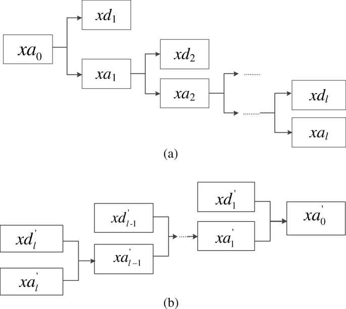

  

  The process of decomposition and reconstruction of the time series by wavelet. a Decomposition process, b Reconstruction process

3.5 Algorithm summary

In this subsection, the proposed PWWTSVR algorithm is illustrated.

The algorithm can be summarized as in Fig. 4.

Fig. 4

Summary of steps performed by PWWTSVR algorithm

4 Experimental results

In this section, some experiments are conducted to examine the performance of PWWTSVR, which is compared to TSVR [4], ε-TSVR [13], TPSVR [15], ν-TWSVR [14], Asy-ν-TSVR [12], KNNUPWTSVR [21], and WL-ε-TSVR [23], using four artificial datasets and eight benchmark datasets. The computer programs for simulation are implemented in a MATLAB R2014a environment on a PC with an Intel Core i5 processor (3.3 Ghz) with 8 GB RAM. In this paper, a Gaussian nonlinear kernel is adopted for all datasets, i.e.,

$$ K(a^{T},b^{T})=exp\left( -\frac{\left\Vert a-b\right\Vert^{2}}{e}\right), \label{kernel} $$

(52)

where a and b are vectors, and e determines the width of the Gaussian function. The choice of parameters is essential for the performance of algorithms. In this paper, parameter values are chosen by the grid-search method from the set of values {10ⁱ|i = − 4,− 3,...,5}. To degrade the computational complexity of parameter selection, let c₁₁ = c₂₁ = c₁, c₁₂ = c₂₂ = c₂, c₁₃ = c₂₃ = c₃ in PWWTSVR; C₁ = C₂ = C, ε₁ = ε₂ = ε in TSVR; c₁ = c₂, c₃ = c₄ in ε-TSVR; c₁ = c₂ = c, ν₁ = ν₂ = ν, λ₁ = λ₂ = λ in TPSVR; c₁ = c₃, c₂ = c₄, ν₁ = ν₂ = ν, in ν −TWSVR; C₁ = C₂ = C, ν₁ = ν₂ = ν in Asy-ν-TSVR; c₁ = c₂, c₃ = c₄, ε₁ = ε₂ = ε in KNNUPWTSVR; and c₁ = c₂ = c, ν₁ = ν₂ = ν, in WL-ε-TSVR.

The performance of PWWTSVR and the other seven methods is evaluated by selected criteria. The number of testing samples is denoted by l, y_i denotes the real value of a testing sample point x_i, $\bar {y}={\sum }_{i} \frac {1}{l}y_{i}$ is the mean value of y₁, y₂,...,y_l, and $\hat {y}_{i}$ denotes the predicted value of x_i. The criteria are specified as follows.

• SSE: Sum squared error of testing samples, defined as SSE=${\sum }_{i = 1}^{m}(y_{i}-\hat {y}_{i})^{2}$.

• SST: Sum squared deviation of testing samples, defined as SST=${\sum }_{i = 1}^{m}(y_{i}-\bar {y}_{i})^{2}$.

• SSR: Sum squared deviation that can be explained by the estimator, defined as SSR=${\sum }_{i = 1}^{m}(\hat {y}_{i}-\bar {y}_{i})^{2}$.

SSE represents the fitting precision. Too small an SSE value may mean overfitting of the regressor due to the fitting of noise. SST represents the variance of the testing samples, and SSR reflects the explanation ability of the regressor.

• SSE/SST: Ratio between sum squared error and sum squared deviation of testing samples, defined as SSE/SST=${\sum }_{i = 1}^{m}(y_{i}-\hat {y}_{i})^{2}/(y_{i}-\bar {y}_{i})^{2}$.

• SSR/SST: Ratio between interpretable sum squared deviation and real sum squared deviation of testing samples, defined as: SSR/SST=${\sum }_{i = 1}^{m}(\hat {y}_{i}-\bar {y}_{i})^{2}/{\sum }_{i = 1}^{m}(y_{i}-\bar {y}_{i})^{2}$.

In most cases, a small SSE/SST represents good agreement between estimates and real values, but too small a value also probably means overfitting of the regressor. SSR/SST shows the variance ratio of the estimated data over the sample data. SSR/SST= 1 means the estimated data have the same variance as training samples.

4.1 Experiments on artificial datasets

To demonstrate the performance of the proposed algorithm on artificial datasets, consider four noised functions for approximation, denoted as y = f(x) + n, where the noise n˜N(0,σ²)is Gaussian additive noise with mean zero and variance σ² being 0.1² and 0.2², respectively. Set the number of training points to 200. Db-3 wavelets used in PWWTSVR are selected to denoise the training data. We compare the performance of seven algorithms (TSVR, ε-TSVR, TPSVR, ν-TWSVR, Asy-ν-TSVR, KNNUPWTSVR, and WL-ε-TSVR) to that of PWWTSVR. Figure 5 shows the one-run approximation functions obtained by PWWTSVR for four artificial functions with different variance noise. The adopted functions for regression are defined in Table 1. The selection of parameters can be seen in Table 2.

Fig. 5

Regression performance of PWWTSVR for noise variance σ² = 0.2² on a Function 1 dataset; b Function 2 dataset; c Function 3 dataset; d Function 4 dataset

Table 1 Function definition and definition domain of artificial datasets

Table 2 Performance and selection of parameters of eight algorithms on artificial datasets with different variance of Gaussian noises

The number of training points and testing points were all set to 200. Testing data were selected randomly under a uniform distribution and assumed to be noise-free. Other settings can be seen in Table 2.

The average results are summarized in Table 2. In the value items, the first item shows the mean value of 10-times testing results and the second represents plus or minus the standard deviation. The values with the lowest SSE, SSE/SST, and CPU time, and the closest SSR/SST to 1 are typeset in bold. Obviously, PWWTSVR obtains the lowest testing errors, and it has the smallest SSE and SSE/SST values among these eight cases. For the value of SSR/SST, PWWTSVR gets a value near to 1 and is close to that of other methods. For calculation time, PWWTSVR gets the smallest value for function 1 and function 2, and the second smallest value for function 3 and function 4. It is slightly higher than that of KNNUPWTSVR, which is also solved in primal space rather than dual space. From the comparisons of the eight algorithms, it can be seen that PWWTSVR has better performance in most criteria.

To further verify the validity of the proposed algorithm, an iterative regression experiment was carried out. The procedure was as follows.

• Step 1: Calculate regression function f(x) using Algorithm 1.

• Step 2: Replace the $\hat {Y}$ in (48) by f(x) and renew the weighting parameter D by (48).

• Step 3: Repeat steps 1 and 2 several times.

Figure 6 shows a one-shot SSE value over iteration times for the regression of function 1. The training number and test number are both set to 500, the variance of noise is 0.2, and other parameters can be seen in Table 2. The STD in Table 3 means the standard deviation of the performance. It shows that the SSE value decreases as the iterations increase, which can verify the effectiveness of adding the weighting parameter D. The quality of pre-regression can determine the regression precision of the proposed method; that is why the iterative process can play a positive role.

Fig. 6

The influence of iterative times on SSE value for Function 1 dataset

Table 3 Comparisons of PWWTSVR on Function 1 with different kernel functions

To test the sensitivity of parameter selection on PWWTSVR regression performance, we studied the influence of parameters c₁, c₂, c₃, E, σ² on SSE, SSE/SST, and SSR/SST for artificial datasets on function 1 and function 2 with noise variance σ² = 0.1². From Fig. 7, we can see that most SSE and SSE/SST curves show convexity, i.e., with the increase of a parameter, the performance value decreases first and then increases, which can ensure that the optimal value can be found. However, their sensitivities to the change of parameter values are different. The performance is sensitive to c₁, c₂, E, σ², but not to c₃.

Fig. 7

Influence of parameter c₁, c₂, c₃, E, σ² on SSE, SSE/SST, and SSR/SST for artificial datasets Function 1 and Function 2 with noise variance σ² = 0.1². The curve of SSE over c₁ for Function 1 is marked as Fun1c1, for example

The selection of a kernel function is important to the performance of regression algorithms. To test the effect of kernel functions, we studied the performance of six kernel functions for artificial datasets on function 1, including the Gaussian kernel adopted in the proposed method. The function expressions and performance are listed in Table 3. It is easy to see that the Gaussian kernel achieves the best results. For linear kernel or polynomial kernel to have high SSE values means that it is not suitable for regression in this kind of problem.

4.2 Experiments on benchmark datasets

To further evaluate the performance of the proposed algorithm, experiments on benchmark datasets from the UCI machine learning repository [29] were conducted. Due to the properties of wavelet transforms, the selected datasets are all time series. Although there are many regression applications of time-series signals, few publicly available datasets are available to use. Information on the selected 14 datasets is summarized in Table 4, including the adopted number of training samples and attributes. Note that the Istanbul stock dataset is used as four datasets by adopting 1/2/4/8 attributes as inputs of algorithms. In addition, one dataset, Concrete, which is not a time series, is used for performance comparison.

Table 4 Benchmark datasets and their number of samples and attributes

• Energy Energy used in a low-energy building.

• Beijing2.5 PM2.5 data of U.S. Embassy in Beijing.

• AirQuality Gas concentrations on the field in an Italian city.

• DowJones Weekly data for the Dow Jones Industrial Index.

• Istanbul Returns of the Istanbul Stock Exchange with seven other international indices.

• PowerConsume Measurements of electric power consumption in one household.

• GHG Emissions of greenhouse gas in California.

• Electricity Electricity consumption of 370 points/ clients.

• DailyDemand Demand data collected from a large Brazilian logistics company.

• SML Indoor environmental data in a house, including temperature, humidity, and carbon dioxide in ppm.

• Concrete Concrete compressive strength, which is a highly nonlinear function of age and ingredients (not a time-series dataset).

For all the real-world examples considered in this paper, the original data are normalized as: $\tilde {s}_{i}=(s_{i}-s_{\min })/(s_{\max }-s_{\min })$, where s_i is the input value of the i th sample, $\tilde {s}_{i}$ is its corresponding normalized value, and s_min and s_max denote the minimum and maximum values, respectively. The parameters are shown in Table 5, which also show the performance of the eight algorithms for the benchmark datasets. The odd-numbered examples are selected as training data, and even-numbered examples as test data, so the amounts of training data and test data are the same. The numbers (m) and dimensions (n) of samples are listed in Table 5. So as not to destroy the character of the time series of the data, one-shot experiments rather than cross-validation experiments are adopted. The values with the lowest SSE, SSE/SST, and CPU time, and the closest SSR/SST to 1 are typeset in bold.

Table 5 Performance and selection of parameters of eight algorithms on benchmark datasets

From Table 5, it can be seen that PWWTSVR outperforms the other algorithms. On most datasets, PWWTSVR obtains the smallest or the second-smallest SSE and SSE/SST value. Only on PowerConsume, GHG, Electricity, and Concrete does PWWTSVR obtain poor values. This is mainly because these datasets have too much noise, or the regularity of change with time is not strong, which will result in weakening or failure of the wavelet-filtering effect. In particular, the contrast dataset Concrete is not a time series, which leads to very poor performance for PWWTSVR. This also illustrates the scope of application of our algorithm. For SSR/SST criteria, PWWTSVR achieves nine of the first or second values which is close to 1 among 14 datasets. It means that the proposed algorithm has nearly the same variance as the original data. From the experimental results of Istanbul1, Istanbul2, Istanbul4, and Istanbul8 (Istanbul datasets with 1/2/4/8 attributes), it can be seen that SSE decreases as the number of input attributes increases, i.e., more input information leads to more accurate estimation. This shows the importance of collecting more information for learning accuracy. For the training time, due to the adoption of the Newton optimization approach in primal space, the PWWTSVR takes the minimum amount of CPU time except for Beijing2.5, Electricity, and DailyDemand. For these datasets, PWWTSVR uses the second shortest CPU time and KNNUPWTSVR the first, and its objective function is also solved in terms of the unconstrained primal problem.

4.3 Statistical analysis

Non-parametric statistical tests were carried out to validate the experimental performance results of the proposed algorithm. The Friedman test [16] was run to rank the algorithms over 22 datasets, including eight artificial datasets and 14 real datasets. The Friedman test had alpha= 0.05 and was distributed according to chi-square with seven degrees of freedom. The Friedman statistic was 43.78, 39.74, and 98.85, with p -values of 2.3595e-7, 1.4112e-6, and 1.8650e-18 for SSE, SSE/SST, and training time, respectively. The average ranks obtained by the eight methods for the criteria SSE, SSE/SST, and training time in the Friedman test are shown in Table 6, from which we can see that the average SSE, SSE/SST, and training time ranks of PWWTSVR are lower than those of other methods. This shows the superiority of the proposed algorithm, which achieves better generalization performance and shorter running times. To check the significant differences between the methods, the p-value was calculated through the Bonferroni-Dunn non-parametric test by computing multiple pairwise comparisons among the proposed algorithm and the other methods. The test assumes that the performances of two algorithms are significantly different if their average ranks differ by at least some critical value [16]. Table 7 lists the p-value of the Bonferroni-Dunn test on the criteria SSE, SSE/SST, and training time ranking results obtained by the Friedman procedure. The null hypothesis of these tests is that there is no difference between the results. From Table 7, we see that the p-value is very small, which means that PWWTSVR is quite different from other methods for SSE, SSE/SST, and training time, and this confirms its superiority.

Table 6 Algorithms’ average rank for SSE, SSE/SST, and CPU time

Table 7 p-value of Bonferroni-Dunn test for SSE, SSE/SST and CPU time comparing our PWWTSVR with other methods

From the above analysis, we can conclude that PWWTSVR can improve the performance of the model and reduce the computation time. The empirical risk term in the objective function is the sum of weighted squared distances from training points to the bound function. Minimizing it causes the function f(x) to fit the training samples and avoiding under-fitting. The regularization term in the objective function is adopted to solve the overfitting problem. The structural risk minimization is implemented by minimizing the regularization term, and solving the problems in the primal space can reduce the computational costs. The introduction of the projection item and weighting parameters into both quadratic and first-degree empirical risk terms are feasible and effective, and the preprocessing of training data by the wavelet transform method can utilize the prior information of samples. It should be noted that wavelet theory is a powerful denoising tool for time-series signals. So, the proposed method is suitable for dealing with time-series datasets. If we deal with non-series samples with the proposed algorithm, performance may suffer. Additionally, the proposed model is suitable for small datasets, and a large number of training samples will incur a tremendous computational cost.

5 Conclusions

In this paper, a projection wavelet weighted twin support vector regression algorithm is proposed. The PWWTSVR calculates the regression function by the mean of up- and down-bound regression functions, which are solved by two small-sized optimization problems in primal space. Unlike the cases in ε-TSVR, each optimization problem of the proposed algorithm aims to seek a suitable projection axis such that the variance of projected points can be minimized. Moreover, samples in different positions in the proposed model are given different weights according to the distance between samples and preprocessed results by wavelet transform. Computational comparisons between PWWTSVR and several existing methods were performed on artificial and benchmark datasets. The experimental results show better generalization performance and demonstrate the effectiveness of the proposed method. The solution of the proposed objective functions based on the Newton iterative approach is deduced in this paper, and the experimental results manifest the advantage in calculation time. However, one can notice that a matrix-inversion process is involved in the algorithm, so it is not suitable for large-scale nonlinear problems. The selection of parameters can obviously affect the performance of PWWTSVR, so for future work, the study of optimal parameter selection and a method involving less calculation could be carried out.

References

Vapnik VN (1995) The natural of statistical learning theroy. Springer, New York
Vapnik VN (1998) Statistical learning theroy. Wiley, New York
Khemchandani JR, Chandra S (2007) Twin support vector machines for pattern classification. IEEE Trans Pattern Anal 29(5):905–910
Peng X (2010) TSVR: an efficient twin support vector machine for regression. Neural Netw 23(3):356–372
Suykens JAK, Lukas L, Dooren V (1999) Least squares support vector machine classifiers: a large scale algorithm. In: Proceedings of ECCTD. Italy, pp 839–842
Suykens JAK, Vandewalle J (1999) Least squares support vector machine classifiers. Neural Process Lett 9(3):293–300
Scholkopf B, Smola AJ, Williamson RC, Bartlett PL (2000) New support vector algorithms. Neurocomputing 12(5):1207–1245
Huang XL, Shi L, Pelckmans K, Suykens JAK (2014) Asymmetric ν-tube support vector regression. Comput Stat Data Anal 77:371–382
Huang XL, Shi L, Suykens JAK (2014) Support vector machine classifier with pinball loss. IEEE Trans Pattern Anal 36:984– 997
Xu Y, Yang Z, Pan X (2016) A novel twin support vector machine with pinball loss. IEEE Trans Neural Netw Learn Syst 28(2):359–370
Xu Y, Yang Z, Zhang Y, Pan X, Wang L (2016) A maximum margin and minimum volume hyper-spheres machine with pinball loss for imbalanced data classification. Knowl-Based Syst 95:75–85
Xu Y, Li X, Pan X, Yang Z (2017) Asymmetric ν-twin support vector regression. Neural Comput Appl 2:1–16
Shao Y, Zhang C, Yang Z, Jing L, Deng N (2013) An ν-twin support vector machine for regression. Neural Comput Appl 23:175–185
Rastogi R, Anand P, Chandra S (2017) A v-twin support vector machine based regression with automatic accuracy control. Appl Intell 46:670–683
Peng X, Xu D, Shen J (2014) A twin projection support vector machine for data regression. Neuro Comput 138:131–141
Melki G, Cano A, Kecman V, Ventura S (2017) Multi-target support vector regression via correlation regressor chains. Info Sci s415–416:53–69
Ding S, Wu F, Shi Z (2014) Wavelet twin support vector machine. Neural Comput Appl 25(6):1241–1247
Melki G, Cano A, Ventura S (2018) MIRSVM: multi-instance support vector machine with bag representatives. Pattern Recogn 79:228–241
Melki G, Kecman V, Ventura S, Cano A (2018) OLLAWV: OnLine learning algorithm using worst-violators. Appl Soft Comput 66:384–393
Xu Y, Wang L (2014) K-nearest neighbor-based weighted twin support vector regression. Appl Intell 41:299–309
Gupta D (2017) Training primal K-nearest neighbor based weighted twin support vector regression via unconstrained convex minimization. Appl Intell 47:962–991
Chapelle O (2007) Training a support vector machine in the primal. Neurocomputing 19(5):1155–1178
Ye Y, Bai L, Hua X, Shao Y, Wang Z, Deng N (2016) Weighted Lagrange ν-twin support vector regression. Neurocomputing 197:53–68
Shevade S, Keerthi S, Bhattacharyya C (2000) Improvements to the SMO algorithm for SVM regression. IEEE Trans Neural Netw 11(5):1188–1193
Lee Y, Hsieh W, Huang C (2005) SSVR: a smooth support vector machine for insensitive regression. IEEE Trans Knowl Data En 17(5):678–685
Peng X, Chen D (2018) PTSVRs: regression models via projection twin support vector machine. Info Sci 435:1–14
Horn RA, Johnson CR (2013) Matrix analysis, 2nd edn. Cambridge University Press, New York
Zhang F (2005) The Schur complement and its applications. Springer, New York
Blake C, Merz C (1998) UCI repository for machine learning databases. http://www.ics.uci.edu/mlearn/MLRepository.html
Acknowledgments
This work was supported by the National Natural Science Foundation of China under Grants 71571091 and 71771112.
Author information
Authors and Affiliations
Corresponding author
Additional information
Publisher’s note
Springer Nature remains neutral with regard to jurisdictional claims in published maps and institutional affiliations.
Rights and permissions
About this article
Cite this article
Wang, L., Gao, C., Zhao, N. et al. A projection wavelet weighted twin support vector regression and its primal solution. Appl Intell 49, 3061–3081 (2019). https://doi.org/10.1007/s10489-019-01422-7
Published:
Issue Date:
DOI: https://doi.org/10.1007/s10489-019-01422-7