Advanced solution framework for time-dependent reliability-based design optimization under fuzzy and interval uncertainties

Abstract

The problem which is actually being addressed in this study includes two parts: One is on establishing time-dependent reliability-based design optimization (tRBDO) formulation under fuzzy and interval uncertainties to obtain the optimal design parameter solution for the time-dependent structure. The other is on presenting a serial single-loop optimization (SSLO) strategy to estimate the optimal design parameter. For addressing the optimal design parameter of the time-dependent structure involving fuzzy and interval uncertainties, a novel tRBDO model with the constraint of time-dependent failure possibility (TDFP) based on the possibility theory of the safety measure is proposed. For evaluating the optimal design parameter, the established SSLO method converts the original triple-loop optimization which is TDFP-index-based approach into a sequence of deterministic optimization, interval value corresponding to the worst case scenario, the estimation of time instant, and the minimum most probable point. Iterative searching step is not needed to find the minimum most probable point at each iteration step in the proposed SSLO strategy; therefore, the computational time is extremely reduced. Several examples are given to demonstrate the efficiency of the proposed approach.

1 Introduction

In most engineering design field, the problem of the game between the low cost and high safety level is widely explored. Traditional deterministic design optimization (DDO), robust design optimization (RDO), and reliability-based design optimization (RBDO) have many achievements in this filed (Schuëller and Jensen 2008). DDO focuses on estimating the optimum solution under the constraint functions without considering uncertainties. However, it is generally known that the uncertainties unavoidably exist in structural geometric dimension, material property, external loading, and other system parameters which are included in the design process (Ling et al. 2019; Hu et al. 2020; Zadeh 1965). These uncertainties may cause structural performance to change or fluctuate, or even cause severe deviation and result in unanticipated or even unprecedented function fault (Yao et al. 2011). Therefore, RDO and RBDO that consider structural uncertainties have been studied in many works, RDO aims at minimizing the variation of the objective function, and RBDO model aims at searching for the optimal solution under reliability constraints considering uncertainties. This paper mainly focuses on RBDO.

As is well known, current research and practice on RBDO are mainly concentrated in probabilistic framework (Keshtegar and Hao 2018; Zhang et al. 2017; Meng and Keshtegar 2019; Royset et al. 2001). Under this framework, calculating the reliability requires precise information of the tail of the random probability distribution (Elishakoff and Ferracuti 2006), and the accurate tail characteristics of the random distribution require large amount of data (Fan et al. 2018). It is too hard for the engineering application to provide so much data for accurately representing the tail distribution, which makes the estimation of the reliability completely unconvincing, and potentially with severe consequences. In allusion to the existing defects represented by probabilistic model in RBDO, interval set and fuzzy sets theory have attracted large attentions in uncertainty representation, and bounds of the uncertainty and the membership function of the fuzzy variables can be generated with few sample data, for example, human behaviors and expert experience (Jiang et al. 2007; Hao et al. 2017; Wang et al. 2019a, 2020, 2019b; Du et al. 2006; Xiong et al. 2019; Wang and Xiong 2019). The practical applications usually face the situation with mixed uncertainties. Some uncertainties involving human behaviors and expert experiences can be measured within a fuzzy set framework, and the bounds of other uncertainties are well-defined, but the sample information is missing and can be represented within an interval variable. Some works focusing on mixed uncertainties have been proposed, such as the mixture of random and interval uncertainties, the combination of random and fuzzy variables, etc.; however, fewer works deal with the time-dependent situation with fuzzy variables and interval variables.

RBDO involving fuzzy uncertainty under different reliability index constraints have been studied (Wang et al. 2019a, 2017; Tang et al. 2014; Du et al. 2006; Du and Choi 2008; Mourelatos and Zhou 2005). Wang et al. proposed a sequential optimization and fuzzy reliability analysis method for multidisciplinary systems to decouple the fuzzy reliability analysis from the optimization; furthermore, a novel adaptive collocation method is established to analyze the fuzzy reliability for multidisciplinary systems (Wang et al. 2019a). A new formulation of possibility-based design optimization using the performance measure approach (PMA) is established by Du and Choi; for the inverse possibility analysis, the maximal possibility search method is proposed to improve numerical efficiency and accuracy (Du et al. 2006). Wang et al. proposed a credibility-based design optimization, and the sequential optimization and credibility assessment are established to solve the credibility-based design optimization (Wang et al. 2020). Tang et al. presented the possibilistic safety index-based design optimization model for structures with fuzzy variable vector, and a technique called target performance-based design approach is proposed to solve the optimization model (Tang et al. 2014). A hybrid reliability-based optimization model is established with random, interval, and fuzzy parameters, and a subinterval vertex method is presented to calculate the optimization model (Wang et al. 2017). A possibility-based design optimization method is proposed, and a computationally efficient and accurate hybrid (global–local) optimization approach is subsequently described for calculating the confidence level of fuzzy response, the method combines the advantages of the commonly used vertex and discretization methods (Mourelatos and Zhou 2005). By approximating the fuzzy credibility constraint by the adaptive kriging surrogate model, a fuzzy credibility-based design is decoupled to a common deterministic optimization (Jia et al. 2020).

All RBDO involving the fuzzy uncertainty in the literature mentioned above deal with the time-independent structure. The time-dependent reliability-based design optimization (tRBDO) under the mixed fuzzy uncertainty and interval uncertainties is seldom investigated in the reported literatures. Therefore, this work firstly constructs a tRBDO with time-dependent failure possibility (TDFP) constraints involving fuzzy and interval variables. The TDFP can measure the safety degree of the time-dependent structure (Fan et al. 2019). The TDFP-index-based approach is investigated to solve the tRBDO, but the computational cost is extremely high for engineering application. In order to improve the efficiency of the solution of tRBDO, (extreme value combined performance measure approach) EVCPMA is proposed which is motivated by the performance measure approach (Tu et al. 1999) and concerned performance-based approach (Kang et al. 2011). The TDFP-index-based approach and EVCPMA is a double-loop optimization strategy, in which the outer loop is a deterministic optimization, and the inner loop is reliability analysis. Meanwhile, the TDFP analysis is a double-loop optimization for the structure involving fuzzy and interval uncertainties; therefore, the computation burden of the tRBDO of the engineering problem is unbearable. To decrease the high computational cost, a serial single-loop optimization (SSLO) is established in this work to deal with the tRBDO with fuzzy and interval uncertainties. Generally, directly solving this problem needs a triple-loop optimization process in which the outer loop solves the optimal parameters, the middle loop computes the minimum performance of constraint function with respect to the interval variables, and the inner loop evaluates the TDFP. In the proposed SSLO, the original triple-loop optimization is converted into a sequence of deterministic optimization, the evaluation of time instant and interval value correspond to the worst case scenario, and the minimum most probable point searching. Thus, the efficiency of the solution of the tRBDO model is greatly improved by the SSLO method. It should be noted that the main aim of this work is to propose a new estimation strategy for solving the tRBDO involving fuzzy and interval uncertainties. The SSLO is proposed by extending the idea in Ref. (Du and Chen 2004) and integrating with the definition of the TDFP. Original sequential optimization and reliability assessment is employed to solve RBDO involving random variable.

This paper is organized as follows. In Sect. 2, the TDFP safety model of structure with fuzzy and interval variable vector is reviewed. The tRBDO involving fuzzy and interval uncertainties is proposed, and the double-loop optimization strategy is established which is TDFP-index-based approach and EVCPMA in Sect. 3. Section 4 provides SSLO method to calculate the optimal solutions. Six applications are given to demonstrate the rationality and computational efficiency of the proposed approach in Sect. 5. A summary and conclusions are given in Sect. 6.

2 Formulation of tRBDO under fuzzy and interval uncertainties

For the time-dependent structure with fuzzy and interval uncertainties, its performance function can be expressed as $g({\mathbf{Z}},{\mathbf{Y}},t)$, where ${\mathbf{Z}}$ is the $n_{Z} -$ dimensional fuzzy input variable vector which is characterized by the membership function $u_{{\mathbf{Z}}}$, ${\mathbf{Y}} \in [{\mathbf{\underline {Y} }},{\overline{\mathbf{Y}}}]$ is the $n_{Y} -$ dimensional interval input variable vector with upper boundary ${\overline{\mathbf{Y}}}$ and lower boundary ${\mathbf{\underline {Y} }}$, $t \in [t_{0} ,t_{e} ]$ is the time parameter. Generally, the failure state corresponds to negative values of $g({\mathbf{Z}},{\mathbf{Y}},t)$, and the safe state corresponds to positive values of $g({\mathbf{Z}},{\mathbf{Y}},t)$. According to the propagation theory of the interval uncertainty, the time-dependent failure possibility (TDFP) is an interval variable because of the interval input variables ${\mathbf{Y}}$. The TDFP is denoted as $\pi_{ft} ({\mathbf{Y}})$, and the mathematical expression of $\pi_{ft} ({\mathbf{Y}})$ is defined as

$$\begin{aligned} \pi_{ft} ({\mathbf{Y}}) & = {\text{poss}}\{ g({\mathbf{Z}},{\mathbf{Y}},t) \le 0,\exists t \in [t_{0} ,t_{e} ]\} \\& = \sup \{ \alpha |g({\mathbf{Z}},{\mathbf{Y}},t) \le 0,\exists t \in [t_{0} ,t_{e} ]\} , \\ \end{aligned}$$

(1)

where ${\text{poss}}\{ \cdot \}$ and $\sup ( \cdot )$ represent the possibility operator and supremum operator, $\exists t \in [t_{0} ,t_{e} ]$ means there is a time node $t$ in $[t_{0} ,t_{e} ]$, $\alpha \in [0,1]$ is the membership level of the output response.

From Eq. (1), one can see that the TDFP model can measure the safety degree of structure under the fuzzy and interval uncertainties over a specified time interval. The TDFP is defined as the possibility of the performance less than zero under the fuzzy and interval uncertainties at a given time interval $t \in [t_{0} ,t_{e} ]$. The expression $\mathop {\min }\limits_{{t \in [t_{0} ,t_{e} ]}} g({\mathbf{Z}},{\mathbf{Y}},t)$ which is independent of the time parameter $t$ is extreme value response of $g({\mathbf{Z}},{\mathbf{Y}},t)$, thus following $\mathop {\min }\limits_{{t \in [t_{0} ,t_{e} ]}} g({\mathbf{Z}},{\mathbf{Y}},t)$ can be denoted as $g_{\min } ({\mathbf{Z}},{\mathbf{Y}})$. By the extreme value transformation of the time-dependent performance function, the TDFP is equivalent to the time-independent failure possibility of the extreme value response $g_{\min } ({\mathbf{Z}},{\mathbf{Y}})$ of $g({\mathbf{Z}},{\mathbf{Y}},t)$ as follows:

$$\pi _{{ft}} ({\mathbf{Y}}) = {\text{Poss}}\{ g_{{\min }} ({\mathbf{Z}},{\mathbf{Y}}) \le 0\} = \sup \{ \alpha |g_{{\min }} ({\mathbf{Z}},{\mathbf{Y}}) \le 0\} .$$

(2)

According to the formulation of the TDFP, two basic properties can be concluded. Firstly, the value of the TDFP is bounded in interval $[0,1]$. Secondly, if the start of the time $t_{0}$ and the interval variable ${\mathbf{Y}}$ are fixed, $\pi_{ft}$ is non-decreasing function of the upper boundary $t_{e}$.

The TDFP $\pi_{ft} ({\mathbf{Y}})$ is an interval variable, and the upper boundary $\overline{\pi }_{ft} ({\mathbf{Y}})$ and lower boundary $\underline {\pi }_{ft} ({\mathbf{Y}})$ of the TDFP $\pi_{ft} ({\mathbf{Y}})$ can be, respectively, computed by

$$\overline{\pi }_{ft} ({\mathbf{Y}}) = \mathop {\max }\limits_{{{\mathbf{Y}} \in [{\mathbf{\underline {Y} }},{\overline{\mathbf{Y}}}]}} \pi_{ft} ({\mathbf{Y}}),$$

(3)

$$\underline {\pi }_{ft} ({\mathbf{Y}}) = \mathop {\min }\limits_{{{\mathbf{Y}} \in [{\mathbf{\underline {Y} }},{\overline{\mathbf{Y}}}]}} \pi_{ft} ({\mathbf{Y}}).$$

(4)

Generally, the upper boundary $\overline{\pi }_{ft} ({\mathbf{Y}})$ of the TDFP $\pi_{ft} ({\mathbf{Y}})$ demonstrates the worst case scenario of the structure. Consequently, the upper boundary $\overline{\pi }_{ft} ({\mathbf{Y}})$ of the TDFP is used to measure the reliability in constraints for establishing the tRBDO model under fuzzy and interval uncertainties. Denote the interval variable value corresponding to the upper boundary $\overline{\pi }_{ft} ({\mathbf{Y}})$ of the TDFP of the $i{\text{th}}$ possibility constraint as ${\mathbf{Y}}_{i}^{ * }$; therefore, the tRBDO model under fuzzy and interval uncertainties can be defined as follows:

$$\begin{array}{*{20}l} {\min } & {f({\mathbf{d}},{\mathbf{X}}^{c} )} \\ {{\text{s}}{\text{.t}}{.}} & {{\text{poss}}\{ g_{i} ({\mathbf{d}},{\mathbf{Z}},{\mathbf{Y}}_{i}^{ * } ,t) \le 0,\exists t \in [t_{0} ,t_{e} ]\} \le \pi_{fti}^{ * } {\kern 1pt} (i = 1,2, \ldots ,n_{g} )} \\ {} & {{\mathbf{Z}} = [{\mathbf{X}},{\mathbf{P}}],{\mathbf{Y}}_{i}^{ * } \in [{\mathbf{\underline {Y} }},{\overline{\mathbf{Y}}}],{\mathbf{d}}^{L} \le {\mathbf{d}} \le {\mathbf{d}}^{U} ,{\mathbf{X}}^{L} \le {\mathbf{X}}^{c} \le {\mathbf{X}}^{U} } \\ \end{array}$$

(5)

where

$${\mathbf{Y}}_{i}^{ * } = \arg \mathop {\max }\limits_{{{\mathbf{Y}} \in [{\mathbf{\underline {Y} }},{\overline{\mathbf{Y}}}]}} \pi_{fti} ({\mathbf{Y}}),$$

(6)

$f({\mathbf{d}},{\mathbf{X}}^{c} )$ denotes the objective function, which is generally the commercial cost or the weight of structure in engineering design. $g_{i} ({\mathbf{d}},{\mathbf{Z}},{\mathbf{Y}}_{i}^{ * } ,t)$ ${\kern 1pt} (i = 1,2, \ldots ,n_{g} )$ is the performance function of the $i{\text{th}}$ TDFP constraint. ${\mathbf{d}}$ means the $n_{d}$-dimensional deterministic design parameter vector with the upper boundary and lower boundary are ${\mathbf{d}}^{U}$ and ${\mathbf{d}}^{L}$ , respectively. ${\mathbf{X}}$ represents the $n_{X}$-dimensional fuzzy design vector with nominal value vector ${\mathbf{X}}^{c}$, and the upper and lower boundary of ${\mathbf{X}}^{c}$ are ${\mathbf{X}}^{U}$ and ${\mathbf{X}}^{L}$ , respectively. ${\mathbf{P}}$ is the $n_{P}$-dimensional fuzzy parameter vector and $\pi_{fti}^{ * } {\kern 1pt}$ represents the target TDFP index of the $i{\text{th}}$ reliability constraint. It should be noted that ${\mathbf{Y}}_{i}^{ * }$ is generally unknown before estimating the TDFP $\pi_{fti} ({\mathbf{Y}})$ for different design parameter solutions. It is a nested process for calculating ${\mathbf{Y}}_{i}^{ * }$ in solving tRBDO with fuzzy and interval uncertainties. In this work, a sequential single-loop process is established to efficiently estimate ${\mathbf{Y}}_{i}^{ * }$ and solve the tRBDO model shown in Eq. (3).

3 Solution strategy of the tRBDO with fuzzy and interval uncertainty

In this section, we introduce two basic strategies with the double-loop method, which is preparatory work for our proposed method. Results from these two strategies are compared with those from our established method in final applications.

3.1 TDFP-index-based approach

The typical solution of tRBDO is a double-loop nested optimization, the outer loop is a deterministic optimization process, and the inner loop is the TDFP analysis process. The detailed implementation of the double-loop optimization method (DLOM) to estimated TDFP can refer to the literature (Fan et al. 2019). The TDFP-index-based approach cannot be directly applied to the formulation of Eq. (5), thus the original tRBDO formulation involving fuzzy and interval uncertainties can be expressed as follows:

$$\begin{array}{*{20}l} {\min } & {f({\mathbf{d}},{\mathbf{X}}^{c} )} \\ {{\text{s}}{\text{.t}}{.}} & {{\text{poss}}\{ g_{i} ({\mathbf{d}},{\mathbf{Z}},{\mathbf{Y}},t) \le 0,\exists t \in [t_{0} ,t_{e} ]\} \le \pi_{fti}^{ * } (i = 1,2, \ldots ,n_{g} )} \\ {} & {{\mathbf{Z}} = [{\mathbf{X}},{\mathbf{P}}],{\mathbf{Y}} \in [{\mathbf{\underline {Y} }},{\overline{\mathbf{Y}}}],{\mathbf{d}}^{L} \le {\mathbf{d}} \le {\mathbf{d}}^{U} ,{\mathbf{X}}^{L} \le {\mathbf{X}}^{c} \le {\mathbf{X}}^{U} } \\ \end{array} .$$

(7)

The TDFP-index-based approach is not the focus of this article; thus, the basic solution idea of the TDFP-index-based approach is described in the following. Based on the Eq. (1), the initialization of the design variable ${\mathbf{d}}^{(0)}$ and ${\mathbf{X}}^{{C^{0} }}$ is set in the outer loop which is the deterministic optimization process. Secondly, the TDFP analysis in the inner loop is given in the following. In the DLOM, the time interval $[t_{0} ,t_{e} ]$ and the interval variables ${\mathbf{Y}}$ are discretized, and then time-independent failure possibility (TIFP) for every discrete time instant and a discrete point of interval variables ${\mathbf{Y}}$ is computed; the computation of TIFP is divided into two steps: one step is that the membership function of the performance is estimated by discretizing the membership level (Graf et al. 2000), and another is that the TIFP is addressed with the simple interpolation. Thereupon, the TDFP for a discrete point of interval variables is the maximum of the values of the TIFP for all discretized time instants. Finally, $\overline{\pi }_{ft} ({\mathbf{Y}})$ is the maximum of the values of the $\pi_{ft}$ for all discretized points of the interval variables. According to Eq. (7), the optimal design parameter should fulfill inequality $\overline{\pi }_{fti} ({\mathbf{Y}}) \le \pi_{fti}^{ * } {\kern 1pt}$$i = 1,2, \ldots ,n_{g}$. When the numbers of discretized time parameter $t$ and interval variables ${\mathbf{Y}}$ are extremely huge, the $\overline{\pi }_{ft} ({\mathbf{Y}})$ will converge. Thus, the TDFP-index-based approach with DLOM is time-consuming for engineering problem.

The solution of the TDFP-index-based approach with single-loop optimization method (SLOM) in the outer loop is a deterministic optimization process that is same with the TDFP-index-based approach with DLOM. From Eq. (2), the solution of TDFP analysis with SLOM in the inner loop is introduced as follows: The SLOM only discretizes the membership level $\alpha \in [0,1]$ and estimates the lower boundary of the minimum $g_{\min }^{(L)} ({\mathbf{d}},{\mathbf{Z}},{\mathbf{Y}})$ for each discrete membership level by Eq. (8). Finally, $\overline{\pi }_{fti} ({\mathbf{Y}})$ is addressed with the simple interpolation. From Eq. (7), the optimal design parameter should fulfill inequality $\overline{\pi }_{fti} ({\mathbf{Y}}) \le \pi_{fti}^{ * } {\kern 1pt}$$i = 1,2, \ldots ,n_{g}$. Thus, the SLOM is more efficient than the DLOM to estimate the tRBDO with fuzzy and interval uncertainties.

$$\begin{array}{*{20}l} {\min } & {g({\mathbf{d}}^{{(k)}} ,{\mathbf{Z}}^{{(k)}} ,{\mathbf{Y}},t)} \\ {{\text{s}}{\text{.t}}.} & {{\mathbf{Z}}^{{(k)}} (\alpha _{i} ) \in [{\mathbf{Z}}^{{(k)(L)}} (\alpha _{i} ),{\mathbf{Z}}^{{(k)(U)}} (\alpha _{i} )](i = 1,2, \ldots ,m)} \\ {} & {{\mathbf{Y}} \in [{\mathbf{\underset{\raise0.3em\hbox{$\smash{\scriptscriptstyle-}$}}{Y} }},\overline{{\mathbf{Y}}} ]} \\ {} & {t \in [t_{0} ,t_{e} ]} \\ \end{array}$$

(8)

where ${\mathbf{d}}^{(k)}$ and ${\mathbf{Z}}^{(k)}$ are the realization in the $k{\text{th}}$ iteration, $m$ is the discretized number of the membership level $\alpha$.

3.2 Extreme value combined performance measure approach

The performance measure approach (PMA) is widely used in RBDO involving random uncertainty (Huang et al. 2016; Zhang et al. 2017), and PMA is introduced to analyze the RBDO with fuzzy uncertainty with inverse possibility analysis method (Du et al. 2006). Actually, the PMA can be achieved by the following equivalent constraint transformation:

$${\text{Poss}} \{ G_{\min } ({\mathbf{d}},{\mathbf{Z}},{\mathbf{Y}}_{i}^{ * } ) \le 0\} - \pi_{fti}^{ * } \le 0 \Leftrightarrow G_{\min }^{(L)} ({\mathbf{d}},{\mathbf{Z}}(\pi_{fti}^{ * } ),{\mathbf{Y}}_{i}^{ * } ) \ge 0$$

(9)

Based on the equivalent constrain transformation by Eq. (9), the tRBDO formulation defined by Eq. (7) can be transformed as follows:

$$\begin{array}{*{20}l} {\mathop {\min }\limits_{{\mathbf{d}}} } & {f({\mathbf{d}},{\mathbf{X}}^{c} )} \\ {{\text{s}}{\text{.t}}.} & {g_{{i\min ^{{(L)}} }} ({\mathbf{d}},{\mathbf{Z}}(\pi _{{fti}}^{*} ),{\mathbf{Y}}_{i}^{*} ) \ge 0} \\ {} & {{\mathbf{d}}^{L} \le {\mathbf{d}} \le {\mathbf{d}}^{U} } \\ {} & {{\mathbf{X}}^{L} \le {\mathbf{X}}^{c} \le {\mathbf{X}}^{U} } \\ {} & {0 \le \pi _{{fti}}^{*} \le 1} \\ {} & {i = 1,2, \ldots ,{\text{N}}_{c} } \\ \end{array}.$$

(10)

where $g_{{i\min }}^{{(L)}} ({\mathbf{d}},{\mathbf{Z}}(\pi _{{fti}}^{ * } ),{\mathbf{Y}})$ can be estimated with Eq. (8) at the target membership level $\pi_{fti}^{ * }$.

From Eq. (10), the conclusion can be easily deduced that extreme value combined performance measure approach is more efficient than the TDFP-index-based method, since the target performance is considered at the target membership level $\pi_{fti}^{ * }$.

4 Serial single-loop optimization strategy

In this section, maximal possibility search approach is firstly introduced, and then the detailed SSLO strategy is established.

4.1 Most probable point searching

In this study, it is assumed that the membership function of the independent input fuzzy variable vector ${\mathbf{Z}}$ satisfies three properties (Dubois and Prade 1987; Cremona and Gao 1997): (1) unity, (2) strong convexity, and (3) bounded. These three properties can guarantee the independent input fuzzy variable vector be uniquely transformed to the standard normalized fuzzy variable vector ${\mathbf{V}}$, For instance, the Gaussian membership function is formulated as

$$u_{{Z_{i} }} (z_{i} ) = \exp \left[ { - \left( {\frac{{Z_{i} - Z_{i}^{c} }}{{\sigma_{{Z_{i} }} }}} \right)} \right]^{2} ,\quad i = n_{Z} = n_{X} + n_{P} .$$

(11)

The transformation can be written as

$$V_{i} = \frac{{Z_{i} - Z_{i}^{c} }}{{\sigma_{{Z_{i} }} }},$$

(12)

where $Z_{i}^{c}$ is fuzzy mean of $Z_{i}$, $\sigma_{{Z_{i} }}$ represents fuzzy standard variance, and the membership function of $V_{i}$ is $\exp [ - (V_{i} )^{2} ]$.

The inverse most probable point problem is formulated and shown in the following minimization model(Du et al. 2006),

$$\begin{array}{*{20}l} {{\text{find}}} & {{\text{MPP}}_{{V_{{\pi_{fti}^{ * } }}^{ * } }} } \\ {\min } & {g_{i} ({\mathbf{d}},{\mathbf{V}},{\mathbf{Y}}_{i}^{ * } ,t)} \\ {{\text{s}}{\text{.t}}{.}} & {\left\| {\mathbf{V}} \right\|_{\infty } \le 1 - \pi_{fti}^{ * } } \\ \end{array} ,$$

(13)

where ${\mathbf{V}} = ({\mathbf{V}}_{{\mathbf{X}}} ,{\mathbf{V}}_{{\mathbf{P}}} )$, ${\text{MPP}}_{{V_{{\pi_{fti}^{ * } }}^{ * } }}$ is the optimum point on the target possibility domain $\;\left\| {\mathbf{V}} \right\|_{\infty } \le 1 - \pi_{fti}^{ * }$ is identified as the most probable point with the prescribed possibility of TDFP $\pi_{fti}^{ * }$. $\;\left\| {\mathbf{V}} \right\|_{\infty }$ is the Infinite norm of the vector ${\mathbf{V}}$.

By the inverse most probable point search algorithm, the optimum solution of most probable point ${\text{MPP}}_{{V_{{\pi_{fti}^{ * } }}^{ * } }}$ can be identified and extreme value combined performance measure approach is evaluated by

$$\begin{aligned} g_{i\min }^{(L)} ({\mathbf{d}},{\mathbf{Z}}(\pi_{fti}^{ * } ),{\mathbf{Y}}_{i}^{ * } )& = {\text{g}}_{i\min } {(}{\mathbf{d}}{\text{,MPP}}_{{V_{{\pi_{fti}^{ * } }}^{ * } }} ,{\mathbf{Y}}_{i}^{ * } {)} \\ & = {\text{g}}_{i\min } ({\mathbf{d}},{\text{MPP}}_{{X_{{\pi_{fti}^{ * } }}^{ * } }} ,{\text{MPP}}_{{P_{{\pi_{fti}^{ * } }}^{ * } }} ,{\mathbf{Y}}_{i}^{ * } ). \\ \end{aligned}$$

(14)

The solution of ${\text{MPP}}_{{V_{{\pi_{fti}^{ * } }}^{ * } }}$ in the literature (Du et al. 2006) is dealt with maximal possibility search method. In this article, the single-loop optimization is proposed for inverse most probable point analysis to ensure numerical efficiency and accuracy in tRBDO under fuzzy and interval uncertainties. The detailed analysis process is given in next subsection.

4.2 The solution of the tRBDO with SSLO strategy

To improve the efficiency of tRBDO analysis, we adopt in this work the strategy of a sequential optimization and TDFP assessment to develop SSLO method. The SSLO method is different from the TDFP-index-based approach and extreme value combined performance measure approach in the way that equivalent deterministic constraints from the TDFP constraints are established. We also employ an efficient inverse most probable point search algorithm as an integral part of the proposed procedure.

To this end, we use the extreme value combined performance measure approach for TDFP constraints with the SSLO method. Based on Eq. (14), the design model (10) is rewritten as

$$\begin{array}{*{20}l} {\mathop {\min }\limits_{{\mathbf{d}}} } & {f({\mathbf{d}},{\mathbf{X}}^{c} )} \\ {{\text{s}}{\text{.t}}{.}} & {{\text{g}}_{i\min } ({\mathbf{d}},{\text{MPP}}_{{X_{{\pi_{fti}^{ * } }}^{ * } }} ,{\text{MPP}}_{{P_{{\pi_{fti}^{ * } }}^{ * } }} ,{\mathbf{Y}}_{i}^{ * } ) \ge 0} \\ {} & {{\mathbf{d}}^{L} \le {\mathbf{d}} \le {\mathbf{d}}^{U} } \\ {} & {{\mathbf{X}}^{L} \le {\mathbf{X}}^{c} \le {\mathbf{X}}^{U} } \\ {} & {0 \le \pi_{fti}^{ * } \le 1} \\ {} & {i = 1,2, \ldots ,{\text{N}}_{c} } \\ \end{array} .$$

(15)

This model establishes the equivalence between a possibility optimization and a deterministic optimization since the original constraint function ${\text{g}}_{{i\min }} ({\mathbf{d}},{\text{MPP}}_{{X_{{\pi _{{fti}}^{*} }}^{*} }} ,{\text{MPP}}_{{P_{{\pi _{{fti}}^{*} }}^{*} }} ,{\mathbf{Y}}_{i}^{*} )$ is used to evaluate design feasibility using the inverse most probable point corresponding to the extreme value combined performance measure approach. It is noted that in a possibility design, most of the computations are used for TDFP assessments. Therefore, to improve the efficiency of possibility optimization, we need to reduce the number of reliability estimation as much as possible. The essence is to move the design solution as quickly as possible to its optimum to reduce the most probable point searching.

The realization process diagram is shown in Fig. 1. In this illustrative diagram, only two fuzzy design variables $X_{1}$ and $X_{2}$ are considered, there are no fuzzy parameters ${\mathbf{P}}$. For the constraint $g_{{i\min }} (X_{1}^{c} ,X_{2}^{c} ,Y_{i}^{*} ) = 0$ (Fig. 1), the actual TDFP (possibility of constraint being feasible) is only around 0.5. After the deterministic optimization, the TDFP assessment is implemented at the optimum solution ${\mathbf{X}} = (X_{1}^{c} ,X_{2}^{c} )$ to locate the inverse ${\text{MPP}}_{{X_{{\pi_{fti}^{ * } }}^{ * } }}$ corresponding to the target safety level. ${\text{MPP}}_{{X_{{\pi_{fti}^{ * } }}^{ * } }}$ of constraint $g_{{i\min }} (X_{1}^{c} ,X_{2}^{c} ,Y_{i}^{ * } )$ falls outside (to the left) the deterministic feasible region, but the ${\text{MPP}}_{{X_{{\pi_{fti}^{ * } }}^{ * } }}$ that corresponds to the target safety level should fall within the deterministic feasible region to ensure the feasibility of a TDFP constraint. Therefore, when establishing the equivalent deterministic optimization model in next cycle, the constraints should be updated to shift ${\text{MPP}}_{{X_{{\pi_{fti}^{ * } }}^{ * } }}$ onto the deterministic boundary to insure the feasibility of the possibility constraint. The formulation of this realization process which is mentioned as SSLO is proved in the following subsection.

Fig. 1

Shift constraint boundary

From Fig. 1, we employ the following equivalent deterministic optimization based on SSOL to solve Eq. (15), in which extreme value and ${\mathbf{Y}}_{i}^{ * }$ are iteratively updated.

$$\begin{array}{*{20}l} {\mathop {\min }\limits_{{\mathbf{d}}} } & {f({\mathbf{d}},{\mathbf{X}}^{c} )} \\ {{\text{s}}{\text{.t}}.} & {g_{{i\min }} ({\mathbf{d}},{\mathbf{X}}^{c} - {\mathbf{S}}_{i}^{{(k)}} ,{\text{MPP}}_{{P_{{\pi _{{fti}}^{*} }}^{*} }}^{{(k)}} ,{\mathbf{Y}}_{i}^{{*(k)}} ) \ge 0} \\ {} & {{\mathbf{d}}^{L} \le {\mathbf{d}} \le {\mathbf{d}}^{U} } \\ {} & {{\mathbf{X}}^{L} \le {\mathbf{X}}^{c} \le {\mathbf{X}}^{U} } \\ {} & {0 \le \pi _{{fti}}^{*} \le 1} \\ {} & {i = 1,2, \ldots ,{\text{N}}_{c} } \\ \end{array},$$

(16)

in which ${\mathbf{S}}_{i}^{(k)}$ is the shifting vector in the $k{\text{th}}$ iteration and it is estimated by

$${\mathbf{S}}_{i}^{{(k)}} = {\mathbf{X}}^{{c(k - 1)}} - {\text{MPP}}_{{X_{{\pi _{{fti}}^{*} }}^{*} }}^{{(k - 1)}}$$

(17)

where $X^{{c(k - 1)}}$ and ${\text{MPP}}^{(k - 1)}_{{X_{{\pi_{fti}^{ * } }}^{ * } }}$ are the nominal value vector and most probable point in the $(k - 1){\text{th}}$ iteration in the original possibility space. ${\text{MPP}}^{(k - 1)}_{{X_{{\pi_{fti}^{ * } }}^{ * } }}$ can be converted into the ${\text{MPP}}_{{V_{X}^{*} \pi _{{fti}}^{*} }}^{{(k - 1)}}$ in the standard normal space based on Eq. (12) with the Gaussian fuzzy distribution.

Directly solving ${\text{MPP}}_{{V_{{\pi_{fti}^{ * } }}^{ * } }}$ needs a nested triple-loop optimization, in which the outer loop addresses the upper boundary of the TDFP with respect to interval variable ${\mathbf{Y}}$ as follows:

$$\left\{ {\begin{array}{*{20}l} {{\text{find}}} & {{\mathbf{Y}}_{i}^{{ * (k)}} } \\ {\min } & {g_{{i\min }} ({\mathbf{d}}^{{(k - 1)}} {\text{,MPP}}^{{(k - 1)}} _{{V_{{\pi _{{fti}}^{ * } }}^{ * } }} ,{\mathbf{Y}})} \\ {\text{s.t.}} & {{\mathbf{Y}} \in [{\mathbf{\underset{\raise0.3em\hbox{$\smash{\scriptscriptstyle-}$}}{Y} }},{\mathbf{\bar{Y}}}]} \\ \end{array} } \right.$$

(18)

The middle loop estimates the extreme value of possibility constraint function with respect to time parameter $t$ which is formulated as

$$\left\{ {\begin{array}{*{20}l} {{\text{find}}} & {t_{i}^{{ * (k)}} } \\ {\min } & {g_{i} ({\mathbf{d}}^{{(k - 1)}} {\text{,MPP}}^{{(k - 1)}} _{{V_{{\pi _{{fti}}^{ * } }}^{ * } }} ,{\mathbf{Y}}_{i}^{{(k)}} ,t)} \\ {{\text{s}}{\text{.t}}{\text{.}}} & {t \in [t_{0} ,t_{e} ]} \\ \end{array} } \right.$$

(19)

The inner loop calculates the most probable point by

$$\left\{ {\begin{array}{*{20}l} {{\text{find}}} & {{\text{MPP}}^{{(k - 1)}} _{{V_{{\pi _{{fti}}^{ * } }}^{ * } }} } \\ {\min } & {g_{i} ({\mathbf{d}}^{{(k - 1)}} ,{\mathbf{V}},{\mathbf{Y}}_{i}^{{ * (k)}} ,t_{i}^{{ * (k)}} )} \\ {{\text{s}}{\text{.t}}{\text{.}}} & {\left\| {\mathbf{V}} \right\|_{\infty } \le 1 - \pi _{{fti}}^{ * } } \\ \end{array} } \right.$$

(20)

where ${\mathbf{d}}^{(k - 1)}$ is the deterministic design parameter vector solution in the $(k - 1){\text{th}}$ iteration.

Calculating this nested triple-loop optimization will cause extremely computational demand. We propose to estimate this nested triple-loop optimization by the single-loop optimization process with Eq. (21).

$$\left\{ {\begin{array}{*{20}l} {{\text{find}}} & {{\mathbf{Y}}_{i}^{{*(k)}} ,t_{i}^{{*(k)}} ,{\text{MPP}}_{{V_{{\pi _{{fti}}^{*} }}^{*} }}^{{(k)}} } \\ {\min } & {g_{i} ({\mathbf{d}}^{{(k - 1)}} ,{\mathbf{V}}(\pi _{{fti}}^{*} ),{\mathbf{Y}},t)} \\ {{\text{s}}{\text{.t}}.} & {t \in [t_{0} ,t_{e} ]} \\ {} & {{\mathbf{Y}} \in [{\mathbf{\underset{\raise0.3em\hbox{$\smash{\scriptscriptstyle-}$}}{Y} }},\overline{{\mathbf{Y}}} ]} \\ {} & {V \in [V^{{(L)}} (\pi _{{fti}}^{*} ),V^{{(U)}} (\pi _{{fti}}^{*} )]} \\ \end{array} } \right.$$

(21)

It is easy to find that the formulation shown in Eq. (21) for searching most probable point under the mixture of fuzzy variable vector, interval variable vector and time parameter are similar to the general situation where only fuzzy variable vector under the same input dimensional condition at target TDFP is $\pi_{fti}^{ * }$ being contained. Therefore, the computational demand of this proposed single-loop optimization is generally in the same order of magnitude as most probable point searching with only fuzzy variable vector.

Above analysis shows that the proposed SSLO strategy addresses the tRBDO by a sequence of deterministic optimization and shifting vector estimation, in which the shifting vector is estimated by the proposed single-loop optimization. Consequently, the proposed SSLO is an accurate and efficient method to solve the tRBDO formulation.

4.3 Implementation of SSLO strategy

The estimation procedure of the proposed SSLO is briefly summarized in this section. The most probable point searching in SSLO as well as the deterministic optimization is solved by the FMINCON toolbox in MATLAB. The convergence criterion is set to be the relative errors of two adjacent objective performances and do not exceed $\varepsilon { = }10^{ - 3}.$

• Step 1 Set the initial design parameter solution ${\mathbf{d}}^{(0)}$, ${\mathbf{X}}^{{c(0)}}$, the most probable point ${\text{MPP}}_{{V_{{\pi_{fti}^{ * } }}^{ * } }}^{(0)}$, the time instant $t_{i}^{{*(0)}}$ and estimate the corresponding objective performance $f^{{(0)}} ({\mathbf{d}}^{{(0)}} ,{\mathbf{X}}^{{c(0)}} )$ and let $k = 1$.

• Step 2 Employ the single-loop optimization shown in Eq. (21) in Fig. 2 to address the updated time instant $t_{i}^{{*(k)}}$, ${\mathbf{Y}}_{i}^{{*(k)}}$ , and ${\text{MPP}}^{(k)}_{{V_{{\pi_{fti}^{ * } }}^{ * } }}$. Convert ${\text{MPP}}^{(k)}_{{V_{{\pi_{fti}^{ * } }}^{ * } }}$ to the original possibility space ${\text{MPP}}^{(k)}_{{Z_{{\pi_{fti}^{ * } }}^{ * } }}$ by Eq. (12) involving Gaussian fuzzy distribution. Calculate the shifting vector ${\mathbf{S}}_{i}^{(k)}$ by Eq. (17).

  Fig. 2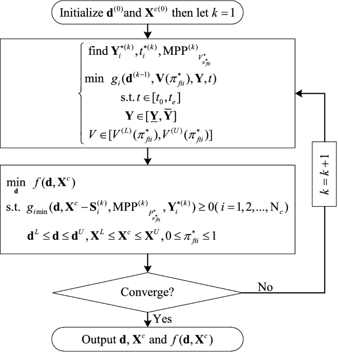

  

  Proposed series single-loop optimization procedure

• Step 3 Compute the updated design parameter solution ${\mathbf{d}}^{(k)}$, ${\mathbf{X}}^{{c(k)}}$ and the corresponding objective performance $f^{{(k)}} ({\mathbf{d}}^{{(k)}} ,{\mathbf{X}}^{{c(k)}} )$ by the deterministic optimization in Eq. (16) in Fig. 2.

• Step 4 Solve the relative errors of two adjacent objective performances, i.e.,

  $\varepsilon _{f}^{{(k)}} = \left| {\frac{{f^{{(k)}} ({\mathbf{d}}^{{(k)}} ,{\mathbf{X}}^{{c(k)}} ) - f^{{(k - 1)}} ({\mathbf{d}}^{{(k - 1)}} ,{\mathbf{X}}^{{c(k - 1)}} )}}{{f^{{(k)}} ({\mathbf{d}}^{{(k)}} ,{\mathbf{X}}^{{c(k)}} )}}} \right|$. If $\varepsilon_{f}^{(k)} \le \varepsilon$, let ${\mathbf{d}} = {\mathbf{d}}^{(k)}$ and ${\mathbf{X}}^{c} = {\mathbf{X}}^{{c(k)}}$, then go to step 5. Otherwise, let $k = k + 1$ and go to step 2.

• Step 5 Output the optimized design parameter solution $({\mathbf{d}},{\mathbf{X}}^{c} )$ and the corresponding objective performance $f({\mathbf{d}},{\mathbf{X}}^{c} )$.

5 Applications

This section is dedicated to the validation and assessment of the proposed method. Three approaches involving the TDFP-index-based method with DLOM, SLOM, and extreme value combined performance measure approach are employed to be references. In this paper, the optimization problems solved in DLOM, SLOM, EVCPMA, and SSLO method are performed with Sequential Quadratic Programming (SQP) algorithm (Belegundu and Arora 1984). An available executable program of the SQP method has been provided by the MATLAB 2018b, which is embedded in the optimizer FIMINCON. It is employed as an optimization tool in this paper. In all examples, a finite difference method is used for derivative evaluations.

5.1 Numerical example 1

Considering the following tRBDO mathematical formulation:

$$\begin{array}{*{20}l} {{\text{find}}} & {X_{1}^{c} ,X_{2}^{c} } \\ {\min } & {f({\mathbf{X}}^{c} ) = X_{1}^{c} + X_{2}^{c} } \\ {\text{s.t.}} & {{\text{poss}}\{ g_{i} ({\mathbf{X}},Y,t) \le 0,\exists t \in [t_{s} ,t_{e} ]\} \le \pi_{fti}^{ * } (i = 1,2,3)} \\ {\text{where }} & { \, g_{1} ({\mathbf{X}},Y,t) = X_{1}^{2} X_{2} - 5X_{1} t + (X_{2} + 1)t^{2} + Y - 20} \\ {} & {g_{2} ({\mathbf{X}},Y,t) = \frac{{(X_{1} + X_{2} + Y - 0.1t - 5)^{2} }}{30} + \frac{{(X_{1} - X_{2} - Y + 0.2t - 12)^{2} }}{120} - 1} \\ {} & {g_{3} ({\mathbf{X}},Y,t) = \frac{90}{{(X_{1} + 0.05t)^{2} + 8(X_{2} + 0.1t) - \sin t + 5}} + Y - 1} \\ {} & {0 \le {\mathbf{X}}^{c} \le 10,\pi_{fti}^{ * } = 0.5(i = 1,2,3)} \\ \end{array} ,$$

(22)

where two fuzzy design parameters $X_{1}$ and $X_{2}$ are fuzzy Gaussian distribution with the standard deviation $\sigma_{{X_{i} }} = 0.6$ $(i = 1,2)$, i.e., $u_{{X_{1} }} (x_{1} ) = \exp \left[ { - \left( {\frac{{x_{1} - x_{1}^{c} }}{{\sqrt 2 \sigma_{{X_{1} }} }}^{2} } \right)} \right]$ and $u_{{X_{2} }} (x_{2} ) = \exp [ - (\frac{{x_{2} - x_{2}^{c} }}{{\sqrt 2 \sigma_{{X_{2} }} }})^{2} ]$, interval variable $Y$ is bounded in $[ - 0.1,0.1]$.

The specified time interval is $[0,5]$ and the target TDFP value is 0.5 for these three constraints.

The design parameter solutions estimated by TDFP-index-based approach with DLOM and SLOM, extreme value combined performance measure approach (EVCPMA), and SSLO are shown in Table 1, in which the corresponding computational cost is also provided. It should be noted that the computational cost in the Table 1 involves all the necessary estimation of the constraint functions. The final TDFP index statistics of these methods are also represented in Table 2. The initial design parameters are set to be $[X_{1}^{c} ,X_{2}^{c} ] = [5,5]$ for all these methods. Figure 3 illustrates the constraint situations in the original fuzzy space in the entire optimization process, and the initial design parameters $[X_{1}^{c} ,X_{2}^{c} ] = [5,5]$ are not shown in Fig. 3.

Table 1 Summary of the optimization results for the Example 5.1

Table 2 The TDFP-index constraints at optimal design parameters of example 5.1

Fig. 3

Iteration history by SSLO of example 5.1

From Table 1, one can see that the optimal parameters addressed by the proposed SSLO can match well with that of the DLOM, SLOM, and EVCPMA representing the basic strategies, which demonstrates the accuracy of the SSLO for tRBDO. It can be found that the design parameters calculated by EVCPMA are much close to those of the proposed SSLO, but the computation cost of the EVCPMA is more than two thousands, which is almost six times of that of the proposed SSLO. The optimal solution calculated by the DLOM and SLOM need huge computational cost, especially the DLOM, which is mainly caused by the quadruple nested loop optimization. The computational statistics in Table 1 show that the calls of the objective function by the DLOM, SLOM, and EVCPAM are about 20 times and the proposed SSLO just need 5 times, which makes the proposed SSLO more efficient than other method. The reason is that the design solution shifts its optimum as quickly as possible so to reduce the needs for locating most probable point.

The optimal parameter solutions are $[X_{1}^{c} ,X_{2}^{c} ] = [3.8179,4.1798]$ solved by those methods. It can be seen from Fig. 3 that these two optimal parameters make these TDFP constraints satisfy the target safety level for SSLO. It can be seen from Fig. 3 that the design parameters are removed from the first constraint; thus, optimal solutions can make the TDFP index of first constraint satisfy the target safety level. The design solution moves to its optimum very quickly which is also shown in Fig. 3.

5.2 Numerical example 2

Let us consider the following tRBDO problem

$$\begin{array}{*{20}l} {\min } & {f({\mathbf{X}}^{c} ) = (X_{1}^{c} - 3.7)^{2} + (X_{2}^{c} - 4)^{2} } \\ {{\text{s}}{\text{.t}}{.}} & {P\{ g_{i} ({\mathbf{X}},t) \le 0\exists t \in [t_{s} ,t_{e} ]\} \le \pi_{fti}^{ * } (i = 1,2)} \\ {} & {g_{1} ({\mathbf{X}},t) = - X_{1} \sin (4X_{1} ) - 1.1X_{2} \sin (2X_{2} ) + 1.2t} \\ {} & {g_{2} ({\mathbf{X}},t) = X_{1} + X_{2} - 3t} \\ {} & {0 \le X_{1}^{c} \le 3.7,0 \le X_{2}^{c} \le 4,\pi_{fti}^{ * } = 0.5(i = 1,2)} \\ \end{array} ,$$

(23)

where the fuzzy design parameter $X_{i} (i = 1,2)$ is triangle fuzzy distribution, whose membership function is expressed by $u_{{X_{i} }} (x_{i} ) = \left\{ {\begin{array}{*{20}l} {1 + {{(x_{i} - x_{i}^{c} )} \mathord{\left/ {\vphantom {{(x_{i} - x_{i}^{c} )} {0.3}}} \right. \kern-\nulldelimiterspace} {0.3}}} \\ {1 - {{(x_{i} - x_{i}^{c} )} \mathord{\left/ {\vphantom {{(x_{i} - x_{i}^{c} )} {0.3}}} \right. \kern-\nulldelimiterspace} {0.3}}} \\ \end{array} } \right.$, and the considered time interval is $t \in [0,1]$.

The initial design parameter in the numerical example 2 is $[X_{1}^{c} ,X_{2}^{c} ] = [3,3]$. The optimal design parameter solutions estimated by DLOM, SLOM, and EVCPMA are listed in Table 3, which can match well with that of SSLO. This demonstrates the accuracy of three methods in solving tRBDO problems. As is shown in Table 3, the number of function calls of the DLOM and SLOM are extremely high, which is impractical for engineering application, while the function calls of SSLO is fewer than the EVCPMA. Therefore, the proposed SSLO method is efficient and accurate for solving the tRBDO problems.

Table 3 Summary of the optimization results for the Example 5.1

From the Table 4, we can conclude that the first constraint is active, while the second constraint is inactive. The TDFP of the optimal parameters estimated by DLOM, SLOM, EVCPMA, and SSLO fulfill the target TDFP. Thus, the proposed method is more efficient than other methods.

Table 4 The TDFP index constraints at optimal design parameters of example 5.1

5.3 Two bars frame

Let us consider the two bar frame shown in Fig. 4 already studied in reference (Hu and Du 2016; Shi et al. 2020a). The frame is subjected to a dynamic force $F(t) = F_{0} \sin (t)$. The yield strength of the two bars degenerates over time, i.e., $S_{1} (t) = S_{01} \exp ( - 0.01t)$ and $S_{2} (t) = S_{02} \exp ( - 0.01t)$, in which $S_{01}$ and $S_{02}$ are the initial yield strengths of two bars, respectively. The structural failure is defined as the maximum stress of the bar higher than the corresponding yield strength, and the objective is to minimize the weight of this frame work. The tRBDO of this two bars frame is formulated as follows:

$$\begin{array}{*{20}l} {\min } \hfill & {f(d) = \frac{{\pi l_{1} X_{{D_{1} }}^{{c^{2} }} + \pi \sqrt {l_{1}^{2} + l_{2}^{2} X_{{D_{2} }}^{{c^{2} }} } }}{4}} \hfill \\ {{\text{s.t.}}} \hfill & {{\text{poss}}\{ g_{i} ({\mathbf{Z}},t) \le 0,\exists t \in [t_{s} ,t_{e} ]\} \le \pi _{{fti}}^{*} (i = 1,2)} \hfill \\ {} \hfill & {g_{1} ({\mathbf{Z}},t) = 1 - \frac{{4F(t)\sqrt {l_{1}^{2} + l_{2}^{2} } }}{{\pi l_{2} D_{1}^{2} S_{1} (t)}}} \hfill \\ {} \hfill & {g_{2} ({\mathbf{Z}},t) = 1 - \frac{{4F(t)l_{1} }}{{\pi l_{2} D_{2}^{2} S_{2} (t)}}} \hfill \\ {} \hfill & {{\mathbf{Z}} = [{\mathbf{X}},{\mathbf{P}}],{\mathbf{X}} = [D_{1} ,D_{2} ],{\mathbf{P}} = [S_{{01}} ,S_{{02}} ,l_{1} ,l_{2} ,F_{0} ]} \hfill \\ {} \hfill & {0.07\;{\text{m}} \le X_{{D_{i} }}^{c} \le 0.25\;{\text{m}},\pi _{{fti}}^{*} = 0.4(i = 1,2)} \hfill \\ \end{array} ,$$

(24)

where $t \in [0,10]$ year.

Fig. 4

Two bar frame

Distribution parameters of the input variables are listed in Table 5.

Table 5 Distribution parameters of the fuzzy input variable vector of Example 5.2

In this example, the fuzzy design vector, the fuzzy parameter vector, and the time parameter are involved in the constraint functions. The initial design parameters are set to be $[X_{{D_{1} }}^{c} ,X_{{D_{2} }}^{c} ] = [0.15,0.15]$ for all these methods. The design parameter solutions and computational statistics calculated by TDFP-index-based method with DLOM and SLOM, EVCPMA, and SSLO are listed in Table 6. The final TDFP indexes of these methods are shown in Table 7.

Table 6 Summary of the optimization results for the Example 5.2

Table 7 The TDFP-index constraints at optimal design parameters of example 5.2

The optimal solutions of the two bars frame shown in Table 6 demonstrate again that the SSLO is an accurate algorithm to compute the tRBDO with fuzzy and interval uncertainties. Strictly speaking, the design parameter solutions estimated by the TDFP-index-based approach with DLOM and SLOM have little errors, because the final TDFP of the constraint is less than the target safety level. The optimal solutions illustrate that the parameters $[X_{{D_{1} }}^{c} ,X_{{D_{2} }}^{c} ] = [0.1741,0.1561]$ of the two bars frame can guarantee the given safety degree under the dynamic force $F(t)$. According to the definition of the TDFP, if the values of dimensional parameters are bigger than the optimal solutions, the TDFP of constraints will larger than the target safety degree, but material waste will be made under this situation; therefore, the optimal solutions can simultaneously balance cost and safety. The comparison of the numbers of the function calls for different methods in Table 6 and demonstrates the efficiency of the SSLO.

5.4 A three-bar truss structure

A three-bar truss structure shown in Fig. 5 is considered. The cross-sectional area of truss 2 is denoted by $A_{2}$ with the length $L = 50.8\;{\text{cm}}$. Truss 1 and 3 has the same length and cross-sectional area which are $\sqrt 2 L$ and $A_{1}$ , respectively. The density and elastic modulus of the material are $\rho = 2.768 \times 10^{ - 3} {\text{kg/cm}}^{{3}}$ and $E = 6.895 \times 10^{3} {\text{kN/cm}}^{{2}}$. The load $P$ applied on the node 4, the strengths of three trusses are degenerated over time, i.e., $\sigma_{t} = \sigma_{0t} \exp ( - 0.01t)$ and $\sigma_{c} = \sigma_{0c} \exp ( - 0.01t)$, allowable horizontal and vertical displacements ($u_{4}$ and $v_{4}$) are fuzzy parameter variables, the frame is subjected to a dynamic force $P = P_{0} \sin t$. The design objective is to minimize the total weight of the three-bar structure and cross-sectional areas are treated as fuzzy design variables, with the lower bound as 0.64516 cm². It is assumed that variables are all Gaussian fuzzy sets, and the distribution parameters are shown in Table 8. The tRBDO of this three bars frame is formulated as follows:

$$\begin{array}{*{20}l} {\min } & {f(d) = \rho L(2\sqrt 2 X_{{A_{1} }}^{c} + X_{{A_{2} }}^{c} )} \\ {{\text{s.t.}}} & {{\text{poss}}\{ g_{i} ({\mathbf{Z}},t) \le 0,\exists t \in [t_{0} ,t_{e} ]\} \le \pi_{fti}^{ * } (i = 1,2, \ldots ,5)} \\ {} & {g_{1} ({\mathbf{Z}},t) = u_{4} - \frac{\sqrt 2 PL\cos \theta }{{A_{1} E}}} \\ {} & {g_{2} ({\mathbf{Z}},t) = v_{4} - \frac{\sqrt 2 PL\sin \theta }{{(A_{1} + \sqrt {A_{2} } )E}}} \\ {} & {g_{3} ({\mathbf{Z}},t) = \sigma_{t} - \frac{\sqrt 2 }{2}\left( {\frac{P\cos \theta }{{A_{1} }} + \frac{P\sin \theta }{{A_{1} + 2\sqrt {A_{2} } }}} \right)} \\ {} & {g_{4} ({\mathbf{Z}},t) = \sigma_{t} - \frac{\sqrt 2 P\sin \theta }{{A_{1} + 2\sqrt {A_{2} } }}} \\ {} & {g_{5} ({\mathbf{Z}},t) = \sigma_{c} - \frac{\sqrt 2 }{2}\left( {\frac{P\cos \theta }{{A_{1} }} + \frac{P\sin \theta }{{A_{1} + 2\sqrt {A_{2} } }}} \right)} \\ {} & {{\mathbf{Z}} = [{\mathbf{X}},{\mathbf{P}}],{\mathbf{X}} = [A_{1} ,A_{2} ],{\mathbf{P}} = [P,u_{4} ,v_{4} ,\sigma_{t} ,\sigma_{c} ]} \\ {} & {0.64516 \le X_{{A_{i} }}^{c} ,\pi_{fti}^{ * } = 0.4(i = 1,2)} \\ \end{array} ,$$

(25)

Fig. 5

Three-bar truss structure

Table 8 Distribution parameters of the fuzzy input variable vector of Example 5.3

The initial design parameters are set to be $[X_{{A_{1} }}^{c} ,X_{{A_{2} }}^{c} ] = [80,20]$ for all these methods. The design parameter solutions and computational statistics calculated by DLOM, SLOM, EVCPMA, and SSLO are listed in Table 9. The final TDFP indexes of these methods are listed in Table 10.

Table 9 Summary of the optimization results for the Example 5.3

Table 10 The TDFP-index constraints at optimal design parameters of example 5.3

The optimal solutions of the three bars frame listed in Table 9 show that the SSLO closely meets other algorithms. The optimal solutions demonstrate that the design parameters $[X_{{A_{1} }}^{c} ,X_{{A_{2} }}^{c} ] = [72.3004,18.6553]$ of the three bars frame can hold the target safety degree under the external load $P$ which is listed in Table 10. From Table 10, the fourth and fifth constraints are inactive. The comparison of the number of the function calls demonstrates that the SSLO is an accurate and efficient method.

5.5 A welded beam with a time-dependent force

A welded beam shown in Fig. 6 is subjected to a time-dependent loading $F(t) = F_{0} \sin t$ in the right end of this beam (Jiang et al. 2017; Shi et al. 2020b), and the left end of this beam is welded. The fuzzy design variable vector is relative to the welding point containing it’s depth $X_{1}$, length $X_{2}$, height $X_{3}$ , and thickness $X_{4}$. A time-independent possibility constraint function and four time-dependent possibility constraint functions are introduced in this optimization problem, in which the time-independent possibility constraint function is the restriction of welding size, and four time-dependent possibility constraint functions referred to the shear stress, bucking, bending stress and the displacement of free end. The objective function is to minimize the cost of welding. The random parameters are the young’s Modulus $E$, the length of this beam $L$, the shear Modulus $G$, the allowable displacement of free end $d_{0}$, and maximum shear stress $\tau$ , and the maximum normal stress $\sigma$. The tRBDO of this welded beam is constructed as follows.

$$\begin{array}{*{20}l} {{\text{find}}} & {{\mathbf{d}}{\text{ = [X}}_{1}^{c} {\text{,X}}_{2}^{c} {\text{,X}}_{3}^{c} {\text{,X}}_{4}^{c} {]}} \\ {{\text{min}}} & {f({\mathbf{X}}^{c} ) = c_{1} X_{1}^{c} X_{2}^{c} + c_{2} X_{3}^{c} X_{4}^{c} (L + X_{2}^{c} )} \\ {\text{s.t.}} & {{\text{poss}}\{ g_{i} ({\mathbf{Z}},t) \le 0,\exists t \in [0,10]\} \le \underline {\pi }_{fti} (i = 1,2,4,5)} \\ {} & {{\text{poss}}\{ g_{3} ({\mathbf{Z}}) \le 0\} \le \underline {\pi }_{f} } \\ {} & {{\mathbf{Z}} = [{\mathbf{X}},{\mathbf{P}}],{\mathbf{X}} = [X_{1} ,X_{2} ,X_{3} ,X_{4} ],{\mathbf{P}} = [E,L,G,d,\tau ,\sigma ,F_{0} ]} \\ {} & {3.175 \le X_{1}^{c} \le 50.8,X_{2}^{c} \le 254,X_{3}^{c} \le 254,X_{4}^{c} \le 50.8} \\ {} & {\pi_{fti}^{ * } = 0.5(i = 1,2,4,5),\pi_{f}^{ * } = 0.5,[t_{0} ,t_{e} ] = [0,10]{\text{year}}} \\ \end{array} ,$$

(26)

$$\begin{aligned} {\text{where }}g_{1} ({\mathbf{Z}},t) = & 1 - \frac{{\tau ({\mathbf{Y}},t)}}{\tau },g_{2} ({\mathbf{Z}},t) = 1 - \frac{{\sigma ({\mathbf{Z}},t)}}{\sigma } \\ g_{3} ({\mathbf{Z}}) = & 1 - \frac{{X_{1} }}{{X_{4} }},g_{4} ({\mathbf{Z}},t) = 1 - \frac{{\delta ({\mathbf{Z}},t)}}{{d_{0} }} \\ g_{5} ({\mathbf{Z}},t) = & \frac{{P_{c} ({\mathbf{Z}})}}{F} - 1 \\ \tau ({\mathbf{Z}},t) = & \sqrt {L^{2} ({\mathbf{Z}},t) + \frac{{2L({\mathbf{Z}},t)S({\mathbf{Z}},t)X_{2} }}{{2R({\mathbf{Z}})}} + S^{2} ({\mathbf{Z}},t)} \\ L({\mathbf{Z}},t) = & \frac{F}{{\sqrt 2 X_{1} X_{2} }},S({\mathbf{Z}},t) = \frac{{M({\mathbf{Z}},t)R({\mathbf{Z}})}}{{J({\mathbf{Z}})}} \\ M({\mathbf{Z}},t) = & F(L + 0.5X_{2} ),\delta ({\mathbf{Z}},t) = \frac{{4FL^{3} }}{{EX_{3}^{3} X_{4} }} \\ R({\mathbf{Z}}) = & 0.5\sqrt {X_{2}^{2} + (X_{1} + X_{3} )^{2} } ,J({\mathbf{Z}}) = \sqrt 2 X_{1} X_{2} \left[ {\frac{{X_{2}^{2} }}{12} + \frac{{(X_{1} + X_{3} )^{2} }}{4}} \right] \\ \sigma ({\mathbf{Z}},t) = & \frac{6FL}{{X_{3}^{2} X_{4} }},P_{c} ({\mathbf{Z}}) = \frac{{4.013X_{3} X_{4}^{3} \sqrt {EG} }}{{6L^{2} }}\left( {1 - \frac{{X_{3} }}{4L}\sqrt{\frac{E}{G}} } \right) \\ \end{aligned}$$

(27)

Fig. 6

A welding beam structure

Fuzzy distribution parameters of the input variables are listed in Table 11.

Table 11 The distribution parameters of the input variables of example 5.4

In this application, the fuzzy design variables and their parameters are involved in the constraint functions. The initial design parameters are set to be ${\text{[X}}_{1}^{c} {\text{,X}}_{2}^{c} {\text{,X}}_{3}^{c} {\text{,X}}_{4}^{c} {] = [15,220,220,15]}$ for all these methods. The design parameters solved by TDFP-index-based approach with SLOM, EVCPMA, and SSLO and computational statistics are listed in Tables 12 and 13, while the DLOM cannot converge, because the TDFP analysis with DLOM traps in local optima, and the solutions of TDFP index cannot reach. The final TDFP index solutions of five constraints are listed in Table 14.

Table 12 The design parameter solution for the Example 5.4

Table 13 Number of function calls of example 5.4

Table 14 TDFP index of constraints at optimal design parameters of example 5.4

From Table 12, the conclusion can be obtained that the design parameter solutions calculated by the TDFP-index-based approach with SLOM, EVCPMA, and SSLO are almost the same with each other. From Table 14, it is easy to find that all the TDFP index of constraints with the parameter solutions addressed by the proposed method can match well with the target safety level, while the TDFP index of the third and fourth constraints with the optimal parameters calculated by the SLOM do not match the target safety level very well. It is shown in Table 13 that the calls of the objective function are only 9 times and the calls of the constraints are 1675 times. In a word, the established tRBDO under the fuzzy and interval uncertainties is rational and the proposed SSLO method is efficient in solving tRBDO.

5.6 A wing reinforcing rib

The design of the wing reinforcing rib demonstrated in Fig. 7 is modified to illustrate the effectiveness of the proposed SSLO. Six round holes are punched in the middle of the reinforcing rib, which are represented by A, B, C, D, E and F respectively that is demonstrated in Fig. 8. the largest hole represented by A is used to fix the engine which generates the torque to retract slat, and the top hole represented by B is performed to insert pipes and cables, and the remaining four holes represented by C, D, E and F respectively are performed to support the slide rails for retracting the slat. The radius of these holes is fuzzy variables and the mean of these variables is design parameters, which are represented by $A^{c}$, $B^{c}$, $C^{c}$, $D^{c}$, $E^{c}$ and $F^{c}$ respectively. The thickness of the reinforcing rib $d$, the elastic modulus E, aerodynamic pressure $P_{1}$ and $P_{2}$, concentrated loads $F_{1}$, $F_{2}$, $F_{3}$, $F_{4}$ are supposed as fuzzy variables. The loads $F_{5} (t) = F_{5} \sin t$ and $F_{6} (t) = F_{6} \sin t$ are time-dependent variables. The failure state of the rib corresponds to that the maximum longitudinal displacement $\Delta d_{\max }$ or maximum principal stress $S_{\max }$ exceeds the specified thresholds. The optimization objective is to minimize the structural weight, therefore maximize the sum of squares of radius of these holes. The tRBDO of the wing reinforcing rib is expressed as follows:

$$\begin{array}{*{20}l} {\mathop {\max }\limits_{{R^{c} }} } \hfill & {f(R^{c} ) = R_{A}^{{c^{2} }} + R_{B}^{{c^{2} }} + R_{C}^{{c^{2} }} + R_{D}^{{c^{2} }} + R_{E}^{{c^{2} }} + R_{F}^{{c^{2} }} } \hfill \\ {{\text{s.t.}}} \hfill & {{\text{poss}}\{ g_{i} ({\mathbf{Z}},Y,t,\Delta d_{{{\text{allow}}}} ,S_{{{\text{allow}}}} ) \le 0{\mkern 1mu} \exists t \in [0,12]\} \le \underset{\raise0.3em\hbox{$\smash{\scriptscriptstyle-}$}}{\pi } _{{fti}} (i = 1,2){\mkern 1mu} } \hfill \\ {} \hfill & {{\text{g}}_{1} (Z,d,t,\Delta d_{{{\text{allow}}}} ) = \Delta d_{{{\text{allow}}}} - \Delta d_{{\max }} (R_{A} ,R_{B} ,R_{C} ,R_{D} ,R_{E} ,R_{F} ,d,} \hfill \\ {} \hfill & {E,P_{1} ,P_{2} ,F_{1} ,F_{2} ,F_{3} ,F_{4} ,F_{5} (t),F_{6} (t))} \hfill \\ {} \hfill & {{\text{g}}_{2} (Z,d,t,S_{{{\text{allow}}}} ) = S_{{{\text{allow}}}} - S_{{\max }} (R_{A} ,R_{B} ,R_{C} ,R_{D} ,R_{E} ,R_{F} ,d,} \hfill \\ {} \hfill & {E,P_{1} ,P_{2} ,F_{1} ,F_{2} ,F_{3} ,F_{4} ,F_{5} (t),F_{6} (t))} \hfill \\ {} \hfill & {\pi _{{fti}}^{*} = 0.5(i = 1,2),\Delta d_{{{\text{allow}}}} = 0.075\exp ( - 0.01t),S_{{{\text{allow}}}} = 55000\exp ( - 0.02t)} \hfill \\ {} \hfill & {30.{\text{0}}\;{\text{mm}} \le R_{A}^{c} \le 36.0\;{\text{mm}},18.{\text{5}}\;{\text{mm}} \le R_{B}^{c} \le 21.5\;{\text{mm}}} \hfill \\ {} \hfill & {7.{\text{9}}\;{\text{mm}} \le R_{C}^{c} \le 9.0\;{\text{mm}},7.{\text{9}}\;{\text{mm}} \le R_{D}^{c} \le 9.0\;{\text{mm}}} \hfill \\ {} \hfill & {7.{\text{9}}\;{\text{mm}} \le R_{E}^{c} \le 9.0\;{\text{mm}},7.{\text{9}}\;{\text{mm}} \le R_{F}^{c} \le 9.0\;{\text{mm}}} \hfill \\ \end{array}$$

(28)

Fig. 7

The wing reinforcing rib of a civil aircraft

Fig. 8

The diagram of the reinforcing rib

Distribution parameters of these inputs are illustrated in Table 15. The finite element models of the reinforcing rib with respect to longitudinal displacement and principal stress are illustrated in Fig. 9.

Table 15 Distribution parameters of the inputs of example 5.5

Fig. 9

The finite element models of the reinforcing rib

The design parameter solutions estimated by EVCPMA and SSLO are listed in Table 16 because it needs huge computational cost to solve this engineering application by using DLOM and SLOM; thus, we only provide the solutions estimated by the EVCPMA and SSLO methods. Anyhow, the effectiveness of the proposed SSLO can be shown by comparing with EVCPMA, and the target failure possibility solutions evaluated based on the real finite element model are provided inside parentheses.

Table 16 The design parameter solution for the Example 5.5

As is shown in Table 16, one can see that the design parameters solved by EVCPMA and SSLO have similar accuracy. Table 17 shows that the proposed SSLO is the most efficient one among these methods, which requires 4154 times calls of the constraints functions, while the EVCPMA requires 12,358 times calls of the constraints functions. Therefore, the efficiency of the proposed SSLO is demonstrated. From Table 18, the target failure possibility solutions illustrate that the first constraint is active and the second constraint is inactive, and the final TDFP fulfills the target failure possibility. In a word, the accuracy and the efficiency of the proposed SSLO method are proved in all examples.

Table 17 Number of function calls of example 5.5

Table 18 TDFP index of constraints at optimal design parameters of example 5.5

6 Conclusions

The TDFP index can accurately measure the safety degree of the time-dependent structure under the fuzzy and interval uncertainties, and the tRBDO based on TDFP index is established to solve the optimal design parameters with the TDFP constraints. The tRBDO with both fuzzy and interval uncertainties is time-consuming in engineering practice and generally needs huge computational burden. An efficient estimation strategy named SSLO is established to solve the tRBDO with both fuzzy and interval uncertainties. In our strategy, the deterministic optimization, time instant, and interval value estimations corresponding to the worst case scenario and most probable point searching are alternately performed to obtain the optimal design parameters. Our strategy avoids the triple-loop estimation process in the original tRBDO with fuzzy and interval uncertainties by the TDFP-index-based approach for cost-consuming engineering problems; thus, it can save computational cost. Two vital points in our strategy guarantee its high efficiency. One is that no iterative searching step is needed to find the most probable point at each iteration step. The other one is that the time instant, interval value estimations corresponding to the worst case scenario, and most probable point are solved with single-loop optimization, which can improve the efficiency of the proposed SSLO method.

Several numerical and engineering examples are introduced to show the effectiveness of the proposed SSLO. The solutions demonstrate that the established tRBDO under the fuzzy and interval uncertainties is rational, and the proposed SSLO method is accurate and efficient in solving the tRBDO. Simultaneously, the proposed SSLO is robust in various examples, and this kind of method is firstly introduced to solve tRBDO involving fuzzy and interval uncertainties. It should be noted that one key point of the established SSLO is based on the optimization, for the problem with large dimensionality and highly nonlinearity, optimization based method may introduce big computational demand. Therefore, the established SSLO is suitable for the problem with small or moderate dimensionality and nonlinearity. Dealing with the tRBDO under fuzzy and interval uncertainties with large dimensionality and highly nonlinearity will be our future focus, and the meta-model can deal with high nonlinear and dimensional engineering problem in tRBDO. Machine learning techniques, such as Kriging/Gaussian process, support vector machine, neural networks, and polynomial chaos expansion, can approximate realistic engineering high nonlinear and dimensional problems, i.e., FEM problem. The active learning algorithm only needs few training samples to get accurate explicit performance function. Finally, the proposed method can deal with the explicit function efficiently.

References

Belegundu AD, Arora JS (1984) A recursive quadratic programming method with active set strategy for optimal design. Int J Numer Methods Eng 20:803–816. https://doi.org/10.1002/nme.1620200503
Cremona C, Gao Y (1997) The possibilistic reliability theory: theoretical aspects and applications. Struct Saf 19:173–201
Du X, Chen W (2004) Sequential optimization and reliability assessment method for efficient probabilistic design. J Mech Des Trans ASME 126:225–233. https://doi.org/10.1115/1.1649968
Du L, Choi KK (2008) An inverse analysis method for design optimization with both statistical and fuzzy uncertainties, Struct Multidisc Optim 37(2):107–119. https://doi.org/10.1007/s00158-007-0225-0.
Du L, Choi KK, Youn BD (2006) Inverse possibility analysis method for possibility-based design optimization. AIAA J 44:2682–2690. https://doi.org/10.2514/1.16546
Dubois D, Prade H (1987) The mean value of a fuzzy number. Fuzzy Sets Syst 24:279–300. https://doi.org/10.1016/0165-0114(87)90028-5
Elishakoff I, Ferracuti B (2006) Fuzzy sets based interpretation of the safety factor. Fuzzy Sets Syst 157:2495–2512
Fan C, Lu Z, Shi Y (2018) Safety life analysis under the required failure possibility constraint for structure involving fuzzy uncertainty. Struct Multidisc Optim 58:287–303. https://doi.org/10.1007/s00158-017-1896-9
Fan C, Lu Z, Shi Y (2019) Time-dependent failure possibility analysis under consideration of fuzzy uncertainty. Fuzzy Sets Syst 367:19–35. https://doi.org/10.1016/j.fss.2018.06.016
Graf W, Beer M, Mo B (2000) Fuzzy structural analysis using a -level optimization, Comput Mech 26(6):547–565
Hao P, Wang Y, Liu C, Wang B, Wu H (2017) A novel non-probabilistic reliability-based design optimization algorithm using enhanced chaos control method. Comput Methods Appl Mech Eng 318:572–593. https://doi.org/10.1016/j.cma.2017.01.037
Hu Z, Du X (2016) Reliability-based design optimization under stationary stochastic process loads. Eng Optim 48:1296–1312. https://doi.org/10.1080/0305215X.2015.1100956
Hu Y, Lu Z, Wei N, Zhou C (2020) A single-loop Kriging surrogate model method by considering the first failure instant for time-dependent reliability analysis and safety lifetime analysis. Mech Syst Signal Process 145:106963. https://doi.org/10.1016/j.ymssp.2020.106963
Huang ZL, Jiang C, Zhou YS, Luo Z, Zhang Z (2016) An incremental shifting vector approach for reliability-based design optimization. Struct Multidisc Optim 53:523–543. https://doi.org/10.1007/s00158-015-1352-7
Jia B, Lu Z, Wang L (2020) A decoupled credibility-based design optimization method for fuzzy design variables by failure credibility surrogate modeling. Struct Multidisc Optim 62:285–297. https://doi.org/10.1007/s00158-020-02487-6
Jiang C, Fang T, Wang ZX, Wei XP, Huang ZL (2017) A general solution framework for time-variant reliability based design optimization. Comput Methods Appl Mech Eng 323:330–352. https://doi.org/10.1016/j.cma.2017.04.029
Jiang C, Han X, Liu GR (2007) Optimization of structures with uncertain constraints based on convex model and satisfaction degree of interval. Comput Methods Appl Mech Eng 196:4791–4800. https://doi.org/10.1016/j.cma.2007.03.024
Kang Z, Luo Y, Li A (2011) On non-probabilistic reliability-based design optimization of structures with uncertain-but-bounded parameters. Struct Saf 33:196–205. https://doi.org/10.1016/j.strusafe.2011.03.002
Keshtegar B, Hao P (2018) A hybrid descent mean value for accurate and efficient performance measure approach of reliability-based design optimization. Comput Methods Appl Mech Eng 336:237–259. https://doi.org/10.1016/j.cma.2018.03.006
Ling C, Lu Z, Sun B, Wang M (2019) An efficient method combining active learning Kriging and Monte Carlo simulation for profust failure probability. Fuzzy Sets Syst 1:1–19. https://doi.org/10.1016/j.fss.2019.02.003
Meng Z, Keshtegar B (2019) Adaptive conjugate single-loop method for efficient reliability-based design and topology optimization. Comput Methods Appl Mech Eng 344:95–119. https://doi.org/10.1016/j.cma.2018.10.009
Mourelatos ZP, Zhou J (2005) Reliability estimation and design with insufficient data based on possibility theory. AIAA J 43:1696–1705. https://doi.org/10.2514/1.12044
Royset JO, Der Kiureghian A, Polak E (2001) Reliability-based optimal structural design by the decoupling approach. Reliab Eng Syst Saf 73:213–221. https://doi.org/10.1016/S0951-8320(01)00048-5
Schuëller GI, Jensen HA (2008) Computational methods in optimization considering uncertainties: an overview. Comput Methods Appl Mech Eng 198:2–13. https://doi.org/10.1016/j.cma.2008.05.004
Shi Y, Lu Z, Huang Z, Xu L, He R (2020a) Advanced solution strategies for time-dependent reliability based design optimization. Comput Methods Appl Mech Eng 364:112916. https://doi.org/10.1016/j.cma.2020.112916
Shi Y, Lu Z, Xu L, Zhou Y (2020b) Novel decoupling method for time-dependent reliability-based design optimization. Struct Multidisc Optim 61:507–524. https://doi.org/10.1007/s00158-019-02371-y
Tang ZC, Lu ZZ, Hu JX (2014) An efficient approach for design optimization of structures involving fuzzy variables. Fuzzy Sets Syst 255:52–73. https://doi.org/10.1016/j.fss.2014.05.017
Tu J, Choi KK, Park YH (1999) A new study on reliability- based design optimization. J Mech Des Trans ASME 121:557–564. https://doi.org/10.1115/1.2829499
Wang L, Lu Z, Jia B (2020) A decoupled method for credibility-based design optimization with fuzzy variables. Int J Fuzzy Syst 22:844–858. https://doi.org/10.1007/s40815-020-00813-0
Wang C, Qiu Z, Xu M, Li Y (2017) Novel reliability-based optimization method for thermal structure with hybrid random, interval and fuzzy parameters. Appl Math Model 47:573–586. https://doi.org/10.1016/j.apm.2017.03.053
Wang L, Ren Q, Ma Y, Wu D (2019b) Optimal maintenance design-oriented nonprobabilistic reliability methodology for existing structures under static and dynamic mixed uncertainties. IEEE Trans Reliab 68:496–513. https://doi.org/10.1109/TR.2018.2868773
Wang L, Xiong C (2019) A novel methodology of sequential optimization and non-probabilistic time-dependent reliability analysis for multidisciplinary systems. Aerosp Sci Technol 94:105389. https://doi.org/10.1016/j.ast.2019.105389
Wang L, Xiong C, Wang X, Liu G, Shi Q (2019a) Sequential optimization and fuzzy reliability analysis for multidisciplinary systems. Struct Multidisc Optim 60:1079–1095. https://doi.org/10.1007/s00158-019-02258-y
Xiong C, Wang L, Liu G, Shi Q (2019) An iterative dimension-by-dimension method for structural interval response prediction with multidimensional uncertain variables. Aerosp Sci Technol 86:572–581. https://doi.org/10.1016/j.ast.2019.01.032
Yao W, Chen X, Luo W, Van Tooren M, Guo J (2011) Review of uncertainty-based multidisciplinary design optimization methods for aerospace vehicles. Prog Aerosp Sci 47:450–479. https://doi.org/10.1016/j.paerosci.2011.05.001
Zadeh LA (1965) Fuzzy Sets. Inf Control 8:338–353
Zhang J, Taflanidis AA, Medina JC (2017) Sequential approximate optimization for design under uncertainty problems utilizing Kriging metamodeling in augmented input space. Comput Methods Appl Mech Eng 315:369–395. https://doi.org/10.1016/j.cma.2016.10.042
Acknowledgements
This work was supported by the Special Scientific Research Project of Education Department of Shaanxi Province (No. 20JK0731), the China Scholarship Council (No. 202108610168), and Shaanxi Natural Science Foundation General Program (No. 2020JM-481).
Author information
Authors and Affiliations
Corresponding author
Ethics declarations
Conflict of interest
The author declares to have no conflict of interest.
Replication of results
For replication of the results of all test examples, the main MATLAB codes have been uploaded as the supplementary material. The reader can change the response function and the input variables in the corresponding source codes to reproduce the results of all cases shown in the manuscript.
Additional information
Responsible Editor: Yoojeong Noh
Publisher's Note
Springer Nature remains neutral with regard to jurisdictional claims in published maps and institutional affiliations.
Rights and permissions
About this article
Cite this article
Fan, C., Shi, Y., Li, L. et al. Advanced solution framework for time-dependent reliability-based design optimization under fuzzy and interval uncertainties. Struct Multidisc Optim 65, 25 (2022). https://doi.org/10.1007/s00158-021-03142-4
Received:
Revised:
Accepted:
Published:
DOI: https://doi.org/10.1007/s00158-021-03142-4