Stokes’ first problem for a thermoelectric Newtonian fluid

Abstract

This work is related to the flow of an electro-conducting Newtonian fluid presenting thermoelectric properties in the presence of magnetic field. The flow is considered to be governed an incompressible viscous fluid. The electro-conducting thermofluid equation heat transfer with one relaxation time is derived. The state space formulation developed in Ezzat (Can. J. Phys. Rev. 86:1242–1450, 2008) or one-dimensional problems is introduced. The Laplace transform technique is used. The resulting formulation is applied to a thermal shock problem; that is, a problem of a layer media and a problem for the infinite space in the presence of heat sources. A numerical method is employed for the inversion of the Laplace transforms. Numerical results are given and illustrated graphically for each problem. The effects of thermoelastic properties on the thermofluid flow are studied.

1 Introduction

Thermoelectric currents in the presence of magnetic fields can cause pumping or stirring of liquid-metal coolants in nuclear reactors or stirring of molten metal in industrial metallurgy. The interaction between the thermal and MHD fields is a mutual one owing to alterations in the thermal convection and to the Peltier and Thomson effects (although these are usually small) [2].

During the 1990s there was a heightened interest in the field of thermoelectrics driven by the need for more efficient materials for electronic refrigeration and power generation [3]. Proposed industrial and military applications of thermoelectric materials are generating an increasing activity in this field by demanding a higher performance, near room-temperature thermoelectric materials than those presently in use.

A direct conversion between electricity and heat by using thermoelectric materials has attracted much attention because of their potential applications in Peltier coolers and thermoelectric power generators [4]. Thermoelectric devices have many attractive features compared with the conventional fluid-based refrigerators and power generation technologies, such as long life, unmoving parts, no noise, easy maintenance and high reliability. However, their use has been limited by the relatively low performance of present thermoelectric materials. The efficiency of a thermoelectric material is related to the so-called dimensionless thermoelectric figure-of-merit ZT. The thermoelectric figure of merit provides a measure of the quality of such materials for applications and is defined in [5]:

$$ \mathit{ZT} = \frac{\sigma_{o}S^{2}}{\kappa} T, $$

(1)

where S is the Seebeck coefficient, σ _o the electrical conductivity, T the absolute temperature, and κ is the thermal conductivity. The best thermoelectric materials that are currently in devices have a value of ZT≈1. This value, ZT≈1, has been a practical upper limit since the 1970s, yet no theoretical or thermodynamic reason exists for a ZT≈1, as an upper barrier. A good thermoelectric material has a high ZT value at the operating temperature. Materials with ZT>1 are expected to be competitive against other methods of refrigeration and electric power generation. Bismuth telluride based alloys showing ZT values of approximately 1.0 at room temperature [6] have been known as the best thermoelectric materials currently available for a Peltier cooling device. In fact, a conventional thermal analysis, taking the Fourier’s conduction heat transfer, the Joule’s heating, and sometimes the radiation and convection heat transfer between the thermoelectric element and the ambient gas into consideration [7], shows that thermoelectric arterials are estimated by their ZT values (figure-of-merit). The commonly known thermoelectric materials have ZT values between 0.6 and 1.0 at room temperature. It is believed that practical applications could be many more if materials with ZT values greater than 3 could be developed. Various efforts [8–10] have been made to develop materials with higher ZT values. Recently, some exciting results have been reported at the material research society meetings for ZT ≥2 in use of some low-dimensional materials such as quantum wells, quantum wires, quantum dots, and superlattice structures [11, 12]. The increase in the ZT values is explained by the belief that reduced dimensionality changes the band structures (enhances the density of states near the Fermi energy), modifies the phonon dispersion relation, and increases the interface scattering of phonons. Consequently, the electric resistance and the lattice thermal conductivity [13] are both reduced, particularly the latter. In labs, thin-film/superlattices thermoelectric devices with very small dimensions have been fabricated using microelectronics technology and quantum wires are in the process of fabricating. The Seebeck coefficient is very low for metals (only a few mV K⁻¹) and much larger for semiconductors (typically a few 100 mV K⁻¹).

A related effect (the Peltier effect) was discovered a few years later by Peltier, who observed that if an electrical current is passed through the junction of two dissimilar materials, heat is either absorbed or rejected at the junction depending on the direction of the current. This effect is due to the difference in Fermi energies between the two materials. The absolute temperature T, the Seebeck coefficient S and the Peltier coefficient Π are related by the first Thomson relation as in [14]:

$$ \varPi = ST. $$

(2)

Stokes in 1851 and again Rayleigh in 1911 have discussed the fluid motion above the plate independently taking the fluid to be Newtonian [15]. In the literature this problem is referred to as Stokes’ first problem. Subsequently, Tanner [16] considered the above problem with Maxwell fluid in place of the Newtonian fluid. Preziosi and Joseph [17] and Phan-Thien and Chew [18] studied Stokes’ first problem for viscoelastic fluids. Many investigators have studied Stokes’ first problem for different fluids with different constitutive equations [19–24].

The boundary layer concept of viscous fluids is of special importance due to its applications to many engineering problems among which we cite the possibility of reducing frictional drag on the hulls of ships and submarines. Many works have been carried out on various aspects of momentum and heat transfer characteristics in a viscoelastic boundary layer second-order fluid flow over a stretching plastic boundary [25, 26] since the pioneering work of Sakiadis [27].

In all papers quoted above it was assumed that the interactions between the two fields take place by means of the Lorentz force appearing in the equations of motion and by means of a term entering classical Ohm’s law and describing the electric field produced by the velocity of a fluid particle, moving in a magnetic field. Usually, in these investigations the heat equation under consideration is taken as the uncoupled rather than the generalized one. This attitude is justified in many situations since the solutions obtained using any of these equations differ little quantitatively. However, when short time effects are considered, the full-generalized system has to be used a great deal of accuracy is lost. Among the authors who considered the flow of generalized magneto-thermo fluid are Ezzat et al. [28–30].

In the present work, we introduced a new mathematical model for the boundary layer flow of a viscous Newtonian fluid [31] over the boundaries in the presence of magnetic field. This model is to analyse in some detail the influence of thermoelectric properties on that flow. The model is applied to one-dimensional problems and Laplace transforms are used. A numerical method is employed for the inversion of the Laplace transforms [32]. Numerical results are given and illustrated graphically for each considered problem. Comparisons are made with the results obtained in ignoring the thermoelectric properties of the fluid. The modification of the heat conduction equation from diffusive to a wave type may be affected either by a microscopic consideration of the phenomenon of heat transport or in a phenomenological way by modifying the classical Fourier’s law of heat conduction. The inclusion of the relaxation time and conduction current density modifies the thermal equation, changing it from the parabolic to a hyperbolic type, and thereby eliminating the unrealistic results, that thermal disturbances are realized instantaneously everywhere within the fluid.

2 Derivation of thermoelectric fluid equation heat transfer

The phenomenal growth of energy requirements in recent years has been attracting considerable attention all over the world. This has resulted in a continuous exploration of new ideas and avenues in harnessing various conventional energy sources such as tidal waves, wind power, geo-thermal energy, etc. It is obvious that in order to utilize geo-thermal energy to a maximum, one should have some complete and precise knowledge of the amount of perturbations needed to generate convection currents in geo-thermal fluid. Moreover, knowledge of the quantity of perturbations that are essential to initiate convection currents in mineral fluids found in the earth’s crust helps one to utilize the minimal energy to extract the minerals. For example, in the recovery of hydro-carbons from underground petroleum are deposits. The use of thermal processes is increasingly gaining importance as it enhances recovery. Heat is being injected into the reservoir in the form of hot water or steam or burning part of the crude in the reservoir can generate heat. In all such thermal recovery processes, the fluid flow takes place through a conducting medium and convection currents are detrimental.

The classical heat conduction equation has the property that the heat pulses propagate at infinite speed. Much attention was recently paid to the modification of the classical heat conduction equation, so that the pulses propagate at finite speed. Mathematically speaking, this modification changes the governing partial differential equation from parabolic to hyperbolic type. Cattaneo [33] was the first to offer an explicit mathematical correction of the propagation speed defect inherent in Fourier’s heat conduction law. Cattaneo’s theory allows for the existence of thermal waves, which propagate at finite speeds. Starting from Maxwell’s idea [34] and from paper presented by Cattaneo [33], an extensive amount of literature [35–38] has contributed to elimination of the paradox of instantaneous propagation of thermal disturbances. The approach is known as an extension of irreversible thermodynamics, which introduces time derivative of the heat flux vector, Cauchy stress tensor and its trace into the classical Fourier law by preserving the entropy principle. Ezzat and Youssef [38] studied Stoke’s first problem for a viscous micropolar fluid. They also studied the effects of discontinuous boundary data on the velocity gradients and temperature fields occurring in Stoke’s first problem for a viscous fluid. They also note that in the theory of generalized thermoelasticity, the non-dimensional thermal relaxation time τ _o defined as τ _o =CP _r , where C and P _r are the Cattaneo and Prandtl numbers respectively, is of order (10)⁻². Josef and Preziosi [37] give a detailed history of the heat conduction theory. In addition to discussing various other models of heat conduction, these authors state that Cattaneo’s equation is the most obvious and simply generalized of Fourier’s law that gives rise to a finite speed of propagation.

The Fourier law, modified in this way, established an impact equation relating heat flux vector, velocity, and temperature.

The energy equation in terms of the heat conduction vector q is

$$ \rho C_{p}\frac{D}{Dt}T = - \nabla.\boldsymbol{q} + \varPhi, $$

(3)

where

(4)

is the internal heat due to viscous stresses and the operator $\frac{D}{Dt}$ defined as

$$ \frac{{D}}{{D} {t}} = \frac{\partial}{\partial {t}} + ( \boldsymbol{V} . \nabla), $$

(5)

is the rate of dissipation of energy per unit time per unit volume.

Using Eq. (2), the generalized Fourier’s and Ohm’s laws are given by Shecliff [39]:

(6)

(7)

where J is the conduction current density vector, E and B are respectively, the electric density and the magnetic flux density vectors and V=(u,v,w) is the vector velocity of the fluid.

Substituting (6) in (3) we shall obtain the well-known energy equation

$$ {\rho } {C}_{{p}} \frac{{D}}{{D} {t}} {T} = \kappa \nabla^{2}{T} - \nabla. \varPi \boldsymbol{J} + \varPhi, $$

(8)

where ρ is the density of the fluid and C _p is the specific heat at constant pressure.

Theoretically, the Fourier’s heat-conduction equation leads to the solutions exhibiting an infinite propagation speed of thermal signals. It was shown in Cattaneo [33] that it is more physically reasonable to replace Eq. (6) by the following generalized Fourier’s law of heat conduction including the current density effect is given by

$$ \boldsymbol{q} + {\tau }_{{o}}\frac{\partial \boldsymbol{q}}{\partial {t}} = - \kappa \operatorname{grad} T +\varPi \boldsymbol{J}, $$

(9)

where τ _o is a constant with time dimension referred to as the relaxation time.

The non-Fourier effect becomes more and more attractive in practical engineering problems because the use of heat sources such as laser and microwave with extremely short duration or very high frequency has found numerous applications for purposes such as surface melting of metal [40] and sintering of ceramics [41]. In such situations, the classical Fourier’s heat diffusion theory will become inaccurate.

Now taking the partial time derivative of (3), we get

$$ {\rho } {C}_{{p}}\frac{{D}}{{D}{t}}\biggl( \frac{\partial {T}}{\partial {t}} \biggr) = - \nabla.\biggl( \frac{\partial \boldsymbol{q}}{\partial {t}} \biggr) + \frac{\partial \varPhi}{ \partial {t}}. $$

(10)

Multiplying (10) by τ _o and adding to (3) we obtain

Substituting from (9), we get

(11)

Taking into account the definition of $\frac{{D}}{{D} {t}}$ from (5), we arrive at

(12)

Equation (12) is the generalized energy equation taking into account the relaxation time τ _o . This generalization eliminates the paradox of the infinite speed of propagation of heat in thermoelectric conducting fluid.

3 Analyses

Consider the laminar flow of an incompressible conducting fluid above the non conducting half-space y>0. Taking the positive y-axis of the Cartesian coordinate system in the upward direction and the fluid flows through half-space y>0 above and in contact with the plane surface occupying xz-plane. A constant magnetic field of strength H _o acts in the z direction. The induced electric current due to the motion of the fluid that is caused by the buoyancy forces does not distort the applied magnetic field. The previous assumption is reasonably true if the magnetic Reynolds number of the flow (R _m =ULσ _o μ _e ) is assumed to be small, which is the case in many aerodynamic applications where rather low velocities and electrical conductivities are involved. Under these conditions, no flow occurs in the y and z directions and all the considered functions at a given point in the half-space depend only on its y-coordinate and time t. The velocity field is of the form, V≡(u,0,0).

Given the above assumptions the governing one-dimensional unsteady boundary layer equations for momentum and heat transfer in such flow situations [42], in the usual form, are

• 1. The figure-of-merit ZT at some reference temperature, T _o =T _w −T _∞ is defined as

  $$ \mathit{ZT}_{o} = \frac{\sigma_{o}k_{o}^{2}}{\kappa} T_{o}, $$

  (13)

  where k _o is the Seebeck coefficient at T _o , T _w is the temperature of the plate and T _∞ is the temperature of the fluid away from the plate.

• 2. The first Thomson relation at room temperature is

  $$ \pi_{o} = k_{o}T_{o}, $$

  (14)

  where π _o is the Peltier coefficient at T _o .

• 3. The magnetic induction has one non-vanishing component:

  $$B_{z} = \mu_{o} H_{o} = B_{o} ( \mbox{constant}). $$

• 4. The Lorentz force F=J∧B, has one component in x-direction is

  $$ F_{x} = - \sigma_{o} B_{o}^{2} u - \sigma_{o} k_{o} B_{o} \frac{\partial T}{\partial y}. $$

  (15)

• 5. The continuity equation

  $$ \frac{\partial u}{\partial y} = 0. $$

  (16)

• 6. The equation of motion with modified Ohm’s law

  $$ \frac{\partial u}{\partial t} = \upsilon \frac{\partial^{{2}}u}{\partial {y}^{{2}}} - \frac{\sigma_{{o}} B_{{o}}^{{2}}}{\rho} u - \frac{\sigma_{{o}}k_{{o}}B_{o}}{\rho} \frac{\partial T}{\partial y}. $$

  (17)

• 7. The Generalized energy equation

  

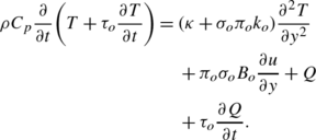  (18)

Let us introduce the following non-dimensional variables:

$$ \everymath{\displaystyle} \begin{array}{l} y^{*} = \frac{ U}{\upsilon} y ,\qquad t^{*} = \frac{ U^{2}}{\upsilon} t ,\qquad \tau_{o}^{*} = \frac{ U^{2}}{\upsilon} \tau_{o},\\[9pt] u^{*} = \frac{u}{U}, \qquad \varTheta = \frac{T - T_{\infty }}{T_{o}},\\[9pt] Q^{*} = \frac{\upsilon^{2} Q}{\kappa U^{2} T_{o}}, \qquad q^{*} = \frac{\upsilon}{\kappa T_{o} U} q,\\[9pt] P_{r} = \frac{C_{p}\mu}{\kappa} ,\qquad K_{o} = \frac{k_{o}\sigma_{o}B_{o}T_{o}}{\rho U^{2}},\\[9pt] \varPi_{o} = \frac{\pi_{o}\upsilon \sigma_{o}B_{o}}{\kappa T_{o}},\qquad M = \frac{\upsilon \sigma_{o}B_{o}^{2}}{\rho U^{2}}. \end{array} $$

(19)

Equations (17) and (18) are reduce to the nondimensional equations

(20)

(21)

We will also assume that the initial state of the medium is quiescent. Taking Laplace transform, defined by the relation

$$\bar{g}(s) = \int_{0}^{\infty } e^{ - st}g(t) dt, $$

of both sides of Eqs. (20) and (21), we obtain

(22)

(23)

where

We shall choose as state variables the temperature increment Θ, the velocity component in x-direction is u and their gradients. Equations (22) and (23), which can be written in the matrix form as

$$ \frac{{d}\bar{\boldsymbol{G}}{ (y,s)}}{{dy}}= \boldsymbol{A}(s) \boldsymbol{G}(y,s) + \boldsymbol{B}(y,s) , $$

(24)

where

The formal solution of Eq. (24) can be expressed as

(25)

In the special case when there is no heat source acting inside the medium, Eq. (25) simplifies to

$$ \bar{\boldsymbol{G}}(y,s) = \exp \bigl[ \boldsymbol{A}(y,s) y \bigr]\bar{\boldsymbol{G}}(0,s). $$

(26)

The characteristic equation of the matrix A(s) is

$$ k^{4} - (a + c - K_{o}d) k^{2} + ac = 0 , $$

(27)

where k is a characteristic root. The Cayley-Hamilton theorem states that the matrix A satisfies its own characteristic equation in the matrix sense. Therefore, it follows that

$$ \boldsymbol{A}^{{4}} - (a + c - K_{o}d) \boldsymbol{A}^{{2}} + a c \boldsymbol{I} = 0 . $$

(28)

Equation (28) shows that A ⁴ and all higher powers of A can be expressed in terms of A ³, A ², A and I, the unit matrix of order 4. The matrix exponential can now be written in the form

(29)

The scalar coefficients of Eq. (28) are now evaluated by replacing the matrix A by its characteristic roots ±k ₁ and ±k ₂, which are the roots of the biquadratic equation (27), satisfying the relations

(30a)

(30b)

This leads to the system of equations

(31a)

(31b)

The general solution of the above system is given by

(32)

Substituting the expression (32) into Eqs. (31a), (31b) and computing A ², and A ³, we obtain after some lengthy algebraic manipulations,

(33)

where the elements l _ij (y,s) are given by

(34)

It is worth mentioning here that Eqs. (30a) and (30b) have been used repeatedly in order to write the above entries in the simplest possible form. Furthermore, it should be noted that the corresponding expressions for generalized magneto-thermo viscous fluid with relaxation time in the absence of thermoelectricity effects can be deduced by setting ZT _o =K _o =Π _o =0 in Eq. (34).

It is now possible to solve a broad class of one-dimensional problems of generalized magneto-thermo viscous fluid flow with thermoelectric properties.

4 Applications

4.1 Problem I. A thermal shock semi-space problem

We consider a semi-space homogeneous viscoelastic conducting medium occupying the region y≥0 with quiescent initial state. A thermal shock is applied to the boundary plane y=0 in the form

$$ \theta( 0 , t ) = \theta_{o} H(t), $$

(35)

where, θ _o is a constant and H(t) is the Heaviside unit step function and the boundary plane y=0 is taken to be a fixed plane, i.e.

$$ u ( 0,t ) = 0. $$

(36)

Since the solution is unbounded at infinity, the initial conditions should be so adjusted that the infinite terms are eliminated.

We now apply the state space approach described above to this problem. The two components of the transformed initial state (0,s) are known, namely,

$$ \bar{\theta} ( 0,s ) = \frac{\theta_{o}}{s}, $$

(37)

which follows from (35) and

$$ \bar{u} ( 0,s ) = 0, $$

(38)

which follows from (36).

To obtain the two remaining components $\bar{u}'(0,s)$ and $\bar{\theta'} ( {0,s} )$, we substitute y=0 in both sides of (25) and in performing the necessary matrix operations, we obtain a system of linear algebraic equations in the two unknowns $\bar{u}'(0,s)$ and ${\bar{\theta'}} ( {0,s} )$, whose solution gives

(39)

(40)

Inserting the values from (37)–(40) into the right-hand side of (25), we obtain upon using (30a), (30b)

(41)

(42)

In non-dimensional form, the expression for the skin-friction component τ in the main flow is:

$$ \bar{\tau} = \biggl( \frac{\partial \bar{u}}{\partial y} \biggr)_{y = 0} = \frac{K_{o} c \theta_{o}}{s(k_{1}k_{2} + c)} . $$

(43)

4.2 Problem II. A problem of a layer media

We consider, now, a conducting viscoelastic fluid occupying the region 0≤y≤Y bounded by two parallel walls in the presence of a transverse magnetic field applied externally. Initially both the plates and fluid are assumed to be at rest. Let us suddenly impart a constant velocity U to the lower plate in its own plane in the presence of magnetic field.

The mechanical boundary conditions can be written as

(44)

(45)

The thermal boundary conditions are assumed to be

(46)

(47)

Condition (46) means that the plate y=0, is acted on by a constant thermal shock at time t=0, while condition (47) signifies that the plate y=Y, is thermally insulated.

Equations (43) and (46) give two components of the initial state vector $\bar{G}(0, s)$. To obtain the remaining two components, we use (26) between y=0 and y=Y to obtain the following two simultaneous linear equations:

The solution of these equations gives

(48)

(49)

Inserting the values from Eqs. (44)–(49) into the right-hand side of Eq. (26), we obtain upon using Eqs. (30a), (30b)

(50)

(51)

4.3 Problem III. Plane distribution of heat sources

We assume that there is a plane distribution of continuous heat sources located at the plate y=0. The intensity of the heat sources is thus given by

$$Q(y,t) = Q_{o} H(t) \delta(y), $$

where Q _o is a constant and δ(y) is Dirac’s delta function. Taking Laplace transform, we obtain

$$ \bar{Q}(y,s) = Q_{o}\frac{\delta (y)}{s}. $$

(52)

We shall now proceed to obtain the solution of the problem for the region y≥0. The solution for the other region is obtained by replacing each y by −y.

Evaluating the integral in Eq. (25) using the integral properties of the Dirac delta function, we obtain

$$ \bar{\boldsymbol{G}}(y,s) = \boldsymbol{L}(y,s) \bigl[\bar{\boldsymbol{G}}(0,s) + \boldsymbol{H}(s)\bigr], $$

(53)

where

$$\boldsymbol{B}(y,s) = - \frac{Q_{o}\beta}{4s} \left[ \begin{array}{l} \frac{k_{1}k_{2} + a}{k_{1} + k_{2}} \\ 0 \\ 1 \\ \frac{K_{o}}{k_{1} + k_{2}} \end{array} \right]. $$

Equation (53) expresses the solution of the problem in the Laplace transform domain in terms of the vector H(s) representing the applied heat source and the vector $\bar{\boldsymbol{G}}(0,s)$ representing the conditions at the plane source of heat. In order to evaluate the components of this vector, we note first that due to the symmetry of the problem, the temperature is a symmetric of y while the velocity is anti-symmetric. It thus follows that

$$ u ( 0,t ) = 0\quad \mbox{or}\quad\bar{u} ( 0,s ) = 0. $$

(54)

Gauss’s divergence theorem will now be used to obtain the thermal condition at the plane source. We consider a short cylinder of unit base whose axis is perpendicular to the plane source of heat and whose bases lie on opposite sides of it. Taking limits as the height of the cylinder tends to zero and noting that there is no heat flux through the lateral surface, upon using the symmetry of the temperature field we get

$$ q (0,t) = \frac{Q_{o}}{2} H(t) \quad\mbox{or}\quad\bar{q}(0,s) = \frac{Q_{o}}{2s}. $$

(55)

Using Fourier’s law of heat conduction in the non-dimensional form, namely

$$ q = - \frac{1 + ZT_{o}}{1 + \tau_{o}s} \varTheta' - \frac{\varPi_{o}}{1 + \tau_{o}s} u, $$

(56)

we obtain the condition

$$ \varTheta'(0,s) = - \frac{\beta Q_{o}}{2s} . $$

(57)

Equations (54) and (57) give two components of the vector $\bar{\boldsymbol{G}}(0,s)$. In order to obtain the remaining two components, we substitute y=0 on both sides of Eq. (53) obtaining a system of linear equations whose solution gives

(58)

(59)

As before, we have suppressed the positive exponential terms appearing in the entries of L(y,s). Substituting the above values in the right-hand side of Eq. (53), we obtain

(60)

(61)

In the above equations the upper (plus) sign indicates the solution in the region y<0, while the lower (minus) sign indicates the region y≥0, respectively.

5 Numerical inversion of the Laplace transforms

In order to invert the Laplace transform in the above equations, we adopt a numerical inversion method based on a Fourier series expansion [32]. In this method, the inverse g(t) of the Laplace transform $\bar{g}(s)$ is approximated by the relation

(62)

where c ^∗ is an arbitrary constant greater than all the real parts of the singularities of g(t) and N is sufficiently large integer chosen such that,

$$ e^{c^* t}\operatorname{Re}\biggl[ \exp\biggl( \frac{i N \pi t}{t_{1}} \biggr) \bar{g} \biggl(c* + \frac{i N \pi}{ t_{1}} \biggr) \biggr] \le \varepsilon, $$

(63)

where ε is a prescribed small positive number that corresponds to the degree of accuracy required.

Using the numerical procedure cited, to invert the expressions of temperature, velocity and microrotation, fields in Laplace transform domain.

6 Results and discussions

The investigation of the effect of the magnetic field parameter M and the thermoelectric coefficients are named for Seebeck coefficient K _o and Peltier coefficient Π _o as well as the efficiency of a thermoelectric material figure-of-merit ZT _o on the flow of viscous fluid over the boundaries, in the presence of magnetic field has been carried out in the preceding sections. This enables us to represent the typical numerical results in Figs. 1–9, for the temperature θ and velocity component u for various values of the parameters. Hence we conclude with following points:

• (i) The important phenomenon observed in all computations is that the solution of any of the considered functions vanishes identically outside a bounded region of space surrounding the heat source at a distance from it equal to y ^∗(t); say y ^∗(t) is a particular value of y depending only on the choice of t and is the location of the wave front. This demonstrates clearly the difference between the solution corresponding to using classical Fourier heat equation (τ ₀=0.0) and to using the generalized Fourier case (τ ₀=0.2). In the first and older theory the waves propagate with infinite speeds, so the value of any of the functions is not identically zero (though it may be very small) for any large value of y. In non-Fourier theory the response to the thermal and mechanical effects does not reach infinity instantaneously but remains in a bounded region of space given by 0<y<y ^∗(t) for the semi space problem.

• (ii) The Seebeck and Peltier effects are shown to be closely related within the new thermodynamic model applied recently to the quantitative theory of the Seebeck coefficient. In this work, the model was developed for the evaluation of the Seebeck and Peltier coefficients. The gradual decrease of temperature with as shown in Fig. 1 has also been reported by Huston [43], Ambia et al. [44] and Patankar et al. [45]. In Fig. 2 we observe that the Peltier coefficient is proportional to the temperature at constant value of Seebeck coefficient. These results agrees with the expectation by the first Thomson relation Π=ST [14].

  Fig. 1

  

  A plot of the temperature as a function of the Seebeck coefficient for different values of Peltier coefficient in Problem I

  Fig. 2

  

  A plot of the temperature as a function of the Peltier coefficient for different values of thermoelectric figure-of-merit in Problem I

• (iii) Figure 3 presents some data on the temperature as a function of figure-of- merit of various thermoelectric fluids [46, 47].

  Fig. 3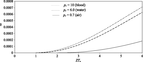

  

  A plot of the temperature as a function of the figure-of-merit for several thermoelectric fluids in Problem I

• (iv) In Fig. 4, we observe that when ZT _o =1, the velocity waves cut the y-axis rapidly when ZT _o >1.

  Fig. 4

  

  A plot of the velocity for different values of thermoelectric figure-of-merit in Problem I

• (v) Figures 5 and 6 give the spatial variation of temperature and velocity for different values of the thermoelectric figure-of-merit ZT _o , and the magnetic parameter M. From these figures we learn that the temperature increases with the increase in the value of thermoelectric figure-of-merit. The magnetic number acts to decrease in the velocity component of the fluid and it thus turns out that under the action of a magnetic field, in an electrically conducting fluid (e.g. blood), there develops a resistive force (Lorentz force) which causes impedance of flow.

  Fig. 5

  

  A plot of the temperature for different values of thermoelectric figure-of-merit in Problem II

  Fig. 6

  

  A plot of the velocity for different values of magnetic parameter in Problem II

• (vi) The temperature and velocity distributions for a problem for the infinite space in the presence of heat sources are represented graphically in Fig. 7 and for different values of figure-of-merit ZT _o . We notice that the efficiency of a thermoelectric material figure-of-merit is proportional to the temperature and the velocity of the fluid particles as shown in Fig. 8.

  Fig. 7

  

  A plot of the temperature for different values of thermoelectric figure-of-merit in Problem III

  Fig. 8

  

  A plot of the heat flux for different values of thermoelectric figure-of-merit in Problem III

• (vii) Investigation of heat transfer, in particular, free-convection heat transfer, involves measuring a heat flux on a surface along which a liquid moves [48]. The non-dimensional Fourier heat conduction in terms of thermoelectric figure-of-merit and Peltier coefficient. In Fig. 9, we observe that the effect of thermoelectric figure-of-merit on the heat flux distribution over the plane surface. It is notice that heat flux increases with increasing figure-of merit in the boundary layer region [49].

  Fig. 9

  

  A plot of the heat flux for several thermoelectric fluids with different values of thermoelectric figure-of-merit in Problem III

• (viii) The method used in the present work is applicable to a wide range of problems. It can be applied to problems that are described by linear-system equations [50–52]. The same approach was used quite successfully in dealing with problems in thermoelasticity theory [53–58].

7 Conclusions

The main goal of this work is to introduce a new mathematical model for the boundary layer flow of viscous thermofluids over the boundaries in the presence of magnetic field. This model is to analyse in some detail the influence of thermoelectric properties on that flow. The effects of figure-of-merit, Seebeck and Peltier coefficients on the flow of electro conducting viscous fluids over boundaries in the presence of magnetic field are presented. The result provides a motivation to investigate conducting thermofluids as a new class of applicable thermoelectric materials.

References

Ezzat MA (2008) State space approach to solids and fluids. Can J Phys Rev 86:1242–1450
Borghesani R, Morro A (1974) The thermodynamic restrictions on thermoelectric, thermomagnetic galvanomagnetic coefficients. Meccanica 9:157–161
Nolas GS, Johnson D, Mandrus DG (2002) Thermoelectric materials and devices. Materials Research Society, Warrendale, p 691
Rowe DM (1995) CRC handbook of thermoelectrics. CRC Press, Boca Raton
Ezzat MA (2010) Thermoelectric MHD non-Newtonian fluid with fractional derivative heat transfer. Physica B 405:4188–4194
Raffa FA, Roccato PE, Zucca M (2011) Realization of a new experimental setup for magnetostrictive actuators. Meccanica 46:979–987
La Bounty C, Shakouri A, Bowers GE (2001) Design and characterization of thin film microcoolers. J Appl Phys 89:4059–4064
Mahan G, Sales B, Sharp J (1997) Thermoelectric materials: new approaches to an old problem. Phys Today 50:42–47
Mahtur RG, Mehra RM (1998) Thermoelectric power in porous silicon. J Appl Phys 83:5855–5857
Menčík J (2007) Determination of mechanical properties by instrumented indentation. Meccanica 42:19–29
Hicks LD, Dresselhaus MS (1993) Thermoelectric figure of merit of a one-dimensional conductor. Phys Rev B 47:16631–16634
Venkatasubramanian R, Silvola E, Colpitts T, O’Quinn B (2001) Thin-film thermoelectric devices with high room-temperature figures of merit. Nature 413:597
Zhou J, Balandin A (2001) Phonon heat conduction in a semiconductor nanowire. J Appl Phys 89:2932–2938
Morelli DT (1997) Thermoelectric devices. In: Trigg GL, Immergut EH (eds) Encyclopedia of applied physics, vol 21. Wiley-VCH, New York, pp 339–354
Schlichting H, Gersten K (2000) Boundary layer theory, 8th edn. Springer, Berlin
Tanner R (1962) Notes on the Rayleigh parallel problem for a viscoelastic fluid. Z Angew Math Phys 13:573–580
Preziosi L, Joseph D (1987) Stokes first problem for viscoelastic fluids. J Non-Newton Fluid Mech 25:239–259
Phan-Thien N, Chew YT (1988) On the Rayleigh problem for a viscoelastic fluid. J Non-Newton Fluid Mech 28:117–127
Nadeem S, Asghar S, Hayat T, Hussain M (2008) The Rayleigh Stokes problem for rectangular pipe in Maxwell and second grade fluid. Meccanica 43:495–504
Singh J, Glière A, Jean-Luc A (2012) A novel non-primitive boundary integral equation method for three dimensional and axisymmetric Stokes flows. Meccanica 47:1–14
Joneidi A, Domairry G, Babaelahi M (2010) Homotopy analysis method to Walter’s B fluid in a vertical channel with porous wall. Meccanica 45:857–868
Yadav PK, Deo S (2012) Stokes flow past a porous spheroid embedded in another porous medium. Meccanica 47:1499–1516
Fetecau C, Sharat C, Rajagopal K (2007) A note on the flow induced by a constantly accelerated plate in an Oldroyd-B fluid. Appl Math Model 31:647
Abel MS, Tawade JV, Nandeppanavar MM (2012) MHD flow and heat transfer for the upper-convected Maxwell fluid over a stretching sheet. Meccanica 47:385–393
Andersson HI (1992) MHD flow of a viscoelastic fluid past a stretching surface. Acta Mech 95:227–230
Mahmoud MA, Megahed AM (2012) Non-uniform heat generation effect on heat transfer of a non-Newtonian power-law fluid over a non-linearly stretching sheet. Meccanica 47:1131–1139
Sakiadis BC (1961) Boundary layer behavior on continuous solid surfaces: I Boundary layer equations for two dimensional and axisymmetric flow. AIChE J 7:26–28
Ezzat MA, Othman MI, Helmy KA (1999) A problem of a micropolar magnetohydrodynamic boundary-layer flow. Can J Phys 77:813–827
Othman MI, Ezzat MA (2001) Electromagneto-hydrodynamic instability in a horizontal viscoelastic fluid layer with one relaxation time. Acta Mech 150:1–9
Ezzat MA (2001) Free convection effects on perfectly conducting fluid. Int J Eng Sci 39:799–819
Walters K (1958) Viscoelasticity and rheology, vol 20. Academic Press, New York, pp 47–79
Honig G, Hirdes U (1984) A method for the numerical inversion of the Laplace transform. J Comput Appl Math 10:113–132
Cattaneo C (1948) Sullacodizion del calore. Atti Semin Mat Fis Univ Modena 3:83–101
Truesdell C, Muncaster RG (1980) Fundamentals of Maxwell’s kinetic theory of a simple monatomic gas. Academic Press, New York
Lebon G, Rubi JM (1980) A generalized theory of thermoviscous fluids. J Non-Equilib Thermodyn 5:285–300
Ezzat MA (2012) State space approach to thermoelectric fluid with fractional order heat transfer. Heat Mass Transf 48:71–82
Joseph DD, Preziosi L (1989) Heat waves. Rev Mod Phys 61:41–73
Ezzat MA, Youssef HM (2012) Stokes’ first problem for an electro-conducting micropolar fluid with thermoelectric properties. Can J Phys 88:35–48
Shercliff JA (1979) Thermoelectric magnetohydrodynamics. J Fluid Mech 191:231–251
Villaggio P (2011) Sixty years of solid mechanics. Meccanica 46:1171–1189
Ceniga L (2012) Thermal stress induced phenomena in two-component material: Part II. Meccanica 26:101–106
Ishak A, Yacob NA, Bachok N (2011) Radiation effects on the thermal boundary layer flow over a moving plate with convective boundary condition. Meccanica 46:795–801
Hutson AR (1959) Electronic properties of ZnO. J Phys Chem Solids 8:467–472
Ambia MG, Islam MN, Hakim MO (1992) Studies on the Seebeck effect in semiconducting ZnO thin films. J Mater Sci 27:5169–5173
Patankar KK, Mathe VL, Patil AN, Patil SA, Lotke SD (2001) Electrical conduction and magnetoelectric effect in CuFe1.8Cr0.2O4–Ba0.8Pb0.2TiO3 composites. J Electroceram 6:115–122
Tritt TM (2000) Semiconductors and semimetals, recent trends in thermoelectric materials research, vols 69–71. Academic Press, San Diego
Nolas GS, Sharp J, Goldsmid HJ (2001) Thermoelectrics: basic principles and new materials developments. Springer, New York
Mityakov AV, Mityakov YV, Sapozhnikov SZ, Chuma YS (2002) Methods of experimental investigation and measurement: application of the transverse Seebeck effect to measurement of instantaneous values of a heat flux on a vertical heated surface under conditions of free-convection heat transfer. High Temp 40:620
Phani KM, Gopinath RW, Vijay KD (2009) Wall heat flux partitioning during subcooled forced flow film boiling of water on a vertical surface. Int J Heat Mass Transf 52:3534–3546
Ezzat MA, El-Bary A, Ezzat SM (2011) Combined heat and mass transfer for unsteady MHD flow of perfect conducting micropolar fluid with thermal relaxation. Energy Convers Manag 52:934–945
Devakar M, Lyenger TK (2009) Stokes’ first problem for a micropolar fluid through state-space approach. Appl Math Model 33:924–936
Ezzat MA, Abd-Elaal MZ (1997) State space approach to viscoelastic fluid flow of Hydromagnetic fluctuating boundary-layer through a porous medium. Z Angew Math Mech 77:197–207
Ezzat MA, Othman MI, Smaan AA (2001) State space approach to two-dimensional electromagneto-thermoelastic problem with two relaxation times. Int J Eng Sci 39:1383–1404
Ezzat MA, El-Karamany AS (2003) Magnetothermoelasticity with two relaxation times in conducting medium with variable electrical and thermal conductivity. Appl Math Comput 142:449–467
Ezzat MA (2006) The relaxation effects of the volume properties of electrically conducting viscoelastic material. Mater Sci Eng B 130:11–23
Ezzat MA, El-Bary AA (2009) State space approach of two-temperature magneto-thermoelasticity with thermal relaxation in a medium of perfect conductivity. Int J Eng Sci 47:618–630
Ezzat MA (2011) Magneto-thermoelasticity with thermoelectric properties and fractional derivative heat transfer. Physica B 406:30–35
Ezzat MA, El-Karamany AS (2011) Two-temperature theory in generalized magneto-thermoelasticity with two relaxation times. Meccanica 46:785–794
Author information
Authors and Affiliations
Corresponding author
Rights and permissions
About this article
Cite this article
Ezzat, M.A., El-Bary, A.A. & Ezzat, S.M. Stokes’ first problem for a thermoelectric Newtonian fluid. Meccanica 48, 1161–1175 (2013). https://doi.org/10.1007/s11012-012-9658-7
Received:
Accepted:
Published:
Issue Date:
DOI: https://doi.org/10.1007/s11012-012-9658-7