
Abstract
The q-rung orthopair fuzzy sets dynamically change the range of indication of decision knowledge by adjusting a parameter q from decision makers, where \(q \ge 1\), and outperform the conventional intuitionistic fuzzy sets and Pythagorean fuzzy sets. Linguistic q-rung orthopair fuzzy sets (Lq-ROFSs), a qualitative type of q-rung orthopair fuzzy sets, are characterized by a degree of linguistic membership and a degree of linguistic non-membership to reflect the qualitative preferred and non-preferred judgments of decision makers. Einstein operator is a powerful alternative to the algebraic operators and has flexible nature with its operational laws and fuzzy graphs perform well when expressing correlations between attributes via edges between vertices in fuzzy information systems, which makes it possible for addressing correlational multi-attribute decision-making (MADM) problems. Inspired by the idea of Lq-ROFS and taking the advantage of the flexible nature of Einstein operator, in this paper, we aim to introduce a new class of fuzzy graphs, namely, linguistic q-rung orthopair fuzzy graphs (Lq-ROFGs) and further explore efficient approaches to complicated MAGDM situations. Following the above motivation, we propose the new concepts, including product-connectivity energy, generalized product-connectivity energy, Laplacian energy and signless Laplacian energy and discuss several of its desirable properties in the background of Lq-ROFGs based on Einstein operator. Moreover, product-connectivity energy, generalized product-connectivity energy, Laplacian energy and signless Laplacian energy of linguistic q-rung orthopair fuzzy digraphs (Lq-ROFDGs) are presented. In addition, we present a graph-based MAGDM approach with linguistic q-rung orthopair fuzzy information based on Einstein operator. Finally, an illustrative example related to the selection of mobile payment platform is given to show the validity of the proposed decision-making method. For the sake of the novelty of the proposed approach, comparison analysis is conducted and superiorities in contrast with other methodologies are illustrated.
1 Introduction
With the advent of the era of big data, practical problems and actual scenarios in real life have become more complicated. In some cases, Pythagorean fuzzy set (PFS) (Yager and Abbasov 2013) and intuitionistic fuzzy set (IFS) (Atanassov 1986) cannot effectively deal with certain types of data. To solve this issue, Yager (2016) put forward the concept of q-rung orthopair fuzzy sets (q-ROFSs), which generalize the classical IFSs and PFSs. q-ROFSs provide more freedom and choice for decision makers by allowing the sum of the \(q^{th}\) power of the membership degree (MD) and the \(q^{th}\) power of the non-membership degree (NMD) to be less than or equal to 1. The above information can be illustrated as \(Q=(0.6, 0.9)\); it is q-rung orthopair fuzzy number, but not an intuitionistic fuzzy number and Pythagorean fuzzy number (because \(0.6^{q}+ 0.9^{q} \le 1\) and \(0.6^{2}+ 0.9^{2} >1\), \(0.6+ 0.9 >1\) ). The q-ROFSs reduced to IFSs, PFSs and Fermatean fuzzy sets (Senapati and Yager 2020) when \(q=1\), \(q=2\) and \(q=3\), respectively. When q expands, the q-ROFSs give more freedom to decision makers to provide their assessment data. Recently, many researchers developed several decision-making methods under generalized fuzzy scenario (Akram et al. 2020; Akram and Shahzadi 2020; Akram et al. 2021, 2020; Feng et al. 2021; Abdullah and Aslam 2020; Ashraf et al. 2019a, b, c; Liu et al. 2021; Qiyas et al. 2020; Zhan et al. 2018; Zhang and Li 2019).
For certain qualitative attributes, in some complicated decision-making problems, the decision makers cannot assign the MD and NMD by crisp numbers, and a feasible solution is to describe them by linguistic variables (LVs). Lin et al. (2020) developed Lq-ROFSs and devised the operational laws, such as weighted averaging operator and weighted geometric operator based on Lq-ROF environment to aggregate the Lq-ROF numbers. Obviously, Lq-ROFS can be regarded as the extension of the linguistic intuitionistic fuzzy set (LIFS) (Zhang 2014) and linguistic Pythagorean fuzzy set (LPFS) (Garg 2018; Lin et al. 2018), when \(q = 1\) and \(q=2\) the Lq-ROFS reduces to LIFS and LPFS, respectively. Wang et al. (2019) introduced some basic concepts of Lq-ROFS and developed some new operational laws, comparison methods, and distance measure methods with Lq-ROFS. Liu et al. (2019) proposed a new class of fuzzy sets (Zadeh 1965) called q-rung orthopair uncertain linguistic sets based on the q-ROFSs and uncertain linguistic variables and developed uncertain linguistic aggregation operators. Yue et al. (2020) put forward several new operational laws of probabilistic linguistic term sets along with its application in MADM. Amin et al. (2020) developed MADM approach on the basis of triangular cubic linguistic uncertain fuzzy aggregation operators. Table 1 expresses the superiority and flexibility of the Lq-ROFS model compared to some of the existing models in literature.
Graphs can be used to model many real life systems. The graphs demonstrate the connections within these systems between the entities. As in electrical networks and computer networks, the connections may be physical or relationships as in molecules and ecosystems. Graphs are abstractions of these connections. The spectrum is the set of all eigenvalues of a graph. There has been detailed analysis of spectral properties of graphs. Gutman (2001) proposed the concept of the graph energy in chemistry and evaluated lower and upper limits for the energy of the graph. If a graph is connected, its distance and adjacent energy is computed as the sum of the absolute values of the associated eigenvalues. If graph is not connected, then a graph’s energy is the sum of the energy of its connected components. The Laplacian matrix L(G) of a graph G is obtained by subtracting the adjacency matrix A(G) from its degree matrix D(G) whose vertex \(f_{i}\) has degree \(d_{i}\) is defined by \(d_{G}(r_{i})\) when \(i=j\) and 0 otherwise. Signless Laplacian matrix \(L^{+}(G)\) of a graph G is obtained by adding the adjacency matrix A(G) in its degree matrix D(G). Laplacian energy (Gutman and Zhou 2006) and signless Laplacian energy (Gutman et al. 2010) of a graph is the sum of the absolute values of the differences of the average vertex degree of G to the Laplacian and signless Laplacian eigenvalues of G, respectively. Graphs are representations of binary relations. Similarly, fuzzy binary relations are represented by graphs called fuzzy graphs (FGs). Fuzzy graphs are generalizations of crisp graphs. Rosenfeld (1975) suggested the idea of FGs and established its structure. Anjali and Mathew (2013) evaluated the energy of FGs.
Naz et al. originally introduced some new classes of FGs called PFGs (Naz et al. 2018) and complex PFGs (Akram and Naz 2019) along its pertinent applications in decision making. Akram and Naz (2018) discussed the theory of graph spectra in the context of the generalized fuzzy circumstances which deal MADM information more objectively. A new concept of q-rung orthopair fuzzy graphs was put forward by Habib et al. (2019) along its application in the soil ecosystem.
Koczy et al. (2020) put forward the notion of picture fuzzy graphs and analyze a Wi-Fi network and a social network based on picture fuzzy graphs. Akram et al. (2021) and Akram and Luqman (2020) defined trapezoidal picture fuzzy numbers along with its graphical representation and proposed a new approach of formation of granular structures based on fuzzy soft graphs. Recently, novel concepts of Zagreb and Harmonic energy in the background of interval-valued q-rung orthopair dual hesitant fuzzy Hamacher graphs are incorporated by Naz et al. (2021). Apart from this, some novel concepts of energy based on well-known molecular descriptors geometric-arithmetic and the atom bond connectivity of dual hesitant q-ROFGs have been presented by Akram et al. (2021).
Einstein operator not only a good alternative to the algebraic operator, and gives the same smooth approximations as the algebraic but also has more and more flexibility and robustness than algebraic operator. Due to the uncertainty of information data from some practical decision-making problems with the interrelated criteria, it might be tough for the decision makers to precisely quantify their judgment with a classical number, but can represent them by natural language. Lq-ROFS theory is one of the successful generalizations of linguistic fuzzy set theory which provides greater range for decision makers to express their uncertain, vague and imprecise information in natural language, and graphs play an essential role in modern world, due to its broadly spread use for representing, modeling and organizing linked data. In this manner, it is very significant to present the idea of Lq-ROFGs that not only accommodates Lq-ROF information but also can capture the relationships among arguments. To achieve this goal, utilizing LFSs into q-ROFGs, we introduce a new class of fuzzy graphs called linguistic q-rung orthopair fuzzy graphs (Lq-ROFGs) on the basis of Einstein operator and discuss its spectra. Due to its simple analysis and computational flexibility, the presented study has a distinct advantage over the others. The main contributions of this research are:
-
(1)
to incorporate the theory of LFSs into q-ROFGs and propose a new, powerful tool for describing interrelated uncertain phenomena, called Lq-ROFGs based on Einstein operator;
-
(2)
to propose the new concepts of the product-connectivity energy, generalized product-connectivity energy, Laplacian energy and signless Laplacian energy of Lq-ROFGs, as well as the Lq-ROFDGs;
-
(3)
to develop a MAGDM method based on Lq-ROFG and Einstein operator;
-
(4)
to solve decision-making problem related to mobile payment platform selection to illustrate the applicability and effectiveness of our proposed approach.
Compared with many existing generalized fuzzy graph theories, the newly proposed Lq-ROFGs show extraordinary flexibility and effectiveness and can successfully express the decision-making opinions of decision experts. The most beneficial advantage of the Lq-ROFG is that it uses linguistic terminology to describe the qualitative evaluation details provided by decision makers for a specific evaluation object.
Remaining paper is organized as follows: Sect. 2 recalls some basic definitions related to this paper. Section 3 introduces the concept of Lq-ROFG based on Einstein operator, the spectra of a graph in Lq-ROF environment and briefly discusses its certain properties. Section 4 find out the product-connectivity energy, generalized product-connectivity energy, Laplacian energy, and signless Laplacian energy of Lq-ROFDGs based on Einstein operator. In Sect. 5, a graph-based MAGDM approach with Lq-ROF information is given and illustrative example shows the validity of our proposed method. Finally, we summarize the paper in Sect. 6.
2 Preliminaries
In this section, the basic concepts of LTS and Lq-ROFS are provided to facilitate the next sections.
Definition 1
(Dutta and Guha 2015) Let there exist a finite LTS \(S=\{{s}_{\gamma }|\gamma =0, 1,\ldots , \tau \}\) with odd cardinality, where \({s}_{\gamma }\) indicates a possible linguistic term. For instance, a LTS S having seven terms can be described as follows:
Generally, the LTS meets the following characteristics:
-
(i)
The set is ordered: \({s}_{k}>{s}_{l}\), if and only if \(k>l.\)
-
(ii)
Max operator: \(\max ({s}_{k}, {s}_{l})={s}_{k},\) if and only if \(k\ge l\).
-
(iii)
Min operator: \(\min ({s}_{k}, {s}_{l})={s}_{k},\) if and only if \(k\le l\).
-
(iv)
Negative operator: Neg\(({s}_{k})={s}_{l}\) such that \(l=\tau -k.\)
Definition 2
(Lin et al. 2020) If there is a finite reference set \(U=\{r_{1}, r_{2},\ldots , r_{n}\}\) and a continuous LTS (CLTS) \(S=\{{s}_{\gamma }|\gamma \in [0, \tau ]\}\) with a nonnegative integer \(\tau \); then Lq-ROFS on U is expressed as
characterized as the membership function \({s}_{a}(r)\) and non-membership function \({s}_{b}(r)\) of an element r. Each orthopair \(({s}_{a}(r), {s}_{b}(r))\) in the Lq-ROFS \({\mathcal {L}}\) is considered as a Lq-ROFN and is simplified as \(({s}_{a}, {s}_{b})\). In each orthopair \(({s}_{a}, {s}_{b})\), \({s}_{a}\) and \({s}_{b}\) must fulfill the condition: \(a, b \in [0, \tau ]\) and \(0\le a^{q} + b^{q} \le \tau ^{q}\) with \(q\ge 1\). Further, \({s}_{\pi }(r) = {s}_{\root q \of {\tau ^{q}-a^{q}-b^{q}}}\) is the hesitant degree of the element r.
Definition 3
(Lin et al. 2020) Consider a Lq-ROFN \(p=({s}_{a}, {s}_{b})\) with \({s}_{a}, {s}_{b} \in S\) and a CLTS \(S=\{{s}_{\gamma }|\gamma \in [0, \tau ]\}\), then the score value of the Lq-ROFN is described as
and its accuracy value is described as
Any two Lq-ROFNs \(p_{1}\) and \(p_{2}\) are compared by the following developed method as follows:
-
(1)
if \({\mathcal {S}}(p_{1})>{\mathcal {S}}(p_{2}),\) then \(p_{1}\succ p_{2};\)
-
(2)
if \({\mathcal {S}}(p_{1})={\mathcal {S}}(p_{2}),\) then: (a) if \(J(p_{1})>J(p_{2}),\) then \(p_{1}\succ p_{2}\); (b) if \(J(p_{1})=J(p_{2}),\) then \(p_{1}\sim p_{2}.\)
To illustrate the difference among linguistic intuitionistic fuzzy numbers (LIFNs), linguistic Pythagorean fuzzy numbers (LPFNs) and linguistic q-rung orthopair fuzzy numbers (Lq-ROFNs), we present their space of acceptable membership degrees in Figs. 1, 2 and 3.

The distribution area of LIFNs in a LIFS

The distribution areas for LIFNs and LPFNs

The distribution areas for Lq-ROFNs
Figures 1, 2 and 3 clearly show that as the index of \(s_a\) and \({s}_{b}\) increases, so does the range of information which can be described by the fuzzy numbers. The Lq-ROFNs can therefore enlarge the information which the attributes can portray and expand the space for decision makers to evaluate alternatives. It can also be observed that each of LIFS and LPFS is also a Lq-ROFS with \(q \ge 1\) and \(q \ge 2\), respectively.
Definition 4
(Wang and Liu 2011) For any two real numbers \(r,s\in [0, 1]\), the Einstein t-norm and t-conorm are defined as follows:
Some notations used in this paper are listed in Table 2.
3 Linguistic q-rung orthopair fuzzy Einstein graphs
In this section, we introduce the innovative concept of Lq-ROFGs based on Einstein operator called Linguistic q-rung orthopair fuzzy Einstein graphs or simply Lq-ROFGs. Further, we discuss the spectra of a graph in Lq-ROF environment and discuss its certain properties.
Definition 5
Let U be the universe of discourse. A Lq-ROFS \({\mathcal {E}}\) in \(U\times U\) is said to be a linguistic q-rung orthopair fuzzy relation (Lq-ROFR) in U, denoted by
where \({s}_{{a}_{{\mathcal {E}}}}:U\times U \rightarrow [0, \tau ]\) and \({s}_{{b}_{{\mathcal {E}}}}:U\times U\rightarrow [0, \tau ]\) represent the membership and non-membership function of \({\mathcal {E}}\), respectively, such that \(0\le a_{{\mathcal {E}}}^{q}(rs)+ b_{{\mathcal {E}}}^{q}(rs)\le \tau ^{q}\) for all \(rs\in U\times U.\)
Definition 6
A Lq-ROFG based on Einstein operator under CLTS \(S=\{{s}_{\gamma }|\gamma \in [0, \tau ]\}\) with a positive integer \(\tau \) is a pair \({\mathcal {M}}=({\mathcal {L}}, {\mathcal {E}})\), where \({\mathcal {L}}\) is a Lq-ROFS on U and \({\mathcal {E}}\) is a Lq-ROFR on U such that:
and \(0\le a_{{\mathcal {E}}}^{q}(rs)+ b_{{\mathcal {E}}}^{q}(rs)\le \tau ^{q}\) for all \(r,s \in U.\) We call \({\mathcal {L}}\) and \({\mathcal {E}}\) the Lq-ROFS of vertices and the Lq-ROFS of edges of \({\mathcal {M}}\), respectively. Here, \({\mathcal {E}}\) is a symmetric linguistic q-rung orthopair fuzzy relation on \({\mathcal {L}}\). If \({\mathcal {E}}\) is not symmetric on \({\mathcal {L}}\), then \({\mathcal {D}}=({\mathcal {L}}, \mathcal {\overrightarrow{{\mathcal {E}}}})\) is called Lq-ROFDG.

Linguistic 3-rung orthopair fuzzy Einstein graph with CLTS \(S=\{{s}_{\gamma }|\gamma \in [0, 8]\}\)
The adjacency matrix \(A({\mathcal {M}})=(A({s}_{{a}_{{\mathcal {E}}}}(r_{i}r_{j})),A({s}_{{b}_{{\mathcal {E}}}}(r_{i}r_{j})))\) of a Lq-ROFG \({\mathcal {M}}=({\mathcal {L}},{\mathcal {E}})\) is a square matrix \(A({\mathcal {M}})=[a_{ij}],\) \(a_{ij}=({s}_{{a}_{{\mathcal {E}}}}(r_{i}r_{j}),{s}_{{b}_{{\mathcal {E}}}}(r_{i}r_{j}))\), where \({s}_{{a}_{{\mathcal {E}}}}(r_{i}r_{j})\) and \({s}_{{b}_{{\mathcal {E}}}}(r_{i}r_{j})\) indicate the relationship and non-relationship strength between \(r_{i}\) and \(r_{j}\), respectively.
Example 1
Consider a L3-ROFG \({\mathcal {M}}=({\mathcal {L}},{\mathcal {E}})\), shown in Fig. 4, which models collaboration between researchers. The researchers are represented by vertices \(V=\{f_{1}, f_{2}, f_{3},f_{4},f_{5},f_{6}\}\) and the collaborations between any two researchers are represented by edges \(E=\{f_{1}f_{2},f_{1}f_{4},f_{1}f_{5}\), \(f_{1}f_{6},f_{2}f_{3},f_{3}f_{4},f_{4}f_{5}\}\). Let \(S=\{{s}_{0}= \hbox {worst}\), \({s}_{1} = \hbox {very poor}\), \({s}_{2} = \hbox {poor}\), \({s}_{3} = \hbox {slightly poor}\), \({s}_{4}= \hbox {medium}\), \({s}_{5} = \hbox {slightly good}\), \({s}_{6} = \hbox {good}\), \(a_{7}= \hbox {very good}\), \({s}_{8}= \hbox {outstanding}\}\) be a CLTS. Then,
Clearly, \({\mathcal {M}}=({\mathcal {L}}, {\mathcal {E}})\) shown in Fig. 4, is a L3-ROFG. The adjacency matrix of the above Lq-ROFG \(A({\mathcal {M}})\) is as follows:
Now we put forward some new concepts of spectral graph theory including product-connectivity energy, generalized product-connectivity energy, Laplacian energy and signless Laplacian energy in Lq-ROF environment based on Einstein operator.
3.1 Generalized product-connectivity energy of Lq-ROFGs
This subsection defines and investigates the product-connectivity energy and generalized product-connectivity energy of a Lq-ROFG and provides its properties in detail.
Definition 7
Let \({\mathcal {M}}=({\mathcal {L}},{\mathcal {E}})\) be a Lq-ROFG on n vertices. The product-connectivity matrix, \(PC({\mathcal {M}})=(PC({s}_{{a}_{{\mathcal {E}}}}(r_{i}r_{j})), PC({s}_{{b}_{{\mathcal {E}}}}(r_{i}r_{j})))=[d_{ij}],\) of \({\mathcal {M}}\) is a \(n\times n\) matrix defined as:
Definition 8
The product-connectivity energy of a Lq-ROFG \({\mathcal {M}}=({\mathcal {L}},{\mathcal {E}})\) is defined as:
where \(N_{PC}\) and \(O_{PC}\) are the sets of product-connectivity eigenvalues of \(PC({{s}_{{a}_{{\mathcal {E}}}}}{(r_{i}r_{j})})\) and \(PC({{s}_{{b}_{{\mathcal {E}}}}}{(r_{i}r_{j})})\), respectively.
Now, we define generalized product-connectivity energy of the Lq-ROFG and provide its properties in detail.
Definition 9
Let \({\mathcal {M}}=({\mathcal {L}},{\mathcal {E}})\) be a Lq-ROFG on n vertices. The general product-connectivity matrix, \(PC_{\alpha }({\mathcal {M}})=(PC_{\alpha }({{s}_{{a}_{{\mathcal {E}}}}}{(r_{i}r_{j})}), (PC_{\alpha }({{s}_{{b}_{{\mathcal {E}}}}}{(r_{i}r_{j})})))=[d_{ij}],\) of \({\mathcal {M}}\) is a \(n\times n\) matrix defined as:
Definition 10
The general product-connectivity energy of a Lq-ROFG \({\mathcal {M}}=({\mathcal {L}},{\mathcal {E}})\) is defined as:
where \({\mathscr {N}}_{PC}\) and \({\mathscr {O}}_{PC}\) are the sets of general product-connectivity eigenvalues of \(PC_{\alpha }({{s}_{{a}_{{\mathcal {E}}}}}{(r_{i}r_{j})})\) and \(PC_{\alpha }({{s}_{{a}_{{\mathcal {E}}}}}(r_{i}r_{j}))\), respectively.
Example 2
Let \({\mathcal {M}}=({\mathcal {L}},{\mathcal {E}})\) be a L3-ROFG on \(V=\{f_{1}, f_{2}, f_{3},f_{4},f_{5},f_{6}\}\) and \(E=\{f_{1}f_{2},f_{1}f_{4},f_{1}f_{5},f_{1}f_{6},f_{2}f_{3},f_{3}f_{4},f_{3}f_{5}, f_{3}f_{6},f_{5}f_{6}\}\) with CLTS as \(S=\{{s}_{0}=\) very poor, \({s}_{1} =\) poor, \({s}_{2} =\) slightly poor, \({s}_{3} =\) medium, \({s}_{4} =\) slightly good, \({s}_{5} =\) good, \({s}_{6} =\) very good}, as shown in Fig. 5.
The adjacency matrix of a Lq-ROFG \(A({\mathcal {M}})\), shown in Fig. 5, is:

Linguistic 3-rung orthopair fuzzy graph with CLTS \(S=\{{s}_{\gamma }|\gamma \in [0, 6]\}\)
The product-connectivity matrix with \(\alpha =-1/2\) of a Lq-ROFG \(PC({\mathcal {M}})\), shown in Fig. 5, is:
The spectrum and the energy values of a Lq-ROFG \({\mathcal {M}}\), given in Fig. 5, are as follows:
Therefore,
Now, \(PCE_{(-1/2)}({s}_{{a}_{{\mathcal {E}}}}(r_{i}r_{j}))= {s}_{1.1831}\) and \(PCE_{(-1/2)}({s}_{{b}_{{\mathcal {E}}}}(r_{i}r_{j}))={s}_{0.6407}\).
Therefore, \(PCE_{(-1/2)}({\mathcal {M}})=({s}_{1.1831},{s}_{0.6407})\).
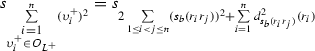
Now, we firstly determine the trace of the general product-connectivity matrices \(PC_{\alpha }({\mathcal {M}})\), \(PC_{\alpha }^{2}({\mathcal {M}})\), \(PC_{\alpha }^{3}({\mathcal {M}}),\) and \(PC_{\alpha }^{4}({\mathcal {M}})\) under Lq-ROF environment, i.e., \({s}_{tr(PC_{\alpha }({\mathcal {M}}))}\), \({s}_{tr(PC_{\alpha }^{2}({\mathcal {M}}))}\), \({s}_{tr(PC_{\alpha }^{3}({\mathcal {M}}))}\), and \({s}_{tr(PC_{\alpha }^{4}({\mathcal {M}}))}\). Moreover, using these equalities the upper and lower bounds for general product-connectivity energy are obtained.
Lemma 1
Let \({\mathcal {M}}=({\mathcal {L}},{\mathcal {E}})\) be a Lq-ROFG on n vertices and \(PC_{\alpha }({\mathcal {M}})=(PC_{\alpha }({{s}_{{a}_{{\mathcal {E}}}}} (r_{i}r_{j})),PC_{\alpha }({{s}_{{b}_{{\mathcal {E}}}}}(r_{i}r_{j})))\) be the general product-connectivity matrix of \({\mathcal {M}}\). Then,
-
1.
\({s}_{tr(PC_{\alpha }({\mathcal {M}}))}={s}_{0}\),
-
2.
\({s}_{tr(PC_{\alpha }^{2}({\mathcal {M}}))} = {s}_{2\sum \limits _{i\sim j}({d_{{\mathcal {M}}}(r_{i})d_{{\mathcal {M}}}(r_{j})})^{2\alpha }}\),
-
3.
\({s}_{tr(PC_{\alpha }^{3}({\mathcal {M}}))} = {s}_{2\sum \limits _{i\sim j}({d_{{\mathcal {M}}}(r_{i})d_{{\mathcal {M}}}(r_{j})})^{2\alpha }\left( \sum \limits _{\begin{array}{c} k\sim i\\ k\sim j \end{array}}{d^{2\alpha }_{{\mathcal {M}}}(r_{k})}\right) }\),
-
4.
\({s}_{tr(PC_{\alpha }^{4}({\mathcal {M}}))} = \quad {s}_{\sum \limits _{i=1}^{n} \left( \sum \limits _{i\sim j}({d_{{\mathcal {M}}}(r_{i})d_{{\mathcal {M}}}(r_{j})})^{2\alpha }\right) ^{2}}+{\sum \limits _{i\ne j}({d_{{\mathcal {M}}}(r_{i})d_{{\mathcal {M}}}(r_{j})})^{2\alpha }\left( \sum \limits _{\begin{array}{c} k\sim i\\ k\sim j \end{array}}{d^{2\alpha }_{{\mathcal {M}}}(r_{k})}\right) ^{2}}\).
Proof
1. Obvious.
2. For matrix \(PC_{\alpha }^{2}({\mathcal {M}})\). If \(i=j\)
whereas if \(i \ne j\)
Therefore, \({s}_{tr(PC^{2}_{\alpha }({{s}_{{a}_{{\mathcal {E}}}}}))}={s}_{\sum \limits _{i = 1}^{n}PC^{2}_{\alpha } ({{s}_{{a}_{{\mathcal {E}}}}}{(r_{i}r_{i})})}\)
\(={s}_{\sum \limits _{i = 1}^{n}\sum \limits _{i\sim j}({d_{{s}_{a}}(r_{i})d_{{s}_{a}}(r_{j})})^{2\alpha }} = {s}_{2 \sum \limits _{i\sim j}({d_{{s}_{a}}(r_{i})d_{{s}_{a}}(r_{j})})^{2\alpha }}\).
Similarly, we can show that
Hence, \({s}_{tr(PC^{2}_{\alpha }({\mathcal {M}}))} = {s}_{2\sum \limits _{i\sim j}({d_{{\mathcal {M}}}(r_{i})d_{{\mathcal {M}}}(r_{j})})^{2\alpha }}\).
3. The diagonal elements of \(PC^{3}_{\alpha }({\mathcal {M}})\) are
Therefore,
Similarly, we can show that
Hence, \({s}_{tr(PC^{3}({\mathcal {M}}))} = {s}_{2\sum \limits _{i\sim j}({d_{{\mathcal {M}}}(r_{i})d_{{\mathcal {M}}}(r_{j})})^{2\alpha }\left( \sum \limits _{\begin{array}{c} k\sim i\\ k\sim j \end{array}}{d^{2\alpha }_{{\mathcal {M}}}(r_{k})}\right) }.\)
We now calculate \({s}_{tr(PC^{4}_{\alpha })({{{s}_{{a}_{{\mathcal {E}}}}}}{(r_{i}r_{j})})}\). Because \(tr(PC^{4}_{\alpha })({{s}_{{a}_{{\mathcal {E}}}}}{(r_{i}r_{j})}) = \Vert (PC^{2}_{\alpha })({{s}_{{a}_{{\mathcal {E}}}}}{(r_{i}r_{j})})\Vert _{F}^{2}\), where \(\Vert (PC^{2}_{\alpha })({{s}_{{a}_{{\mathcal {E}}}}}{(r_{i}r_{j})})\Vert _{F}\) denotes the Frobenius norm of \((PC^{2}_{\alpha }({{s}_{{a}_{{\mathcal {E}}}}}{(r_{i}r_{i})}))\), we obtain
Similarly, we can show that
Hence, \({s}_{tr(PC^{4}_{\alpha }({\mathcal {M}}))} =\)
\({s}_{\sum \limits _{i=1}^{n} \left( \sum \limits _{i\sim j}({d_{{\mathcal {M}}}(r_{i})d_{{\mathcal {M}}}(r_{j})})^{2\alpha }\right) ^{2}+\sum \limits _{i\ne j}({d_{{\mathcal {M}}}(r_{i})d_{{\mathcal {M}}}(r_{j})})^{2\alpha }\left( \sum \limits _{\begin{array}{c} k\sim i\\ k\sim j \end{array}}{d^{2\alpha }_{{\mathcal {M}}}(r_{k})}\right) ^{2}}\). \(\square \)
Theorem 1
Let \({\mathcal {M}}=({\mathcal {L}},{\mathcal {E}})\) be a Lq-ROFG on n vertices. Then,
Furthermore, \({s}_{PCE_{\alpha }({\mathcal {M}})} ={s}_{\sqrt{2n\sum \limits _{i\sim j}({d_{{\mathcal {M}}}(r_{i})d_{{\mathcal {M}}}(r_{j})}})^{\alpha }}\) if and only if \({\mathcal {M}}\) is a graph with only isolated vertices, or end vertices.
Proof
The variance of the numbers \(~|\kappa ^{(\alpha )}_{i}|=\frac{{1}}{n}\sum \limits _{i = 1}^{n}|\kappa ^{(\alpha )}_{i}|^{2}- \left( \frac{{1}}{n}\sum \limits _{i = 1}^{n}|\kappa ^{(\alpha )}_{i}|\right) ^{2}\ge 0,~ i = 1,2, \ldots , n,\) therefore
If \({\mathcal {M}}\) is a graph with only isolated vertices, i.e., without edges, then \(\kappa _{i}^{(\alpha )}= 0\) for all \(i = 1,2, \ldots , n\), and therefore \(PCE({{s}_{{a}_{{\mathcal {E}}}}}{(r_{i}r_{j})}) = 0\). Since no vertices are adjacent, \(\sum \limits _{i\sim j}({d_{{s}_{a}}(r_{i})d_{{s}_{a}}(r_{j})})^{\alpha }=0\). If \({\mathcal {M}}\) is a graph with only end vertices, i.e., having degree one, then \(\kappa _{i}^{(\alpha )}\) = \(\pm d^{\alpha }_{{s}_{a}}(r_{i})\), so the variance of \(|\kappa _{i}^{(\alpha )}|=0\), \(i = 1,2, \ldots , n\). Thus, \( {s}_{(PCE_\alpha )({{s}_{{a}_{{\mathcal {E}}}}}{(r_{i}r_{j})})}={s}_{\sqrt{2n\sum \limits _{i\sim j}({d_{{s}_{a}}(r_{i})d_{{s}_{a}}(r_{j})}})^{\alpha }}.\)
Analogously, we can show that \({s}_{PCE_{\alpha }({{s}_{{b}_{{\mathcal {E}}}}}{(r_{i}r_{j})})}\le \)
\({s}_{\sqrt{2n\sum \limits _{i\sim j}({d_{{s}_{b}}(r_{i})d_{{s}_{b}}(r_{j})})^{\alpha }}}.\)
Hence, \({s}_{PCE_{\alpha }({\mathcal {M}})}\le {s}_{\sqrt{2n\sum \limits _{i\sim j}({d_{{\mathcal {M}}}(r_{i})d_{{\mathcal {M}}}(r_{j})}})^{\alpha }}.\) \(\square \)
Theorem 2
Let \(\mathcal {{\mathcal {M}}}=({\mathcal {L}},{\mathcal {E}})\) be a Lq-ROFG on n vertices and at least one edge. Then,
Proof
According to the Hölder inequality
which holds for any real numbers \(l_{i}, m_{i}\ge 0\), \(i = 1,2, \ldots \), n. Setting \(l_{i}=|\kappa _{i}^{(\alpha )}|^{\frac{2}{3}}\) , \(m_{i} =|\kappa _{i}^{(\alpha )}|^{\frac{4}{3}}\), p = \(\frac{3}{2}\), and \(q = 3\), we obtain
If the Lq-ROFG \({\mathcal {M}}\) has at least one edge, then all \(\kappa _{i}^{(\alpha )}\)’s are not equal to zero. Then, \(\sum \limits _{i = 1}^{n}|\kappa _{i}^{(\alpha )}|^{4} \ne 0\) and
By using Lemma 1, we get
\(\square \)
Theorem 3
Let \(\mathcal {{\mathcal {M}}}=({\mathcal {L}},{\mathcal {E}})\) be a Lq-ROFG on n vertices. If \({\mathcal {M}}\) is regular of degree \((p,q), p,q>0\), then
Proof
Suppose that \({\mathcal {M}}\) is a regular Lq-ROFG of degree \((p^{(2\alpha )},q^{(2\alpha )}) (p,q>0)\), i.e., \(d_{{s}_{a}}(r_{1}) =d_{{s}_{a}}(r_{2})=\ldots =d_{{s}_{a}}(r_{n}) = p^{2\alpha }\). Then, all nonzero entries of \((PC_{\alpha })({{s}_{{a}_{{\mathcal {E}}}}}{(r_{i}r_{i})})\) are equal to \({p^{(2\alpha )}}\), implying that \((PC_{\alpha })({{s}_{{a}_{{\mathcal {E}}}}}{(r_{i}r_{i})})={p^{(2\alpha )}}A({{s}_{{a}_{{\mathcal {E}}}}}{(r_{i}r_{i})})\). Therefore, for all \(i = 1,2, \ldots , n\)
Similarly, we can show that \({s}_{PCE_\alpha ({{s}_{{b}_{{\mathcal {E}}}}}{(r_{i}r_{j})})} = {s}_{{q^{(2\alpha )}}E({{s}_{{b}_{{\mathcal {E}}}}}{(r_{i}r_{j})})}.\)
Hence
\(\square \)
3.2 Laplacian energy of Lq-ROFGs
This subsection describes and determines Laplacian energy of Lq-ROFGs and provides descriptions of its properties.
Definition 11
The degree matrix, \(D({\mathcal {M}})=(D({s}_{{a}_{{\mathcal {E}}}}(r_{i}r_{j})),D({s}_{{b}_{{\mathcal {E}}}}(r_{i}r_{j})))=[d_{ij}],\) of a Lq-ROFG \({\mathcal {M}}=({\mathcal {L}},{\mathcal {E}})\) on n vertices, is a \(n\times n\) diagonal matrix defined as:
Definition 12
The Laplacian matrix (LM) of a Lq-ROFG \({\mathcal {M}}=({\mathcal {L}},{\mathcal {E}})\) is defined as:
where \(A({\mathcal {M}})\) and \(D({\mathcal {M}})\) are the adjacency matrix and the degree matrix of a Lq-ROFG \({\mathcal {M}}\), respectively.
Definition 13
The Laplacian energy of a Lq-ROFG \({\mathcal {M}}=({\mathcal {L}},{\mathcal {E}})\) is defined as:
where \(N_{L}\) and \(O_{L}\) are the sets of Laplacian eigenvalues of \(L({s}_{{a}_{{\mathcal {E}}}}(r_{i}r_{j}))\) and \(L({s}_{{b}_{{\mathcal {E}}}}(r_{i}r_{j}))\), respectively, and
where \(\varsigma _{i}\) and \(\upsilon _{i}\) represent eigenvalues of LM.
Theorem 4
Let \({\mathcal {M}}=({\mathcal {L}},{\mathcal {E}})\) be a Lq-ROFG with CLTS \(S=\{{s}_{\gamma }|\gamma =0, 1,\ldots , \tau \}\), and let \(L({\mathcal {M}})\) be the LM of \({\mathcal {M}}\). If \(\varsigma _{1}\ge \varsigma _{2}\ge \ldots \ge \varsigma _{n}\) and \(\upsilon _{1}\ge \upsilon _{2}\ge \ldots \ge \upsilon _{n}\) are the eigenvalues of \(L({s}_{{a}_{{\mathcal {E}}}}(r_{i}r_{j}))\) and \(L({s}_{{b}_{{\mathcal {E}}}}(r_{i}r_{j}))\), respectively, and \(\varpi _{i}=\varsigma _{i}-\frac{2\sum \limits _{1\le i<j\le n}{s}_{{a}_{{\mathcal {E}}}}(r_{i}r_{j})}{n},~~ \eta _{i}=\upsilon _{i}-\frac{2\sum \limits _{1\le i<j\le n}{s}_{{b}_{{\mathcal {E}}}}(r_{i}r_{j})}{n},\) then
where
Example 3
Let \({\mathcal {M}}=({\mathcal {L}},{\mathcal {E}})\) be a L6-ROFG on \(V=\{f_{1}, f_{2}, f_{3},f_{4},f_{5},f_{6},f_{7},f_{8},f_{9},f_{10}\}\) and \(E=\{f_{1}f_{2},f_{1}f_{6},f_{1}f_{7},f_{2}f_{3}, f_{2}f_{8},\) \(f_{3}f_{4},f_{3}f_{10},f_{4}f_{5},f_{4}f_{10}, f_{5}f_{6},f_{5}f_{9},f_{6}f_{7},\) \(f_{7}f_{8},f_{8}f_{9},f_{9}f_{10}\}\) with CLTS as \(S=\{{s}_{0}= \hbox {worst}\), \({s}_{1} = \hbox {very bad}\), \({s}_{2} = \hbox {bad}\), \({s}_{3} = \hbox {below average}\), \({s}_{4} = \hbox {average}\), \({s}_{5} =\hbox {above average}\), \({s}_{6} =\hbox {good}\), \({s}_{7}=\hbox {very good}\), \({s}_{8}=\hbox {exceptional}\}\), as shown in Fig. 6.

Linguistic 6-rung orthopair fuzzy graph with CLTS \(S=\{{s}_{\gamma }|\gamma \in [0, 8]\}\)
The adjacency matrix, degree matrix and LM of the L6-ROFG given in Fig. 6 are as follows:
The Laplacian spectrum and the Laplacian energy of a L6-ROFG \({\mathcal {M}}\), given in Fig. 6, are as follows:
and \(LE({\mathcal {M}}) = ({s}_{68.3128},{s}_{91.7360})\).
Furthermore, we have
Theorem 5
Let \({\mathcal {M}}=({\mathcal {L}},{\mathcal {E}})\) be a Lq-ROFG, and let \(L({\mathcal {M}})\) be the LM of \({\mathcal {M}}\) with CLTS \(S=\{{s}_{\gamma }|\gamma =0, 1,\ldots , \tau \}\). If \(\varsigma _{1}\ge \varsigma _{2}\ge \ldots \ge \varsigma _{n}\) and \(\upsilon _{1}\ge \upsilon _{2}\ge \ldots \ge \upsilon _{n}\) are the eigenvalues of \(L({s}_{{a}_{{\mathcal {E}}}}(r_{i}r_{j}))\) and \(L({s}_{{b}_{{\mathcal {E}}}}(r_{i}r_{j}))\), respectively, then
-
(i)
\({s}_{\sum \limits _{\begin{array}{c} i{=}1\\ \varsigma _{i}\in N_{L} \end{array}}^{n}\varsigma _{i}}\!\! ={s}_{2\sum \limits _{1\le i{<}j\le n}{s}_{{a}_{{\mathcal {E}}}}(r_{i}r_{j})},{s}_{\sum \limits _{\begin{array}{c} i{=}1\\ \upsilon _{i}\in O_{L} \end{array}}^{n}\upsilon _{i}}={s}_{2\sum \limits _{1\le i<j\le n}{s}_{{b}_{{\mathcal {E}}}}(r_{i}r_{j})}.\)
-
(ii)
\({s}_{\sum \limits _{\begin{array}{c} i=1\\ \varsigma _{i}\in N_{L} \end{array}}^{n}\varsigma _{i}^{2}}={s}_{2\sum \limits _{1\le i<j\le n}({s}_{{a}_{{\mathcal {E}}}}(r_{i}r_{j}))^{2}+\sum \limits _{i=1}^{n}d^{2}_{{s}_{{a}_{{\mathcal {E}}}}(r_{i}r_{j})}(r_{i})}\), \({s}_{\sum \limits _{\begin{array}{c} i{=}1\\ \upsilon _{i}\in O_{L} \end{array}}^{n}\upsilon _{i}^{2}} ={s}_{2\sum \limits _{1\le i<j\le n}({s}_{{b}_{{\mathcal {E}}}}(r_{i}r_{j}))^{2}+\sum \limits _{i=1}^{n}d^{2}_{{s}_{{b}_{{\mathcal {E}}}}(r_{i}r_{j})}(r_{i})}\).
Proof
-
(i)
Since LM of Lq-ROFG \(L({\mathcal {M}})\) is symmetric and its eigenvalues are nonnegative, we have
$$\begin{aligned} {s}_{\sum \limits _{\begin{array}{c} i=1\\ \varsigma _{i}\in N_{L} \end{array}}^{n}\varsigma _{i}}= & {} {s}_{tr(L({\mathcal {M}}))}\\= & {} {s}_{\sum \limits _{i=1}^{n}d_{{s}_{{a}_{{\mathcal {E}}}}(r_{i}r_{j})}(r_{i})}={s}_{2\sum \limits _{1\le i<j\le n}{s}_{{a}_{{\mathcal {E}}}}(r_{i}r_{j})}. \end{aligned}$$Therefore, \({s}_{\sum \limits _{\begin{array}{c} i=1\\ \varsigma _{i}\in N_{L} \end{array}}^{n}\varsigma _{i}}={s}_{2\sum \limits _{1\le i<j\le n}{s}_{{a}_{{\mathcal {E}}}}(r_{i}r_{j})}\).
Analogously, \({s}_{\sum \limits _{\begin{array}{c} i=1\\ \upsilon _{i}\in O_{L} \end{array}}^{n}\upsilon _{i}}={s}_{2\sum \limits _{1\le i<j\le n}{s}_{{b}_{{\mathcal {E}}}}(r_{i}r_{j})}\).
-
(ii)
Utilizing Definition 12, we get:
$$\begin{aligned}&L({s}_{{a}_{{\mathcal {E}}}}(r_{i}r_{j}))\\&\quad =\left[ \begin{array}{llll} d_{{s}_{{a}_{{\mathcal {E}}}}(r_{i}r_{j})}(r_{1}) &{} -{s}_{{a}_{{\mathcal {E}}}}(r_{1}r_{2}) &{} \ldots &{} -{s}_{{a}_{{\mathcal {E}}}}(r_{1}r_{n}) \\ -{s}_{{a}_{{\mathcal {E}}}}(r_{2}r_{1}) &{} d_{{s}_{{a}_{{\mathcal {E}}}}(r_{i}r_{j})}(r_{2}) &{} \ldots &{} -{s}_{{a}_{{\mathcal {E}}}}(r_{2}r_{n}) \\ \vdots &{} \vdots &{} \ddots &{} \vdots \\ -{s}_{{a}_{{\mathcal {E}}}}(r_{n}r_{1}) &{} -{s}_{{a}_{{\mathcal {E}}}}(r_{n}r_{2}) &{} \ldots &{} d_{{s}_{{a}_{{\mathcal {E}}}}(r_{i}r_{j})}(r_{n}) \end{array} \right] . \end{aligned}$$
Based on matrix trace properties, we have
where
So,
Similarly, we can easily show that
\(\square \)
Theorem 6
If the Lq-ROFG \({\mathcal {M}}=({\mathcal {L}},{\mathcal {E}})\) with CLTS \(S=\{{s}_{\gamma }|\gamma =0, 1,\ldots , \tau \}\) is regular, then
-
(i)
\({s}_{LE({s}_{{a}_{{\mathcal {E}}}}(r_{i}r_{j}))}\le {s}_{|\varpi _{1}|+\sqrt{(n-1)\left( 2\sum \limits _{1\le i<j\le n}({s}_{{a}_{{\mathcal {E}}}}(r_{i}r_{j}))^{2}-\varpi _{1}^{2}\right) }};\)
-
(ii)
\({s}_{LE({s}_{{b}_{{\mathcal {E}}}}(r_{i}r_{j}))}\le {s}_{|\eta _{1}|+\sqrt{(n-1)\left( 2\sum \limits _{1\le i<j\le n}({s}_{{b}_{{\mathcal {E}}}}(r_{i}r_{j}))^{2}-\eta _{1}^{2}\right) }}.\)
3.3 Signless Laplacian energy of Lq-ROFGs
In this subsection, we introduce a novel concept of signless Laplacian energy of Lq-ROFGs and provide descriptions of its properties.
Definition 14
The signless Laplacian matrix (SLM) of a Lq-ROFG \({\mathcal {M}}=({\mathcal {L}},{\mathcal {E}})\) is defined as \(L^{+}({\mathcal {M}})= \langle L^{+}({s}_{a})(r_{i}r_{j})), L^{+}({s}_{b}(r_{i}r_{j}))\rangle =D({\mathcal {M}})+A({\mathcal {M}})\), where \(D({\mathcal {M}})\) is the degree matrix and \(A({\mathcal {M}})\) is the adjacency matrix of \({\mathcal {M}}\).
Definition 15
The signless Laplacian energy of Lq-ROFG \({\mathcal {M}}=({\mathcal {L}},{\mathcal {E}})\) is defined as
where \(N_{L^{+}}\) and \(O_{L^{+}}\) are the sets of signless Laplacian eigenvalues of \(L^{+}({s}_{a}(r_{i}r_{j}))\), \(L^{+}({s}_{b}(r_{i}r_{j}))\), respectively, and
where \(\varsigma ^{+}_{i}\) and \(\upsilon ^{+}_{i}\) are the eigenvalues of SLM.
Theorem 7
Let \({\mathcal {M}}=({\mathcal {L}},{\mathcal {E}})\) be a Lq-ROFG with CLTS \(S=\{{s}_{\gamma }|\gamma =0, 1,\ldots , \tau \}\) and let \(L^{+}({\mathcal {M}})\) be the SLM of \({\mathcal {M}}\). If \(\varsigma ^{+}_{1}\ge \varsigma ^{+}_{2}\ge \ldots \ge \varsigma ^{+}_{n}\) and \(\upsilon ^{+}_{1}\ge \upsilon ^{+}_{2}\ge \ldots \ge \upsilon ^{+}_{n}\) are the eigenvalues of \(L^{+}({s}_{a}(r_{i}r_{j}))\) and \(L^{+}({s}_{b}(r_{i}r_{j}))\), respectively, and \(\varpi ^{+}_{i}=\varsigma ^{+}_{i}-\frac{2\sum \limits _{1\le i<j\le n}{s}_{a}(r_{i}r_{j})}{n},~~ \eta ^{+}_{i}=\upsilon ^{+}_{i}-\frac{2\sum \limits _{1\le i<j\le n}{s}_{b}(r_{i}r_{j})}{n}.\) Then
where
Example 4
Let \({\mathcal {M}}=({\mathcal {L}},{\mathcal {E}})\) be a L6-ROFG on \(V=\{f_{1}, f_{2}, f_{3},f_{4},f_{5},f_{6},f_{7},f_{8}\}\) and \(E=\{f_{1}f_{2},f_{1}f_{6},f_{1}f_{7},\) \(f_{2}f_{3},f_{2}f_{8},f_{3}f_{4}, f_{3}f_{8},\) \(f_{4}f_{5},f_{4}f_{8},f_{5}f_{6}, f_{5}f_{7},f_{6}f_{7}\}\) with CLTS as \(S=\{{s}_{0}= \hbox {worst}\), \({s}_{1} = \hbox {very bad}\), \({s}_{2} = \hbox {bad}\), \({s}_{3} = \hbox {below average}\), \({s}_{4} = \hbox {average}\), \({s}_{5} =\hbox {above average}\), \({s}_{6} =\hbox {good}\), \({s}_{7}=\hbox {very good}\), \({s}_{8}=\hbox {exceptional}\}\), as shown in Fig. 7.
The adjacency matrix, degree matrix and SLM of the L6-ROFG given in Fig. 7 are as follows:
The signless Laplacian spectrum and the signless Laplacian energy of a L6-ROFG \({\mathcal {M}}\), shown in Fig. 7, are as follows:

Linguistic 6-rung orthopair fuzzy graph with CLTS \(S=\{{s}_{\gamma }|\gamma \in [0, 8]\}\)
and \(LE^{+}({\mathcal {M}})=({s}_{45.0446},{s}_{71.8214})\).
Furthermore,
Theorem 8
Let \({\mathcal {M}}=({\mathcal {L}},{\mathcal {E}})\) be a graph with CLTS \(S=\{{s}_{\gamma }|\gamma =0, 1,\ldots , \tau \}\) and let \(L^{+}({\mathcal {M}})\) be the SLM of \({\mathcal {M}}\). If \(\varsigma ^{+}_{1}\ge \varsigma ^{+}_{2}\ge \ldots \ge \varsigma ^{+}_{n}\) and \(\upsilon ^{+}_{1}\ge \upsilon ^{+}_{2}\ge \ldots \ge \upsilon ^{+}_{n}\) are the eigenvalues of \(L^{+}({s}_{a}(r_{i}r_{j}))\) and \(L^{+}({s}_{b}(r_{i}r_{j}))\), respectively. Then
- (i):
-

- (ii):
-
 ,
,  .
.

 ,
,  .
.Proof
Proof of this theorem follows Theorem 5. \(\square \)
4 Spectra of Lq-ROFDGs
Concepts of product-connectivity energy, generalized product-connectivity energy, Laplacian energy and signless Laplacian energy of Lq-ROFGs to Lq-ROFDGs are generalized in this section. As adjacency matrix of Lq-ROFDG is not necessarily symmetric, its eigenvalues might be complex numbers.
4.1 Generalized product-connectivity energy of Lq-ROFDGs
Definition 16
Let \({\mathcal {D}}=({\mathcal {L}},\overrightarrow{{\mathcal {E}}})\) be a Lq-ROFDG on n vertices. The general product-connectivity matrix, \(PC_{\alpha }({\mathcal {D}})=(PC_{\alpha }({s}_{{a}_{\overrightarrow{{\mathcal {E}}}}}(r_{i}r_{j})), PC_{\alpha }({s}_{{b}_{\overrightarrow{{\mathcal {E}}}}}(r_{i}r_{j})))=[d_{ij}],\) of \({\mathcal {D}}\) is a \(n\times n\) matrix defined as:
Definition 17
Let \({\mathcal {D}}=({\mathcal {L}},\overrightarrow{{\mathcal {E}}})\) be a Lq-ROFDG on n vertices. The general product-connectivity energy of \({\mathcal {D}}\) is defined as:
where \({\mathcal {N}}\) and \({\mathcal {O}}\) are the sets of eigenvalues of \(PC_{\alpha }({s}_{{a}_{\overrightarrow{{\mathcal {E}}}}}(r_{i}r_{j}))\) and \(PC_{\alpha }({s}_{{b}_{\overrightarrow{{\mathcal {E}}}}}(r_{i}r_{j}))\), respectively, and \(\text {Re}({\tilde{t}}_{i})\) and \(\text {Re}({\tilde{w}}_{i})\) represent the real part of eigenvalues \({\tilde{t}}_{i}\) and \({\tilde{w}}_{i}\), respectively.

L5-ROFDG with CLTS \(S=\{{s}_{\gamma }|\gamma \in [0, 8]\}\)
Theorem 9
Let \({\mathcal {D}}=({\mathcal {L}},\overrightarrow{{\mathcal {E}}})\) be a Lq-ROFDG with CLTS \(S=\{{s}_{\gamma }|\gamma =0, 1,\ldots , \tau \}\) and \(PC_{\alpha }({\mathcal {D}})\) be its adjacency matrix. If \({\tilde{t}}_{1}\ge {\tilde{t}}_{2}\ge \ldots \ge {\tilde{t}}_{n}\) and \({\tilde{w}}_{1}\ge {\tilde{w}}_{2}\ge \ldots \ge {\tilde{w}}_{n}\) are the eigenvalues of \(PC_{\alpha }({s}_{{a}_{\overrightarrow{{\mathcal {E}}}}}(r_{i}r_{j}))\) and \(PC_{\alpha }({s}_{{b}_{\overrightarrow{{\mathcal {E}}}}}(r_{i}r_{j}))\), respectively, then
Example 5
Consider a digraph \(D=(V, \overrightarrow{E}),\) where \(V=\{f_{1},f_{2},f_{3},f_{4},f_{5}\), \(f_{6},f_{7},f_{8},f_{9}\}\) and \(\overrightarrow{E}=\{f_{1}f_{2},f_{1}f_{6}\), \(f_{1}f_{7},f_{2}f_{3}\), \(f_{3}f_{8},f_{3}f_{9}\), \(f_{4}f_{3},f_{5}f_{4}\), \(f_{5}f_{7},f_{6}f_{5}\), \(f_{6}f_{8},f_{7}f_{9}\), \(f_{8}f_{1},f_{8}f_{2},f_{8}f_{9}\), \(f_{9}f_{4},f_{9}f_{5}\}\) with CLTS as \(S=\{{s}_{0}= \hbox {worst}\), \({s}_{1} = \hbox {very bad}\), \({s}_{2} = \hbox {bad}\), \({s}_{3} = \hbox {below average}\), \({s}_{4} = \hbox {average}\), \({s}_{5} =\hbox {above average}\), \({s}_{6} =\hbox {good}\), \({s}_{7}=\hbox {very good}\), \({s}_{8}=\hbox {exceptional}\}\). Let \({\mathcal {D}}=({\mathcal {L}},\overrightarrow{{\mathcal {E}}})\) be a L5-ROFDG on V, as shown in Fig. 8.
The adjacency matrix of a L5-ROFDG given in Fig. 8 is:
The generalized product-connectivity matrix with \(\alpha =-1/2\) of a L5-ROFDG \(PC({\mathcal {D}})\), shown in Fig. 8, is:
The spectrum and the energy values of a Lq-ROFDG \({\mathcal {D}}\), given in Fig. 8, are as follows:
Therefore,
Now, \(PCE_{-1/2}({s}_{{a}_{{\mathcal {E}}}}(r_{i}r_{j}))= {s}_{1.1481}\) and \(PCE_{-1/2}({s}_{{b}_{{\mathcal {E}}}}(r_{i}r_{j}))= {s}_{0.5209}\).
Therefore, \(PCE_{-1/2}({\mathcal {D}})=({s}_{1.1481},{s}_{0.5209})\).
Furthermore,
4.2 Laplacian energy of Lq-ROFDGs
This subsection discusses the Laplacian energy of Lq-ROFDGs.
Definition 18
Let \({\mathcal {D}}=({\mathcal {L}},\overrightarrow{{\mathcal {E}}})\) be a Lq-ROFDG on n vertices. The degree matrix, \(D({\mathcal {D}})=(D({s}_{{a}_{\overrightarrow{{\mathcal {E}}}}}(r_{i}r_{j})), D({s}_{{b}_{\overrightarrow{{\mathcal {E}}}}}(r_{i}r_{j})))=[\text {d}_{ij}],\) of \({\mathcal {D}}\) is a \(n\times n\) diagonal matrix defined as:
Definition 19
The Laplacian matrix (LM) of a Lq-ROFDG \({\mathcal {D}}=({\mathcal {L}},\overrightarrow{{\mathcal {E}}})\) is defined as \(L({\mathcal {D}})=(L({s}_{{a}_{\overrightarrow{{\mathcal {E}}}}}(r_{i}r_{j})), L({s}_{{b}_{\overrightarrow{{\mathcal {E}}}}}(r_{i}r_{j}))) = D^{\text {out}}({\mathcal {D}})-A({\mathcal {D}})\), where \(A({\mathcal {D}})\) is an adjacency matrix and \(D^{\text {out}}({\mathcal {D}})\) is an out-degree matrix of \({\mathcal {D}}\).
Definition 20
The Laplacian energy of a Lq-ROFDG \({\mathcal {D}}=({\mathcal {L}},\overrightarrow{{\mathcal {E}}})\) is defined as:
where \({\mathcal {N}}_{L}\) and \({\mathcal {O}}_{L}\) are the sets of Laplacian eigenvalues of \(L({s}_{{a}_{\overrightarrow{{\mathcal {E}}}}}(r_{i}r_{j}))\) and \(L({s}_{{b}_{\overrightarrow{{\mathcal {E}}}}}(r_{i}r_{j}))\), respectively, and
where \(\text {Re}(\mathfrak {R}_{i})\) and \(\text {Re}(\hbar _{i})\) are the real parts of the eigenvalues of LM.
Theorem 10
Let \({\mathcal {D}}=({\mathcal {L}},\overrightarrow{{\mathcal {E}}})\) be a Lq-ROFDG with CLTS \(S=\{{s}_{\gamma }|\gamma =0, 1,\ldots , \tau \}\), and let \(L({\mathcal {D}})\) be the LM of \({\mathcal {D}}\). If \(\mathfrak {R}_{1}\ge \mathfrak {R}_{2}\ge \ldots \ge \mathfrak {R}_{n}\) and \( \hbar _{1}\ge \hbar _{2}\ge \ldots \ge \hbar _{n}\) are the eigenvalues of \(L({s}_{{a}_{\overrightarrow{{\mathcal {E}}}}}(r_{i}r_{j}))\) and \(L({s}_{{b}_{\overrightarrow{{\mathcal {E}}}}}(r_{i}r_{j}))\), respectively, then
Theorem 11
Let \({\mathcal {D}}=({\mathcal {L}},\overrightarrow{{\mathcal {E}}})\) be a Lq-ROFDG with CLTS \(S=\{{s}_{\gamma }|\gamma =0, 1,\ldots , \tau \}\), and let \(L({\mathcal {D}})\) be the LM of \({\mathcal {D}}\). If \(\mathfrak {R}_{1}\ge \mathfrak {R}_{2}\ge \ldots \ge \mathfrak {R}_{n}\) and \( \hbar _{1}\ge \hbar _{2}\ge \ldots \ge \hbar _{n}\) are the eigenvalues of \(L({s}_{{a}_{\overrightarrow{{\mathcal {E}}}}}(r_{i}r_{j}))\) and \(L({s}_{{b}_{\overrightarrow{{\mathcal {E}}}}}(r_{i}r_{j}))\), respectively, and \( \wp _{i}=\text {Re}(\mathfrak {R}_{i})-\frac{\sum \limits _{1\le i<j\le n}{s}_{{a}_{\overrightarrow{{\mathcal {E}}}}}(r_{i}r_{j})}{n},~~ {\mathfrak {s}}_{i}= {\text {Re}}(\hbar _{i})-\frac{\sum \limits _{1\le i<j\le n}{s}_{{b}_{\overrightarrow{{\mathcal {E}}}}}(r_{i}r_{j})}{n},\) then \({s}_{\sum \limits _{i=1}^{n} \wp _{i}}={s}_{0},~~~{s}_{\sum \limits _{i=1}^{n} {\mathfrak {s}}_{i}}={s}_{0}\).
Example 6
The adjacency matrix is given in Example 5, but out-degree matrix and LM of the Lq-ROFDG shown in Fig. 8 are as follows:
The Laplacian spectrum and the Laplacian energy of a Lq-ROFDG \({\mathcal {D}}\), given in Fig. 8, are as follows:
and \(LE({\mathcal {D}})=({s}_{31.0714},{s}_{50.0349})\).
Furthermore, we have
4.3 Signless Laplacian energy of Lq-ROFDGs
We now discuss the signless Laplacian energy of Lq-ROFDGs and its properties.
Definition 21
The SLM of a Lq-ROFDG \({\mathcal {D}}=({\mathcal {L}},\overrightarrow{{\mathcal {E}}})\) is defined as \(L^{+}({\mathcal {D}})=(L^{+}({s}_{{a}_{\overrightarrow{{\mathcal {E}}}}}(r_{i}r_{j})), L^{+}({s}_{{b}_{\overrightarrow{{\mathcal {E}}}}}(r_{i}r_{j}))) =D^{\text {out}}({\mathcal {D}})+A({\mathcal {D}})\), where \(A({\mathcal {D}})\) and \(D^{\text {out}}({\mathcal {D}})\) are the adjacency matrix and out-degree matrix of \({\mathcal {D}}\), respectively.
Definition 22
The spectrum of the SLM of a Lq-ROFDG \(L^{+}({\mathcal {D}})\) is defined as \(({\mathcal {N}}_{L^{+}},{\mathcal {O}}_{L^{+}})\), where \({\mathcal {N}}_{L^{+}}\) and \({\mathcal {O}}_{L^{+}}\) are the sets of signless Laplacian eigenvalues of \(L^{+}({s}_{{a}_{\overrightarrow{{\mathcal {E}}}}}(r_{i}r_{j}))\) and \(L^{+}({s}_{{b}_{\overrightarrow{{\mathcal {E}}}}}(r_{i}r_{j}))\), respectively.
Definition 23
The energy of signless Laplacian of a Lq-ROFDG \({\mathcal {D}}=(\mathcal {L^{+}},\overrightarrow{{\mathcal {E}}})\) is defined as:
where \({\mathcal {N}}_{L^{+}}\) and \({\mathcal {O}}_{L^{+}}\) are the sets of signless Laplacian eigenvalues of \(L^{+}({s}_{{a}_{\overrightarrow{{\mathcal {E}}}}}(r_{i}r_{j}))\) and \(L^{+}({s}_{{b}_{\overrightarrow{{\mathcal {E}}}}}(r_{i}r_{j}))\), respectively, and
where \(\text {Re}(\mathfrak {R}_{i}^{+})\) and \(\text {Re}(\hbar _{i}^{+})\) are the real parts of eigenvalues of SLM.
Theorem 12
Let \({\mathcal {D}}=({\mathcal {L}},\overrightarrow{{\mathcal {E}}})\) be a Lq-ROFDG with CLTS \(S=\{{s}_{\gamma }|\gamma =0, 1,\ldots , \tau \}\), and let \(L^{+}({\mathcal {D}})\) be the SLM of \({\mathcal {D}}\). If \(\mathfrak {R}_{1}^{+}\ge \mathfrak {R}_{2}^{+}\ge \ldots \ge \mathfrak {R}_{n}^{+}\) and \( \hbar _{1}^{+}\ge \hbar _{2}^{+}\ge \ldots \ge \hbar _{n}^{+}\) are the eigenvalues of \(L^{+}({s}_{{a}_{\overrightarrow{{\mathcal {E}}}}}(r_{i}r_{j}))\) and \(L^{+}({s}_{{b}_{\overrightarrow{{\mathcal {E}}}}}(r_{i}r_{j}))\), respectively, then
Theorem 13
Let \({\mathcal {D}}=({\mathcal {L}},\overrightarrow{{\mathcal {E}}})\) be a Lq-ROFDG with CLTS \(S=\{{s}_{\gamma }|\gamma =0, 1,\ldots , \tau \}\), and let \(L^{+}({\mathcal {D}})\) be the SLM of \({\mathcal {D}}\). If \(\mathfrak {R}_{1}^{+}\ge \mathfrak {R}_{2}^{+}\ge \ldots \ge \mathfrak {R}_{n}^{+}\) and \( \hbar _{1}^{+}\ge \hbar _{2}^{+}\ge \ldots \ge \hbar _{n}^{+}\) are the eigenvalues of \(L^{+}({s}_{{a}_{\overrightarrow{{\mathcal {E}}}}}(r_{i}^{+}r_{j}))\) and \(L^{+}({s}_{{b}_{\overrightarrow{{\mathcal {E}}}}}(r_{i}^{+}r_{j}))\), respectively, and \( \wp _{i}^{+}=\text {Re}(\mathfrak {R}_{i}^{+})-\frac{\sum \limits _{1\le i<j\le n}{s}_{{a}_{\overrightarrow{{\mathcal {E}}}}}(r_{i}^{+}r_{j})}{n}, {\mathfrak {s}}_{i}^{+}=Re(\hbar _{i}^{+})-\frac{\sum \limits _{1\le i<j\le n}{s}_{{b}_{\overrightarrow{{\mathcal {E}}}}}(r_{i}^{+}r_{j})}{n},\) then \({s}_{\sum \limits _{i=1}^{n}\wp _{i}^{+}}={s}_{0},~~{s}_{\sum \limits _{i=1}^{n} {\mathfrak {s}}_{i}^{+}}={s}_{0}\).
Example 7
The adjacency matrix and out-degree matrix are shown in Examples 5 and 6, respectively, but SLM of the Lq-ROFDG shown in Fig. 8 is as follows:
The signless Laplacian spectrum and the signless Laplacian energy of a Lq-ROFDG \({\mathcal {D}}\), given in Fig. 8, are as follows:
and \(LE^{+}({\mathcal {D}})=({s}_{28.6778},{s}_{43.1785})\).
Furthermore, we have
5 A graph-based MAGDM approach with linguistic q-rung orthopair fuzzy information
In this section, the Lq-ROF Einstein averaging (Lq-ROFEA) operator is utilized to develop a novel graph-based MAGDM model.
In the MAGDM problems, let \(\ell =\{\ell _{1},\ell _{2},\ldots ,\ell _{n}\}\) be a discrete set of alternatives, \(e=\{e_{1},e_{2},\ldots ,e_{m}\}\) be the set of organization composed of many experts, and \(\omega =(\omega _{1}, \omega _{2}, \ldots , \omega _{m})^{T}\) be the weight vector satisfying \(\sum \limits _{k=1}^{m}\omega _{k}=1\) and \(\omega _{k}\ge 0, k=1,2, \ldots , m.\) Each expert in an organization provides preference relation for each pair of alternatives, so for each organization its linguistic q-rung orthopair fuzzy preference relation (Lq-ROFPR) is constructed with \(H^{(k)}=(p_{ij}^{(k)})_{n\times n}=({s}_{{a}_{ij}}^{(k)},{s}_{{b}_{ij}}^{(k)})_{n\times n}\).
-
Step 1.
We utilize the Lq-ROFEA operator to aggregate all \(p^{(k)}_{ij} (j=1, 2, \ldots , n)\) that correspond to the alternative \(\ell _{i}\). We get the Lq-ROFN \({p^{(k)}_{i}}\) of the alternative \(\ell _{i}\) over all the other alternatives for the organization \(e_{k}\).
$$\begin{aligned} p^{(k)}_{i}= & {} \text {L}q\text {-ROFEA}(p^{(k)}_{i1},p^{(k)}_{i2},\ldots ,p^{(k)}_{in})\\= & {} \left( {s}_{\tau \left( \frac{\prod _{i=1}^{n}\left( 1+\left( \frac{a_{i}}{\tau }\right) ^{q}\right) ^{\omega _{i}}- \prod _{i=1}^{n}\left( 1-\left( \frac{a_{i}}{\tau }\right) ^{q}\right) ^{\omega _{i}}}{\prod _{i=1}^{n}\left( 1+\left( \frac{a_{i}}{\tau }\right) ^{q}\right) ^{\omega _{i}}+ \prod _{i=1}^{n}\left( 1-\left( \frac{a_{i}}{\tau }\right) ^{q}\right) ^{\omega _{i}}}\right) ^{1/q}},\right. \\&\left. {s}_{\tau \left( \frac{2^{1/q}\prod _{i=1}^{n}\left( \frac{b_{i}}{\tau }\right) ^{\omega _{i}}}{\left( \prod _{i=1}^{n}\left( 2-\left( \frac{b_{i}}{\tau }\right) ^{q}\right) ^{\omega _{i}}+ \prod _{i=1}^{n}\left( \frac{b_{i}}{\tau }\right) ^{q\omega _{i}}\right) ^{1/q}}\right) }\right) . \end{aligned}$$ -
Step 2.
If the weight vector \(\omega =(\omega _{1}, \omega _{2}, \ldots , \omega _{m})^{T}\) of all organizations is known, then go to Step 4;
otherwise, the weight of each organization needs to be accounted for. To calculate the weights of decision organization, it proceeds as follows:
-
(i)
We first use the linguistic q-rung orthopair fuzzy Hamming distance (Lq-ROFHD) between two Lq-ROFNs to find out the weights of the experts
$$\begin{aligned}&D(p_{1},p_{2})=\frac{\tau }{2}\left( \left| \left( \frac{a_{p_{1}}}{\tau }\right) ^{q} -\left( \frac{a_{p_{2}}}{\tau }\right) ^{q}\right| \right. \nonumber \\&\qquad \left. +\,\left| \left( \frac{b_{p_{1}}}{\tau }\right) ^{q}-\left( \frac{b_{p_{2}}}{\tau }\right) ^{q}\right| \right. \nonumber \\&\qquad \left. +\,\left| \left( \frac{{s}_{{\pi }_{p_{1}}}}{\tau }\right) ^{q}-\left( \frac{{s}_{{\pi }_{p_{2}}}}{\tau }\right) ^{q}\right| \right) \nonumber \\&\quad \text {where} {s}_{{\pi }_{p_{1}}}=\root q \of {\tau ^{q}-a_{p_{1}}^{q}-b_{p_{1}}^{q}},\nonumber \\&\qquad {s}_{{\pi }_{p_{2}}}=\root q \of {\tau ^{q}-a_{p_{2}}^{q}-b_{p_{2}}^{q}} \end{aligned}$$(3)to obtain the difference matrices,
$$\begin{aligned}&D_{lk}=(d_{ij}^{(lk)})_{n \times n}=d(p_{ij}^{(l)},p_{ij}^{(k)})_{n \times n},\\&\quad l,k=1,2,\ldots , m \end{aligned}$$where
-
(a)
\(d_{ij}^{(lk)}\ge 0\), especially, if \(l=k\), then \(d_{ij}^{(lk)}=0, ~i,j=1, 2, \ldots , n\);
-
(b)
\(d_{ij}^{(lk)}=0, i=j\);
-
(c)
\(d_{ij}^{(lk)}=d_{ji}^{(lk)}\).
\(D_{lk}\) is a symmetric matrix and the values of diagonal elements are zero.
-
(a)
-
(ii)
Determine the average value of the matrix \(D_{lk}\) from
$$\begin{aligned} {\bar{d}}_{lk}=\frac{1}{n^{2}}\sum \limits _{i=1}^{n}\sum \limits _{j=1}^{n}d_{ij}^{(lk)} \end{aligned}$$(4) -
(iii)
Afterward, let \({\bar{d}}=\sum \limits _{k=1,k\ne l}^{m} {\bar{d}}_{lk}\), then
$$\begin{aligned} {{\bar{d}}}_{l}=\frac{1}{n^{2}}\sum \limits _{k=1,k\ne l}^{m}\sum \limits _{i=1}^{n}\sum \limits _{j=1}^{n}d_{ij}^{(lk)}, \end{aligned}$$(5)which denotes the deviation of the organization \(e_{l}\) from the rest organizations.
-
(iv)
The weight vector \(\omega _{l}\) of the organizations \(e_{l}\) can be calculated as
$$\begin{aligned} \omega _{l}=\frac{({\bar{d}}_{l})^{-1}}{\sum \limits _{l=1}^{m}({\bar{d}}_{l})^{-1}}, \quad l=1,2,\ldots ,m \end{aligned}$$(6)
-
(i)
-
Step 3.
To aggregate all \({p^{(k)}_{i}}~(k=1, 2, \ldots , m)\) into a collective Lq-ROFN \({p^{(k)}_{i}}\) for the alternative \(\ell _{i}\), use Lq-ROF Einstein weighted averaging (Lq-ROFEWA) operator.
-
Step 4.
Compute the score functions of \({p_{i}}~(i=1, 2, \ldots , n)\) by Eq. (1) to rank all the alternatives \(\ell _{i}(i=1, 2, \ldots , n)\) according to \({\mathcal {S}}(\ell _{i})(i=1, 2, \ldots , n)\).
The specific steps of this proposed approach to MAGDM are depicted in Fig. 9.

The specific steps of the proposed approach to MAGDM
5.1 Illustrative example and comparative analysis
In the following, a numerical example related to “mobile payment platform selection” is given to describe the validity of our approach:
5.1.1 Mobile payment platform selection
The advancement of disruptive technologies has made mobile devices acquire new functionalities that support multiple mobile financial services including bill payments, account transfers, person-to-person proximity payments, exchanges, remote payments, and other forms of services such as mobile ticketing and discounts (Liana-Cabanillas et al. 2018). There is a development, called “mobile payment technology,” which is undergoing rapid growth among the different mobile applications offered today. Mobile payment can be seen as an application between mobile devices and a payment mechanism that helps the user to pay for transaction through mobile devices. In sub-Saharan Africa, the adoption of mobile payment technology has been impressive, with various operators offering diverse services. As the beneficial impact mobile payment has on organizations, numerous mobile payment platforms have proliferated around the world. Assessment and selection of numerous mobile payment platforms is often difficult, as they require detailed identification. Also, because of uncertainty and vagueness in real-life situations, decision makers can find it difficult to examine the mobile payment platforms accurately. However, this problem can be solved using Lq-ROF MAGDM. An example related to selected mobile payment platform is used to illustrate proposed decision-making approach. A group of five decision makers \(\{e_{1},e_{2},e_{3},e_{4},e_{5}\}\), are invited to evaluate six mobile payment platforms MTN Mobile Money (MTN MM), M-Pesa (MP), Tigo Pesa (TP), Vodafone Cash (VC), Orange Money (OM), and Airtel Money (AM), i.e., alternatives \(\ell _{i}(i = 1,2, \ldots , 6).\) Here, we suppose that the decision makers have equal weights. In order to completely communicate the experts’ appreciation, linguistic variables can be added within the predefined LTS \(S=\{{s}_{0}=\) extremely bad, \({s}_{1}=\) very bad, \({s}_{2}=\) bad, \({s}_{3}=\) relatively bad, \({s}_{4}=\) normal, \({s}_{5}=\) relatively good, \({s}_{6}=\) good, \({s}_{7}=\) very good, \({s}_{8}=\) extraordinary}. The five decision makers \(e_{k}(k=1,2, , , , \ldots , 5)\) presented their assessments in L4-ROFPRs as follows:
The L4-ROFDGs \({\mathcal {D}}_{i}\) corresponding to L4-ROFPRs \(R_{k}~(k=1, 2, \ldots , 5)\) given in Tables 3, 4, 5, 6 and 7 are shown in Fig. 10.
Compute the averaged Lq-ROFN \(p^{(k)}_{i}\) of an alternative \(\ell _{i}\) over all the other alternatives for the experts \(e_{k}(k= 1, 2, \ldots , 5)\) using Lq-ROFEA operator, as in Table 8.
We first utilize Eq. (3) between two Lq-ROFNs to find out the weights of the experts to compute \(d(p_{ij}^{(l)},p_{ij}^{(k)}), i,j=1,2,\ldots ,6; l,k=1, 2,\ldots , 5\) and obtained the difference matrices as follows:
Utilize Eq. (4) to determine the average values of the difference matrices, as in Table 9.
Use Eq. (5) to determine the deviation of the expert \(e_{1}\) from the remaining experts as follows:

L4-ROFDG with CLTS \(S=\{{s}_{\gamma }|\gamma \in [0, 8]\}\)
Utilizing Eq. (6), we determine the weights of the experts.
Compute a collective Lq-ROFN \(p_{i}~(i=1,2,\ldots ,6)\) of the alternative \(\ell _{i}\) over all the other alternatives using Lq-ROFEWA operator.
Compute the score function of Lq-ROFN by Eq. (1) of \(p_{i}(i=1, 2, \ldots , 6)\), and rank all the alternatives \(\ell _{i}(i= 1, 2, \ldots , 6)\) according to the values of \({\mathcal {S}}(p_{i})(i = 1, 2, \ldots , 6)\).
Then, \(\ell _{3}\succ \ell _{4}\succ \ell _{5}\succ \ell _{1}\succ \ell _{2}\succ \ell _{6}\). Thus, the optimal choice is \(\ell _{3}.\) The curiosity of this decision-making approach is that by comparing graphical structures with Lq-ROF data, we have built up a MAGDM model with the interrelated organizations and depicted various connections among the organizations.
5.2 Validity analysis of the developed approach
In this subsection, to show the effectiveness and superiority of our developed approach, we utilize other existing techniques to handle with this example and compare the results with the developed approach.
From this analysis, it is easy to see that our developed method based on graph theory and Lq-ROF Einstein weighted averaging operator is more versatile and reasonable to solve MAGDM problems.
Following are the figures which best describe the above evaluations.
5.2.1 Further discussion
It can be seen from the above analysis that the ranking results of the above methods are same and the best alternative is \(\ell _3\). This verifies that the developed approach is reasonable and useful for MAGDM problems with Lq-ROFNs. Lq-ROFS is more and more general and contains more information in the MAGDM process. Therefore, our developed method provides more general and powerful information in MAGDM.
-
1.
Comparing with the Lq-ROF weighted averaging (Lq-ROFWA) operator (i.e., taking algebraic t-norm and t-conorm) proposed by Lin et al. (2020): According to Lq-ROF weighted averaging operator, the ranking results are obtained as: \(\ell _{3}\succ \ell _{4}\succ \ell _{5}\succ \ell _{1}\succ \ell _{2}\succ \ell _{6}\). Clearly, the approach in the literature has the same ranking result as ours. However, our approach adopted the Einstein t-norm and t-conorm, and the literature utilized the algebraic t-norm and t-conorm. As the algebraic t-norm and t-conorm are just a special case of the Einstein t-norm and t-conorm, the approach developed in this paper is more general than the approach given in Lin et al. (2020).
-
2.
Comparing with the Lq-ROF weighted geometric (Lq-ROFWG) operator proposed by Lin et al. (2020): According to Lq-ROF weighted geometric operator, the ranking results are obtained as: \(\ell _{3}\succ \ell _{4}\succ \ell _{5}\succ \ell _{1}\succ \ell _{2}\succ \ell _{6}\). The results corresponding to these approaches are summarized in Table 10. These results are graphically represented in Fig. 11,12.
-
3.
Comparing with the LIF Einstein weighted averaging operator (i.e., taking \(q=1\)): According to LIF Einstein weighted averaging operator, the ranking results are obtained as: \(\ell _{3}\succ \ell _{4}\succ \ell _{5}\succ \ell _{1}\succ \ell _{2}\succ \ell _{6}\). The LIF Einstein weighted averaging operator just aggregates the LIFNs, and the LIFN must satisfy the conditional limit of \(0\le a + b \le \tau \), \(a, b \in [0, \tau ]\) . Therefore, the application range of the LIF Einstein weighted averaging operator is limited. Obviously, most of the evaluation values do not satisfy the conditional limit of \(0\le a + b \le \tau \) in this example, so the LIF Einstein weighted averaging operator is not suitable in this example.
-
4.
Comparing with the LPF Einstein weighted averaging operator (i.e., taking \(q=2\)) in the literature proposed by Rong et al. (2020): According to LPF Einstein weighted averaging operator, the ranking results are obtained as: \(\ell _{3}\succ \ell _{4}\succ \ell _{5}\succ \ell _{1}\succ \ell _{2}\succ \ell _{6}\). The LPF Einstein weighted averaging operator aggregates only the LPFNs and the LPFN must satisfy the conditional limit of \(0\le a^{2} + b^{2} \le \tau ^{2}\), \(a, b \in [0, \tau ]\). Therefore, the application range of the LPF Einstein weighted averaging operator is wider than the LIF Einstein weighted averaging operator but limited than the Lq-ROFEWA operator in our proposed method. Most of the evaluation values in this decision-making problem meet the conditional limit of \(0\le a^{2} + b^{2} \le \tau ^{2}\). So in this example, the LPF Einstein weighted averaging operator presented in Rong et al. (2020) cannot cope entirely with the decision-making problem.

The graph depicts the results of Lq-ROFWA operator and Lq-ROFEWA operator, plotted between the alternatives and ranking index

The graph depicts the results of Lq-ROFWG operator and Lq-ROFEWG operator, plotted between the alternatives and ranking index
In summary, under Lq-ROF setting, the approach built in this paper blends the Einstein t-norm and t-conorm with Einstein operator. This not only takes into account the interrelationship of aggregation arguments but also provides a broad and robust method for dealing with MAGDM problems in Lq-ROF environment.
5.2.2 Advantages of the proposed work
The merits of our developed approach are summarized as follows:
-
(1)
Apparently, proposed approach is clear and has less loss of data and can be easily utilized to other MAGDM problems in Lq-ROF setting.
-
(2)
One of the superiorities of the created approach is utilizing graph theory.
-
(3)
The Lq-ROFSs of developed technique can accessibly depict more general decision-making circumstances.
-
(4)
The Einstein operator is more valid to deal MAGDM problems under Lq-ROF circumstances.
6 Conclusions
To qualitatively describe the evaluation values and provide greater freedom for the decision makers in MAGDM problems, the concept of Lq-ROFS has been developed under Lq-ROF environment. In fuzzy information systems, correlations between attributes via edges between vertices are well expressed by fuzzy graphs. A q-ROFG model is capable of illustrating the problems with ambiguity, imprecision and inconsistent information in contrast to the classical fuzzy graph models. However, the simplicity and flexibility which arise because of linguistic degree have not been accomplished by q-ROFG. In this paper, we have introduced the concept of Lq-ROFSs concentrating on the theory of graphs and put forward the innovative concept of the Lq-ROFGs on the basis of Einstein operator which is an effective and flexible operator to the algebraic system. Lq-ROFG model gives the framework with more precision, versatility and consistency than others. The Lq-ROFG can well define the complexity of networks of any kind. Further, the theory of graph spectra has been researched in the context of Lq-ROFSs and the product-connectivity energy, generalized product-connectivity energy, Laplacian energy and signless Laplacian energy of Lq-ROFGs as well as Lq-ROFDGs have been proposed. Moreover, the proposed concept of Lq-ROFGs is applied to solve the MAGDM problems with Lq-ROF information. We have represented a graph-based MAGDM approach with Lq-ROF information. Finally, an illustrative example regarding the selection of mobile payment platform is given to demonstrate its validity and effectiveness. Comparison analysis has been conducted, and the superiorities have been illustrated.
It is observed that some important topics still remain in terms of possible future works that are good enough to justify. In future, our research work will be extended to: (1) linguistic interval-valued q-rung orthopair fuzzy graphs; (2) linguistic complex q-rung orthopair fuzzy graphs; and (3) complex 2-tuple linguistic q-rung orthopair fuzzy graphs.
References
Abdullah S, Aslam M (2020) New multi-criteria group decision support systems for small hydropower plant locations selection based on intuitionistic cubic fuzzy aggregation information. Int J Intell Syst 35(6):983–1020
Akram M, Ilyas F, Garg H (2020) Multi-criteria group decision making based on ELECTRE I method in Pythagorean fuzzy information. Soft Comput 24:3425–3453
Akram M, Luqman A (2020) Granulation of ecological networks under fuzzy soft environment. Soft Comput 24:11867–11892
Akram M, Habib A, Alcantud JCR (2021) An optimization study based on Dijkstra algorithm for a network with trapezoidal picture fuzzy numbers. Neural Comput Appl 33:1329–1342
Akram M, Shahzadi G (2020) A hybrid decision making model under \(q\)-rung orthopair fuzzy Yager aggregation operators. Granul Comput. https://doi.org/10.1007/s41066-020-00229-z
Akram M, Alsulami S, Karaaslan F, Khan A (2021) \(q\)-Rung orthopair fuzzy graphs under Hamacher operators. J Intell Fuzzy Syst 40(1):1367–1390
Akram M, Shahzadi G, Peng X (2020) Extension of Einstein geometric operators to multiattribute decision making under q-rung orthopair fuzzy information. Granul Comput. https://doi.org/10.1007/s41066-020-00233-3
Akram M, Naz S (2019) A novel decision-making approach under complex Pythagorean fuzzy environment. Math Comput Appl 24(3):73
Akram M, Naz S (2018) Energy of Pythagorean fuzzy graphs with applications. Mathematics 6(8):136
Akram M, Naz S, Shahzadi S, Ziaa F (2021) Geometric-arithmetic energy and atom bond connectivity energy of dual hesitant \(q\)-rung orthopair fuzzy graphs. J Intell Fuzzy Syst 40:1287–1307
Ashraf S, Mahmood T, Abdullah S, Khan Q (2019a) Different approaches to multi-criteria group decision making problems for picture fuzzy environment. Bull Braz Math Soc, New Ser 50(2):373–397
Ashraf S, Abdullah S, Smarandache F (2019b) Logarithmic hybrid aggregation operators based on single valued neutrosophic sets and their applications in decision support systems. Symmetry 11(3):364
Ashraf S, Abdullah S, Mahmood T, Ghani F, Mahmood T (2019c) Spherical fuzzy sets and their applications in multi-attribute decision making problems. J Intell Fuzzy Syst 36(3):2829–2844
Amin F, Fahmi A, Aslam M (2020) Approaches to multiple attribute group decision making based on triangular cubic linguistic uncertain fuzzy aggregation operators. Soft Comput 24:11511–11533
Anjali N, Mathew S (2013) Energy of a fuzzy graph. Ann Fuzzy Math Inform 6:455–465
Atanassov K (1986) Intuitionistic fuzzy sets. Fuzzy Sets Syst 20(1):87–96
Dutta B, Guha D (2015) Partitioned Bonferroni mean based on linguistic 2-tuple for dealing with multi-attribute group decision making. Appl Soft Comput 37:166–179
Feng F, Zheng Y, Sun B et al (2021) Novel score functions of generalized orthopair fuzzy membership grades with application to multiple attribute decision making. Granul Comput. https://doi.org/10.1007/s41066-021-00253-7
Garg H (2018) Linguistic Pythagorean fuzzy sets and its applications in multi attribute decision-making process. Int J Intell Syst 33(6):1234–1263
Gutman I (2001) The energy of a graph: old and new results. In: Algebraic combinatorics and applications. Springer, Berlin, Heidelberg, pp 196–211
Gutman I, Robbiano M, Martins EA, Cardoso DM, Medina L, Rojo O (2010) Energy of line graphs. Linear Algebra Appl 433(7):1312–1323
Gutman I, Zhou B (2006) Laplacian energy of a graph. Linear Algebra Appl 414(1):29–37
Habib A, Akram M, Farooq A (2019) \(q\)-Rung orthopair fuzzy competition graphs with application in the soil ecosystem. Mathematics 7(1):91
Koczy LT, Jan N, Mahmood T, Ullah K (2020) Analysis of social networks and Wi-Fi networks by using the concept of picture fuzzy graphs. Soft Comput 24:16551–16563 (2020)
Liana-Cabanillas F, Marinkovic V, de Luna IR, Kalinic Z (2018) Predicting the determinants of mobile payment acceptance: a hybrid SEM-neural network approach. Technol Forecast Soc Change 129:117–130
Lin M, Li X, Chen L (2020) Linguistic \(q\)-rung orthopair fuzzy sets and their interactional partitioned Heronian mean aggregation operators. Int J Intell Syst 35(2):217–249
Lin M, Wei J, Xu Z, Chen R (2018) Multi attribute group decision-making based on linguistic Pythagorean fuzzy interaction partitioned Bonferroni mean aggregation operators. Complexity. https://doi.org/10.1155/2018/9531064
Liu H, Liu Y, Xu L, Abdullah S (2021) Multi-attribute group decision-making for online education live platform selection based on linguistic intuitionistic cubic fuzzy aggregation operators. Comput Appl Math 40(1):1–34
Liu Z, Xu H, Yu Y, Li J (2019) Some \(q\)-rung orthopair uncertain linguistic aggregation operators and their application to multiple attribute group decision making. Int J Intell Syst 34(10):2521–2555
Naz S, Akram M, Alsulami S, Ziaa F (2021) Decision-making analysis under interval-valued \(q\)-rung orthopair dual hesitant fuzzy environment. Int J Comput Intell Syst 14(1):332–357
Naz S, Ashraf S, Akram M (2018) A novel approach to decision-making with Pythagorean fuzzy information. Mathematics 6(6):95
Qiyas M, Abdullah S, Liu Y, Naeem M (2020) Multi-criteria decision support systems based on linguistic intuitionistic cubic fuzzy aggregation operators. J Ambient Intell Hum Comput. https://doi.org/10.1007/s12652-020-02563-1
Rong Y, Pei Z, Liu Y (2020) Linguistic Pythagorean Einstein operators and their application to decision making. Information 11(1):46
Rosenfeld A (1975) Fuzzy graphs. In: Zadeh LA, Fu KS, Shimura M (eds) Fuzzy sets and their applications. Academic Press, New York, pp 77–95
Senapati T, Yager RR (2020) Fermatean fuzzy sets. J Ambient Intell Hum Comput 11(2):663–674
Wang W, Liu X (2011) Intuitionistic fuzzy geometric aggregation operators based on Einstein operations. Int J Intell Syst 26(11):1049–1075
Wang H, Ju Y, Liu P (2019) Multi-attribute group decision-making methods based on \(q\)-rung orthopair fuzzy linguistic sets. Int J Intell Syst 34(6):1129–1157
Yager RR, Abbasov AM (2013) Pythagorean membership grades, complex numbers, and decision making. Int J Intell Syst 28(5):436–452
Yager RR (2016) Generalized orthopair fuzzy sets. IEEE Trans Fuzzy Syst 25(5):1222–1230
Yue N, Xie J, Chen S (2020) Some new basic operations of probabilistic linguistic term sets and their application in multi-criteria decision making. Soft Comput 24:12131–12148
Zadeh LA (1965) Fuzzy sets. Inf Control 8(3):338–353
Zhang H (2014) Linguistic intuitionistic fuzzy sets and application in MAGDM. J Appl Math. https://doi.org/10.1155/2014/432092
Zhan J, Akram M, Sitara M (2018) Novel decision-making method based on bipolar neutrosophic information. Soft Comput 23(20):9955–9977
Zhang H, Li Q (2019) Intuitionistic fuzzy filter theory on residuated lattices. Soft Comput 23(16):6777–6783
Author information
Authors and Affiliations
Corresponding author
Ethics declarations
Conflict of interest
The authors declare no conflict of interest.
Ethical approval
This article does not contain any studies with human participants or animals performed by any of the authors.
Additional information
Publisher's Note
Springer Nature remains neutral with regard to jurisdictional claims in published maps and institutional affiliations.
Rights and permissions
About this article

Cite this article
Akram, M., Naz, S., Edalatpanah, S.A. et al. Group decision-making framework under linguistic q-rung orthopair fuzzy Einstein models. Soft Comput 25, 10309–10334 (2021). https://doi.org/10.1007/s00500-021-05771-9
Accepted:
Published:
Issue Date:
DOI: https://doi.org/10.1007/s00500-021-05771-9