Predicting the Maximum Amplitude of Solar Cycle 25 Using the Early Value of the Rising Phase

Abstract

The rising rate [$\beta _{\mathrm{a}}$] of a solar cycle is a good indicator for the subsequent maximum amplitude [$S_{\mathrm{m}}$] of sunspot numbers. We compared the correlation between $S_{\mathrm{m}}$ and $\beta _{\mathrm{a}}$ and that between $S_{\mathrm{m}}$ and the early value of the smoothed monthly mean sunspot number [$S_{\mathrm{N}}$] $\Delta m$ months after the solar minimum. Our main conclusions are as follows: i) The correlation coefficient [$r$] between $S_{\mathrm{m}}$ and $S_{\mathrm{N}}$ is slightly higher than that between $S_{\mathrm{m}}$ and $\beta _{\mathrm{a}}$, and both increase with $\Delta m$ as the cycle progresses; ii) In the first year of the cycle, the correlation is weak [$r\sim$ 0.56]. At the inflection point [$\Delta m=21$], the correlation is stronger [$r = 0.83$]. After the inflection point, $r$ increases slowly with $\Delta m$. Three years after the solar minimum, $r\geqslant 0.90$. Around the average rise time [52 months], $r=0.95$; iii) The correlation between $S_{\mathrm{m}}$ and $S_{\mathrm{N}}$ (or $\beta _{\mathrm{a}}$) in even-numbered cycles is stronger than that in odd-numbered ones, and the latter is slightly weaker than that for all the cycles; iv) The mean relative error [$\eta$] of $S_{\mathrm{m}}$ decreases and the MSE (Mean Square Error) skill score [$S_{\mathrm{c}}$] increases with $\Delta m$. One, two, three, and four years after the solar minimum: $\eta \leqslant 19\%$, $14\%$, $10\%$, and $6.5\%$, $S_{\mathrm{c}}\geqslant 0.24$, 0.68, 0.86, and 0.97, respectively; v) Currently [$\Delta m=20$], the maximum amplitude of Cycle 25 is predicted to be $135.5\pm 33.2$ and to occur around December 2024 (± 11 months).

1 Introduction

Predicting the maximum amplitude [$S_{\mathrm{m}}$] of the 11-yr solar (sunspot) cycle is an important topic in both solar physics and space weather (Yoshida, 2014; Petrovay, 2020; Du, 2020a; Kitiashvili, 2021). A wide variety of methods have been used so far to predict $S_{\mathrm{m}}$ (Hathaway, 2010; Pesnell, 2012; Petrovay, 2020; Nandy, 2021). Some of them can be applied many years before the beginning (the minimum amplitude $S_{\mathrm{min}}$) of a solar cycle. Most of these methods are statistical, usually employing the correlation between $S_{\mathrm{m}}$ for Cycle $n$ and a parameter (as a predictor) for a cycle before $n$, e.g., the length of the preceding cycle (Waldmeier, 1939; Hathaway, Wilson, and Reichmann, 1999) or three cycles earlier (Hathaway, Wilson, and Reichmann, 1994; Du, Wang, and He, 2006; Solanki et al., 2002; Hathaway, 2010), the max-max cycle length from $S_{\mathrm{m}}(n-3)$ to $S_{\mathrm{m}}(n-2)$ (Du, 2006), and the decay time from $S_{\mathrm{m}}(n-3)$ to $S_{\mathrm{min}}(n-2)$ (Du and Du, 2006). This seems to be related to the memory of 2 – 3 solar cycles (Solanki et al., 2002; Dikpati, de Toma, and Gilman, 2006). Of course, the earlier the predictor to $S_{\mathrm{m}}$, the lower the prediction reliability. The sunspot number three years before the solar minimum was also found to be an indicator for the amplitude of the following cycle (Cameron and Schüssler, 2007; Yoshida and Yamagishi, 2010; Han and Yin, 2019; Du, 2020b).

Some methods work better around the solar minimum. These methods are mainly based on the correlation between $S_{\mathrm{m}}$ and geomagnetic activity indices (Ohl and Ohl, 1979; Thompson, 1993; Kane, 2007; Singh et al., 2019; Du, 2020c) or solar magnetic activity indices (Schatten et al., 1978; Schatten, Myers, and Sofia, 1996; Schatten, 2005; Svalgaard, Cliver, and Kamide, 2005) around the solar minimum. Solar dynamo models are used to predict $S_{\mathrm{m}}$ only since the last cycle (Dikpati, de Toma, and Gilman, 2006; Choudhuri, Chatterjee, and Jiang, 2007). There is controversy as to whether the amplitude at solar minimum [$S_{\mathrm{min}}$] can be used to predict the following $S_{\mathrm{m}}$ because the correlation between these two quantities is not strong (Du and Wang, 2010; Hathaway, 2010; Ramesh and Lakshmi, 2012; Petrovay, 2020), although two predictions for Solar Cycle 24, $S_{\mathrm{m}}(24)= 88.0\pm 33.5$ (Du and Wang, 2010) and $85\pm 17$ (Ramesh and Lakshmi, 2012), using $S_{\mathrm{min}}$ of Cycles 1 – 24 were close to the observed one [81.9, Version 1.0].

Some other methods perform well several months after the solar minimum. It is well known that the amplitude [$S_{\mathrm{m}}$] of a solar cycle is well anti-correlated with its rise time ($T_{\mathrm{a}}$, Waldmeier, 1939; Usoskin and Mursula, 2003; Hathaway, 2010). However, neither $S_{\mathrm{m}}$ nor $T_{\mathrm{a}}$ can be directly used to predict the other because both are known or unknown at the same time. Fortunately, the rising rate is also well correlated with the following $S_{\mathrm{m}}$ (Du and Wang, 2012). Therefore, $S_{\mathrm{m}}$ can be predicted at the early phase of a solar cycle.

When a new solar cycle begins, its early growth rate (or slope) provides very useful information for the temporal evolution of the cycle and can be applied to predict the amplitude of the subsequent cycle (Thompson, 1988; Wilson, 1990; Cameron and Schüssler, 2008; Yin and Han, 2018). The early data can be used to describe the shape of a solar cycle by mathematical functions (Stewart and Panofsky, 1938; Nordemann and Trivedi, 1992; Hathaway, Wilson, and Reichmann, 1994; Du, 2022). The rising rate [$\beta _{\mathrm{a}}$] is an important parameter in so-called “similar cycle” methods based on the similarity of characteristics between past cycles and the current one (Gleissberg, 1971; Wang et al., 2002; Du and Wang, 2011; Du, 2020a). In fact, the maximum amplitude of Solar Cycle 24 was successfully predicted by a “similar cycle” method (Du and Wang, 2011), $S_{\mathrm{m}}(24)=84\pm 17$, using data 24 months after the solar minimum and by the rising rate 27 months after the solar minimum (Du and Wang, 2012), $S_{\mathrm{m}}(24)=84\pm 33$ (close to the observed 81.9 of Version 1.0, see also Appendix A).

In this work, we make use of the smoothed monthly sunspot number [$S_{\mathrm{N}}$] of Version 2.0 (Clette et al., 2016) to study the variation in the correlation between $S_{\mathrm{m}}$ and $\beta _{\mathrm{a}}$ as the solar cycle progresses and its application in predicting $S_{\mathrm{m}}$. The data are briefly introduced in Section 2. In Section 3, we analyze the correlation coefficient between $S_{\mathrm{m}}$ and $\beta _{\mathrm{a}}$ (Section 3.1), the predictive power of $\beta _{\mathrm{a}}$ on $S_{\mathrm{m}}$ for the last ten cycles (Section 3.2), and the prediction for $S_{\mathrm{m}}$ for the current Cycle 25 using $\beta _{\mathrm{a}}$ (Section 3.3). In a similar way, in Section 4, we analyze the correlation coefficient between $S_{\mathrm{m}}$ and the early $S_{\mathrm{N}}$ some months after the solar minimum (Section 4.1), the predictive power of $S_{\mathrm{N}}$ on $S_{\mathrm{m}}$ (Section 4.2), and the prediction for $S_{\mathrm{m}}$ for Solar Cycle 25 using $S_{\mathrm{N}}$ (Section 4.3). The peak time of Solar Cycle 25 is also estimated in this section (Section 4.4). The correlations in even- and odd-numbered cycles are simply analyzed in Section 5. The results are discussed and summarized in Section 6. In the appendix, we compare the predictions for Cycle 24 for versions 1.0 and 2.0 for the sunspot number.

2 Data

The 13-month smoothed monthly total sunspot number [$S_{\mathrm{N}}$] of the second [V2.0] version (Clette et al., 2016; Clette and Lefèvre, 2016) is available at the Sunspot Index and Long-term Solar Observations (SILSO) website (wwwbis.sidc.be/silso/DATA/SN_ms_tot_V2.0.txt), with data from July 1749 to August 2021 (i.e., to February 2022 for the monthly mean).

The parameters used in the current work are listed in Table 1. Column 1 gives the cycle number [$n$], column 2 the minimum amplitude [$S_{\mathrm{min}}$, at the beginning] of the cycle, column 3 the maximum amplitude [$S_{\mathrm{m}}$] of the cycle, and column 4 the rise time [$T_{\mathrm{a}}$, in months] from a solar minimum to the subsequent maximum. The remaining parameters are the results of the analysis described in Section 3.3.

Table 1 Parameters and analysis results using the rising rate $\beta _{\mathrm{a}}(n,20)$.

3 The Correlation Between the Amplitude and the Rising Rate

First, we employ the rising rate, defined as

$$ \beta _{\mathrm{a}}(n,\Delta m) = \frac{S_{\mathrm{N}}(n,\Delta m)-S_{\mathrm{min}}(n)}{\Delta m}. $$

(1)

This is the ratio of the increment of $S_{\mathrm{N}}$ above the minimum [$S_{\mathrm{min}}$] to the elapsed time [$\Delta m$, in months] since the beginning [$t_{\mathrm{min}}$] of the cycle (Du and Wang, 2012). The value of $\Delta m$ is taken in the range [1, 60] because the average rise time is $\overline{T}_{\mathrm{a}}= 52.2$ months, and most of the rise times are below 60 months, especially for the more reliable data since Cycle 8 (Table 1). The rising rate is calculated for each Cycle $n$ and each possible $\Delta m$: only the data at the rising phase are used, $\Delta m\leqslant T_{\mathrm{a}}(n)$. The resulting values are given in Table 1.

3.1 The Correlation Coefficient Between $S_{\mathrm{m}}$ and $\beta _{\mathrm{a}}$

Figure 1a shows the correlation coefficient [$r$] between $S_{\mathrm{m}}(n)$ and $\beta _{\mathrm{a}}(n,\Delta m)$ for all $n=1,2, \ldots , 24$ as a function of $\Delta m$. From this figure, the following aspects should be noted:

• i) In the first year after the solar minimum ($\Delta m \leqslant 12$ months), the correlation is weak ($r<0.5$);

• ii) Around the second year of the cycle, $r$ increases rapidly with $\Delta m$, from 0.35 at $\Delta m=10$ to 0.80 at $\Delta m=21$ (this we call the inflection point);

• iii) After the inflection point, $r$ increases slowly with $\Delta m$. Two years after the solar minimum ($\Delta m\geqslant 24$ months), $r\geqslant 0.83$;

• iv) Three years after the solar minimum ($\Delta m\geqslant 36$ months), $r$ reaches a value around 0.90;

• v) Near the average rise time ($\overline{T}_{\mathrm{a}}= 52.2$ months), $r= 0.94$;

• vi) There are some local minima in $r$ at $\Delta m=42$, 48, and 56. They occur just after the peaks for certain cycles. For example, $\Delta m=42$ is related to $T_{\mathrm{a}}=41$ in Cycles 4 and 11 (Table 1), $\Delta m=48$ is related to $T_{\mathrm{a}}=47$ in Cycle 19, and $\Delta m=56$ is related to $T_{\mathrm{a}}=55$ in Cycle 9.

Figure 1

(a) The correlation coefficient [$r$] between $S_{\mathrm{m}}(n)$ and $\beta _{\mathrm{a}}(n,\Delta m)$ as a function of $\Delta m$ after the solar minimum for all $n=1,2, \ldots , 24$. (b) Left-hand ordinate axis: the mean absolute prediction error [$\delta$, solid] and mean relative prediction error [$\eta$, dotted]; right-hand ordinate axis: the MSE skill score [$S_{\mathrm{c}}$, dashed]. The vertical dash-dotted line indicates the inflection point of $r$ ($\Delta m=21$ months).

In summary, the maximum amplitude [$S_{\mathrm{m}}$] is well correlated with the rising rate [$\beta _{\mathrm{a}}$] of the solar cycle, especially if $\Delta m\geqslant 21$ months. Thus, $\beta _{\mathrm{a}}$ is a good indicator for the subsequent $S_{\mathrm{m}}$. At the time of writing ($\Delta m=20$), $r=$ 0.79.

3.2 The Predictive Power of $\beta _{\mathrm{a}}$ on $S_{\mathrm{m}}$

In this section, we examine the predictive ability of $\beta _{\mathrm{a}}$ for different $\Delta m$ in the range [1 – 60] on $S_{\mathrm{m}}$ of the last ten cycles [$n=15$ – 24]. In order to predict $S_{\mathrm{m}}$ for Cycle $n$ $\Delta m$ months after the solar minimum, we calculate the linear regression equation,

$$ S_{\mathrm{m}} = c_{0} + c_{1} \beta _{\mathrm{a}},\quad r=r(n-1, \Delta m), \ \sigma =\sigma (n-1,\Delta m), $$

(2)

between $S_{\mathrm{m}}(i)$ and $\beta _{\mathrm{a}}(i, \Delta m)$ for Cycles $i=1,2, \ldots , n-1$. The correlation coefficient between $S_{\mathrm{m}}$ and $\beta _{\mathrm{a}}$ is $r=r(n-1, \Delta m)$ and the standard deviation of the regression is $\sigma =\sigma (n-1,\Delta m)$. The maximum amplitude [$S_{\mathrm{m}}$] of Cycle $n$, which we denote by $S_{\mathrm{p}}(n,\Delta m)$, can be predicted by substituting $\beta _{\mathrm{a}}(n, \Delta m)$ for Cycle $n$ into this equation.

The absolute error of the prediction [$S_{\mathrm{p}}(n,\Delta m)$] is

$$ \Delta S_{\mathrm{p}}(n,\Delta m) =|S_{\mathrm{p}}(n,\Delta m)-S_{\mathrm{m}}(n)|, $$

(3)

and the relative prediction error is

$$ E_{\mathrm{r}}(n,\Delta m) = \frac{\Delta S_{\mathrm{p}}(n,\Delta m)}{S_{\mathrm{m}}(n)} = \frac{|S_{\mathrm{p}}(n,\Delta m)-S_{\mathrm{m}}(n)|}{S_{\mathrm{m}}(n)}. $$

(4)

The mean absolute prediction error over the ten cycles $n=15$ – 24 is

$$ \delta (\Delta m) =\frac{1}{10}\sum _{n=15}^{24}|S_{\mathrm{p}}(n, \Delta m)-S_{\mathrm{m}}(n)|, $$

(5)

and the mean relative prediction error is

$$ \eta (\Delta m) =\frac{1}{10}\sum _{n=15}^{24} \frac{|S_{\mathrm{p}}(n,\Delta m)-S_{\mathrm{m}}(n)|}{S_{\mathrm{m}}(n)}. $$

(6)

In order to evaluate the accuracy of the prediction, we employ the following MSE (Mean Square Error) Skill Score (MSESS: Murphy and Epstein, 1989),

$$\begin{aligned} \textstyle\begin{array}{lrlrrr} S_{\mathrm{c}}(\Delta m) &=& 1- \frac{\mathrm{MSE}(\Delta m)}{\mathrm{MSE}_{\mathrm{mean}}} &=&1- \frac{\sum _{n=15}^{24}[S_{\mathrm{p}}(n,\Delta m)-S_{\mathrm{m}}(n)]^{2}}{\sum _{n=15}^{24}[S_{\mathrm{pm}}(n)-S_{\mathrm{m}}(n)]^{2}}, \end{array}\displaystyle \end{aligned}$$

(7)

where

$$ S_{\mathrm{pm}}(n) =\frac{1}{n-1}\sum _{i=1}^{n-1}S_{\mathrm{m}}(i) $$

(8)

is a climatological mean forecast (the average of observed past values, given in column 10 in Table 1). The maximum value of $S_{\mathrm{c}}$ is 1, indicating a perfect forecast; $S_{\mathrm{c}}=0$ indicates a climatological forecast; and $S_{\mathrm{c}}<0$ indicates a prediction worse than the climatological forecast.

Figure 1b shows the above quantities, $\delta$ (solid), $\eta$ (dotted), and $S_{\mathrm{c}}$ (dashed), as a function of $\Delta m$. Table 2 shows the quantities for selected values of $\Delta m$, for comparison. From Figure 1b and Table 2, one may note the following aspects:

• i) The mean absolute prediction error [$\delta$] tends to decrease with $\Delta m$. The cross-correlation coefficient between $r$ and $\delta$ is $r'=-0.91$, implying that the higher the correlation coefficient [$r$], the smaller the prediction error [$\delta$]. At the inflection point of $r$ ($\Delta m = 21$ months, the vertical dash-dotted line), $\delta =25.8$. One, two, three, and four years after the solar minimum: $\delta <36$, 25, 17, and 10, respectively. The minimum $\delta$ [$= 5.3$] occurs at $\Delta m=50$ months. This value is two months shorter than the average rise time [$\overline{T}_{\mathrm{a}}= 52.2$ months]. After the average rise time ($\Delta m> 52$), $\delta$ is very variable. This may be related to the presence of double peaks in some cycles (e.g., Cycles 16, 23, and 24), with the former secondary peak having lower amplitude than the latter main peak;

• ii) The behavior of the mean relative prediction error [$\eta$] is similar to that of $\delta$: $\eta$ tends to decrease with $\Delta m$. The cross-correlation coefficient between $r$ and $\eta$ is $r'=-0.91$. At the inflection point of $r$ ($\Delta m = 21$ months), $\eta =13.7\%$. One, two, three, and four years after the solar minimum: $\eta <19\%$, 14%, 10%, and 6.1%, respectively. At the average rise time ($\Delta m=52$), $\eta =4.3\%$;

• iii) The MSE skill score [$S_{\mathrm{c}}$] tends to increase with $\Delta m$. The cross-correlation coefficient between $r$ and $S_{\mathrm{c}}$ is $r'=0.98$, implying that the higher the correlation coefficient [$r$], the more accurate the prediction. In the first year of the cycle ($\Delta m \leqslant 12$), $S_{\mathrm{c}}$ is small ($<0.2$) and may be negative occasionally ($\Delta m=3$, 6 – 9), due to the low and variable correlation between $S_{\mathrm{m}}(i)$ and $\beta _{\mathrm{a}}(i,\Delta m)$ at small $\Delta m$ (Figure 1a). At the inflection point of $r$ ($\Delta m = 21$), $S_{\mathrm{c}}=0.69$. Two, three, and four years after the solar minimum: $S_{\mathrm{c}}\geqslant 0.67$, 0.88, and 0.97, respectively. At the average rise time ($\Delta m=52$), $S_{\mathrm{c}}=0.99$. We note that $S_{\mathrm{c}}$ is highly anti-correlated with $\delta$ ($r'=-0.97$) and $\eta$ ($r'=-0.96$). This implies that the smaller the prediction error, the higher the MSE skill score [$S_{\mathrm{c}}$].

Table 2 The correlation coefficient [$r$], the mean absolute prediction error [$\delta$], the mean relative prediction error [$\eta$], and the MSE skill score [$S_{\mathrm{c}}$] using $\beta _{\mathrm{a}}$ at selected values of $\Delta m$.

In summary, the prediction error [given by $\delta$ or $\eta$] tends to decrease, and the predictive ability [$S_{\mathrm{c}}$] tends to increase/improve as the solar cycle progresses. $\Delta m \geqslant 21$ months after entering a new solar cycle, $\delta <26$, $\eta <14\%$, and $S_{\mathrm{c}}>0.67$. The smallest prediction error is $\delta =5.3$ at $\Delta m=50$. This is related to the fact that there are several cycles (10, 14, 15, and 20) for which the rise time [$T_{\mathrm{a}}$] is close to 50 months (Table 1). If $\Delta m>50$, the number of cycles used in the fitting suddenly decreases as we only use the data at the rising phase, so the prediction error increases. The average values over the initial 60 months are $\overline{r}=0.74$, $\overline{\delta}=22.5$, $\overline{\eta}=12.6\%$, and $\overline{S}_{\mathrm{c}}=0.65$.

3.3 The Prediction of $S_{\mathrm{m}}$ for Solar Cycle 25

As an application of the previous analysis, we now predict the maximum amplitude of Cycle $n=25$ [$S_{\mathrm{m}}(25)$] using $\beta _{\mathrm{a}}(i,\Delta m)$ for $i=1,2, \ldots , 24$ at different values of $\Delta m$, as shown in Figure 2a for the prediction [$S_{\mathrm{p}}(25,\Delta m)$] as a function of $\Delta m$.

Figure 2

(a) The prediction of $S_{\mathrm{m}}(25)$ by $\beta _{\mathrm{a}}(25,\Delta m)$: $S_{\mathrm{p}}(25,\Delta m)$ with error bars. Right panel: the prediction of $S_{\mathrm{m}}(n)$ for the last ten cycles [$n=15$ – 24] at the time of writing ($\Delta m=20$). (b) The observation [$S_{\mathrm{m}}$, solid] and the prediction [$S_{\mathrm{p}}$, dotted]. (c) Left-hand ordinate axis: the absolute prediction error [$\Delta S_{\mathrm{p}}$, solid] and the relative prediction error [$E_{\mathrm{r}}(n)$, dotted]; right-hand ordinate axis: the correlation coefficient [$r$, dashed].

With the increase of $\Delta m$, the correlation coefficient [$r( \Delta m)=r(24,\Delta m)$] between $S_{\mathrm{m}}(i)$ and $\beta _{\mathrm{a}}(i,\Delta m)$ increases since $\Delta m=6$ (Figure 1a) and the standard deviation of the regression [$\sigma (24, \Delta m)$] slightly decreases (Figure 2a). The prediction [$S_{\mathrm{p}}(25,\Delta m)$] is variable in the first few months ($\Delta m<6$). After $\Delta m=6$ months, $S_{\mathrm{p}}(25,\Delta m)$ decreases. At the time of writing [$\Delta m=20$], $r(20)=0.79$ and the regression equation between $S_{\mathrm{m}}(i)$ and $\beta _{\mathrm{a}}(i,\Delta m)$ is

$$ S_{\mathrm{m}} = 93.8+ 30.6\beta _{\mathrm{a}},\quad r=0.79,\ \sigma =35.8, $$

(9)

for $i=1,2, \ldots , 24$, with a standard deviation of $\sigma (24,20)=35.8$ (Table 1). Substituting the current $\beta _{\mathrm{a}}(25,20)=1.67$ into this equation, $S_{\mathrm{m}} (25)$ is predicted to be $S_{\mathrm{p}}(25,20)=145.0\pm 35.8$. This is less than the climatological mean over Cycles 1 – 24 [$S_{\mathrm{pm}}(25)=178.7$, in Table 1].

In order to understand the predictive ability of $\beta _{\mathrm{a}}$ at the time of writing [$\Delta m=20$ months] on $S_{\mathrm{m}}$, the results for the last ten cycles are shown in Table 1 (columns 5 – 13) and the right panel of Figure 2. Currently, the correlation coefficient is around $\overline{r}=0.77$; the absolute prediction error is around $\overline{\Delta S}_{\mathrm{p}}=26.2$, and the relative prediction error is around $\overline{E}_{\mathrm{r}}= 13.9\%$.

4 The Correlation Between the Amplitude and the Sunspot Number at the Rising Phase

As the amplitude at solar minimum [$S_{\mathrm{min}}$] is a small value, the rising rate [$\beta _{\mathrm{a}}$] in Equation 1 depends mainly on the early $S_{\mathrm{N}}$ at the rising phase for a given $\Delta m$. Now, we analyze the previous result using directly $S_{\mathrm{N}}$ $\Delta m$ months after the solar minimum.

4.1 The Correlation Coefficient Between $S_{\mathrm{m}}$ and $S_{\mathrm{N}}$

Figure 3a illustrates the correlation coefficient [$r$] between $S_{\mathrm{m}}(n)$ and $S_{\mathrm{N}}(n,\Delta m)$ $\Delta m$ months after the solar minimum for all $n=1,2, \ldots , 24$. The behavior of $r$ in Figure 3a is similar to that in Figure 1a:

• i) In the first year of the solar cycle [$\Delta m\leqslant 12$], $r$ is not strong [$\sim 0.56$] but still much higher than that between $S_{\mathrm{m}}(n)$ and $\beta _{\mathrm{a}}(n,\Delta m)$ in Figure 1a [$r\sim 0.31$];

• ii) In the second year of the solar cycle, $r$ increases rapidly with $\Delta m$, from 0.54 at $\Delta m=10$ to 0.83 at the inflection point [$\Delta m=21$]. It is slightly higher than that for $\beta _{\mathrm{a}}$ in Figure 1a [$r\sim 0.80$];

• iii) After the inflection point, $r$ increases slowly with $\Delta m$. Two years after the solar minimum ($\Delta m\geqslant 24$ months), $r\geqslant 0.85$. It is slightly higher than that for $\beta _{\mathrm{a}}$ in Figure 1a [$r\sim 0.83$];

• iv) About three years after the solar minimum ($\Delta m \geqslant 34$ months), $r\geqslant 0.90$;

• v) At the average rise time ($\overline{T}_{\mathrm{a}}= 52.2$ months), $r=0.95$.

Figure 3

Similar to Figure 1 but using $S_{\mathrm{N}}(n,\Delta m)$.

We note that even in the first year of the solar cycle [$1\leqslant \Delta m\leqslant 12$], $r$ is not negligible, $0.54\leqslant r\leqslant 0.59$. At the inflection point [$\Delta m=21$], $r$ rises up to 0.83. After the inflection point, $r$ increases slowly with $\Delta m$. The correlation coefficient between $S_{\mathrm{m}}(n)$ and $S_{\mathrm{N}}(n,\Delta m)$ in Figure 3a is slightly higher than that between $S_{\mathrm{m}}(n)$ and $\beta _{\mathrm{a}}(n,\Delta m)$ in Figure 1a. Currently ($\Delta m=20$), $r=0.82$.

4.2 The Predictive Power of $S_{\mathrm{N}}$ on $S_{\mathrm{m}}$

As was done in Section 3.2, we examine the predictive ability of $S_{\mathrm{N}}$ for different values of $\Delta m$ in the range [1 – 60] on $S_{\mathrm{m}}$ for the last ten cycles [$n=15$ – 24]. For a given $\Delta m$, the linear regression equation between $S_{\mathrm{m}}(i)$ and $S_{\mathrm{N}}(i, \Delta m)$ for $i=1,2, \ldots , n-1$ is

$$ S_{\mathrm{m}} = c_{0} + c_{1} S_{\mathrm{N}}, \quad r=r(n-1, \Delta m), \ \sigma =\sigma (n-1,\Delta m). $$

(10)

The correlation coefficient between $S_{\mathrm{m}}$ and $S_{\mathrm{N}}$ is $r=r(n-1, \Delta m)$ and the standard deviation of the regression is $\sigma =\sigma (n-1,\Delta m)$. Substituting the value of $S_{\mathrm{N}}$ for Cycle $n$ into this equation, we obtain the predicted $S_{\mathrm{m}}$ for Cycle $n$, denoted by $S_{\mathrm{p}}(n,\Delta m)$.

Figure 3b shows $\delta$ (solid), $\eta$ (dotted), and $S_{\mathrm{c}}$ (dashed) as a function of $\Delta m$. These quantities behave similarly to those in Figure 1b. The quantities at several selected values of $\Delta m$ are listed in Table 3. From Figure 3b and Table 3, the following aspects should be noted:

• i) The mean absolute prediction error [$\delta$] tends to decrease with $\Delta m$. The cross-correlation coefficient between $r$ and $\delta$ is $r'=-0.94$. At the inflection point of $r$ ($\Delta m = 21$, the vertical dash-dotted line), $\delta =25.1$. This is smaller than that using $\beta _{\mathrm{a}}$ in Figure 1b, which is 25.8. The smallest prediction error is $\delta =3.3$ ($\eta =2.8\%$) at $\Delta m=59$ and there is a local minimum, $\delta =5.4$ ($\eta =4.1 \%$) at $\Delta m=50$, two months shorter than the average rise time [$\overline{T}_{\mathrm{a}}= 52.2$ months];

• ii) The mean relative prediction error [$\eta$] behaves in a similar manner to $\delta$: $\eta$ tends to decrease with $\Delta m$. The cross-correlation coefficient between $r$ and $\eta$ is $r'=-0.92$. At the inflection point of $r$ ($\Delta m = 21$), $\eta =13.1\%$. This is smaller than that using $\beta _{\mathrm{a}}$ in Figure 1 which is 13.7%. One, two, three, and four years after the solar minimum: $\eta \leqslant 19\%$, 14%, 10.1%, and 6.5%, respectively. At the average rise time ($\Delta m=52$), $\eta =4.3\%$;

• iii) The MSE skill score [$S_{\mathrm{c}}$] tends to increase with $\Delta m$. The correlation coefficient between $r$ and $S_{\mathrm{c}}$ is $r'=0.98$. In the first year of the solar cycle ($\Delta m <12$), $S_{\mathrm{c}}$ is small ($<0.2$) and may be negative in some months ($\Delta m=1$ – 3, 6 – 8), due to the variable correlation between $S_{\mathrm{m}}(i)$ and $S_{\mathrm{N}}(i,\Delta m)$ at small values of $\Delta m$ (Figure 3a). At the inflection point of $r$ ($\Delta m = 21$), $S_{\mathrm{c}}=0.70$. Two, three, and four years after the solar minimum: $S_{\mathrm{c}}\geqslant 0.68$, 0.86, and 0.97, respectively. At the average rise time ($\Delta m=52$), $S_{\mathrm{c}}=0.99$. It is natural that $S_{\mathrm{c}}$ is highly anti-correlated ($r'=-0.95$) with both $\delta$ and $\eta$.

Table 3 The correlation coefficient [$r$], the mean absolute prediction error [$\delta$], the mean relative prediction error [$\eta$], and the MSE skill score [$S_{\mathrm{c}}$] using $S_{\mathrm{N}}$ at selected values of $\Delta m$.

In summary, as the solar cycle progresses, the prediction error [given by $\delta$ or $\eta$] tends to decrease and the predictive ability [$S_{\mathrm{c}}$] tends to increase. Two years ($\Delta m \geqslant 24$) after entering a new cycle, $\delta <25.1$, $\eta <14\%$, and $S_{\mathrm{c}}>0.68$. The average values over the initial 60 months are $\overline{r}=0.81$, $\overline{\delta}=22.2$, $\overline{\eta}=12.3\%$, and $\overline{S}_{\mathrm{c}}=0.65$, slightly better than those using $\beta _{\mathrm{a}}$ in Section 3.2 (see Table 2) [$\overline{r}=0.74$, $\overline{\delta}=22.5$, $\overline{\eta}=12.6\%$, and $\overline{S}_{\mathrm{c}}=0.65$]. Therefore, $S_{\mathrm{N}}(n,\Delta m)$ performs slightly better than $\beta _{\mathrm{a}}(n,\Delta m)$ as an indicator for the subsequent $S_{\mathrm{m}}$.

4.3 The Prediction of $S_{\mathrm{m}}$ for Solar Cycle 25

We apply the above method to predict the maximum amplitude for Cycle $n=25$ [$S_{\mathrm{m}}(25)$] using $S_{\mathrm{N}}(i, \Delta m)$ for $i=1,2, \ldots , 24$ for different values of $\Delta m$. The result is shown in Figure 4a for the prediction [$S_{\mathrm{p}}(25, \Delta m)$] as a function of $\Delta m$.

Figure 4

Similar to Figure 2 but using $S_{\mathrm{N}}(n,\Delta m)$.

In a similar way to the results in Figure 2a, as the solar cycle progresses, the correlation coefficient [$r(\Delta m)$] between $S_{\mathrm{m}}$ and $S_{\mathrm{N}}(i, \Delta m)$ increases after $\Delta m=10$ (Figure 3a). The prediction [$S_{\mathrm{p}}(25, \Delta m)$] is variable in the first few months ($\Delta m<6$). After $\Delta m=6$ months, $S_{\mathrm{p}}(25,\Delta m)$ slightly decreases. Currently [$\Delta m=20$], $r(20)=0.82$ and the regression equation between $S_{\mathrm{m}}(i)$ and $S_{\mathrm{N}}(i,\Delta m)$ is

$$ S_{\mathrm{m}} = 83.9+ 1.46S_{\mathrm{N}},\quad r=0.82,\ \sigma =33.2, $$

(11)

with a standard deviation $\sigma (24,20)=33.2$ (see Table 4). By substitution of the current $S_{\mathrm{N}}(25,20)=35.3$ into this equation, $S_{\mathrm{m}} (25)$ is predicted to be $S_{\mathrm{p}}(25)=135.5\pm 33.2$. This is below the value obtained using $\beta _{\mathrm{a}}$ in Section 3.3 [$145.0 \pm 35.8$].

Table 4 Parameters and analysis results using $S_{\mathrm{N}}(n,20)$.

The predictions for $S_{\mathrm{m}}(n)$ for the last ten cycles [$n=$15 – 24] using the last available $S_{\mathrm{N}}$ [$\Delta m=20$ months] are shown in Table 4 (columns 5 – 13) and the right panel of Figure 4 (similar to Figure 2). Currently, the correlation coefficient is around $\overline{r}=0.81$, the prediction error is around $\overline{\Delta S}_{\mathrm{p}}=25.4$, and the relative prediction error is around $\overline{E}_{\mathrm{r}}= 13.2\%$. This is slightly better than that the corresponding results using $\beta (i,\Delta m)$ and shown in Figure 2c [$\overline{r}=0.77$, $\overline{\Delta S}_{\mathrm{p}}=26.2$, and $\overline{E}_{\mathrm{r}}= 13.9\%$] (see Table 1).

As the correlation coefficient [0.82] between $S_{\mathrm{m}}(i)$ and $S_{\mathrm{N}}(i,\Delta m)$ is slightly stronger than that [0.79] between $S_{\mathrm{m}}(i)$ and $\beta (i,\Delta m)$ currently at $\Delta m=20$, and the average prediction error over the initial 60 months using $S_{\mathrm{N}}(i,\Delta m)$, $\overline{\delta}=22.2$ and $\overline{\eta}=12.3\%$, is smaller than that [$\overline{\delta}=22.5$ and $\overline{\eta}=12.6\%$] using $\beta (i,\Delta m)$, we take the result in this section as the prediction for $S_{\mathrm{m}}(25)$.

4.4 Estimating the Timing of $S_{\mathrm{m}}(25)$

Finally, we roughly estimate the timing of $S_{\mathrm{m}}(25)$ according to the well-known Waldmeier (1939) effect that stronger cycles tend to rise faster (Usoskin and Mursula, 2003; Hathaway, 2010; Du and Wang, 2012; Chowdhury et al., 2019).

For the data of Cycles $n=1$ – 24, the linear regression equation between the rise time [$T_{\mathrm{a}}$] of a solar cycle and its accompanying amplitude [$S_{\mathrm{m}}$] is

$$ T_{\mathrm{a}} = 83.6 -0.176 S_{\mathrm{m}}, \quad r=-0.75,\ \sigma =9.0. $$

(12)

The correlation coefficient between $T_{\mathrm{a}}$ and $S_{\mathrm{m}}$ is $r=-0.75$ and the standard deviation of the regression is $\sigma =9.0$ (months).

Substituting the predicted $S_{\mathrm{m}}(25)$, $S_{\mathrm{p}}(25)=135.5\pm 33.2$, into this equation, we can estimate the rise time of Cycle 25: $T_{\mathrm{a}}(25)= 59.8\pm 5.8\pm 9.0\approx 60\pm 11$, here ± 5.8 is derived from the uncertainty [± 33.2] of $S_{\mathrm{p}}(25)$, ± 9.0 is from the standard deviation of the regression [$\sigma$] in the above equation, and $\sqrt{5.8^{2}+9.0^{2}}\approx 11$. Thus, we obtain the peak time of Cycle 25: $t_{\mathrm{max}}(25)=t_{\mathrm{min}}(25)+T_{\mathrm{a}}(25)$ = December 2019 $+60\pm 11$ (months) = December 2024 (± 11 months).

5 The Correlations in Even- and Odd-Numbered Cycles

It is well known that odd-numbered cycles tend to be stronger than the preceding even-numbered ones, constituting an “Even – Odd” pair (Gnevyshev and Ohl, 1948). This is the so-called “Gnevyshev – Ohl Rule” or “Even – Odd Effect”. For the sunspot number series of Version 1.0, there are three exceptions to this rule for cycle pairs, 4/5, 8/9, and 22/23 (Hathaway, 2010). For the sunspot number series of Version 2.0, the exceptions are also the same three-cycle pairs (see Table 1). If solar cycles are arranged in pairs starting with an odd-numbered cycle followed by an even-numbered one, then an odd-numbered cycle tends to be stronger than the following even-numbered one. This is the “Odd – Even Effect”. There are also three exceptions to this rule: the cycle pairs 1/2, 7/8, and 17/18. Odd- and even-numbered cycles tend to behave differently (Yoshida, 2014; Javaraiah, 2016; Du, 2020b; Takalo, 2020; Kakad and Kakad, 2021). Now, we simply analyze the correlation coefficient [$r_{\mathrm{\beta}}$] between $S_{\mathrm{m}}$ and $\beta _{\mathrm{a}}$ and that [$r_{\mathrm{S}}$] between $S_{\mathrm{m}}$ and $S_{\mathrm{N}}$ for the odd- and even-numbered cycles, respectively, as shown in Figure 5.

Figure 5

The correlation coefficient [$r_{\mathrm{\beta}}$] between $S_{\mathrm{m}}$ and $\beta _{\mathrm{a}}$ at $\Delta m$ months after the solar minimum for (a) odd- and (b) even-numbered cycles. The correlation coefficient [$r_{\mathrm{S}}$] between $S_{\mathrm{m}}$ and $S_{\mathrm{N}}$ $\Delta m$ months after the solar minimum for (c) odd- and (d) even-numbered cycles.

Figure 5 shows that both $r_{\mathrm{\beta}}$ and $r_{\mathrm{S}}$ tend to increase as the solar cycle progresses for both odd- and even-numbered cycles. At the inflection point [$\Delta m=21$], $r_{\mathrm{\beta}}=0.90$ (Figure 5b) and $r_{\mathrm{S}}=0.91$ (Figure 5d) for the even-numbered cycles. These values are larger than those for the odd-numbered ones, $r_{\mathrm{\beta}}=0.78$ (Figure 5a) and $r_{\mathrm{S}}=0.82$ (Figure 5c), respectively. This feature of a stronger correlation for even-numbered cycles than for odd-numbered ones is similar to the one found for the correlation between $S_{\mathrm{m}}$ and the rate of decrease at the preceding declining phase (Yoshida, 2014; Du, 2020b). The even-numbered cycles seem to behave better than the odd-numbered ones. This might be related to the fact that odd-numbered are larger and more active than even-number cycles (Du, 2020b).

At the current state, Solar Cycle 25 is an odd-numbered cycle. So, we care about whether the correlation for odd-numbered cycles (Figures 5a and 5c) can be improved by dividing the solar cycles into odd- and even-numbered ones. The correlation coefficient between $S_{\mathrm{m}}$ and $\beta _{\mathrm{a}}$ at the inflection point [$\Delta m=21$] for the odd-numbered cycles [$r_{\mathrm{\beta}}=0.78$, Figure 5a] is slightly smaller than that from considering all the cycles [$r_{\mathrm{\beta}}=0.80$, Figure 1a]. Similarly, the correlation coefficient between $S_{\mathrm{m}}$ and $S_{\mathrm{N}}$ at the inflection point [$\Delta m=21$] for the odd-numbered cycles [$r_{\mathrm{S}}=0.82$, Figure 5c] is also slightly smaller than that from considering all the cycles [$r_{\mathrm{S}}=0.83$, Figure 3a]. Dividing the solar cycles into odd- and even-numbered ones does not improve the correlation for the odd-numbered ones. This is not the desired result for the current odd-numbered Cycle 25. Therefore, we analyzed the correlation of all cycles in Sections 3 and 4.

6 Discussion and Conclusions

Analyzing the variation in the correlation between the maximum amplitude [$S_{\mathrm{m}}$] of the solar cycle and the sunspot number at the rising phase is helpful for understanding the temporal evolution of the cycle. We compared the correlation between $S_{\mathrm{m}}$ and the rising rate [$\beta _{\mathrm{a}}$ defined by Equation 1] and that between $S_{\mathrm{m}}$ and the smoothed monthly mean sunspot number [$S_{\mathrm{N}}$] at the rising phase. We found that the correlation coefficient [$r_{\mathrm{S}}$] between $S_{\mathrm{m}}$ and $S_{\mathrm{N}}$ (Figure 3a) is slightly higher than that [$r_{\mathrm{\beta}}$] between $S_{\mathrm{m}}$ and $\beta _{\mathrm{a}}$ (Figure 1a). If $\Delta m$ is small ($<10$), $r_{\mathrm{S}}$ is variable and not strong [$\approx 0.56$]. After $\Delta m=10$, $r_{\mathrm{S}}$ increases rapidly with $\Delta m$ as the solar cycle progresses. At the inflection point [$\Delta m=21$], $r_{\mathrm{S}}=0.83$ is large enough. Around the average rise time ($\overline{T}_{\mathrm{a}}= 52.2$ months), $r=0.95$. This means that the early value of $S_{\mathrm{N}}$ is well related to the temporal evolution of solar magnetic activity from the solar minimum to the following maximum. With the increase of $\Delta m$, the mean absolute (relative) prediction error, $\delta$ ($\eta$), tends to decrease and the MSE skill score [$S_{\mathrm{c}}$] tends to increase. At the inflection point of the correlation coefficient [$\Delta m = 21$ months], $\delta =$ 25.1, $\eta =$ 13.1%, and $S_{\mathrm{c}}=$ 0.70 by $S_{\mathrm{N}}$, slightly better than the ones corresponding to $\beta _{\mathrm{a}}$ [$\delta =$ 25.8, $\eta =$ 13.7%, and $S_{\mathrm{c}}=$ 0.69]. Therefore, $S_{\mathrm{N}}$ is better than $\beta _{\mathrm{a}}$ as an indicator to estimate the subsequent $S_{\mathrm{m}}$ at the early rising phase of the solar cycle.

Using $S_{\mathrm{N}}(i, \Delta m)$ for Cycles $i=1,2, \ldots , 24$, we predicted $S_{\mathrm{m}}$ for Cycle $n=25$: $S_{\mathrm{p}}(25)=135.5\pm 33.2$. Since the prediction error tends to decrease with $\Delta m$, this result is obtained using the latest available data ($\Delta m= 20$). To understand the predictive ability of the above method on $S_{\mathrm{m}}$, in the Appendix (Sections A and B), we compared the predictions for the last Cycle 24 by both the decrease ($\Delta m<0$) and rising ($\Delta m>0$) rate and by the sunspot number [$S_{\mathrm{N}}$] at both declining ($\Delta m<0$) and rising ($\Delta m>0$) phase using the data from the old [V1.0] and new [V2.0] version separately. Using $S_{\mathrm{N}}$, the correlation coefficient tends to be higher, and the prediction error tends to be smaller than that using either a decrease or rising rate. The lowest correlation coefficient occurs around the solar minimum [$\Delta m=0$]. With the increase of $|\Delta m|$ at both rising ($\Delta m>0$) and declining ($\Delta m<0$) phases for $|\Delta m|\leqslant 50$, the correlation coefficient tends to increase, and the prediction error tends to decrease. At the declining phase ($\Delta m<0$), the amplitude was found to be best correlated with the sunspot number at $\Delta m=-39$ months (Du, 2020b) for Cycles 1 – 24. This implies that a few (three – four) years before the end of an old solar cycle, the solar magnetic-field activity (as a seed) begins to trigger the magnetic activity for the following new cycle (Dikpati, de Toma, and Gilman, 2006; Yoshida and Yamagishi, 2010; Du, 2020b). The low correlation around the solar minimum may be due to the more nonlinear behavior and the temporal overlapping of cycles (Cameron and Schüssler, 2007). As $\Delta m$ increases, the influence of the old cycle decreases, the nonlinear component decreases, and thus the correlation increases.

At the time of writing ($\Delta m= 20$), $\delta = 25.4$ and $\eta = 13.2$% (Figure 3b). Our prediction [$S_{\mathrm{p}}(25)=135.5 \pm 33.2$] is higher than the following previous estimates: 80.39 (Singh et al., 2019), $99.13\pm 14.97$ or $104.23\pm 17.35$ (Burud et al., 2021), $100.21\pm 15.06$ (Chowdhury et al., 2021), $103\pm 15$ (Kakad and Kakad, 2021), $115.4\pm 11.9$ (Yoshida, 2014), $\sim 116$ (Hathaway and Upton, 2016), $119.42\pm 28.41$ (Singh et al., 2021), and $124\pm 30$ (Du, 2022). Similar to the following estimates: $130.0\pm 31.9$ (Du, 2020b), $135\pm 25$ (Pesnell and Schatten, 2018), and $137.8\pm 31.3$ (Du, 2020a). And lower than the following ones: $151.1\pm 16.9$ (Du, 2020c), $154\pm 12$ (Sarp et al., 2018), and $228.8 \pm 40.5$ (Han and Yin, 2019). Some other predictions can also be found in Burud et al. (2021), Chowdhury et al. (2021), and Nandy (2021).

According to the above analysis, the following conclusions are summarized.

• i) The correlation coefficient [$r_{\mathrm{S}}$] between $S_{\mathrm{m}}$ and $S_{\mathrm{N}}$ $\Delta m$ months after entering the solar cycle is slightly higher than that [$r_{\mathrm{\beta}}$] between $S_{\mathrm{m}}$ and $\beta _{\mathrm{a}}$, and both increase with $\Delta m$ as the cycle progresses. In the first year of the cycle, the correlation is not strong ($r_{\mathrm{S}}\sim 0.56$, $r_{\mathrm{\beta}}\sim 0.31$). At the inflection point [$\Delta m=21$ months], the correlation is strong enough ($r_{\mathrm{S}}=0.83$, $r_{\mathrm{\beta}}= 0.80$). After the inflection point, the correlation coefficient increases slowly with $\Delta m$;

• ii) Two and three years after entering the cycle: $r_{\mathrm{S}}\geqslant 0.85$ and 0.90, respectively. Around the average rise time ($\overline{T}_{\mathrm{a}}= 52.2$ months), $r_{\mathrm{S}}=0.95$;

• iii) The correlation between $S_{\mathrm{m}}$ and $S_{\mathrm{N}}$ (or $\beta _{\mathrm{a}}$) for even-numbered cycles is stronger than that for odd-numbered ones and stronger than that for all the cycles. The correlation for odd-numbered cycles is slightly weaker than that for all the cycles;

• iv) $\delta$ and $\eta$ tend to decrease, and $S_{\mathrm{c}}$ tends to increase as the cycle progresses. One, two, three, and four years after the solar minimum: $\eta \leqslant 19\%$, $14\%$, $10\%$, and $6.5\%$, $S_{\mathrm{c}}\geqslant 0.24$, 0.68, 0.86, and 0.97, respectively. The smallest prediction error is at $\Delta m=59$ ($\eta =2.8\%$), and there is a local minimum ($\eta =4.1 \%$) at $\Delta m=50$, two months shorter than the average rise time [$\overline{T}_{\mathrm{a}}= 52.2$ months];

• v) At the time of writing [$\Delta m=20$], the amplitude of Cycle 25 is predicted to be $S_{\mathrm{p}}(25)=135.5\pm 33.2$ and to occur around December 2024 (± 11 months).

Appendices

Appendix A: Predicting $S_{\mathrm{m}}$ of Cycle 24 Using the Sunspot Numbers of Version 1.0

As an example, we examine the predictive ability of the methods in this work and Du (2020b) on the maximum amplitude [$S_{\mathrm{m}}$] of Cycle 24 using the sunspot number series [$S_{\mathrm{N}}$] of Version V1.0. Du and Wang (2012) predicted $S_{\mathrm{m}}$ for Cycle 24 [$S_{\mathrm{p}}=S_{\mathrm{p}}(24)$] by the rising rate [$\beta _{\mathrm{a}}$, Equation 1]. The result is shown in Figure 6a (for $\Delta m>0$). In the original work, data were available only until February 2011 [$\Delta m=27$], and the result at $\Delta m=27$ was $r(\Delta m)=0.88$ and $S_{\mathrm{p}}=84.0$ (marked with an asterisk in Figure 6a), slightly higher than the observed value [$S_{\mathrm{m}}(24)=81.9$, the horizontal dash-dotted line]. Now, we extended the result to $\Delta m=60$ months (four months before the peak timing of Cycle 24, April 2014). We see that with the increase of $\Delta m$, the correlation coefficient [$r( \Delta m)$, dotted] between $S_{\mathrm{m}}$ and $\beta _{\mathrm{a}}$ for Cycles 1 – 23 increases (if $\Delta m\leqslant 50$), and the predicted value [$S_{\mathrm{p}}$, solid] decreases from 102.3 [with an error of $\Delta S_{\mathrm{p}}=|S_{\mathrm{p}}-S_{\mathrm{m}}(24)|=20.4$, dashed] at $\Delta m=1$ to 82.8 ($\Delta S_{\mathrm{p}}= 0.9$) at $\Delta m=60$. There is a local peak, $S_{\mathrm{p}}=96.0$ ($\Delta S_{\mathrm{p}}=14.1$) at $\Delta m=32$, two (three) months earlier than the peak of Cycle 22 (3) and six months earlier than the secondary peak of Cycle 24 [66.9, February 2012]. If $\Delta m>50$, $r(\Delta m)$ may decrease. The mean absolute (relative) prediction error is $\overline{\Delta S}_{\mathrm{p}}= 7.2$ ($\overline{E}_{\mathrm{r}}=8.8\%$) over $\Delta m=[1, 60]$.

Figure 6

Predicting the maximum amplitude of Cycle 24 [$S_{\mathrm{p}}(24)$, solid] by (a) the decreasing ($\Delta m<0$) and rising ($\Delta m>0$) rate, and (b) the sunspot number [$S_{\mathrm{N}}$] of Version V1.0 at the declining ($\Delta m<0$) and rising ($\Delta m>0$) phase as a function of $\Delta m$ (months) from the solar minimum [$\Delta m=0$]. The horizontal dash-dotted line represents the observed $S_{\mathrm{m}}(24)=81.9$. The dashed line indicates the prediction error, $\Delta S_{\mathrm{p}}=|S_{\mathrm{p}}(24)-S_{\mathrm{m}}(24)|$. The dotted line represents the correlation coefficient [$r(\Delta m)$]. The left vertical dash-dotted line indicates $\Delta m=-39$ months. The right vertical dash-dotted line in (a) indicates $\Delta m=27$ months at which Du and Wang (2012) obtained the result: $r(27)=0.88$ and $S_{\mathrm{p}}=84.0$.

Du (2020b) analyzed the correlation between $S_{\mathrm{m}}$ and the decrease rate [$\beta _{\mathrm{d}}$], calculated from the timing of solar minimum [$t_{\mathrm{min}}$] to $\Delta m$ months earlier. They found that the correlation coefficient [$r(\Delta m)$] between $S_{\mathrm{m}}$ and $\beta _{\mathrm{d}}$ for Cycles 1 – 24 is the highest at $\Delta m=-39$ months, using the sunspot numbers of Version 2.0. Now, we use the sunspot numbers of Version 1.0 to predict $S_{\mathrm{m}}(24)$ by $\beta _{\mathrm{d}}$, as shown in the left part of Figure 6a (for $\Delta m<0$). As $\Delta m$ varies from −1 to −60, $r(\Delta m)$ for Cycles 1 – 23 tends to increase (if $\Delta m\geqslant -50$) and the predicted value [$S_{\mathrm{p}}$] decreases from 109.3 ($\Delta S_{\mathrm{p}}= 27.4$) at $\Delta m=-1$ to 58.0 ($\Delta S_{\mathrm{p}}=23.9$) at $\Delta m=-60$. The correlation coefficient decreases if $\Delta m<-50$ and may be negative if $\Delta m<-58$. At $\Delta m=-39$ months, $r(-39)=0.78$, and $S_{\mathrm{p}}=87.1$ ($\Delta S_{\mathrm{p}}= 5.2$). The mean prediction error is $\overline{\Delta S}_{\mathrm{p}}= 10.3$ ($\overline{E}_{\mathrm{r}}=12.6 \%$) over $\Delta m=[-1,-60]$.

Figure 6b shows the predicted $S_{\mathrm{p}}(24)$ by the sunspot number [$S_{\mathrm{N}}$] at the preceding declining ($\Delta m<0$) and rising ($\Delta m>0$) phase $\Delta m$ months from the solar minimum. As $\Delta m$ increases from 1 to 60, the correlation coefficient [$r( \Delta m)$] between $S_{\mathrm{m}}$ and $S_{\mathrm{N}}(\Delta m)$ for Cycles 1 – 23 increases (if $\Delta m\leqslant 50$), and $S_{\mathrm{p}}$ varies in the range [73.9, 93.0] with the largest prediction error [$\Delta S_{\mathrm{p}}=11.1$] at $\Delta m=32$. As $\Delta m$ varies from −1 to −60, $r(\Delta m)$ tends to increase (if $\Delta m\geqslant -50$), and $S_{\mathrm{p}}$ decreases from 87.0 ($\Delta S_{\mathrm{p}}= 5.1$) at $\Delta m=-1$ to 58.3 ($\Delta S_{\mathrm{p}}=23.6$) at $\Delta m=-60$. The correlation coefficient decreases if $\Delta m<-50$ and may be negative if $\Delta m<-58$. At $\Delta m=-39$ months, $r(-39)=0.79$ and $S_{\mathrm{p}}=83.2$ ($\Delta S_{\mathrm{p}}= 1.3$). Over $\Delta m=[1,60]$, the mean prediction error is $\overline{\Delta S}_{\mathrm{p}}= 4.4$ ($\overline{E}_{\mathrm{r}}=5.3\%$), smaller than that, 7.2 (8.8%), using $\beta _{\mathrm{a}}$ in Figure 6a. Over $\Delta m=[-1,-60]$, the mean prediction error is $\overline{\Delta S}_{\mathrm{p}}= 5.9$ ($\overline{E}_{\mathrm{r}}=7.3\%$), smaller than that, 10.3 (12.6%), using $\beta _{\mathrm{d}}$ in Figure 6a.

In summary, the prediction error by the sunspot number [$S_{\mathrm{N}}$] is smaller than the one computed by the rate. The lowest correlation coefficient is around the solar minimum, $r=0.16$ at $\Delta m=-1$ for the rate and $r=0.56$ at $\Delta m=0$ for $S_{\mathrm{N}}$. At the rising phase, $r(\Delta m)$ increases with the increase of $\Delta m$ and $r(\Delta m)>0.75$ if $\Delta m\geqslant 16$. At the declining phase, $r(\Delta m)$ also tends to increase with the increase of $|\Delta m|$ and $r(\Delta m)>0.75$ if $-52\leqslant \Delta m \leqslant -29$. The prediction error near the solar minimum tends to be larger than those computed at other $\Delta m$ in the range [−50, 50].

Appendix B: Predicting $S_{\mathrm{m}}$ of Cycle 24 Using the Sunspot Numbers of Version 2.0

Figure 7 shows the results obtained by using the sunspot numbers of Version 2.0 in a similar manner as was done in Figure 6.

• i) Using the decrease ($\Delta m<0$) and rising ($\Delta m>0$) rate (Figure 7a), the lowest correlation coefficient for Cycles 1 – 23 is $r(\Delta m)=0.19$ at $\Delta m=3$, also close to the solar minimum in time. With the increase of $|\Delta m|$, $r(\Delta m)$ tends to increase and the prediction error [$\Delta S_{\mathrm{p}}=|S_{\mathrm{p}}-S_{\mathrm{m}}(24)|$] tends to decrease. $r(\Delta m)>0.75$ if $\Delta m\leqslant -30$ or $\Delta m\geqslant 20$. The maximum prediction error is $\Delta S_{\mathrm{p}}=61.1$ ($E_{\mathrm{r}}=52.5\%$) at $\Delta m=1$. The mean prediction error is $\overline{\Delta S}_{\mathrm{p}}= 24.7$ ($\overline{E}_{\mathrm{r}}=21.2 \%$) for $\Delta m>0$ and $\overline{\Delta S}_{\mathrm{p}}= 23.4$ ($\overline{E}_{\mathrm{r}}=20.1\%$) for $\Delta m<0$. At $\Delta m=-39$, $r(-39)=0.80$ and $\Delta S_{\mathrm{p}}=18.8$ (16.2%). At $\Delta m=20$ (similar to the time for predicting Cycle 25), $r(20)=0.77$, $S_{\mathrm{p}}=132.2$ (asterisk), and $\Delta S_{\mathrm{p}}=15.8$ (13.6%).

  Figure 7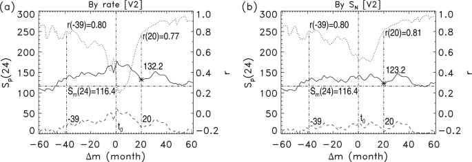

  

  Similar to Figure 6 but using the sunspot numbers of Version 2.0. The horizontal dash-dotted line indicates the maximum amplitude [$S_{\mathrm{m}}(24)=116.4$] of Cycle 24.

• ii) Using the sunspot number at the declining ($\Delta m<0$) and rising ($\Delta m>0$) phase (Figure 7b), the lowest correlation coefficient for Cycles 1 – 23 is $r(\Delta m)=0.51$ at $\Delta m=9$. With the increase of $|\Delta m|$, $r(\Delta m)$ tends to increase and $r(\Delta m)>0.75$ if $\Delta m\leqslant -16$ or $\Delta m\geqslant 18$. The mean prediction error is $\overline{\Delta S}_{\mathrm{p}}= 14.4$ ($\overline{E}_{\mathrm{r}}=12.3 \%$) for $\Delta m>0$ and $\overline{\Delta S}_{\mathrm{p}}= 14.5$ ($\overline{E}_{\mathrm{r}}=12.4\%$) for $\Delta m<0$. At $\Delta m=-39$, $r(-39)=0.80$ and $\Delta S_{\mathrm{p}}=13.2$ ($E_{\mathrm{r}}=11.3\%$). For $\Delta m>0$, the prediction error is minimum (maximum), $\Delta S_{\mathrm{p}}=0.4$ (30.5), at $\Delta m=51$ (31) and has a local minimum [6.4] at $\Delta m=21$. At $\Delta m=20$ (similar to the time for predicting Cycle 25), $r(20)=0.81$, $S_{\mathrm{p}}=123.2$ (asterisk), and $\Delta S_{\mathrm{p}}=6.8$ ($E_{\mathrm{r}}=5.8\%$).

Using the sunspot number (Figure 7b), the correlation coefficient is slightly higher, and the prediction error tends to be smaller than that using either a decrease or rising rate (Figure 7a). Near the solar minimum, the correlation coefficient tends to be weaker, and the prediction error tends to be larger than those at other $\Delta m$. The mean relative prediction error for Cycle 24 using the data of the new version is larger than that using the data from Version 2.0.

References

Burud, D.S., Jain, R., Awasthi, A.K., Chaudhari, S., Tripathy, S.C., Gopalswamy, N., Chamadia, P., Kaushik, S.C., Vhatkar, R.: 2021, Spotless days and geomagnetic index as the predictors of solar cycle 25. Res. Astron. Astrophys. 21, 215. DOI.
Cameron, R., Schüssler, M.: 2007, Solar cycle prediction using precursors and flux transport models. Astrophys. J. 659, 801. DOI.
Cameron, R., Schüssler, M.: 2008, A robust correlation between growth rate and amplitude of solar cycles: consequences for prediction methods. Astrophys. J. 685, 1291. DOI.
Choudhuri, A.R., Chatterjee, P., Jiang, J.: 2007, Predicting solar cycle 24 with a solar dynamo model. Phys. Rev. Lett. 98, 131103. DOI.
Chowdhury, P., Kilcik, A., Yurchyshyn, V., Obridko, V.N., Rozelot, J.P.: 2019, Analysis of the hemispheric sunspot number time series for the solar cycles 18 to 24. Solar Phys. 294, 142. DOI.
Chowdhury, P., Jain, R., Ray, P.C., Burud, D., Chakrabarti, A.: 2021, Prediction of amplitude and timing of solar cycle 25. Solar Phys. 296, 69. DOI.
Clette, F., Cliver, E., Lefèvre, L., Svalgaard, L., Vaquero, J., Leibacher, J.: 2016, Preface to topical issue: recalibration of the sunspot number. Solar Phys. 291, 2479. DOI.
Clette, F., Lefèvre, L.: 2016, The new sunspot number: assembling all corrections. Solar Phys. 291, 2629. DOI.
Dikpati, M., de Toma, G., Gilman, P.A.: 2006, Predicting the strength of solar cycle 24 using a flux-transport dynamo-based tool. Geophys. Res. Lett. 33, L05102. DOI.
Du, Z.L.: 2006, Relationship between solar maximum amplitude and max-max cycle length. Astron. J. 132, 1485. DOI.
Du, Z.L.: 2020a, Predicting the shape of solar cycle 25 using a similar-cycle method. Solar Phys. 295, 134. DOI.
Du, Z.L.: 2020b, Predicting the amplitude of solar cycle 25 using the value 39 months before the solar minimum. Solar Phys. 295, 147. DOI.
Du, Z.L.: 2020c, The solar cycle: predicting the peak of solar cycle 25. Astrophys. Space Sci. 365, 104. DOI.
Du, Z.L.: 2022, The solar cycle: a modified Gaussian function for fitting the shape of the solar cycle and predicting cycle 25. Astrophys. Space Sci. 367, 20. DOI.
Du, Z.L., Du, S.Y.: 2006, The relationship between the amplitude and descending time of a solar acticity cycle. Solar Phys. 238, 431. DOI.
Du, Z.L., Wang, H.N.: 2010, Does a low solar cycle minimum hint at a weak upcoming cycle? Res. Astron. Astrophys. 10, 950. DOI.
Du, Z.L., Wang, H.N.: 2011, The prediction method of similar cycles. Res. Astron. Astrophys. 11, 1482. DOI.
Du, Z.L., Wang, H.N.: 2012, Predicting the solar maximum with the rising rate. Sci. China Ser. G, Phys. Mech. Astron. 55, 365. DOI.
Du, Z.L., Wang, H.N., He, X.T.: 2006, The relation between the amplitude and the period of solar cycles. Chin. J. Astron. Astrophys. 6, 489. DOI.
Gleissberg, W.: 1971, The probable behaviour of sunspot cycle 21. Solar Phys. 21, 240. DOI.
Gnevyshev, M.N., Ohl, A.I.: 1948, On the 22-year cycle of solar activity. Astron. Zh. 25, 18.
Han, Y.B., Yin, Z.Q.: 2019, A decline phase modeling for the prediction of solar cycle 25. Solar Phys. 294, 107. DOI.
Hathaway, D.H.: 2010, The solar cycle. Living Rev. Solar Phys. 7, 1. DOI.
Hathaway, D.H., Upton, L.A.: 2016, Predicting the amplitude and hemispheric asymmetry of solar cycle 25 with surface flux transport. J. Geophys. Res. 121, 10,744. DOI.
Hathaway, D.H., Wilson, R.M., Reichmann, E.J.: 1994, The shape of the sunspot cycle. Solar Phys. 151, 177. DOI.
Hathaway, D.H., Wilson, R.M., Reichmann, E.J.: 1999, A synthesis of solar cycle prediction techniques. J. Geophys. Res. 104, 22375. DOI.
Javaraiah, J.: 2016, North-South asymmetry in small and large sunspot group activity and violation of even-odd solar cycle rule. Astrophys. Space Sci. 361, 208. DOI.
Kakad, B., Kakad, A.: 2021, Forecasting peak smooth sunspot number of solar cycle 25: a method based on even-odd pair of solar cycle. Planet. Space Sci. 209, 105359. DOI.
Kane, R.P.: 2007, A preliminary estimate of the size of the coming solar cycle 24, based on Ohl’s precursor method. Solar Phys. 243, 205. DOI.
Kitiashvili, I.N.: 2021, Effects of observational data shortage on accuracy of global solar activity forecast. Mon. Not. Roy. Astron. Soc. 505, 6085. DOI.
Murphy, A.H., Epstein, E.S.: 1989, Skill scores and correlation coefficient in model verification. Mon. Weather Rev. 117, 572. DOI.
Nandy, D.: 2021, Progress in solar cycle predictions: sunspot cycles 24-25 in perspective. Solar Phys. 296, 54. DOI.
Nordemann, D.J.R., Trivedi, N.B.: 1992, Sunspot number time series – exponential fitting and periodicites. Solar Phys. 142, 411. DOI.
Ohl, A.I., Ohl, G.I.: 1979, A new method of very long-term prediction of solar activity. In: Donnelly, R.F. (ed.): NASA Marshall Space Flight Center Solar-Terr. Pred. Proc. 2 258. ADS.
Pesnell, W.D.: 2012, Solar cycle predictions (invited review). Solar Phys. 281, 507. DOI.
Pesnell, W.D., Schatten, K.H.: 2018, An early prediction of the amplitude of solar cycle 25. Solar Phys. 293, 112. DOI.
Petrovay, K.: 2020, Solar cycle prediction. Living Rev. Solar Phys. 17, 2. DOI.
Ramesh, K.B., Lakshmi, N.B.: 2012, The amplitude of sunspot minimum as a favorable precursor for the prediction of the amplitude of the next solar maximum and the limit of the Waldmeier effect. Solar Phys. 276, 395. DOI.
Sarp, V., Kilcik, A., Yurchyshyn, V., Rozelot, J.P., Ozguc, A.: 2018, Prediction of solar cycle 25: a non-linear approach. Mon. Not. Roy. Astron. Soc. 481, 2981. DOI.
Schatten, K.H.: 2005, Fair space weather for solar cycle 24. Geophys. Res. Lett. 32, L21106. DOI.
Schatten, K., Myers, D.J., Sofia, S.: 1996, Solar activity forecast for solar cycle 23. Geophys. Res. Lett. 23, 605. DOI.
Schatten, K.H., Scherrer, P.H., Svalgaard, L., Wilcox, J.M.: 1978, Using dynamo theory to predict the sunspot number during solar cycle 21. Geophys. Res. Lett. 5, 411. DOI.
Singh, P.R., Tiwari, C.M., Saxena, A.K., Agrawal, S.L.: 2019, Quasi-biennial periodicities and heliospheric modulation of geomagnetic activity during solar cycles 22. Phys. Scr. 94, 105005. DOI.
Singh, P.R., Saad, F.A.I., Singh, A.K., Pant, T.K., Aly, A.A.: 2021, Predicting the maximum sunspot number and the associated geomagnetic activity indices AA and Ap for solar cycle 25. Astrophys. Space Sci. 366, 48. DOI.
Solanki, S.K., Krivova, N.A., Schussler, M., Fligge, M.: 2002, Search for a relationship between solar cycle amplitude and length. Astron. Astrophys. 396, 1029. DOI.
Stewart, J.Q., Panofsky, H.A.A.: 1938, The mathematical characteristics of sunspot variations. Astrophys. J. 88, 385. DOI.
Svalgaard, L., Cliver, E.W., Kamide, Y.: 2005, Sunspot cycle 24: smallest cycle in 100 years? Geophys. Res. Lett. 32, L01104. DOI.
Takalo, J.: 2020, Comparison of latitude distribution and evolution of even and odd sunspot cycles. Solar Phys. 295, 49. DOI.
Thompson, R.J.: 1988, The rise of solar cycle number 22. Solar Phys. 117, 279. DOI.
Thompson, R.J.: 1993, A technique for predicting the amplitude of the solar cycle. Solar Phys. 148, 383. DOI.
Usoskin, I.G., Mursula, K.: 2003, Long-term solar cycle evolution: review of recent developments. Solar Phys. 218, 319. DOI.
Waldmeier, M.: 1939, Über die struktur der sonnenflecken. Astron. Mitt. Zürich 14, 439. ADS.
Wang, J.L., Gong, J.C., Liu, S.Q., Le, G.M., Han, Y.B., Sun, J.L.: 2002, Verification of a similar cycle prediction for the ascending and peak phases of solar cycle 23. Chin. J. Astron. Astrophys. 2, 396. DOI.
Wilson, R.M.: 1990, On the maximum rate of change in sunspot number growth and the size of the sunspot cycle. Solar Phys. 127, 199. DOI.
Yin, Z.Q., Han, Y.B.: 2018, An improved prediction of sunspot maximum by Vondrak smoothing method. Astron. Nachr. 339, 30. DOI.
Yoshida, A.: 2014, Difference between even- and odd-numbered cycles in the predictability of solar activity and prediction of the amplitude of cycle 25. Ann. Geophys. 32, 1035. DOI.
Yoshida, A., Yamagishi, H.: 2010, Predicting amplitude of solar cycle 24 based on a new precursor method. Ann. Geophys. 28, 417. DOI.
Acknowledgments
The author is grateful to the anonymous reviewer for valuable suggestions that improved this manuscript.
Funding
This work was supported by National Key R&D Program of China under grant 2021YFA1600504 and the National Science Foundation of China (NSFC) under grants 11873060 and 11973058.
Author information
Authors and Affiliations
Contributions
The data analysis and the manuscript were completed by DZL.
Corresponding author
Ethics declarations
Conflict of Interest
The author declares that he has no conflicts of interest.
Additional information
Publisher’s Note
Springer Nature remains neutral with regard to jurisdictional claims in published maps and institutional affiliations.