Optimization of Load-Carrying Hierarchical Stiffened Shells: Comparative Survey and Applications of Six Hybrid Heuristic Models

Abstract

The accurate result of heuristic models combined by social inspired optimization methods is interesting issue for optimizations of hierarchical stiffened shells (HSS). In this paper, six heuristic combined by social-inspired optimization is compared for both ability and accuracy in optimization of load-carrying capacities of HSS. A three level optimization method is employed as (1) explicit dynamic method to provide the train database of optimization model, (2) six heuristic models including response surface method (RSM), multivariate adaptive regression splines (MARS), Kriging, artificial neural network, radial basis function neural network (RBFNN), and support vector regression (SVR) for approximating load-carrying capacity of HSS and (3) an improved partial swarm optimization (IPSO) to search for the optimum results of HSS. In IPSO as optimizer operator, a random adjusting process is presented to update the positions of particles using best particle by a dynamical bandwidth generated by normal standard distribution. Optimization performances for accuracy and ability of six heuristic models coupled by IPSO are compared for optimum model as maximum load-carrying capacity under mass constraint of HSS. The SVR, Kriging and RSM combined by IPSO can be introduced as efficient and accurate modeling-based optimization method to evaluate the optimum design of HSS. The best optimal result is obtained by RBFNN while the worst optimum result is given using MARS among other models.

1 Introduction

Stiffened shells are widely implemented for engineering components of launch vehicles and fuselages [1,2,3], which are under axial compression carry load. For improving the ability of stiffened shells against geometric imperfections, Wang et al. [4] proposed innovative hierarchical stiffened shell (HSS) using major and minor stiffeners as larger and smaller sizes. Through the numerical study, Wang et al. [4] pointed out that major failures of HSS are the global buckling, the partial global buckling (happens between major stiffeners), skin local buckling, stiffener local buckling and plastic buckling modes. In comparison to the traditional stiffened shell, the low imperfection sensitivity of HSS was verified by numerical analyses [4,5,6] and experiments [7, 8]. The high load-carrying capacity of HSS was conducted by Wang et al. [9], Tian et al. [10], and Zhao et al. [11]. Particularly, experimental studies were carried out for composite HSS and the load-carrying advantage of HSS was validated [12, 13]. In addition, the abilities of hierarchical stiffened panels against thermal buckling [14] and blast [15] were investigated.

Aiming at improving the load-carrying capacity of HSS, the optimization techniques can be employed for HSS. However, it is two major challenges. First challenge is high buckling analysis cost caused by the complicated stiffener characteristics in the FE analysis of HSS. Tian et al. [16] pointed out that the explicit dynamic method would be more suitable to be used in the optimization process of stiffened shells than other nonlinear buckling methods because it can guarantee the convergence of nonlinear post-buckling analysis. Based on the experimental result, the accuracy and credibility of the explicit dynamic method was validated [17]. However, the computational time of the explicit dynamic method is so heavy that it is hardly used as direct analysis approach in the optimization process. In this case, many efficient analysis models have been proposed. For instance, Wang et al. [18] employed Asymptotic Homogenization Method to smear minor stiffeners of HSS, significantly reducing the post-buckling analysis time of HSS by 84%. Based on Numerical-based Smeared Stiffener Method (NSSM), Wang et al. [9] established an adaptive equivalent strategy for HSS, which can further reduce the post-buckling analysis time of HSS. Sadowski et al. [19] employed a computational strategy to aid researchers in calculating buckling load results of metal shells under various load cases. Although using efficient analysis models, the optimization cost is still too huge. Thus, the surrogate modelling technique has been used to accelerate the optimization efficiency of HSS.

Second challenge is the low accuracy for predictions of optimum HSS using heuristic models. The reason is that the optimization of HSS is a complex optimization problem with multiple design variables. By means of the radial basis function (RBF), Wang et al. [18], Zhao et al. [11] and Hao et al. [20] performed the hybrid optimizations for HSS aiming at maximizing the load-carrying capacity and minimizing the weight. Li et al. [21] applied Kriging-based hybrid aggressive space mapping method for the fast buckling optimization of variable-stiffness cylinders. By considering the limitation of optimization using surrogate model as inaccurate predictions for ultimate conditions of structures, the global optimizing ability is challenged. In order to enhance the global optimizing ability of surrogate-based optimizations of HSS, Tian et al. [22] proposed a competitive sampling method based on multi-fidelity analysis methods. Multi-fidelity surrogate technology has been proposed to improve the abilities for accuracy and computational efficiency of heuristic optimizations [23, 24]. The objective of this paper is to develop more accurate surrogate models for optimizations of HSS. To achieve for this aim, an optimization framework is implemented to compare and to review of six heuristic optimization methods using three levels of (1) explicit dynamic method to provide the train database for calibrating the models, (2) heuristic models to predict the optimization models and (3) improved partial swarm optimization (IPSO) to search the optimal conditions of HSS. Six heuristic approaches as soft computing and statistical models are applied which include the response surface method (RSM), multivariate adaptive regression splines (MARS), Kriging, artificial neural network (ANN), radial basis function neural network (RBFNN), and support vector regression (SVR). As given from comparative results, the IPSO provides the best optimum results compared to PSO while the RBFNN as soft computing model and Kriging as statistical approach are provided the accurate optimal results compared to other models.

2 Analytical Approach-Based FE Analysis

In this paper, the explicit dynamic method is used as the analytical approach of HSS, which can capture the ultimate load-carrying capacity of HSS and has a good agreement with the experiment [17]. The formulation of the explicit dynamic method is as follows,

$${\mathbf{Ma}}_{t} = {\mathbf{F}}_{t}^{ext} - {\mathbf{F}}_{t}^{int} - {\mathbf{CV}}_{t} - {\mathbf{KU}}_{t}$$

(1)

where M stands for the mass matrix, a stands for the vector of nodal acceleration, ${\mathbf{F}}_{t}^{ext}$ stands for the vector of applied external force, ${\mathbf{F}}_{t}^{int}$ stands for the vector of internal force, C stands for the damping matrix, V stands for the vector of nodal velocity, K stands for the stiffness matrix, U stands for the vector of nodal displacement, and t stands for the time. Here, the explicit time integration with the central difference method is employed to approximate velocity and acceleration.

3 Heuristic Data-Driven Approaches

In this section, six modelling approaches to predict the objective performance function as load-carrying capacity and subjective function as mass are presented using mathematical functions by the following relations:

3.1 Response Surface Method (RSM)

The RSM is a simple approximated tool which is commonly defined using second-order polynomial basic functions as below [25, 26]:

$$P(X) = a_{0} + \sum\limits_{i = 1}^{NV} {a_{i} } x_{i} + \sum\limits_{i = 1}^{NV} {\sum\limits_{j = i}^{NV} {a_{ij} } } x_{i}^{{}} x_{j}^{{}}$$

(2)

where $P(X)$ is the predicted objective or subjective conditions for HSS which is predicted using $NV$ number of input variables x including t_s (skin thickness), N_aj (number of axial major stiffeners), N_an (axial minor stiffeners between axial major stiffeners), N_cj (number of circumferential major stiffeners), N_cn (circumferential minor stiffeners between circumferential major stiffeners), h_rj (major stiffener height), h_rn (minor stiffener height), t_rj (major stiffener thickness) and t_rn (minor stiffener thickness). $a_{0,\,} a_{i\,}$ and $a_{ij}$ are unknown coefficients for polynomial terms which are computed using least square estimator [27, 28]:

3.2 Multivariate Adaptive Regression Spline (MARS)

The MARS is a statistical regression tool as nonlinear and nonparametric technique presented by Friedman [29]. The MARS can be used to simulate the nonlinear relations between structural response as predicted function and the input variables by piecewise linear splines basis function (BF) as below form:

$$P(\varvec{X}) = \beta_{0} + \sum\limits_{i = 1}^{m} {\beta_{i} } BF_{i}$$

(3)

where $\beta_{i}$ = 0, 1, …, m are unknown coefficients and m is the number basis functions ($BF$) that it is given using forward backward stepwise scheme. $BF_{i}$ is computed from piecewise linear function as follows:

$$BFi = \{ \hbox{max} (0,x - C_{i} )\,,\,\hbox{max} (0,C_{i} - x)\}$$

(4)

In which, C is knot which is a constant coefficient. The applied basis functions ($BF$) are explored by using a stepwise process. The model using MARS is structured by using two stages as (i) BF functions and their potential knots are chosen to provide the accurate prediction in first stage, and (ii) in second stage, the BF terms with lowest effect are eliminated [30].

3.3 Kriging Method

The Kriging model is a well-known framework to estimate the geostatistical problems [31]. The Kriging model is presented as follows [32]:

$$P(X) = G(X)^{T} \beta + r(X)^{T} \gamma$$

(5)

where G(X) the basic functions. β is unknown coefficient vector which is computed as:

$$\beta = (G^{T} R^{ - 1} G)^{ - 1} G^{T} R^{ - 1} O$$

(6)

where O represents the observed load and mass of shell. R denotes the correlation as

$$R = \left[ {\begin{array}{*{20}c} 1 & {} & {r(\mathop X\nolimits_{1} ,\mathop X\nolimits_{2} )} & \ldots \\ {r(\mathop X\nolimits_{2} ,\mathop X\nolimits_{1} )} & {} & 1 & {} \\ {} & \vdots & {} & \ddots \\ {r(\mathop X\nolimits_{n} ,\mathop X\nolimits_{1} )} & {} & {r(\mathop X\nolimits_{n} ,\mathop X\nolimits_{1} )} & \cdots \\ \end{array} \begin{array}{*{20}c} {r(\mathop X\nolimits_{1} ,\mathop X\nolimits_{n} )} \\ {r(\mathop X\nolimits_{2} ,\mathop X\nolimits_{n} )} \\ \vdots \\ 1 \\ \end{array} } \right]$$

(7)

In which, r (X_i, X_j) is the covariance basis function which is given as follows:

$$r\left( {\mathop X\nolimits_{i} ,\mathop X\nolimits_{j} } \right) = \mathop e\nolimits^{{\theta \mathop r\nolimits_{ij}^{2} }}$$

(8)

where θ is unknown correlation parameters θ ˃ 0 and $r_{ij} = \left\| {X_{i} - X_{j} } \right\|$. In Eq. (5), $r(X) = [R(X_{1} ,X;\theta ),R(X_{2} ,X;\theta ), \ldots ,R(X_{n} ,X;\theta )]^{T}$ and $\gamma = R^{ - 1} (O - G^{T} \beta )$ [28]. It can be conducted from Kriging model that the predicted data is computed using a covariance terms by using the correlation matrix $R$ which it may provide the nonlinear relation for a complex engineering problem.

3.4 Support Vector Regressions (SVR)

The support vector machines-based learning approaches are a powerful intelligent approach to regress the nonlinear problems [33]. For a N-set database, the SVR basis predicted function is presented as below:

$$P(\varvec{X}) = \beta_{0} + \sum\limits_{i = 1}^{N} {(\alpha_{i} - \alpha_{i}^{*} )} K(\varvec{x},\varvec{x}_{i} )$$

(9)

where $\beta_{0}$ is bias and $K(\varvec{x},\varvec{x}_{i} )$ is the Kernel function for transferring the input data from x- space to N-set feature space. The Gaussian radial basis function as kernel functions is used in this current study as below relation [34, 26]:

$$K(\varvec{x},\varvec{x}_{i} ) = \exp \left( { - \frac{{\left\| {\varvec{x} - \varvec{x}_{i} } \right\|^{2} }}{{2\sigma^{2} }}} \right)$$

(10)

where $\sigma$ is the parameter of Kernel function. In Eq. (9), $\alpha_{i}^{{}}$ and $\alpha_{i}^{*}$ represent the Lagrange multipliers which is determined based on maximizing the regression function as below [35]:

$$\begin{aligned} & Maximize\quad - \frac{1}{2}\sum\limits_{i,j = 1}^{N} {(\alpha_{i} - \alpha_{i}^{*} )(\alpha_{j} - \alpha_{j}^{*} )} K(\varvec{x}_{i} ,\varvec{x}_{j} ) - \varepsilon \sum\limits_{i = 1}^{N} {(\alpha_{i} - \alpha_{i}^{*} ) + } \sum\limits_{i = 1}^{N} {y_{i} (\alpha_{i} - \alpha_{i}^{*} )} \\ & Subjected\,to\,\left\{ {\begin{array}{*{20}l} {\sum\limits_{i = 1}^{N} {(\alpha_{i} - \alpha_{i}^{*} ) = 0} } \hfill \\ {0 \le \alpha_{i} \le C} \hfill \\ {0 \le \alpha_{i}^{*} \le C} \hfill \\ \end{array} } \right. \\ \end{aligned}$$

(11)

where ε-insensitive loss function is used for neglecting values of predicted data less than the observed values in regression process. Factor C > 0 represent the regularization coefficient. The accuracy of the predicted SVR model can be improved by perfect selection of the model parameters as $\sigma$, $\varepsilon$ and C. In this work, the parameters of SVR models are selected by trial and error.

3.5 Artificial Neural Network (ANN)

Artificial neural network (ANN) model is a well-Known popular learning process to provide the nonlinear relation between input set and output observation. The multilayer feed forward neural network is commonly applied in ANN models, which is presented by the following relation [36]:

$$P(X) = \left[ {\mathop \beta \nolimits_{0} + \sum\limits_{j = 1}^{M} {\mathop w\nolimits_{j} } f_{1} \left( {\beta_{j} + \sum\limits_{i = 1}^{NV} {\mathop w\nolimits_{ij} } x_{i} } \right)} \right]$$

(12)

where β₀ and $\beta_{j}$ are respectively the biases for output data and M-hidden layer, w_ij denotes the weights to joint j-th input variable and j-th hidden neuron while w_j represent the weights of output neuron which provide the relations between j-th hidden neuron and output data, f is an activation function for hidden neurons. The active function f is given as sigmoid function by following relation:

$$f\left( X \right) = \frac{1}{1 + \exp ( - X)}$$

(13)

The ANN model is structured using NV input variable (i.e. NV = 9 in this current study) and M hidden neurons that it is selected between 5 and 25 by using trial and error for both load and mass models in this study. The back-propagation is a most common learning approach to calibrate the ANN in Eq. (12) which is applied to search the weights and biases. The Levenberg–Marquardt back-propagation method [37] is utilized for normalized input and output data sets between − 1 and 1, in this study.

3.6 Radial Basis Function Neural Network (RBFNN)

The RBFNN can be provided the efficient and accurate prediction compared to the ANN-based multilayer feed forward for some nonlinear problems due to fast training process and simple structure [38, 39]. The mathematical relation-based radial basis function (RBF) is presented as below:

$$P(X) = \mathop \beta \nolimits_{0} + \sum\limits_{j = 1}^{M} {\mathop w\nolimits_{j} } \varphi (||x - C_{i} ||)$$

(14)

where $\mathop w\nolimits_{j}$ represents the weights to link j-th hidden neuron (j = 1, …, M) and output data while, Cj is the center j-th RBF of hidden neuron. $\phi$ refers to activation function which is defined using Gaussian function as follows:

$$\varphi (||x - C_{i} ||) = \exp \left( { - \frac{{||x - C_{i} ||^{2} }}{{\sigma_{i}^{2} }}} \right)$$

(15)

$\sigma$ is the RBF parameter. The RBFNN involves three basic layers including input, hidden layer and output layers. The input layer contains NV neurons. The hidden layer involves of M RBFs which transform the NV dataset to M-dimensional input database.

4 Optimization Schemes

Two optimization approaches using the partial swarm optimization (PSO) are utilized to find the optimal conditions of HSS in this current study. The original PSO and a proposed improved PSO (IPSO) is presented as below subsections.

4.1 PSO Scheme

The particle swarms as social psychologist can be used as an optimization process to find the best manner of the engineering problems. The PSO is a computational intelligence by using a simple formulation and high-abilities in optimization problems. This approach is extracted from the psychological behavior of birds for searching the corn as food that this behavior of animals is applied into an optimization method as Particle Swarm Optimization (PSO) [40]. In PSO, the pattern of each particle (bird) is random simple perturbations to search optimum conditions (food) that the position of each particle is computed using the current position of particles, best particle among current position and the best position among the history of their movements as below relations:

$$\begin{aligned} & \varvec{V}_{k + 1} = \omega_{k} \varvec{V}_{k} + c_{1} r_{1} [p_{best} - \varvec{X}_{k} ] + c_{2} r_{2} [g_{best} - \varvec{X}_{k} ] \\ & \varvec{X}_{k + 1}^{{}} = \varvec{X}_{k} + \varvec{V}_{k + 1} \\ \end{aligned}$$

(16)

In which, $g_{best}$ and $p_{best}$ are respectively the best population of each partial and best population in current positions. c₁ and c₂ are acceleration coefficients which set as 2 and r₁ and r₂ are two random uniform numbers in the range from 0 to 1. $\omega_{k}$ is inertia weight which is computed as follows:

$$\omega_{k} = \omega_{\hbox{min} } + \frac{NI - k}{NI}(\omega_{\hbox{max} } - \omega_{\hbox{min} } ),\,\,$$

(17)

where $\omega_{\hbox{min} }$ = 0.4 and $\omega_{\hbox{max} } = 0.9$. In PSO process, maximum ($v_{{}}^{\hbox{max} }$) and minimum ($v_{{}}^{\hbox{min} }$) velocities are respectively given as $\frac{{x_{{}}^{U} - x_{{}}^{L} }}{10}$ and $- \frac{{x_{{}}^{U} - x_{{}}^{L} }}{10}$ ($x_{{}}^{U}$ and $x_{{}}^{L}$ are the variables upper and lower bound for x) that the initial each particle velocity is randomly computed in the domain of $v_{{}}^{\hbox{max} }$ and $v_{{}}^{\hbox{min} }$.

4.2 Improved PSO Scheme (IPSO)

The convergence speed rate and global optimal results are two major important characteristics of efforts to apply the optimization methods as PSO. It can be used a variant of IPSO algorithm to achieve the best performances for both fast convergence and avoiding the local optima than PSO. Consequently, the ability of PSO is enhanced using random adjusting sachem for optimizing load-carrying capacity of HSS. This methodology randomly involves two major adapting proposes for each particle as well as PSO in first sage and the best conditions in second stage. In second adjusting step, the best population is adjusted based on a random pitch-adjusting normal term as follows:

$$\varvec{X}_{k + 1}^{{}} = g_{best} + Normrand(0,1) \times \sqrt {1 - \frac{k}{NI}}$$

(18)

where k and NI are respectively the current and total iterations. Based on Eq. (18), the best particles $g_{best}$ are adjusted by using a normal random value with mean of 0 and stranded deviation of 1 ($Normrand(0,1)$). The factor $\sqrt {1 - \frac{k}{NI}}$ in Eq. (5) gives larger values at the initial iterations while computes the smaller values at the final iteration. It is assumed, the new positions are randomly adjusted using the best population and the PSO adjusting process. Therefore, Eqs. (17) and (18) are randomly combined to adopt the new position in IPSO as below:

$$\varvec{X}_{k + 1}^{{}} = \left\{ {\begin{array}{*{20}l} {\varvec{X}_{k} + \varvec{V}_{k + 1} } \hfill &\quad {r < 0.8 - 0.4\frac{k}{NI}} \hfill \\ {g_{best} + Normrand(0,1) \times \sqrt {1 - \frac{k}{NI}} } \hfill &\quad {otherwise} \hfill \\ \end{array} } \right.$$

(19)

where $\varvec{V}_{k + 1}$ is computed using Eq. (16) and r is a random = number in the range from 0 to 1.

5 Hierarchical Stiffened Shell (HSS)

5.1 Studied Example of HSS

The configuration of HSS is displayed in Fig. 1. The diameter D of the HSS is 3000 mm, and the length L of the HSS is 2000 mm. The HSS has 9 design variables, including N_aj, N_cj, N_an, N_cn, t_s, h_rj, h_rn, t_rj, and t_rn. The design space of 9 design variables is listed in Table 1. The material of the HSS is SiC particle reinforced Al matrix (SiC/Al) composites, which is a potential composite material used in aerospace fields [41]. The mechanical properties of SiC/Al composites are as follows: Young’s modulus E = 100,000 MPa and Poisson’s ratio υ = 0.3. The boundary condition of the HSS is to keep the lower end of the HSS clamped and the upper end fixed except the degrees of freedom along the axial direction. A uniform axial load is applied to the upper end of the HSS.

Fig. 1

Schematic diagram of hierarchical stiffened shell

Table 1 The design space of design variables for hierarchical stiffened shell

5.2 Database of HSS

The data of HSS for evaluating load-carrying capacity under mass constraint in the modeling process are computed using the FE method. The input data sets in train and test phases of nine variables of HSS are simulated using the Latin hypercube sampling (LHS) that these input data sets in train and test are jointed to a computer program to compute the load capacity and mass of HSS. The total data of train and test data are respectively given as 430 and 100 data points that the statistical properties of data including maximum (X_max), minimum (X_min), average (Xmean), standard deviations (STD) and coefficient of variations (COV) for test and train datasets are presented in Table 2. Four input (i.e. N_aj, N_an, N_cj and N_cn) data are integer while other are continues variables. The COVs of input variables are varied in the range from 0.2 to 0.4 in training period and from 0.15 to 0.4 in testing period. The different of COVs between test and train data are shown in load data obtained by FE model. The bar diagram of the train and test data computed by FE analysis for studied problem are presented in Figs. 2 and 3, respectively. As seen, the load capacities in train and test phases are respectively varied about 15,000–24,000 kN and 11,000–19,000 kN while the mass effective domains are respectively computed as 265–465 kg and 245–395 kg for train and test databases.

Table 2 statistical properties of input data and FE results of load and mass in train and test phases

Fig. 2

Bar diagram of evaluated FE analysis for load capacity and mass in training data pints

Fig. 3

Bar diagram of evaluated FE analysis for load capacity and mass in testing data pints

6 Simulation and Optimization Results

The results based on three-level optimization process involve two major categories. In the first category, the predicted results in test phase based on the six studied models are presented. The models-based mechanical learning approach are trained by the parameters which are determined using trial and error as (1) the parameters of SVR are C = 9000, σ = 16.5 and ε = 0.25 for training load and C = 5000, σ = 15 and ε = 0.15 for training mass, (2) the hidden layers in training process-based ANN are M = 11 for load and M = 23 for mass while (3) the parameters of RBFNN models are M = 95 and σ = 0.5 for load and M = 83 and σ = 2.5 for mass. The calibrating models using six heuristic data-driven approaches including RSM, Kriging, MARS, SVR, ANN and RBFNN are used in optimization process-based PSO and IPSO that the optimization results are compared in second category.

6.1 Comparative Results for Modelling Conditions of HSS

The model’s accuracy was evaluated using statistical comparative factors including root mean square error (RMSE), mean absolute error (MAE), Nash and Sutcliffe efficiency (NES) and modified agreement index (d) statistics as below:

$$MAE = \frac{1}{N}\sum\limits_{i = 1}^{N} {|O_{i} - P_{i} |}$$

(20)

$$RMSE = \sqrt {\frac{1}{N}\sum\limits_{i = 1}^{N} {[O_{i} - P_{i} ]^{2} } }$$

(21)

$$d = 1 - \frac{{\sum\nolimits_{i = 1}^{N} {|O_{i} - P_{i} |}}}{{\sum\nolimits_{i = 1}^{N} {(|O_{i} - \overline{O}_{{}} | + |P_{i} - \overline{O} |)}}},\quad 0 < d \le 1$$

(22)

$$NES = 1 - \frac{{\sum\nolimits_{i = 1}^{N} {|O_{i} - P_{i} |}}}{{\sum\nolimits_{i = 1}^{N} {|O_{i} - \overline{O} |}}},\quad - \infty < NES \le 1$$

(23)

where N is the number of data in training phase (430) and testing phase (100), O, $P$ and $\overline{O}$ are the observed FE, predicted models and mean of observed FE for mass or load-carrying capacity force, respectively. The comparative statistics of different predicted data-driven models for test (validation) dataset are presented in Table 3. The observed data computed by FE method corresponding to predicted data points approximated by studied models are plotted in Figs. 4 and 5 for load and mass in test phase, respectively.

Table 3 Comparative statistics of different models in test phases

Fig. 4

Scatterplot for FE model-based computed data and models-based predicted data of load in test phase

Fig. 5

Scatterplot for FE model-based computed data and models-based predicted data of mass in test phase

By presented results in Table 3 and Fig. 4 for load database, the accurate prediction is determined using the RSM and Kriging models by comparing the NSE and d which are also followed by the machine learning approaches as ANN, SVR and RBFNN models, while the MARS is ranked at the last predicted model for evaluating the load capacity of HSS. According to R² in Fig. 4, the ANN model shows the highest R² (R² = 0.8709) which follows by Kriging (R² = 0.8689) and RBFNN (R² = 0.8662) models while the lowest R² is 0.8518 which obtained by MARS model. Finally, the Kriging model has the highest d and NSE (d = 0.625, NSE = 0.238) and the lowest RMSE (RMSE = 3317.6kN) that this modelling approach can be ranked as best among other studied models. The MARS model provides the last lowest RMSE and MAE for load predictions. Corresponding to RMSE values, the ranked models for predicting load are Kriging, RMS, ANN, SVR, RBFNN and MARS.

The results in Table 3 and Fig. 5 for mass indicated that the RBFNN method guaranteed highly accuracy for prediction of mass by comparing the statistics of NSE = 0.774, d = 0.889 and MAE = 12.416 kg. By applying nine input data, the all models can be provided the accurate predictions with high-correlation for mass while the predicted results for load are shown the inaccurate results. By comparing NSE values, the Kriging is followed the results as well as ANN while the RSM, and MARS models are ranked in second level. The worst method is ANN (NSE = 0.769) compared to other models. As seen, the Kriging, RBFNN, RSM and SVR performed the better than other models for predictions of mass with high-accuracy. It is evaluated the accuracy of models by RMSE (Table 3) and R² (Fig. 5) that the best accuracy is obtained using RBFNN and SVR models. However, the MARS and ANN is decreased the accuracy of mass predictions. Finally, the RBFNN has the highest estimated accuracy (R² = 0.9998), while the MARS has the lowest accuracy (R² = 0.9885) for mass evaluation as constraint function of the optimization HSS model. The best models for prediction of mass are not confirmed the same models which are provided the best predictions for load. Consequently, the models for approximate the optimization model as well as the optimization process are importance to compute the accurate optimal results of HSS. The approximated results of different models to simulate the load as objective and mass as subjective functions are important issues in optimization process.

6.2 Comparative Results

The optimization process is included two subsections as i) evaluating the performances of PSO and IPSO for both fast convergence rate and avoiding the local optimum ii) evaluating the accuracy of optimum conditions.

6.2.1 Comparison of PSO and IPSO

The optimization method of PSO and IPSO are used with a same optimization factors as number of total iterations = 4000, number of particles = 20, c₁ = c₂ = 2, $\omega_{\hbox{min} }$ = 0.4 and $\omega_{\hbox{max} } = 0.9$. The initial particles for all design variables are randomly generated in the range from maximum and minimum values presented in Table 1 as design domains while the initial velocities of particles are given in the range from $\frac{{x_{{}}^{U} - x_{{}}^{L} }}{10}$ to $- \frac{{x_{{}}^{U} - x_{{}}^{L} }}{10}$. The different models are applied to simulate the load as objective and mass as subjective and then the PSO and IPSO are implemented to search optimal design point of HSS. The optimization results of different modelling approaches for both PSO and IPSO are computed. The results of optimization methods in terms of various six models are compared based on 5-run time which are separately computed.

The iterative histories of load capacity with respect to the best (maximum) and average of five optimums resulted from optimization method (mean) for PSO and IPSO-based different models are presented in Fig. 6, while the statistical properties of optimum results for five separated runs for optimization method is listed in Table 4 for different models. As seen from result presented in Fig. 6, almost results with respect to mean load are closely followed with best results obtained by IPSO while it is demonstrated the significant differences between the mean and best results of PSO for all models. The proposed IPSO provides the optimum results in almost its run time compared to PSO for all modeling approaches. The IPSO is performed best optimum results compared to the PSO for almost models as RSM, Kriging, ANN and RBFNN models.

Fig. 6

Iterative results of load for different models corresponding to PSO and IPSO

Table 4 Comparison of the statistical optimum results for different models in PSO and IPSO

By comparing the results of Table 4, the STD of IPSO for five runs is obtained less than the relative STD of models computed by PSO that it improved from 41.7 to 14.95 for RBFNN, from 639.42 to 83.15 for ANN, from 656.43 to 80.51 for Kriging and from 224.08 to 4.84 for RSM. This mean that the almost optimum results of IPSO are tended to the best results while PSO may be avoided these conditions for several runs. The obtained results of optimization method indicated that the IPSO can be provided the optimal results compared to PSO while the convergence rate of PSO is strongly improved for all modelling approaches. As seen the modelling method can be affected on the optimum results of HSS as well as PSO and IPSO. The optimum loads using SVR, ANN and MARS models are computed more than 24,000 kN while the optimum loads for RSM and RBFNN are obtained less than 23,500 kN.

6.2.2 Accuracy of Predicted Optimum Results

The accuracies of approximated optimal results for different models are compared in this section. Five optimum results which are obtained using the PSO and IPSO for different modelling approaches are used to compute the mass and load-carrying capacity by FE model. Based on the results computed by FE model corresponding to the optimal design point by modelling approaches, the accuracy models are compared in PSO and IPSO. The design points obtained by PSO and IPSO are applied to compute the load and mass based on FE models whose statistical characteristics as maximum (max), minimum (min), mean and standard deviations (STD) of FE models are presented in Table 5. By comparing results from Tables 4 and 5, the means of leads for FE method and optimization approaches are significantly changed for load predictions using MARS model thus the results obtained by this model cannot cover the appropriate predictions for both load and mass in the optimization process.

Table 5 Comparison of the statistical optimum results using FE method for optimal design points of different models obtained by PSO and IPSO

According to the results obtained by modelling approaches and FE method for mass and load, the errors as |X_FE − X_model|/X_FE × 100 are presented in Tables 6 and 7 for load and mass, respectively. By comparing errors of estimating maximum load presented in Table 5, the best results for the modelling approaches are provided as RBFNN with minimum of 0.08% in PSO and 0.01% in IPSO as first ranked model and SVR with minimum of 0.19% in PSO and 0.03% in IPSO as second ranked model. However, ANN model can be provide the best results for searching optimum conditions while this modeling method to predict load capacity has highest rank but approximated mass by ANN model is also affected on the optimization method and it may provide an optimal design point by ANN model for load with high-error. For mass errors, the best results are obtained using the modelling approaches of RBFNN (min = 0.02 in PSO and min = 1.41 in IPSO), RSM (min = 0.8 in PSO and min = 2.69 in IPSO) and ANN (min = 1.09 in PSO and min = 1.14 in IPSO) while the worst models are as MARS (min = 13.99 in PSO and min = 22.71 in IPSO) and SVR (min = 5.32 in PSO and min = 3.68 in IPSO).

Table 6 Statistical properties of errors between FE method and models for approximated load in PSO and IPSO

Table 7 Statistical properties of errors between FE method and models for approximated mass in PSO and IPSO

The results form Tables 6 and 7 demonstrated that the studied models may affected with different accuracy for modelling load and mass as well as the ANN that it provides the acceptable results for mass while its predictions shows the larger error than other models in load. The predictions results by comparing the train and test data sets can be provided an appropriate way to select a robust model for existing dataset, but the accuracy predictions of the modelling approaches combined by the optimization approaches can not guaranteed. As seen, the RBFNN combined by IPSO can provide the acceptable results for optimization of this problem while the MARS shows the worst prediction for optimization of HSS. This problem as a complex engineering optimization example can be applied for testing other modelling approaches or hybrid intelligent optimization methods, in future.

The best optimal results obtained using PSO and IPSO in terms of accuracy are listed in Table 8 for different models. These results obtained for five runs for both PSO and IPSO which are given based on the minimum errors for approximated load and mass using the proposed optimization approach. The approximated load using IPSO is obtained more the PSO while it is provided the larger mass than the PSO. The approximated modelling approaches can be categorized as three levels for optimization of studied HSS example

Table 8 Optimal results for different models in PSO and IPSO

• 1. The best modelling approaches as RBFNN (P_cr = 23,048.87 in PSO and P_cr = 23,483.08 in IPSO), Kriging (P_cr = 23,450.76 in PSO), and RSM (P_cr = 23,375.43 in PSO) that their buckling modes are shown in Fig. 7. It is conducted that the maximum load-carrying capacity is obtained by RBFNN model combined by IPSO with minimum error. It can be found from Fig. 7 that, buckling modes of optimal results based on RBFNN, Kriging and RSM are elastic buckling modes. Specifically, they are all global buckling modes, which are considered as buckling modes with high load-carrying capacity for HSS [9].

  Fig. 7

  

  Buckling modes of optimal results based on RBFNN, Kriging and RSM

• 2. The accurate extracted optimization results are P_cr = 23,048.87kN, mass = 369.09 kg with optimal design variables as h_j= 29.945 mm, h_n= 15 mm, N_aj= 48, N_an= 4, N_cj= 4, N_cn= 1, t_j= 4.8 mm, t_n= 3.0 mm and t_s= 4.899 mm while the maximum load capacity based on mass less than 375 kg among all models are obtained as P_cr = 23,483.08kN and mass = 374.29 kg with optimal design variables as h_j= 30 mm, h_n= 15 mm, N_aj= 50, N_an= 1, N_cj= 3, N_cn= 1, t_j= 5.75 mm, t_n= 3.0 mm and t_s= 5.529 mm.

• 3. Models with the moderately results as Kriging combined by IPSO, RSM combined by IPSO, SVR combined by both PSO and IPSO and hybrid ANN by PSO and IPSO. As seen, the SVR can be predicted the accurate load but it is required to improve for tuning its parameters for approximating the accurate prediction of mass. On the other hand, the ANN can be provided the robust prediction to modelling mass but its modeling to approximate load shows the huge errors.

• 4. The worst model which provided optimal results with large values of errors is the MARS combined by IPSO and PSO. This non- parametric approach may be loosed its accuracy in approximating the optimal results of this problem that the buckling mode shape of these modelling methods is presented in Fig. 8. It can be observed that, buckling occurs near the boundary of the HSS. According to Ref. [42], this kind of elephant foot mode is referred to as the plastic buckling mode, which is caused by the material yield.

  Fig. 8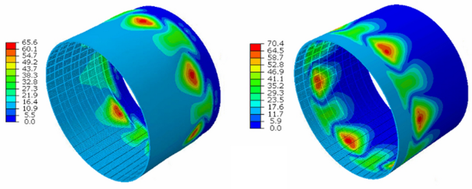

  

  Buckling modes of optimal results based on MARS

7 Conclusion

The optimization process using finite element model is more computationally for evaluating the optimal design-based maximizing load capacity of hierarchical stiffened shells (HSS). Therefore, the hybrid heuristic models can be applied to reduce the computational burden in optimization process. The accuracy of hybrid heuristic models is a major challenge in intelligent optimization approach. In this current work, six heuristic-basis social inspired optimization is reviewed using three-phase framework as follows: i) finite element model to analyze HSS for providing the train and test databases ii) the modelling methodology to approximate the load and mass of optimization model iii) the optimization process to search the optimal design. The main effort of this optimization propos is comparative survey for accuracy of six heuristic approaches including response surface method (RSM), multivariate adaptive regression splines (MARS), Kriging, artificial neural network (ANN), radial basis function neural network (RBFNN), and support vector regression (SVR). Improved partial swarm optimization (IPSO) is presented using random improvisation using the best partial, dynamical bandwidth and normal standard distribution. Based on the comparative results of hybrid models, the following conclusions are extracted.

• 1. The all hybrid heuristic methodan be used for optimization of HSS However, the accuracy of optimal condition is depended on the accurate predictions of data-driven techniques.

• 2. The IPSO provides the superior optimal performances for HSS compared to PSO.

• 3. The best and worst modeling methodologies are RBFNN and MARS among other, respectively. The RSM and Kriging combined by IPSO and PSO can be provided an accurate result compared to SVR combined by IPSO.

• 4. Kriging and RSM combined by IPSO, SVR and ANN combined by PSO and IPSO are shown the lowest accuracy than Kriging and RSM combined by PSO and RBFNN combined by PSO and IPSO.

References

Wagner H, Hühne C, Niemann S, Tian K, Wang B, Hao P (2018) Robust knockdown factors for the design of cylindrical shells under axial compression: analysis and modeling of stiffened and unstiffened cylinders. Thin Walled Struct 127:629–645
Wang D, Abdalla MM, Zhang W (2018) Sensitivity analysis for optimization design of non-uniform curved grid-stiffened composite (NCGC) structures. Compos Struct 193:224–236
Wang D, Abdalla MM, Wang ZP, Su Z (2019) Streamline stiffener path optimization (SSPO) for embedded stiffener layout design of non-uniform curved grid-stiffened composite (NCGC) structures. Comput Method Appl Mech 344:1021–1050
Wang B, Hao P, Li G, Zhang JX, Du KF, Tian K et al (2014) Optimum design of hierarchical stiffened shells for low imperfection sensitivity. Acta Mech Sin 30(3):391–402
Sim CH, Park JS, Kim HI, Lee YL, Lee K (2018) Postbuckling analyses and derivations of knockdown factors for hybrid-grid stiffened cylinders. Aerosp Sci Technol 82–83:20–31
Sim CH, Kim HI, Lee YL, Park JS, Lee K (2018) Derivations of knockdown factors for cylindrical structures considering different initial imperfection models and thickness ratios. Int J Aeronaut Space 19(3):626–635
Quinn D, Murphy A, McEwan W, Lemaitre F (2009) Stiffened panel stability behaviour and performance gains with plate prismatic sub-stiffening. Thin Walled Struct 47(12):1457–1468
Quinn D, Murphy A, McEwan W, Lemaitre F (2010) Non-prismatic sub-stiffening for stiffened panel plates-stability behaviour and performance gains. Thin Walled Struct 48(6):401–413
Wang B, Tian K, Zhao HX, Hao P, Zhu TY, Zhang K et al (2017) Multilevel optimization framework for hierarchical stiffened shells accelerated by adaptive equivalent strategy. Appl Compos Mater 24(3):575–592
Tian K, Zhang JX, Ma XT et al (2019) Buckling surrogate-based optimization framework for hierarchical stiffened composite shells by enhanced variance reduction method. J Reinf Plast Compos 38(21-22):959–973
Zhao YN, Chen M, Yang F, Zhang L, Fang DN (2017) Optimal design of hierarchical grid-stiffened cylindrical shell structures based on linear buckling and nonlinear collapse analyses. Thin Walled Struct 119:315–323
Li M, Sun F, Lai C, Fan H, Ji B, Zhang X et al (2018) Fabrication and testing of composite hierarchical isogrid stiffened cylinder. Compos Sci Technol 157:152–159
Wu H, Lai C, Sun F, Li M, Ji B, Wei W et al (2018) Carbon fiber reinforced hierarchical orthogrid stiffened cylinder: fabrication and testing. Acta Astronaut 145:268–274
Wang C, Xu Y, Du J (2016) Study on the thermal buckling and post-buckling of metallic sub-stiffening structure and its optimization. Mater Struct 49(11):4867–4879
Zhang B, Chen H, Zhao Z, Fan H, Jin F (2018) Blast response of hierarchical anisogrid stiffened composite panel: considering the damping effect. Int J Mech Sci 140:250–259
Tian K, Wang B, Hao P, Waas AM (2018) A high-fidelity approximate model for determining lower-bound buckling loads for stiffened shells. Int J Solids Struct 148:14–23
Wang B, Du K, Hao P, Zhou C, Tian K, Xu S et al (2016) Numerically and experimentally predicted knockdown factors for stiffened shells under axial compression. Thin Walled Struct 109:13–24
Wang B, Tian K, Zhou CH, Hao P, Zheng YB, Ma YL, Wang JB (2017) Grid-pattern optimization framework of novel hierarchical stiffened shells allowing for imperfection sensitivity. Aerosp Sci Technol 62:114–121
Sadowski AJ, Fajuyitan OK, Wang J (2017) A computational strategy to establish algebraic parameters for the reference resistance design of metal shell structures. Adv Eng Softw 109:15–30
Hao P, Wang B, Li G, Meng Z, Tian K, Tang X (2014) Hybrid optimization of hierarchical stiffened shells based on smeared stiffener method and finite element method. Thin Walled Struct 82:46–54
Li E (2017) Fast cylinder variable-stiffness design by using Kriging-based hybrid aggressive space mapping method. Adv Eng Softw 114:215–226
Tian K, Wang B, Zhang K et al (2018) Tailoring the optimal load-carrying efficiency of hierarchical stiffened shells by competitive sampling. Thin Walled Struct 133:216–225
Xu Z, Lu X, Law KH (2016) A computational framework for regional seismic simulation of buildings with multiple fidelity models. Adv Eng Softw 99:100–110
Zhou Q, Yang Y, Jiang P, Shao X, Cao L, Hu J, Gao Z, Wang C (2017) A multi-fidelity information fusion metamodeling assisted laser beam welding process parameter optimization approach. Adv Eng Softw 110:85–97
Khuri AI, Mukhopadhyay S (2010) Response surface methodology. Wiley Interdiscip Rev Comput Stat 2(2):128–149
Gao L , Xiao M, Shao X, Jiang P , Nie L, Qiu H, (2012) Analysis of gene expression programming for approximation in engineering design. Struct Multidiscip Optim 46(3):399–413
Keshtegar B, Heddam S (2018) Modeling daily dissolved oxygen concentration using modified response surface method and artificial neural network: a comparative study. Neural Comput Appl 30(10):2995–3006
Zhang J, Xiao M, Gao L, Chu S, (2019) A combined projection-outline-based active learning Kriging and adaptive importance sampling method for hybrid reliability analysis with small failure probabilities. Computer Methods in Applied Mechanics and Engineering 344:13–33
Friedman JH (1991) Multivariate adaptive regression splines. Ann Stat 19(1):1–67
Zhang WG, Goh ATC (2013) Multivariate adaptive regression splines for analysis of geotechnical engineering systems. Comput Geotech 48:82–95
Oliver MA, Webster R (1990) Kriging: a method of interpolation for geographical information systems. Int J Geogr Inf Syst 4(3):313–332
Zhang Y, Gao L, Xiao M (2020) Maximizing natural frequencies of inhomogeneous cellular structures by Kriging-assisted multiscale topology optimization. Comput Struct 230:106197
Hsu CW, Lin CJ (2002) A comparison of methods for multiclass support vector machines. IEEE Trans Neural Netw 13(2):415–425
Xiao M, Zhang J, Gao L (2020) A system active learning Kriging method for system reliability-based design optimization with a multiple response model. Reliab Eng Syst Safety 199:106935
Basak D, Pal S, Patranabis DC (2007) Support vector regression. Neural Inf Process Lett Rev 11(10):203–224
Hornik K, Stinchcombe M, White H (1989) Multilayer feedforward networks are universal approximators. Neural Netw 2(5):359–366
Sapna S, Tamilarasi A, Kumar MP (2012) Backpropagation learning algorithm based on Levenberg Marquardt Algorithm. Comput Sci Inf Technol: CSIT 2:393–398
Du H, Zhang N (2008) Time series prediction using evolving radial basis function networks with new encoding scheme. Neurocomputing 71(7–9):1388–1400
Chen S, Cowan CFN, Grant PM (1991) Orthogonal least squares learning algorithm for radial basis function networks. IEEE Trans Neural Netw 2(2):302–309
Kennedy J (2010) Particle swarm optimization. In: Sammut C, Webb G (eds) Encyclopedia of machine learning. Springer, Boston, pp 760–766
Cui Y, Wang LF, Ren JY (2008) Multi-functional SiC/Al composites for aerospace applications. Chin J Aeronaut 21(6):578–584
Wang B, Hao P, Li G et al (2014) Generatrix shape optimization of stiffened shells for low imperfection sensitivity. Sci China Technol Sci 57(10):2012–2019
Author information
Authors and Affiliations
Corresponding author
Ethics declarations
Conflict of interest
The authors declare that they have no conflict of interest.
Additional information
Publisher's Note
Springer Nature remains neutral with regard to jurisdictional claims in published maps and institutional affiliations.
Rights and permissions
About this article
Cite this article
Zhu, SP., Keshtegar, B., Tian, K. et al. Optimization of Load-Carrying Hierarchical Stiffened Shells: Comparative Survey and Applications of Six Hybrid Heuristic Models. Arch Computat Methods Eng 28, 4153–4166 (2021). https://doi.org/10.1007/s11831-021-09528-3
Received:
Accepted:
Published:
Issue Date:
DOI: https://doi.org/10.1007/s11831-021-09528-3