Unconventional Energy Resources: 2017 Review

doi:10.1007/s11053-018-9432-1

Unconventional Energy Resources: 2017 Review

Review Paper
Published: 13 December 2018

Volume 28, pages 1661–1751, (2019)
Cite this article

Download PDF

Access provided by Autonomous University of Puebla

Natural Resources Research Aims and scope Submit manuscript

Unconventional Energy Resources: 2017 Review

Download PDF

American Association of Petroleum Geologists, Energy Minerals Division

1787 Accesses
23 Citations
3 Altmetric
Explore all metrics

Abstract

This review presents six summaries for energy resource commodities including coal and unconventional resources, and an analysis of energy economics and technology for the different commodities, as prepared by the Energy Minerals Division of the American Association of Petroleum Geologists. Unconventional energy resources, as defined in this report, are those energy resources that do not occur in discrete oil or gas reservoirs held within stratigraphic and/or structural traps of sedimentary basins. As defined, such energy resources include coal, coalbed methane (CBM), tight gas and liquids, bitumen and heavy oil, uranium (U), thorium (Th), and associated rare earth elements of interest to industry, and geothermal. Current North American and global research and development activities are summarized for each of the unconventional energy resource commodities in separate topical sections of this report.

Unconventional Energy Resources: 2015 Review

Article 25 November 2015

New Perspectives for Fossil Fuels: Hydrocarbons in “Unconventional” Settings

Relying on Unconventional Gas Development Projects for the Energy Transition: A Review of Recent Energy History and the Contested Role of Unconventional Gas in France

Use our pre-submission checklist

Avoid common mistakes on your manuscript.

Introduction

Frances J. Hein

Alberta Energy Regulator – Calgary Office , Alberta Geological Survey, Suite 1000, 250 – 5th Street SW, Calgary, AB, T2P 0R4, Canada
Frances J. Hein

The Energy Minerals Division (EMD) of the American Association of Petroleum Geologists (AAPG), founded in 1977, is primarily a membership-based technical interest group. EMD’s main goals are to advance the geology, exploration, discovery, development, and production of unconventional energy resources. Research on unconventional energy resources is rapidly changing, and exploration and development efforts for these resources are constantly growing. The AAPG-EMD facilitates as an international forum for those people working on energy resources, other than conventional oil and gas.

Six summaries derived from 2017 committee reports presented at the EMD Annual Meeting in Houston, TX, in June 2017, are in this review. A complete set of EMD committee reports is available to AAPG members at http://www.aapg.org/about/aapg/overview/committees/emd-committees. This report updates the 2006, 2007–2008, 2011, 2013, and 2015 EMD unconventional energy reviews published in this journal (American Association of Petroleum Geologists, Energy Minerals Division 2006, 2007, 2009, 2011, 2014a, 2015a, b).

Included here are overviews of research, development and exploration activities in North America and other regions of the world, related to coal, coalbed methane (CBM), tight gas and liquids, bitumen and heavy oil, U and Th deposits and associated rare earth elements (REE) of industrial interest, and geothermal. An analysis of energy economics and technology as related to these unconventional resources is also included. For further information about the subjects covered in each topical section of this report, please contact the individual authors for each section. The following website provides more information about all unconventional resources and the AAPG-EMD: http://emd.aapg.org.

Coal

William A. Ambrose,
Paul Hackley &
John S. Mead

Jackson School of Geosciences, Bureau of Economic Geology, The University of Texas at Austin, Austin, TX, 78713-8924, USA
William A. Ambrose
Southern Illinois University, Carbondale, IL, 62901, USA
Paul Hackley
U.S. Geological Survey, 956 National Center, Reston, VA, 20192, USA
John S. Mead

World Overview and Future Technology Issues

Coal is the second-largest energy commodity worldwide in terms of energy use, exceeded only by oil. Production from the top-ten coal-producing countries in 2016 was 8012.2 million short tons (MMst) or 7268.6 million metric tons (MMt). These countries account for ~ 90% of the world’s total coal production, with China being the top coal-producing and consuming country. The world’s top-ten coal-producing countries, in terms of decreasing production according to the Energy Information Administration (EIA), are: (1) China, (2) India, (3) USA, (4) Australia, (5) Indonesia, (6) Russia, (7) South Africa, (8) Germany, (9) Poland, and (10) Kazakhstan.

Worldwide coal consumption, projected to the year 2040, will only slightly rise with respect to 2015 levels. China will continue to be the largest consumer of coal (~ 73 quadrillion Btu [British Thermal Units]), although its coal consumption is expected to decline. In contrast, coal consumption in India is projected to increase by almost 3% per year, surpassing coal consumption in the USA.

Although natural gas continues to compete with coal as a source for electricity generation, coal still has a powerful influence on electricity prices worldwide, and coal plants are likely to remain price-setting power units for many countries. Consequently, future security of coal supply will be necessary to maintain stability in wholesale electricity prices. Metallurgical coal prices are also reduced in the global markets. Recent declines in US coal exports are related to a decrease in world coal demand, depressed international coal prices, and greater coal production in other coal-exporting countries. Decreased US coal production has resulted from competition from lower natural gas prices, increasingly strict federal regulations, and coal plant retirements because of implementation of new air quality and emission standards. US coal production in 2016 was 740.5 MMst (671.8 MMt).

This represents a 21.5% reduction from 2014. In addition, there was a decline of the productive capacity of US coal mines by 8.6% from the years 2015 to 2016, with a concomitant decline in coal consumption by 8.4%. However, US coal production in the first two quarters of 2017 was greater than that in the first two quarters of 2016, with Wyoming as the leading coal-producing state.

Leading Coal-Producing Countries in 2016

China, India, and the USA were the top-three leading countries for coal production in 2016 (Table 1). Together, they account for two-thirds of the world’s coal production, although India and China also depend on imported coal to meet total demand. China’s increased demand is driven by electricity generation, as well as by increased manufacturing and infrastructure development. All three of these countries began to increase coal production in the first half of 2017 (The Energy Advocate 2017). By the end of May, production had increased by 6%, compared to the same period in 2016. This was the result of several factors that include India’s continued efforts to augment existing electrification, shifting energy markets in the USA, and energy policy changes in China. Clean coal, defined as coal combustion with greenhouse gas capture, continues to be an important component of China, India, and the US’ plans for future energy.

Table 1 Top-ten coal-producing countries in 2016.

Full size table

Future Worldwide Coal Production and Consumption

Global coal production, projected to the year 2040, is expected to change only slightly, increasing by only 3% (Fig. 1). China, which designates almost all of its coal production for use within its own country, is projected to decrease coal production by 15% from 2015 to 2040, concurrent with decreased demand. However, India is projected to offset this trend in China by increasing its annual coal production as demand rises.

Worldwide coal consumption is projected to the year 2040 as only slightly rising with respect to 2015 levels (Fig. 2). China will continue to be the largest consumer of coal in 2040 (about 73 quadrillion Btu), although its coal consumption is expected to decline. In contrast, coal consumption in India is projected to increase by almost 3% per year, surpassing the USA.

Asia will remain the world’s largest importer of coal (Fig. 3), whereas Australia and Indonesia are expected to be the largest exporters (Fig. 4). By 2040, Australia will provide 37% of the world’s coal exports, followed by Indonesia at 28%. Coal consumption in OECD (Organization for Economic Cooperation and Development) countries is anticipated to decline by 0.6% per year because of increased reliance on natural gas and renewables, coupled with moderate electricity demand. Trade in metallurgical coal for steel production will gradually increase overall, reflecting increased industrial consumption in India.

China

China continues to lead the world in coal production, with 2016 production at 3574.2 MMst (3242.5 MMt) (Table 1). Of the 28 provinces in China that produce coal, Shanxi, Inner Mongolia, Shaanxi, and Xinjiang contain most of China’s coal resources (Meng et al. 2009). China continued to be the largest energy consumer globally, representing 23% of the world’s energy consumption. More than 90% of coal produced by China is from underground mines (Meng et al. 2009). Shenhua Group and China National Coal Group, China’s largest state-owned coal companies, produce ~ 50% of the coal in China. Local state-owned companies account for ~ 20%, with small mines producing 30%. Because of new government regulations and decreasing prices, many of the ~ 10,000 inefficient and small mines in the country are closing, with the result of large state-owned companies having a greater share in China’s overall coal production. China is also welcoming foreign investment to modernize existing large-scale coal mines and to apply new technologies. In addition to coal, China is also becoming more open to foreign investment in coal-to-liquids (CTL), coalbed methane (CBM), coal-to-gas (CTG), and slurry pipeline transportation projects.

Of the top-ten coal-producing countries in 2016, China accounted for ~ 45% of the world’s coal production. However, China’s coal production in 2016 declined 7.9% and coal consumption also fell by 1.6% in 2016. At the same time, natural gas production in China rose by 1.4% (British Petroleum 2017a). However, coal is still China’s main source of fuel, accounting for 62% of the nation’s energy use.

A recent monthly decline in China’s coal production in August 2017 was linked to a landslide in Shanxi Province (Reuters 2017a). August coal production levels (320.8 MMst [291 MMt]) were the lowest since October 2016. In addition, coke production for steel manufacture fell 5.3% in August to approximately 40.7 MMst (37 MMt).

Coal consumption in China is expected to fall from approximately 84 quadrillion Btu (British Thermal Units) in 2015 to approximately 73 quadrillion Btu (Fig. 5). Electric power and industrial use will continue to dominate China’s coal consumption. Coal imports are also expected to decline (Fig. 6). China will import only about 3% of its coal for consumption through 2040 because of its policy to be self-sufficient (Energy Information Administration (EIA) 2017a).

Chinese companies are constructing or planning to develop more than 700 new coal-fired plants in China and around the world (Tabuchi 2017). Approximately 20% of these new plants, to be located outside of China, would increase the world’s coal-fired electricity output by > 40%. Electricity generation in China is operated by state-owned holding companies, although limited private and foreign investments have recently been made in the electricity sector. Improvements to power grids are also being made to deal with power shortages. China has expanded the construction of natural gas-fired and renewable power plants to introduce power to remote population centers. The relative contribution of coal for generation of electricity is projected to decline from 72 to 47% by 2040, with increasing contributions from other fuels (Fig. 7). Coal will continue to be an important feedstock for electricity generation in China, reaching a high value of approximately 4400 billion kilowatt hours by 2030. Already 150 gigawatts (GW) of new coal-fired capacity has been canceled or delayed until at least 2020, in view of China’s plans for stricter emission controls and retirements of old, inefficient power plants that account for up to 20 GW of power.

India

Most of India’s coal reserves occur in the eastern part of the country. Jharkhand, Chhattisgarh, and Odisha states together comprise 64% of the country’s coal reserves. Other significant coal-producing states include West Bengal, Andhra Pradesh, Madhya Pradesh, and Maharashtra (EIA 2016a). Coal India Limited (CIL) is India’s largest and the world’s largest coal producer, having produced > 80% of the country’s coal in the last 5 years (Reuters 2016).

India’s primary energy consumption increased by 5.4% in 2016, remaining the third-largest consumer of world energy (British Petroleum 2017b). Coal is India’s primary source of energy. India ranks second in coal production in the world (Table 1). Coal production in India grew by 2.4% in 2016, and India’s share of world coal consumption is 11% (British Petroleum 2017b).

Most of India’s coal consumption is from electric power (Fig. 8). Coal demand in India is expected to increase significantly by 90% to 2040 because of industrial growth and continued rural electrification (EIA 2017a). Coal is expected to keep pace with other sources of energy for electricity generation (Fig. 9). Coal India Ltd. has been in contact with private power utilities, requesting that they consume more domestic coal. However, some power companies who operate plants in coastal areas in southern India favor imported coal, which for them is more economical where land haulage is not involved.

Even though coal is the greatest provider of electricity generation in India, accounting for approximately 60% of installed power capacity, coal shortages continue to cause shortfalls in electricity generation, resulting in frequent blackouts. Approximately 90% of the country’s coal mines are opencast mines, which although being cost-effective, cause environmental damage. India lacks advanced technology for large-scale, underground mining operations with the result that overall productivity levels in the country are low. Low levels of competition in the coal sector inhibit private and foreign investment and state regulations continue to cause delays for mining companies in receiving mining permits. Additional delays are caused by limited railway capacity, delays in new railroad projects, and high transport costs. However, India has recently completed three major rail transportation projects for increased shipments of coal from major producing regions in northeastern India to other parts of the country.

USA

Future Trends, Production, and Exports

Natural gas continues to take a larger share of the US energy base relative to coal. By 2020, natural gas will overtake coal as the dominant fuel (British Petroleum 2017c). According to the April–June 2017 Quarterly Coal Report (EIA 2017c), released in October 2017, US coal production from January to June was 384,115 thousand short tons (~ 384 MMst) [~ 348 MMt]), representing a 15% increase relative to a comparable period in 2016 (Table 2). However, January to June 2017 production was less than that of the third and fourth quarters of 2016. Production of steam coal, dedicated to electric power generation, continues to far exceed production of metallurgical coal in the USA (Fig. 10).

Table 2 US coal summary statistics from 2011 to the first half of 2017. Values are thousands of short tons (Mst)

Full size table

Wyoming continues to be the leading coal-producing state, having produced 152,535 Mst (152.5 MMst [138.3 MMt]) in the first half of 2017, a 21.9% increase relative to a comparable period in 2016 (Table 3). States experiencing sharp declines in coal production include Ohio (− 35%) and Tennessee (− 21.9%). The Powder River Basin was maintained as the number one major supply region for the USA, with first half of 2017 coal production of almost 160,000 Mst ([160 MMst [145.1 MMt]) (Table 3 and Fig. 11). Monthly exports of coal and coke in the first half of 2017 have remained either steady or have slightly increased (Figs. 12 and 13, respectively).

Table 3 US coal production by state, 2016 to June 2017. Values are thousands of short tons (Mst)

Full size table

Coal Data Sources

The Energy Information Administration has an interactive, online Coal Data Browser that provides detailed information on US coal. Accessible at http://www.eia.gov/beta/coal/data/browser/, this data site integrates comprehensive information, statistics, and visualizations for US coal, including electricity generation. The browser also allows users to access data from the Mine Safety and Health Administration and coal trade information from the U.S. Census Bureau.

The Coal Data Browser allows the user to:

Map coal imports and exports by country and by US ports handling coal;
Map where mines send coal and where power plants obtain coal;
Analyze coal receipts by sulfur, ash, and heat content, as well as per mine;
Observe changes in coal prices;
Cross-link mine-level data pages with EIA’s U.S. Energy Mapping System to discover data on all active coal mines; and
Observe changes in coal worker employment in specific states.

The Energy Information Administration also provides an energy mapping system for a variety of energy sources that include coal, coal mines, and location and identity of coal-fired electricity installations in the USA.

Information on coal can be accessed at: https://www.eia.gov/state/maps.cfm?v=Coal. The general site can be reached via: https://www.eia.gov/state/maps.cfm?v=Fossil%20Fuel%20Resources.

The annual coal distribution report for 2016, released on November 21, 2017, by the Energy Information Administration (EIA 2017h), consists of an archive of coal distribution by state, destination by state, consumer category, method of transportation, as well as foreign coal distribution by major coal-exporting state. It can be accessed at https://www.eia.gov/coal/distribution/annual/archive.php.

In addition, the annual coal report, released on November 15, 2017, by the Energy Information Administration (EIA 2017i), provides annual data on US coal production, number of mines, productive capacity, recoverable reserves, employment, productivity, consumption, stocks, and prices. Highlights for the year 2016 include a decline of the productive capacity of US coal mines by 8.6% from the years 2015–2016, with a concomitant decline in coal consumption by 8.4%.

Australia

Australia is the top-ranked coal-exporting nation. By 2040, Australia will provide 37% of the world’s coal exports (Fig. 4). Metallurgical coal is Australia’s second-largest export commodity, exceeded only by iron ore on a weight basis. Australia exported approximately US $28 billion of both metallurgical and steam coal in FY 2015 (EIA 2017e). Most of the Australia’s coal, which is typically low in ash content, occurs in Queensland and New South Wales (Sydney and Bowen basins, respectively). These basins accounted for most of Australia’s black coal production in 2015. The Gippsland Basin in Victoria was associated with 96% of brown coal production in the same year.

Coal production in Australia has grown by 42% in the last 10 years. Coal accounts for 32% of all energy consumption (Fig. 14) and 63% of electric generation in Australia (Fig. 15). Most of Australia’s coal is exported, with domestic use being < 25% of total production (Fig. 16). Coal consumption in Australia had been declining because of fuel switching to natural gas and increased reliance on renewables. However, after repeal of the carbon tax in 2014, coal consumption has increased slightly since 2015 (Energy Information Administration, EIA 2017e). In addition, resurgence in coal mining in Australia is related to the country eclipsing Indonesia as the top-ranked, coal-exporting nation, with markets in China, India, Japan, South Korea, and other countries in southeastern Asia. Coal exports are supported by nine major coal ports and export terminals in Queensland and New South Wales. These terminals have a combined capacity of > 510 MMst (> 462.7 MMt) per year. New port projects are being developed and were projected to add > 50 MMst (> 45.4 MMt) to annual coal loading capacity into 2017 (Energy Information Administration, EIA 2017f). Australia has ~ 120 privately owned coal mines (EIA 2017f). Most of Australia’s coal production is from open pit operations. BHP Billiton, Anglo American (UK), Xstrata (Switzerland), and Rio Tinto (Australia–UK) are major players in Australia’s coal industry. Australia has invested $11.2 billion in advanced infrastructure projects to add nearly 80 MMst (72.6 MMt) to production capacity by 2017.

Indonesia

The three largest coal resource regions in Indonesia are South Sumatra, South Kalimantan, and East Kalimantan (Fig. 17). Indonesia currently ranks ninth in coal reserves worldwide, containing slightly more than 2% of total global coal reserves (Indonesia-Investments 2017). Approximately 60% of these reserves are composed of subbituminous coal.

Production, export, and consumption of coal in Indonesia have all increased substantially since 2007 (Table 4). Indonesia exports almost 80% of its produced coal (EIA 2015a). Indonesia has recently become important as a source for Chinese coal imports. Indonesia’s coal exports are primarily destined for Asian markets, with 85% of total coal exports going to China, Japan, South Korea, India, and Taiwan.

Table 4 Production, export, consumption, and coal prices in Indonesia from 2007 to 2016. From Indonesia-Investments (2017)

Full size table

Indonesia’s energy mix, projected to the year 2025, includes increased reliance on coal, although renewable energy is expected to rise at a higher rate than that for coal (Table 5). Indonesia is projected to increase annual coal production by an average of 3% to 2020 (Jardine Lloyd Thompson Group 2017). One of the main reasons for this projected increase is because the Government of Indonesia plans to invest in power infrastructure in the near future, hoping to reach a level of 99.7% electrification by 2025. This plan calls for coal to compose 60% of the overall national fuel mix to achieve a total power capacity of 90.5 GW by the end of 2019. PT Bumi Resources Tbk is Indonesia’s largest mining company and coal producer, with 88 MMst (79.8 MMt) produced in 2013. PT Bumi plans have been to increase production of power station coal in 2017, in expectation of stable coal prices that reflect recent rises in Chinese thermal coal futures (Jensen 2016). PT Adaro is the second-largest coal producer in Indonesia, accounting for almost 60 MMst (54.4 MMt) of coal in 2013. Other major producers include PT Kideco Jaya, PT Indotambang Raya Megah, and PT Berau. The top five producers in Indonesia have recently accounted for more than 45% of coal production (Indonesia-Investments 2017).

Table 5 Projected energy mix in Indonesia projected to the year 2025. From Indonesia-Investments (2017)

Full size table

Russia

Approximately 80% of Russia’s coal production is thermal (steam) coal, and 20% is metallurgical (coking) coal. Russia’s coal reserves account for almost 18% of the world’s total coal reserves, although Russia’s share of coal production has recently been < 5% (Fig. 18) (Slivyak 2015). More than half of Russia’s coal exports, which have risen significantly since 2002, go to Europe. China accounts for 16% of Asian exports, whereas the UK receives 10% (Fig. 18).

The majority of Russia’s coal production and reserves are located in the Kansk-Achinskiy and Kuznetskiy basins in central Russia (Fig. 19). Coal in these regions requires long-distance transport to reach markets, placing Russian coal at an economic disadvantage with respect to other competing sources. However, some economists believe that the weaker ruble, resulting from sanctions and low oil prices, should make Russian coal exports more price competitive. Russia has plans to expand its port capacity for increased Asian exports.

Coal production in Russia has risen in the last 3 years, having increased by 3% by the end of 2017 and reaching a value of 438.4 MMst (397.7 MMt) (Reuters 2017b). Thermal coal exports will exceed 168.7 MMst (153 MMt) in 2017, up from 164.2 MMst (149 MMt) in 2016. Metallurgical coal exports will have risen from 23.9 MMst (21.7 MMt) to between 25.4 and 26.5 MMst (23 and 24 MMt).

Russian thermal coal exports to Europe are expected to diminish in the next decades as Europe develops more green energy systems, coupled with greater competition from exports from Colombia and the USA (IHS Markit 2017). Russian export markets are anticipated to shift to southeast Asia, with Russia exporting 57.3 MMst (52 MMt) to southeast Asia and the Pacific Rim by 2020.

South Africa

South Africa contains 95% of Africa’s total coal reserves (EIA 2016b), and relies heavily on its large-scale, coal-mining industry. The country also has a well-developed synthetic fuels (synfuels) industry, manufacturing gasoline and diesel fuel from the Secunda CTL plant and Mossel Bay GTL plant. The synfuels industry represents nearly all of South Africa’s oil, as its domestic production is small. More than 37 MMst (> 33.6 MMt) of coal are processed yearly and converted into liquid fuels and a range of chemical feedstock at the Sasol synfuels plant in Secunda. The plant has a capacity of 160,000 barrels per day (bbl/d) of oil equivalent. Sasol has plans for expanding Secunda’s capacity by 30,000 bbl/d.

Coal accounts for 72% of the country’s total primary energy consumption (Fig. 20). The electricity sector accounts for > 50% of the coal consumed in South Africa, with lesser amounts represented by petrochemical and metallurgical industries followed by domestic heating and cooking.

Most of South Africa’s coal production is from the northeastern part of the country (Fig. 20). South Africa exports have recently accounted for approximately 25% of its coal production. However, development of global alternative energy sources has affected South African coal-exporting markets (Olalde 2017). In addition, there has been a trend of an increasing number of smaller coal-mining companies in South Africa, formerly dominated by large companies such as Eskom. Six companies in 2007 accounted for 90% of South Africa’s production, with eight mines producing more than 60% of the country’s coal. The number of coal mines in 2007 was 93, but increased to 148 mines by 2016. However, total coal production rose by only 10% in the same period.

Despite shrinking coal-exporting markets, domestic coal mining in South Africa remains a vital part of the economy, having employed more than 77,500 people in 2016, representing 17% of the total employment in the South African mining sector (Chamber of Mines of South Africa 2017). Total coal sales were approximately R 112 billion, with coal-exporting earnings averaging 12% of all merchandise exports.

Germany

Coal is Germany’s most abundant indigenous energy resource, and it accounted for about 25% of Germany’s total primary energy consumption in 2014 (EIA 2016c). Power and industrial sectors consume most of the coal in Germany, with lignite-fired generation providing ~ 44% of total electric generation in 2014. Although Germany has large reserves of lignite and hard coal, only 22.0 MMst (~ 20 MMt) are planned for development because of Germany’s decision to curtail subsidized hard coal production in 2018 (Euracoal 2017a) and to reduce greenhouse gas emissions by 40% (from 1990 levels) by 2020 (Destatis 2015). However, lignite’s future in Germany is better, with an estimated 5510 MMst (~ 5000 MMt) of mineable reserves in existing and approved surface mines.

Hard coal and lignite accounted for approximately 13 and 12% of Germany’s main energy production, respectively, in 2015 (Euracoal 2017a). However, 90% of Germany’s hard coal was imported, mainly from Russia, Colombia, the USA, Australia, Poland, and South Africa. Lignite production in Germany in 2015 was 196.2 MMst (~ 178 MMt). This production came from four main areas that include: (1) the Rhenish mining district encompassing Cologne, Aachen, and Mönchengladbach; (2) the Lusatian mining district in southeastern Brandenburg and northeastern Saxony; (3) the Central German mining district in southeastern Saxony-Anhalt; and (4) and in northwestern Saxony as well as the Helmstedt mining area in Lower Saxony (Euracoal 2017a). Almost 90% of the lignite was employed for power generation. Slightly more than 42% of electric power generation in Germany in 2015 came from hard coal and lignite. Coal-fired power plants in Germany are still required to compensate for nuclear power, which Germany is foregoing in the wake of the Fukushima incident. Germany’s current energy mix reflects long-term plans to eventually phase out coal, while renewable energy sources are developed (Fig. 21).

Poland

Poland is the second-largest coal producer in Europe, with Germany in first rank (Energy Information Administration, EIA 2016d). Coal accounted for 55% of energy consumption, with oil representing 26%, natural gas being 15%, and renewable energy sources comprising 4%. Poland consumes virtually all its domestic coal production, with minor coal exports to the Czech Republic, Germany, and Ukraine (S&P Global Platts 2015). Poland’s coal-fired power plants represent > 75% of installed electric generating capacity.

Compared with other countries in the European Union, Poland has large reserves of hard coal and lignite that are devoted to electricity generation (Euracoal 2017b). Hard coal reserves in Poland amount to 23.3 billion short tons (Bst) (21.1 Bt), most of which are located in the Upper Silesian and Lublin coal basins. Lignite reserves in the country are 1.54 Bst (1.4 Bt). In addition, 24.4 Bst (22.1 Bt) of lignite resources exist in Poland. Upper Silesia accounts for ~ approximately 79% of Poland’s reserves of hard coal, with approximately half of these seams being economically workable. These hard coal reserves, almost all of which are mines with long-wall systems, are mined at an average depth of ~ 1970 ft (600 m). Steam coal represented 82% of hard coal mined in 2015 (Euracoal 2017b).

Lignite reserves in Poland are mined at the surface. Two mines are in central Poland, whereas a third is in the southwestern part of the country. Production of lignite in 2015 was 69.6 MMst (63.1 MMt). Virtually of this lignite is devoted to mine-mouth power plants (Euracoal 2017b). Approximately 80% of Poland’s electrical generation capacity is from hard coal and lignite. Abundant coal in Poland is seen as a means of lessening dependence on Russian natural gas, with climate objectives as being secondary (Bauerova 2015). Poland has the lowest reliance on natural gas among the European Union’s 10 largest economies. Polish industry spent 23% less for power than German industry in 2012, as well as having provided jobs for > 100,000 people.

Kazakhstan

Coal accounts for > 60% of Kazakhstan’s total energy consumption (Fig. 22) (EIA 2016e). Despite Kazakhstan being ranked among the top-ten coal-producing countries (Table 1), it contributes comparatively little to global coal volumes (< 4%) (World Energy Council 2017). Kazakhstan exports ~ 25% of its own coal production (virtually all steam coal), with most exports bound for Russia (EIA 2017g). Kazakhstan plans to offset export losses to Russia with new markets in Finland, Greece Italy, Kyrgyzstan, the UK, and China, despite recent reductions in coal production in China.

Kazakhstan contains > 400 coal deposits. Approximately one-third are composed of lignite. Most coal production is sourced from the Karaganda Basin, a source of underground coking coal, and the Ekibastuz Basin that supplies coal for electric power generation (World Energy Council 2017). Kazakhstan also produces minor volumes of metallurgical coal for domestic consumption. Coal provides most of Kazakhstan’s power generation, with most coal-fired plants being located in the north part of the country. Kazakhstan’s total installed generating capacity is ~ 18 GW, of which 87% comes from fossil fuels.

Coalbed Methane

Brian J. Cardott,
Maria Mastalerz &
Jack C. Pashin

Oklahoma Geological Survey, Norman, OK, 73019-0628, USA
Brian J. Cardott
Indiana Geological and Water Survey, Bloomington, IN, 47405-2208, USA
Maria Mastalerz
Oklahoma State University, Stillwater, OK, 74078-3031, USA
Jack C. Pashin

Introduction

Coalbed methane (CBM; also known as coalbed methane, coalbed natural gas, coal seam gas) is a type of unconventional natural gas generated and stored in coal beds. Sorbed gas is released and produced from coal following the reduction of hydrostatic pressure with the removal of water from coal cleats and other fractures during drilling. Coal mine methane (CMM), on the other hand, is gas produced in association with coal-mining operations.

Production and reserves of natural gas from coal beds in the USA continued to decline in 2016. CBM is still an important resource globally. Research on CBM remains active, however, as indicated by > 50 technical papers published in 2017.

Summaries of CBM Production for Selected Countries

The USA. The Energy Information Administration (EIA 2009a) shows a map of US lower 48 states CBM fields (as of April 2009). US annual CBM production peaked at 1.966 trillion cubic feet (Tcf; 55.67 billion m³) in 2008 (EIA 2009b, 2010, 2018a). CBM production declined to 1.020 Tcf (28.88 billion m³) in 2016 (EIA 2018a), the lowest level since 1997, representing 3.8% of the US total natural gas production of 26.7 Tcf (756.1 billion m³; EIA 2018b; Fig. 23). Note that US CBM production in the Energy Information Administration (EIA 2018a, their Table 15) is different than US CBM gross withdrawals in the Energy Information Administration (EIA 2017j, their Table 1). According to the Energy Information Administration (EIA 2018a, their Table 15), the top 7 CBM-producing US states during 2016 (production in billion cubic feet, Bcf; or million m³) were Colorado (352; 9.97), New Mexico (253; 7.16), Wyoming (143; 4.05), Virginia (102; 2.89), Alabama (45; 1.27), Oklahoma (43; 1.22), and Utah (39; 1.10). Annual CBM production decreased for each state over the previous year (EIA 2018a, c; Fig. 24). Cumulative US CBM production from 1989 through 2016 was 35.7 Tcf (1.01 trillion m³).

According to the Energy Information Administration (EIA 2018c), annual peak CBM production in the top 7 CBM-producing US states during 2016 occurred in the following years: Colorado (2010), New Mexico (1997), Wyoming (2008), Virginia (2009), Alabama (1998), Oklahoma (2007), and Utah (2002) (Fig. 24). Bleizeffer (2015) provides a history of Wyoming CBM production. The U.S. Geological Survey (2014) includes hyperlinks to the U.S. Geological Survey CBM assessment publications and web pages.

According to the Potential Gas Committee Press Release (2017), the USA has 158.7 Tcf (4.5 trillion m³) CBM resources (15.0 Tcf, 0.4 trillion m³ probable resources [current fields], 48.0 Tcf, 1.4 trillion m³ possible resources [new fields], and 95.7 Tcf, 2.7 trillion m³ speculative resources [frontier]) for 2016, an increase of 0.6 Tcf (17.0 billion m³) CBM resources since 2014. By region, 152.3 Tcf (4.3 trillion m³) “most likely” CBM resources are distributed as follows: 57.0 Tcf (1.6 trillion m³) Alaska; 52.6 Tcf (1.5 trillion m³) Rocky Mountain; 17.3 Tcf (489.9 billion m³) Atlantic; 11.6 Tcf (328 billion m³) North Central; 7.8 Tcf (221 billion m³) Midcontinent; 3.4 Tcf (96 billion m³) Gulf Coast; and 2.6 Tcf (74 billion m³) Pacific. US annual CBM-proved reserves peaked at 21.87 Tcf (619 billion m³) in 2007 (EIA 2009b, 2010, 2018d) and declined to 10.585 Tcf (300 billion m³) in 2016 (EIA 2018d) representing 3.3% of the US total natural gas reserves of 322 Tcf (9.1 trillion m³; EIA 2018e; Fig. 25). Annual CBM-proved reserves by US state (through 2016) are available from the Energy Information Administration (EIA 2018d).

The Environmental Protection Agency (EPA) Coalbed Methane Outreach Program (https://www.epa.gov/cmop) has information on US coal mine methane, including a map of coal mine methane (CMM) recovery at active and abandoned US coal mines.

Australia. Stark and Smith (2017) indicated the Walloon CBM play in the Bowen-Surat Basin (discovered in 2009) has gas resources of 503 million barrels of oil equivalent (MMBOE), while the Walloon CBM play in the Kumbarilla Ridge Basin (discovered in 2001) has gas resources of 535 MMBOE.

Information on Australian coal seam gas is available on the Australian Government Geoscience Australia web sites (http://www.ga.gov.au/scientific-topics/energy/resources/petroleum-resources/coal-seam-gas; http://www.ga.gov.au/data-pubs/data-and-publications-search/publications/oil–gas-resources-australia/2005/coalbed-methane). According to the Energy Information Administration (EIA 2017f, p. 8, 11; updated March 7, 2017), “Geoscience Australia estimated total proved plus probable commercial reserves at 114 Tcf (62% conventional natural gas, 38% coal bed methane (CBM), and less than 1% tight gas) as of 2014. … CBM resources, equivalent to about 43 Tcf, are primarily located in the northeastern Queensland Province in the Bowen Basin and Surat Basin. Geoscience Australia anticipates the resource distribution of natural gas will shift from the offshore traditional gas production to CBM or other sources in the next few decades because key CBM developers are aggressively exploring and drilling in several areas. … Commercial production from CBM, which began in 1996, rose to 424 Bcf in 2015, 50% higher than in 2014. This production increase corresponds with the commencement of the country’s first CBM-to-LNG export terminals in Queensland over the past 2 years.”

Towler et al. (2016, p. 254) provided “An overview of the coal seam gas developments in Queensland,” in which they reported “In the 2014/2015 fiscal year Queensland produced 469 Bcf of gas, of which 430 Bcf was CSG” (coal seam gas) from the Bowen and Surat basins. The most recent Queensland Government petroleum and coal seam gas report is available at https://publications.qld.gov.au/ dataset/queensland-petroleum-and-coal-seam-gas (accessed February 16, 2018).

An interactive map of coal seam gas wells in New South Wales is available at http://www.resources andenergy.nsw.gov.au/landholders-and-community/coal-seam-gas/facts-maps-links/map-of-csg-wells. Relatively few wells are producing gas, while most of the wells are either “permanently sealed” or “not producing gas.”

China. Stark and Smith (2017) indicated the Taiyuan CBM play in the Qinshui Basin (discovered in 2007) has gas resources of 717 MMBOE.

By the end of August 2017, the CBM production in China was 4.46 billion m³ with a growth of 3.3%, of which the production in August alone was 0.59 billion m³ with a growth of 7.2%, as reported by the China Coal Bed Methane Industry Market Research Report (http://www.china5e.com/news/news-1004285-1.html). Shanxi Province has the most CBM production of 2.92 billion m³ in the 8 months of 2017, of which in August 2017 the CBM production was 0.41 billion m³, accounting for 70% of the total production in the whole country.

According to the news from the Shanxi Province Land and Resources Department of August 23, 2017, the Yushe-wuxiang coalbed methane resource survey project made breakthrough progress with a new discovery of CBM and shale gas resources of 181.2 billion m³ in an area of 388.51 km³. Ignition tests show that daily production is up to 1000 m³. Burial depth of the coal bed in this area is more than 1300 m. The project shows a great innovation in production technology of deeply buried CBM (http://www.inengyuan.com/2017/nynews_0825/3338.html). By the end of August 2017, North China Petroleum Company drilled 107 CBM wells and is planning to drill 157 more wells. By 2020, annual CBM production in North China Petroleum Company is estimated to be 20 billion m³.

Information about coal mine methane (CMM) in China is available from the Environmental Protection Agency (EPA 2018). The China country analysis brief is available from the Energy Information Administration (EIA 2015b).

Canada. Canada contains diverse CBM resources, which are concentrated chiefly in the: Carboniferous strata in rift basins of the eastern Canadian Maritime Provinces; Mesozoic-Cenozoic strata in intermontane basins of British Columbia; and in Cretaceous strata of the Western Canada Sedimentary Basin of the Cordilleran foreland in Alberta. The vast majority of the resource and reserve base are in Alberta, where the Alberta Geological Survey estimates original gas in place (OGIP) on the order of 500 Tcf. The bulk of the production comes from the Upper Cretaceous Horseshoe Canyon play and development is active in a variety of other Cretaceous coal-bearing formations. Early production operations focused on vertical wells completed in multiple coal seams, and expansion of the industry between 2005 and 2007 was buoyed by the advent of lateral and multilateral drilling in single seams.

Remaining reserves in Alberta are estimated to be about 2 Tcf according to the Alberta Energy Regulator, indicating that although development is widespread, potential exists for a major expansion of the industry given a favorable economic climate. Development activity, however, has decreased significantly in recent years in response to low natural gas prices. According to the International Energy Agency (IEA), Canadian CBM production peaked at 8.9 Bcm (315 Bcf) in 2010. Production was 7.2 Bcm (254 Bcf) in 2014, and the annual rate of decline has increased from 3.7% in 2011 to 6.8% in 2014 (Fig. 26). Accordingly, the current economic climate remains challenging for the development of new CBM reserves in Canada.

General information on CBM in Alberta is available from the Alberta Energy Regulator (2015), Alberta Energy (2018), and Alberta Geological Survey (2018).

India. Bhattacharya (2016, p. 51) reported that “India contains 60.6 billion tonnes of coal…could contain up to 4.6 trillion m³ of gas.” Of 33 CBM exploration blocks awarded since 2001, only three blocks are producing gas. “The lack of commercial production stems from factors including the lack of detailed reservoir characterization, the lack of professional training for domestic companies, and the lack of equipment and advanced CBM technology in the most productive basins” (Bhattacharya 2016, p. 51).

Russia. Information on prospects for CBM production in Russia is at http://www.gazprom.com/about/production/extraction/metan/ (website accessed February 16, 2018).

Tight Gas and Liquids Reservoirs

Ursula Hammes &
Dean Rokosh

Hammes Energy & Consultants, Austin, , TX, USA
Ursula Hammes
Alberta Energy Regulator, Alberta Geological Survey, Edmonton, AB, T6B 2X3, Canada
Dean Rokosh

Introduction

Within the last few years shale gas and liquids have evolved to stacked reservoirs including tight carbonates and tight sandstones.

As of 2016, The Energy Information Agency (EIA) of the USA no longer carries a definition for tight gas; hence production is not itemized in their latest annual reports. It appears that tight gas is now rolled into conventional natural gas statistics. The EIA has definitions for shale gas and tight oil, the latter of which includes the Eagle Ford and Bakken. This report therefore not only includes the summary of activities in shale gas and liquid plays but also tight carbonate and sandstone plays in North America and internationally.

Shale Gas and Liquids

Shale gas and liquids have been the focus of extensive drilling for the past 12 + years owing to enhanced engineering, recovery and abundance of reservoir. Although there is international interest in exploiting hydrocarbons from these unconventional reservoirs, with active exploration projects on most continents, much of the successful exploitation from shales continues to be in North America (Fig. 27), particularly in the USA but increasingly so in Canada and South America. Production from these reservoirs has been instrumental in a recent ranking of the USA as the World’s leading nation in production of petroleum and other liquids (EIA 2016f). Steep increases in shale gas and tight oil production in the USA since 2007 have been realized (EIA 2016f) (Figs. 28 and 29); and overall, seven tight liquids and shale plays (e.g., Eagle Ford Formation, Bakken Formation, Niobrara Formation, Anadarko Basin, various rocks in the Permian Basin, Haynesville Shale, and the Marcellus Shale) are collectively responsible for almost 90% of the growth in US oil and gas production (EIA 2016f). Forecast projections indicate that shale gas and tight liquids production will increase into the coming decades (Fig. 30) (EIA 2016f); although, for the past 3 years, production from tight oil and shale gas formations declined in the USA due to low oil and gas prices. However, some areas experienced a revival (e.g., Haynesville and Marcellus Shale) due to LNG facilities being built along the East Coast of the USA. Despite the downturn, US shale gas production has increased to 49,000 MCF/D by end of 2017 (Fig. 28). Natural gas production also increased slightly in the Marcellus and Permian basins.

New plays in shale liquids contributed to a reversal in oil production after a general decline over the last 20 years. The Permian Basin now contributes close to 50% of oil production in the USA. Although shale oil production remains strong at approximately 9 million B/D due to improvements in drilling techniques, with rising oil and gas prices; drilling and production has been increasing in all basins in 2018 (EIA 2018f).

Overall, Europe remains relatively unexplored owing to regulations and limited producibility as compared to North America and many parts of Asia remain relatively unexplored for unconventional shale gas and oil, but interest in these plays is certainly high.

South America’s potential as unconventional shale gas and oil province is currently being developed in the Neuquen Basin of Argentina, with major companies cutting out big stakes in the estimated technically recoverable 308 Tcf of gas and 16 billion barrels of oil and condensate from the Vaca Muerta shale gas and liquids play (EIA 2015c). In addition, the Los Molles Formation of the Neuquen Basin adds an estimated 275 Tcf of shale gas and 3.7 billion barrels of shale oil and condensate (EIA 2015c). China has been aggressively pursuing shale gas production in the past years, becoming the third-largest shale producer in the world in 2017 resulting in an increase of 76.3% from 2015 (Slav 2018).

The following summary provides the reader with information about many shale systems in North America that are actively being exploited for contained hydrocarbons as well as an overview of activities in many other continents. Please see the EMD website for full reports on all the major shale gas and tight oil plays (http://www.aapg.org/divisions/emd/resources).

North American Shale Plays

USA

The majority of US shale plays are producing oil, gas, and condensate. Tight oil production makes up 54% of total US oil production in 2017 (EIA 2018b). Since the 2015–2016 downturn production in most shale plays have slowly been increasing since mid-year 2016 (Fig. 29). Notably, the Bakken production has been outpacing Eagle Ford oil production with the Bakken now producing 1.2 million barrels/day (Fig. 31, EIA 2018g). Most of the contribution (36%) from tight oil formations comes from the Permian Basin, which has prolific tight, stacked reservoirs such as the Wolfcamp, Spraberry, and Bonespring formations. Increases in proppant intensity, lateral lengths, and changes to slick water completions are among the factors that have allowed the Permian Basin to remain one of the most economic regions for oil production despite the current low-oil-price environment.

Many more tight plays have been discovered and exploited since the original shale gas plays of the Barnett, Haynesville, Eagle Ford and Marcellus. Two of the new and upcoming plays are Oklahoma’s SCOOP (South Central Oklahoma Oil Province) and STACK (Sooner Trend Anadarko Basin Canadian and Kingfisher Counties) plays mainly in Mississippian Meramec and Woodford formations in the Anadarko Basin (Fig. 32). Since 2013, more effective completion designs and core area development have yielded a ~ 70% increase in initial production (IP) rates, which are now competitive with rates for the Permian and Eagle Ford (Kallanish Energy 2017). Another play gaining importance in the USA has been the Niobrara–Codell region of Colorado and Wyoming (Fig. 33a, b). Since 2015, tight oil production has increased to 579,000 barrels/day and surpassing the Eagle Ford in tight gas production (Fig. 34).

According to the Energy Information Administration’s Drilling Productivity Report, natural gas production in the Appalachia region—namely the Marcellus and Utica shale plays—has increased by more than 14 billion cubic feet per day (Bcf/d) since 2012. Overall Appalachian natural gas production grew from 7.8 Bcf/d in 2012 to 22.1 Bcf/d in 2016 and was 23.8 Bcf/d in 2017, based on data through October 2017 (Fig. 35) (Energy Information Administration, EIA 2017k).

Canada

Canadian shales have been successfully contributing 15% of shale gas to the North American gas production largely coming from the Montney and Duvernay formations (Fig. 36) and producing 335,000 b/d (Reuters 2018). In addition, the Bakken and Exshaw formations add oil reserves to Canada’s production.

European Shales

Europe continues to be relatively unexplored for shale gas and, especially, shale liquids. Shale gas drilling has taken place in six countries and shale liquids drilling in three countries. In total some 137 exploration and appraisal wells with a shale gas exploration component have been drilled, including horizontal legs from vertical wells. Thirty-nine of these wells are shallow-gas tests drilled in Sweden, largely using mineral exploration equipment. Eleven wells have been drilled to target shale liquids and hybrid continuous tight oil deposits.

Significant shale gas exploration activity since April 2016 has been limited to England where two horizontal wells, which will be hydraulically fractured in the Bowland Shale, are under way. Approval has also been granted for two shale gas exploratory wells in the Gainsborough Trough of the English East Midlands and these should be drilled in early 2018. Three wells (one a sidetrack) have been drilled to investigate the potential of naturally fractured limestone and shale within the Kimmeridge Clay of the Weald Basin of southern England. More wells are planned to test this hybrid continuous tight oil play.

Opposition to hydraulic fracturing and shale oil and gas exploration at a grassroots level in general remains strong. Public pressure has resulted in moratoria being placed on some or all aspects of shale gas exploration and production in Bulgaria, Czech Republic, France, Germany, Ireland and Netherlands, plus certain administrative regions in Spain, Switzerland and the UK (Scotland; Wales; Northern Ireland). Proposed new environmental legislation led OMV Group (based in Vienna) to abandon its plans for shale gas exploration in Austria.

A complete historic review of all European activity through October 2017 can be found and downloaded here at: https://www.academia.edu/35008291/Shale_Gas_and_Shale_Liquids_Plays_in_Europe_October_2017.

Global Tight Gas Activity

Tight gas is an unconventional hydrocarbon resource contained in low-permeability (millidarcy to microdarcy range) and low-porosity reservoirs. In the past only sandstone or siltstone was considered as “tight”; however, increasingly low-permeability/low-porosity carbonate reservoirs are also included as tight reservoirs. Tight gas reservoirs are historically a dry gas resource; but, low gas prices have compelled companies toward resources containing more liquids (oil or natural gas liquids).

Exploration and development of tight reservoirs in much of the world is declining, especially dry gas, particularly since the shale resource boom has accelerated. However, in places such as China and Argentina where gas resources are in short supply exploration and development is continuing for new resources.

As of 2016, the Energy Information Agency (EIA) of the USA no longer carries a definition for tight gas; hence, production is not itemized in their latest annual reports. It appears that tight gas is now rolled into conventional natural gas statistics. The EIA has definitions for shale gas and tight oil, the latter of which includes the Eagle Ford and Bakken.

This report summarizes tight gas mainly sand play characteristics and activity, where possible, in the USA, Australia, Canada, China, Argentina, Algeria, and Oman; the latter three countries being added this past year to the present EMD overview.

USA

The Energy Information Administration estimated in a report that as of January 1, 2015, 291.0 trillion cubic feet (Tcf) of Total Technically Recoverable Resources (TTRR) of dry tight gas exists within the contiguous USA, with 63.3 Tcf Proved Reserves and 227.8 Unproved Reserves (EIA 2017k). This represents about 12% of the total TTRR of dry gas onshore and offshore (including Alaska).

A map, table and short report of tight gas resources in the USA was published in 2014 by the U.S. Geological Survey (USGS). All of the data, maps and report are available digitally from the USGS and are not reproduced here, since their online map contains more detail than can be revealed at the scale of this page.

The U.S. Geological Survey (2014) evaluated tight -gas and tight oil resources in the following areas (arranged alphabetically): Appalachian Basin; Arkoma Basin; Big Horn Basin; Denver Basin; Piedmont, Blue Ridge Thrust Belt, Atlantic Coastal Plain and New England; Eastern Oregon and Washington; North Central Montana; Powder River Basin; San Juan Basin; Southern Alaska Basin; Southwestern Wyoming Basin; Uinta–Piceance Basin; and Wind River Basin. In some cases, partial or whole revisions to the basin/area assessment have been made and are also available; e.g., Appalachian Basin Energy Resources: A New Look at an Old Basin (Ruppert and Ryder 2014).

Production is not itemized in the latest EMD annual reports (2016 forward), due to the EIA no longer carrying a definition for tight gas. According to the EIA, “With the full deregulation of wellhead natural gas prices and the repeal of the associated Federal Energy Regulatory Commission (FERC) regulations (EIA 2009c), tight natural gas no longer had a specifically defined meaning, but generically still refers to natural gas produced from low-permeability sandstone and carbonate reservoirs.”

As assessed by the EIA, notable tight natural gas formations include (but are not confined) to:

Clinton, Medina, and Tuscarora formations in Appalachia;
Berea sandstone in Michigan;
Bossier, Cotton Valley, Olmos, Vicksburg, and Wilcox Lobo along the Gulf Coast;
Granite Wash and Atoka formations in the Midcontinent;
Canyon Formation in the Permian Basin;
Mesaverde and Niobrara formations in multiple Rocky Mountain basins.

See the following reference: (https://www.eia.gov/energyexplained/index.cfm?page=natural_gas_where).

A few historical tight gas discoveries, not on the above EIA list include the Dew–Mimms Creek field, East Texas Basin; the Jonah field, Green River Basin, Wyoming; the Mamm Creek field, Piceance Basin, Colorado; and the Wamsutter Development Area, Green River Basin, Wyoming (American Association of Petroleum Geologists, Energy Minerals Division 2009, 2011, 2014a, 2015a). In some cases drilling has occurred into these fields over the past few years.

International Tight Gas

According to McGlade et al. (2012), tight gas may be developed in many areas of the world other than the USA, but estimates have been difficult to gather, in some cases, because tight gas is included in conventional gas estimates. Nonetheless, McGlade et al. (2012) present “an overview of the current estimates” of 54.5 trillion cubic meters (E12 m³) (1914 Tcf) of technically recoverable tight gas from 14 regions or countries in the world.

Below we summarize some of the more notable tight gas and tight oil plays in other countries from a variety of sources.

Argentina. Although oil production has often received most of the attention, Wood Mackenzie Ltd. suggest a shift to tight gas production is being driven by lower cost and pricing incentives ($7.50MM/BTU) relative to shale. Tight production in Argentina “almost tripled” over a 2-year period to 565 MMcf/d during the first quarter of 2017 (Oil & Gas Journal 2017). Six formations were studied in their report with top-quartile wells having flow rates five times higher than bottom-quartile wells. For example, of the 6 wells studied the 90-day initial production (IP) rate from the median well was about 2 MMcf/d. The hydraulically fractured Mulichinco Formation reservoirs, which were produced from horizontal wells, had the highest Estimated Ultimate Recovery (EUR) of 5 Bcf. Flow rates in other strata such as within the Lajas Formation were more variable; while production from the Punta Rosada reservoirs is expected to be best achieved using vertical wells. Such variability in flow rates indicates that a “statistical approach” to field development may be expected for these complex reservoirs.

Canada. Tight gas in the Western Canada Sedimentary Basin has been studied and tested at least since the late 1970s (Masters 1979). Masters indicated that tight gas in the deep basin of Alberta and British Columbia is trapped down-dip of free water with no impermeable barrier between them. After this initial work, it was found that this down-dip trap model may be spurious; and was likely a result of miscorrelation of units (D. Cant, pers. comm. 2018). Subsequent work extended the plays outside of the deep basin into the foothills and, thus, the tight gas plays were determined to be more regional in extent (Hayes 2003, 2009).

The National Energy Board of Canada (NEB) recently released published an energy market assessment on natural gas production in Canada entitled, “Canada’s Energy Future 2017 Supplement” (Fig. 37), see (https://www.neb-one.gc.ca/nrg/ntgrtd/ftr/2017ntrlgs/index-eng.html).

Most of the tight gas production comes from the western Canadian provinces. Peak production of tight gas in Alberta has been significantly reduced by about 4 Billion cubic feet per year (Bcf/year) from 2004 to the present. British Columbia production has stayed flat or has risen slightly over an equivalent period, while Saskatchewan tight gas from the southwestern portion of the province has decreased significantly.

China. Tight gas sandstone exploration started during the 1970s in China (Dai et al. 2012, 2015). Tight gas sandstones are widely distributed in a number of basins including the Ordos, Hami (including the Taibei Depression, located in the Tu-Ha Basin, also called the “Turpan-Hami” Basin), Sichuan, Songliao, Tarim, and deeper parts of the Junggar Basin (Fig. 38), with the favorable prospective areas exceeding 300,000 km². In early 2012, tight gas sands were considered one of the most promising unconventional resources in China. This is largely due to three factors: (1) the confirmed assessments of tight gas sands resources in China; (2) the advanced state of technological development for tight gas sands production; and (3) the distribution of tight gas sands in many areas previously developed for conventional gas plays, with existing infrastructure in place.

“Natural gas now accounts for 6 percent of China’s energy demand, double the market share in 2007. In 2016, China’s consumption of natural gas grew by 6.4 percent, reaching 224 billion cubic meters. China’s domestic gas production in 2016 was 150 billion cubic meters, up by 2.2%, and China’s gas imports increased 22 percent to reach 75 billion cubic meters. As China moves forward with its plan to replace coal with cleaner and more efficient natural gas in power generation, the demand for gas will increase steadily in the long-run. The Chinese government expects gas to provide 10 percent of the country’s energy by the end of the 13th Five-year Plan period (2016–2020).” See the following weblink: (https://www.export.gov/article?id=China-Oil-and-Gas).

Australia. Tight petroleum exploration activities remained low during the year 2017 due to a combination of factors including a moratorium on hydraulic fracturing in Western Australia, Northern Territory, and Victoria; and a downturn in petroleum industry activity related to lower-commodity prices. However, studies related to tight petroleum assessment continue in Australia, with over $2.3 million (AUD) spent on tight petroleum research.

The moratorium, which is expected to last for 12 months, has prevented many companies including Buru Energy and AWE Ltd., as well as Japanese giant Mitsubishi Corp., from exploring for onshore gas in Western Australia, which contains some of the nation’s biggest untapped resources.

The Northern Territory government will wait until next year to decide on lifting its moratorium on hydraulic fracturing, preventing further drilling and assessment programs within the McArthur, Beetaloo, and Georgina basins, which contain some of the world’s oldest (Precambrian and Cambro-Ordovician) intact deposits.

Estimated tight petroleum resources of Australia include: technically recoverable 437 Tcf of gas and 17.5 billion barrel oil (Kuuskraa et al. 2013), and up to 1000 Tcf of gas (Cook et al. 2013). Geographically, these resources are within the organic-rich shale and tight sand reservoirs of Queensland, South Australia, Northern Territory, and Western Australia. Stratigraphically, these resources are within the: Precambrian Velkerri and Kyalla shales of Beetaloo Basin; Cambrian Arthur Shale of Georgina Basin; Ordovician Goldwyer Formation of Canning Basin; Permian Roseneath–Epsilon–Murteree (REM) formations of Cooper Basin; Permian Carynginia Formation of Perth Basin; Triassic Kockatea Shale of Perth Basin; and Cretaceous Goodwood/Cherwell Mudstone of Maryborough Basin (Fig. 39).

Geological assessment and regulations to develop these resources are underway and will continue for several years. At this stage, mostly vertical wells with only a few fractured intervals have been completed, as opposed to thousands of horizontal wells with many fractured intervals as in the USA. Challenges to developing these resources include a very small Australian market, a lack of existing infrastructure, remote locations, and a social license to operate.

Oman. The Khazzan natural gas field, located in northern Oman, was discovered in 2000 by British Petroleum Ltd. (BP), and began production in 2017 (BP 60%, Oman Oil Company 40%). The field is termed a “tight gas giant,” with an estimated 10.5 trillion cubic feet of recoverable gas resources, 7 TCF of recoverable reserves. The first phase of development is expected to yield about 1 bcf/d natural gas and about 25,000 barrels per day of gas condensate from 200 wells with production climbing to 1.5 bcf/d after phase two, from a total of about 300 wells. A variety of fracturing technologies have been attempted in these tight reservoirs, including million lb. cross-linked gel fracs and 50,000 bbl slick water fracs.

Production comes from the Cambrian Barik sandstone at depths between ~ 14,000 feet to exceeding 16,000 feet (from ~ 4.27 km to 4.88 + km). The sediments are interpreted to have been deposited within a transition zone from continental, fluvial braid plain/shoreface settings to offshore marine basinal environments. Reservoirs are within a combined stratigraphic-structural trap (Millison et al. 2008).

A complex network of largely secondary porosity may control productivity. The sandstone is largely quartz cemented; however, feldspathic-rich intervals seem to have better overall reservoir quality. The presence of bitumen suggests that early hydrocarbon charging may have preserved reservoir-quality rock. Helium porosity measurements range up to 24% in select fluvial facies; however, the arithmetic mean ranges from ~ 9% in fluvial sediments to ~ 4% in the more distal offshore facies. The geometric mean of horizontal permeability ranges from 0.l56 md in fluvial facies to 0.06 md in distal offshore facies.

Algeria. The In Salah gas projects are located in the Ahnet–Timimoun Basins of Algeria and contain seven gas fields, three of which in the north have been on production since 2003, and four new fields in the south, which were brought on production in 2016. The northern fields include the Teguentour field that Hirst et al. (2001) describe as primarily a tight gas reservoir.

In the Teguentour field, conventional sandstones are interbedded with volumetrically dominant tight reservoirs (< 1mD). The tight gas intervals are from Devonian and Carboniferous rocks with quartz cementation being relatively pervasive and the main cause of lower porosity and permeability, “often in the microdarcy range” (Hirst et al. 2001). Sandstone porosity in the tight zones is up to about 9%. Initial gas production of the three northern fields was at about 317–353 Bcf/year (9–10 × 10⁹ m³/year) (Oil and Gas Journal, Online July 7, 2004; http://www.ogj.com/articles/2004/07/algerias-in-salah-gas-fields-now-producing.html).

Acknowledgments

The authors Ursula Hammes and Dean Rokosh extend thanks to Michael Vanden Berg, Kent Bowker, Brian Cardott, Ken Chew, Thomas Chidsey, Jr., Catherine Enomoto, Ameed Ghori, Peng Li, Jock MacCracken, Craig Morgan, and Richard Nyahay, who all contributed to this paper.

Bitumen and Heavy Oil

Timothy Bata,
Steven Schame,
Milovan Fustic &
Ravil Ibatullin

Department of Applied Geology, Abubakar Tafawa Balewa University Bauchi, Bauchi, Nigeria
Timothy Bata
GeoX Consulting Inc., Salt Lake City, UT, 62901, USA
Steven Schame
Department of Geology, University of Calgary, Calgary, AB, Canada
Milovan Fustic
TAL Oil Ltd., Calgary, AB, Canada
Ravil Ibatullin

The topic of bitumen and heavy oil has been covered extensively in previous AAPG-EMD biennial updates (American Association of Petroleum Geologists, Energy Minerals Division 2009, 2011, 2014a, b, 2015a, b); along with an AAPG Studies in Geology, published in 2013 (Hein et al. 2013). Because of these recent publications only a brief executive summary is given here of these commodities. The exceptions are those deposits in Nigeria and Russia, which have not had comprehensive discussion in these prior publications, and are discussed more fully here.

Summary

Bitumen and heavy oil deposits occur in more than 70 countries across the world. The global in-place resources of bitumen and heavy oil are estimated to be 5.9 trillion barrels (938 billion m³), with more than 80% of these resources found in Canada, Venezuela and the USA. Globally there is just over one trillion barrels of technically recoverable unconventional oils: 434.3 billion barrels of heavy oil, including extra-heavy crude, and 650.7 billion barrels of bitumen. These bitumen and heavy oil deposits are commonly interpreted as degraded conventional oils (Head et al. 2003; Bata et al. 2015, 2016; Bata 2016; Hein 2016). The two most important processes that act on light oil to produce bitumen and/or heavy oil are biodegradation (hydrocarbon oxidation process involving the microbial metabolism of various classes of compounds, which alters the oil’s fluid properties and economic value) and water washing (the removal of the more water-soluble components of petroleum, especially low molecular weight aromatic hydrocarbons such as benzene, toluene, ethylbenzene, and xylenes) (Palmer 1984). The common by-products of anaerobic biodegradation are significant amounts of various biogenic gases (Head et al. 2003, 2010). These secondary biogenic gases may accumulate within bitumen and heavy oil reservoirs (Fustic et al. 2013). Virtually all of the bitumen being commercially produced in North America is from Alberta, Canada, making it a source of bitumen and of the synthetic crude oil obtained by upgrading bitumen. Estimated remaining established reserves of in situ and mineable crude bitumen is 165 billion bbls (26.3 billion m³). To date, about 5% of Canada’s initial established crude bitumen has been recovered since commercial production began in 1967. In situ production overtook mined production for the first time in 2012 and has since continued to exceed mined production in 2013 (Alberta Energy Regulator 2015). The Faja Petrolifera del Orinoco (Orinoco Heavy Oil Belt) in eastern Venezuela is the world’s single largest heavy oil accumulation. The total estimated oil in place is 1.2 trillion barrels (190 billion m³) of which 310 billion barrels (49.3 billion m³) is considered technically recoverable. Currently, the USA is producing commercial quantities of heavy oil from sand deposits in two principal areas, the San Joaquin Basin of central California and the North Slope of Alaska.

California has the second-largest heavy oil accumulations in the world, second only to Venezuela. California’s oil fields, of which 52 each have reserves exceeding 100 million bbls (15.9 million m³), are located in the central and southern parts of the state. As of 2014, the proved reserves were 2854 million barrels (453.7 million m³), nearly 65% of which is heavy oil in the southern San Joaquin Basin. In addition to the heavy oil accumulations that are being produced, California has numerous undeveloped shallow bitumen deposits and seeps, a resource is estimated to be as large as 4.7 billion bbls (0.74 billion m³). Alaska’s heavy oil and bitumen deposits on the North Slope are very large (24 to 33 billion bbls, or 3.8 to 5.2 billion m³) and they hold promise for commercially successful development. Heavy oil constitutes approximately 13.1% of the total Russian oil reserves, which official estimates place at 22.5 billion m³ or 141.8 billion bbls. Recoverable heavy oil occurs in three principal petroleum provinces, the Volga-Ural, Timan–Pechora and the West Siberian Basin. In all regions of sustained production, the industry is steadily improving in situ recovery methods and reducing environmental impacts of surface mining of bitumen and heavy oil.

The bitumen and heavy oil commodity commonly consists of bitumen and heavy oil principally in unlithified sand. However, heavy oil reservoirs can also include porous sandstone and carbonates. Oil sands petroleum includes those hydrocarbons in the spectrum from viscous heavy oil to near-solid bitumen, although these accumulations also can contain some lighter hydrocarbons, including natural gas. The hydrocarbons within the bitumen and heavy oil accumulations are denser than conventional crude oil and considerably more viscous (Fig. 40), making them more difficult to recover, transport and refine. Heavy oil is just slightly less dense than water, with specific gravity in the 1.000 to 0.920 g/cc range, equivalent to API gravity of 10° to 22.3°. Bitumen and extra-heavy oil are denser than water, with API gravity less than 10°. Extra-heavy oil is generally mobile in the reservoir, whereas bitumen is not. At ambient reservoir conditions, heavy and extra-heavy oils have viscosities greater than 100 centipoise (cP), the consistency of maple syrup.

Bitumen has a gas-free viscosity greater than 10,000 cP (Danyluk et al. 1987; Cornelius 1987), equivalent to molasses. Many bitumens and extra-heavy oils have in-reservoir viscosities many orders of magnitude larger than conventional crudes. There are a variety of factors that govern the viscosity of these high-density hydrocarbons, such as their organic chemistry, the presence of dissolved natural gas, and the reservoir temperature and pressure. The viscosity of a heavy oil or bitumen is only approximated by its density.

Some heavy oils are the direct product of immature (early) oil maturation. However, bitumen and most heavy oils are the products of in-reservoir alteration of conventional oils by water washing, evaporation (selective fractionation) or, at reservoir temperatures below 80 °C, biodegradation (Blanc and Connan 1994), all of which reduce the fraction of low molecular weight components of the oil. These light-end distillates are what add commercial value to oil. Thus, in addition to being more difficult and costly to recover and transport than conventional oil, heavy oil and bitumen have lower economic value.

Upgrading to a marketable syncrude (also called synthetic crude or “synoil”) requires the addition of hydrogen to the crude to increase the H/C ratio to values near those of conventional crudes. Heavy oil and bitumen normally contain high concentrations of NSO compounds (nitrogen, sulfur, oxygen) and heavy metals, the removal of which during upgrading and refining further discounts the value of the resource. Some bitumen and heavy/extra-heavy oils can be extracted in situ by injection of steam or super-hot water, CO₂, or viscosity-reducing solvents, such as naphtha. At shallow overburden depths, bitumen normally is recovered by surface mining and processed with hot water and/or solvents. In areas with thicker overburden (generally > 70 m), bitumen is recovered by in situ technologies, most commonly steam-assisted gravity drainage (SAGD) or cyclic steam stimulation (CSS).

The International Energy Agency (IEA) estimates the total world oil resources are between 9 and 13 trillion barrels, of which just 30% is conventional crude oil. The remaining 70% of unconventional crude is divided 30% oil sands and bitumen, 25% extra-heavy oil, and 15% heavy oil.

Bitumen and heavy oil deposits occur in more than 70 countries across the world. The global in-place resources of bitumen and heavy oil are estimated to be 5.9 trillion barrels (938 billion m³), with more than 80% of these resources found in Canada, Venezuela and the USA (Meyer and Attanasi 2003; Hein 2013). However, these unconventional oils are not uniformly distributed (Table 6). Meyer et al. (2007) note that heavy oils are found in 192 sedimentary basins and bitumen accumulations occur in 89 basins. The largest oil sand deposits in the world, having a combined in-place resource of 5.3 trillion barrels (842 billion m³), are along the shallow up-dip margins of the Western Canada Sedimentary Basin and the Orinoco foreland basin, eastern Venezuela. Western Canada has several separate accumulations of bitumen and heavy oil that together comprise 1.7 trillion barrels (270 billion m³). The Orinoco Heavy Oil Belt is a single extensive deposit containing 1.2 trillion barrels (190 billion m³) of extra-heavy oil.

Table 6 Estimated global in-place heavy oil and bitumen resources and technically recoverable reserves

Full size table

Both the Western Canada Sedimentary Basin and the Orinoco Foreland Basin have extensive world-class source rocks and host substantial conventional oil pools in addition to the considerably larger resources within shallow oil sands. Globally there is just over one trillion barrels (159.0 billion m³) of technically recoverable unconventional oils (Table 6), 434.3 billion barrels (69.1 billion m³) of heavy oil, including extra-heavy crude, and 650.7 billion barrels (103.5 billion m³) of bitumen (Meyer and Attanasi 2003). South America, principally Venezuela, has 61.2% of the heavy oil reserves and North America, mainly western Canada, has 81.6% of the bitumen reserves.

Nigeria. Extensive oil sands occur in Nigeria along an east–west belt, stretching over an area of 120 km x 6 km, across Lagos, Ogun, Ondo, and Edo states in southwestern Nigeria (Fasasi et al. 2003; Obaje 2009). These oil sands, which are mostly associated with the Cretaceous Afowo Formation, are under-exploited, at present; but, it is a potential source of future revenue for Nigeria. Bata et al. (2015) also reported the occurrence of a Cretaceous oil sand (the Bima oil sand deposit) in the Nigerian sector of the Chad Basin. The Bima oil sand deposit extends into the Gongola Arm of the Upper Benue Trough and is similar to other Cretaceous oil sands, predominantly occurring at shallow depths on basin flanks and generally lacking a seal cover, making the oil susceptible to biodegradation. The Bima oil sand is another potential source of revenue for Nigeria.

Russia. Heavy oil constitutes approximately 18% of the total Russian oil reserves and estimates at 3.6 × 10⁹ (22.6 billion barrels). Recoverable heavy oil occurs in four principal petroleum provinces, (1) the southern, up-dip portion of the West Siberian Basin, (2) the Volga-Ural Basin, (3) Timan–Pechora Basin (Arctic coastal area of Northwest Russia), and (4) Eastern Siberian Basin (Fig. 41 and Table 7). There are 71.7 × 10⁶ m³ (451.5 million bbl) of annual heavy oil production in 2016 in Russia.

Table 7 Russian heavy oil and bitumen resources regional distribution

Full size table

In the southern up-dip portion of the West Siberian Basin, heavy oils occur in Jurassic Cretaceous sandstone where oil pools have been infiltrated by meteoric water and biodegraded. Additionally, bitumen deposits have been discovered along the southeast flank of the Ural Mountains. The West Siberian Basin’s reserves are mainly represented by the Russkoye, Tazovskoye, and Vanyeganskoye heavy oil fields (Table 8). Recoverable reserves of the largest Russkoye field are estimated at 458.3 MMm³ (2649 Mbbl).

Table 8 Characteristics of the main heavy oil fields in the West Siberian Basin, Russia

Full size table

In Eastern Siberia extremely large bitumen and heavy oil resources are reported at various locations on the Siberian Platform. The principal bitumen-containing units in Eastern Siberia are within Vendian–Cambrian, Silurian, Carboniferous, and Permian formations. These deposits are poorly characterized and the resources may not be recoverable at present. The Siberian platform in the Eastern Siberia is in tectonic contact with dominantly siliciclastic sedimentary basins. Of these, the main bitumen-bearing basins are the Yenisey–Khatanga and Anabar–Lena Basins (northern margin); the Verkhoyansk Basin (northeastern margin); and the Vilyuy and Angara-Lena Basins (eastern margin) (Fig. 42).

The heavy oil and bitumen accumulations of the Volga-Ural province (Fig. 41), Russia’s second-largest oil producing region, are within Carboniferous-Permian age reservoirs on or flanking the enormous Tatar Dome. There are 194 known heavy oil–bitumen fields, most of which are reservoirs within shallow Permian age rocks in the central and northern parts of the province. Tatarstan holds Russia’s largest natural bitumen resources; with ~ 450 deposits in Upper Permian sandstones containing ~ 1.163 × 10⁹ m³ [7.3 billion barrels] of resource in place. The heavy oil and bitumen of this province have high sulfur contents (up to 4.5%) and contain rare earth metals (Ni, Mo). A very large portion of the total oil reserves is heavy oil. The heavy oil comprises 35% of the reserves in Tatarstan, 58% in the Perm Region, 83% in the Udmurt Republic and all of the reserves of the Ulyanovsk region.

In the Volga-Ural Basin, the Ashalchinskoye and Mordovo-Karmalskoye heavy oil fields are the oldest producing shallow fields of the Cheremshano-Bastrykskaya area. The Yaregskoye and Usinskoye heavy oil fields are similar to the heavy oil fields of the Timan–Pechora Basin (Table 9). In the Timan–Pechora Basin, the heavy oil and bitumen resources occur in shallow pools on the Timan arch that is in the southwestern part of the basin. The Yaregskoye oil field is located in East-Pechora Swell, and the Usinskoye oil field is located in the Kolvino Swell. Some of the fields are in production. The Yaregskoye field in the Komi Republic is the largest field in the Timan–Pechora petroleum province. This field contains about 375 × 10⁶ m³ [4292 million bbl] of proven recoverable heavy oil reserves, which are hosted within Devonian reservoirs. The second-largest field within the province is the Usinskoye oil field that contains proven reserves ~ 187 × 10⁶ m³ [1185 million bbl] of heavy oil in Permian–Carboniferous age reservoirs.

Table 9 A comparison of characteristics of typical heavy oil fields in the Volga-Ural and the Timan–Pechora Basins

Full size table

In Russia, the four largest offshore oil fields all contain heavy oil. Three of these, namely the Medynskoye sea, Prirazlomnoye, and the Dolgunskoye, are located in the south part of the Barents Sea. A fourth field, named the Arkutun-Daginskoye, is located offshore Sakhalin island. Total offshore proved reserves of heavy oil are 440 × 10⁶ m³ [2542 million barrels].

Acknowledgments

The author Ravil Ibatullin extends his thanks to Professor Oleg Prischepa (VNIGRI, Russia) who helped immensely and hugely contributed to the original Russian chapter of the EMD Bitumen and Heavy Oil 2018 Commodity report (Bata et al. 2018). M. Fustic thanks K. Parks for his review and helpful comments.

Uranium, Thorium, and Rare Earth Elements Availability and Development: Time for Recovery

Michael D. Campbell,
Henry M. Wise &
James R. Conca

I2 M Associates, LLC, Houston, TX, USA
Michael D. Campbell
SWS Environmental Services, La Port, TX, USA
Henry M. Wise
Consultant to Industry, Richland, WA, USA
James R. Conca

Introduction

As reported in the Mid-Year (Year-End) Report (Campbell 2017) of the Uranium (Nuclear and Rare Earths) Committee of the Energy Minerals Division (AAPG), there are about 70 nuclear reactors under construction worldwide, with 160 planned and some 315 proposed. All new construction is outside the USA. Altogether, uranium supplies need to increase by about 90 million pounds annually by 2020 to meet demand. But at the current low-spot prices, the uranium mining industry can only supply half of that total, although there have been a number of new discoveries in Canada, Argentina, Brazil, Peru, and elsewhere, which are in various stages of development that could be ready by 2020 to provide any shortfall.

In a transitional period from burning coal, oil, and natural gas, to using renewables, such as hydroelectric (Harris 2014) and nuclear (to provide the grid power and stability in prices and availability) and solar and wind (should the latter two prove to be economic as subsidies expire) (Desjardins 2015), it is becoming clear that natural gas, hydroelectric power, and nuclear power will continue to provide the grid power in the USA for years to come, although the development of large-scale battery storage may provide some clarity in energy selection in the near future (I2M 2018a).

As a result of this transition, the Obama Administration’s concept of “informed consent of the public” has fostered years of political attention to special interests and has polarized energy selection by allowing political influences to replace rational selection based on economic and environmental factors in the USA and other countries, notwithstanding the issues surrounding the long-standing sources of power that have driven the US economy for more than 150 years, e.g., coal, and oil and gas.

These conflicts are a root cause of the delays in the nuclear permitting process under the guise of opposing reviews introduced during public interaction, but ignoring informed scientific information and harboring NIMBY (“not in my back-yard”) or other generalized anti-nuclear intentions (Campbell et al. 2018). These have been supported by those within the government promoting solar and wind energy. This could all change if the present US Administration is successful in its encouragement of nuclear power (Limp 2018), and, more recently, in addressing current regulations that favor nuclear power (Carson 2018).

Uranium Availability

The market for uranium intended as nuclear fuel is currently in balance regarding demand but having favored supply since Fukushima with yellowcake prices well below breakeven levels for most production from US mines (I2M 2018b). Ownership of uranium properties in North America ranges from US uranium companies to Canadian uranium companies (all funded by Toronto, Vancouver, and other stock exchanges in London, Germany, Australia, and South Africa). Russian and Chinese interests are also involved in North American uranium exploration, mining, and processing and milling.

Campbell et al. (2017) conducted a brief assessment of Russian interests in uranium mining and processing projects in the USA, Canada, and overseas. Russia, through Uranium One, a uranium holding company, once funded by the South African Stock Exchange (Fig. 43), was purchased along with a Canadian company (Urasia Energy), both are now controlled by the Russian government nuclear monopoly, see the history of Rosatom (I2M 2018c, d, e, f). Uranium One was on various stock exchanges as a subsidiary of Rosatom.

Any uranium produced in the USA (by the currently operating Christensen Ranch/Irigaray in situ recovery mine in Wyoming (Anon. 2017a), or by the Texas El Mesquite in situ mine (which is not currently operating), is sold for use in nuclear power reactors operated by utilities in the USA, according to the Energy Information Administration (EIA). But US owners and most operators purchase the majority of their uranium from foreign sources. Only 11 percent of the 50.6 million pounds purchased in 2016 came from US domestic producers, according to the 2017 EIA report (EIA 2017m).

Campbell et al. (2017) evaluated the ownership of Uranium One and found that it once held 20 percent of licensed uranium in situ recovery production capacity in the USA, (not uranium resources), but that is no longer the case (Kessler 2017). There were only four in situ recovery facilities licensed by the U.S. Nuclear Regulatory Commission (NRC) in 2010. Currently, there are 10 such facilities, therefore Uranium One’s mining operations now account for an estimated 10 percent of in situ recovery production capacity in the USA (Anon. 2017a). But more recently, Uranium One has been responsible for no more than 5.9 percent of domestic production, according to a September 2017 report by the U.S. International Trade Commission (UR Energy 2018). Further, such uranium production cannot be exported without an export license. EIA reported that Russia provided 22% of the foreign uranium enrichment services in 2016 (and returned that production to the USA) (EIA 2017m).

China is establishing long-term contracts with Canadian mines to help secure uranium supplies over the decades ahead to fuel their major nuclear plant construction program and before the anticipated rise in prices over the next few years. Canadian resources include numerous high-grade uranium deposits, but most of which are deep requiring underground mining (Anon. 2017b). However, recent drilling results have uncovered especially shallow high-grade mineralization at the South Arrow project, located in the Athabasca Basin of northwestern Saskatchewan (Rashotte 2018).

As the uranium price rises in the next few years, the in situ mines in Wyoming, Texas, Utah, and South Dakota operations will come back online to reduce foreign imports, although the number of new discoveries continues to increase around the world, e.g., Canada, Peru, Argentina, and Saudi Arabia, among others. Whether these all will go to the mining stage is yet to be determined, with an emphasis on Canada’s building a uranium reserve base (Anon. 2018).

Owning a uranium property requires drilling of uranium resources to obtain the actual in-place estimate of uranium mineralization, which then must undergo an assessment of the cost to mine and process the identified reserves to ultimately produce yellowcake (Campbell et al. 2007). Once a company produces a report of recoverable product then the project must undergo an independent economic assessment in the form of a NI 43-101 report (National Instrument 43-101 technical report for standards of disclosure for mineral projects in Canada, broadly equivalent to the Joint Ore Reserves Committee Code [JORC Code] for mineral projects in Australia) or other qualified persons’ report, for the Vancouver, Toronto, Australian and other stock exchanges. For the London Stock Exchange, a “Competent Persons Report” is required for new mining companies.

The US Stock Exchanges require similar independent reports on mining and processing yellowcake and other minerals on the following properties owned/controlled by Uranium One:

A.
Uranium One exploration property ownership in the USA consists of:
- (50%) Green River North, Emery County, Utah, USA (Energy Fuels Inc. 2017a);
- (50%) Green River South, Emery County, Utah, USA (Energy Fuels Inc. 2017a);
- (39.2% option) North Hansen Deposit, Colorado (U.S. Energy Fuels Inc. 2017b).
B.
Uranium One mining property ownership in the USA consists:
- (100%) Uranium One USA Inc. (Uranium One-NRC Letter 2016);
- (100%) Christensen Ranch/Irigaray, Wyoming, USA (Uranium One 2017a);
- (71%) El Mesquite, Malco, Texas, USA (Uranium One 2017b).

Uranium One Property/Company Ownership in the World: (50%) Karatau LLP, Kazakhstan (more); (50%) JSC Akbastau, Kazakhstan (more); (49.98%) Zarechnoye joint venture, Kazakhstan (more); (100%) UrAsia Energy Ltd.(more),100% owned Additional mining claim ownership and subsidiaries of UrAsia Energy Ltd; 100% by SXR Uranium One, Inc., 2nd Half: (more); and (100%) Energy Metals Corp., USA (more).

Additional mining claim ownership and subsidiaries of Energy Metals Corporation, 100% owned by Uranium One, Inc. include: 1st Half: (more); Mantra Resources, Ltd, (14%) Tanzania (more); Mkuju River Project, Tanzania (more); Bahi North Project, Tanzania (more); Zambezi Valley Project, Mozambique (Results).

On September 11, 2017, Rosatom announced that Uranium One, a ROSATOM global mining company, has opened a new trading company, under the name Uranium One Trading AG (2017) in Zug (Switzerland). The Kazakhstan uranium mining company has also opened a trading company in Switzerland (for more see Kazatomprom JSC NAC 2016).

Not all Uranium One properties will produce uranium; the properties listed above would require detailed follow-up, independent investigations before their potential can be assessed for their development, from both an economic and environmental perspective. For actual uranium reserves, see company reports for the mines indicated above. For examples of independent reports on uranium properties, see (I2M Web Portal 2017f).

In the US owners and operators of civilian nuclear power reactors (civilian owner/operators) purchase about 50 million pounds of yellow cake deliveries from US and foreign mines during the past few years, at a weighted-average price of $42.43 per pound U₃O₈. The 2016 total of 50.6 million pounds U₃O₈ was 10% lower than the 2015 total of 56.5 million pounds U₃O₈. The 2016 weighted-average price of $42.43 per pound U₃O₈ was 4% lower than the 2015 weighted-average price of $44.13 per pound U₃O₈ (yellowcake) (EIA 2017m). These prices are likely to be similar for the year 2017 as well.

Eleven percent of the 50.6 million pounds yellow cake delivered in 2016 was of US origin at a weighted-average price of $43.92 per pound (EIA 2017m). Foreign-origin uranium accounted for the remaining 89% (45 million pounds yellowcake) of deliveries at a weighted-average contract price of $42.26 per pound. Sources and shares of purchases of uranium produced in the USA and other countries in 2016 are listed below.

US Sources of Uranium

US origin: ……. 11%

Foreign origin: … 89%, this includes:

Canada, 25% (12M 2017g);
Kazakhstan, 24% (12M 2017h);
Australia, 22% (12M 2017i);
Russia, 14% (12M 2017j);
Uzbekistan, 4% (12M 2017k);
Malawi, Namibia, Niger, and South Africa, 9% (12M 2017l);
Brazil, Bulgaria, China, Czech Republic, Germany, and Ukraine, 2% (12M 2017m, n, o, p, q, r).

Barrasso (2018) has raised the issue about the above disparity by indicating that the USA and its allies have plenty of uranium resources, but that the USA still buys from insecure overseas sources. Uranium plays a vital role in maintaining America’s national security. This element powers nearly a quarter of the US Navy’s fleet and provides the electricity for about 20% of American homes and businesses. So the question is raised “Why is the U.S. relying on foreign countries to supply the U.S. with uranium fuel for its nuclear power plants?”

In the past 2 years, the U.S. Department of Energy (DOE) has given contractors more than double the amount of uranium that America generates. Even though US uranium producers suffer harm from this treatment because they don’t have the standing to challenge the government in court. The result is that American uranium producers now supply less than 5% of American nuclear fuel, and the number of American uranium workers was cut in half between 2011 and 2016.

In early 2017, U.S. Energy Secretary Rick Perry took a first step when he announced that his department would begin to reduce uranium bartering with contractors. But the U.S. Energy Department is still paying its contractors by barter in uranium. If the new U.S. Administration ends this ill-advised policy, it will open up significant opportunities for American uranium producers to supply America’s nuclear power plants.

As reported, the present US Administration may or may not take action against state-owned and state-subsidized producers in Russia, Kazakhstan, and Uzbekistan, but these nations are unfairly flooding the USA with uranium produced at an economic loss (with the differences made up by foreign governments), as they appear to be more interested in gaining political leverage over the USA than conducting normal business. Two American uranium producers recently petitioned the U.S. Commerce Department to investigate these abuses (Ostroff 2018). Any cost differences between US- and foreign-produced uranium would be minor in terms of actual fuel costs to generate electricity by nuclear power, especially relative to coal, and other fossil fuels.

The uranium price of the fuel for the nuclear power industry is obviously affected by the economic health of the nuclear power industry in the USA, at least. The more plants, the higher the demand for fuel from China, India, and other countries. As new uranium supplies from new mines have come online and demand has not yet increased as expected, a condition of oversupply still persists creating depressed prices, which now shows some potential increase as production have been limited by some large producers, i.e., Kazakhstan (Kazatomprom JSC NAC 2016).

The principal impact on current prices is the overhang of uranium supplies remaining in the market (from a lack of consumption) resulting from the slow recovery of nuclear operations in Japan (Reagor 2016) in the period before the impact of new requirements from China and India, etc. (EIA 2013). As indicated above, other impacts on the uranium price include the US government, which has been dumping some of their backup yellowcake supply into the US market.

The US government sales are more than double the expected uranium production in 2017 in the USA. However, proceeds from the sale of federal uranium inventories were used to fund the cleanup of legacy federal government nuclear facilities, such as the Paducah and Portsmouth uranium enrichment plant sites. This is an example of the government attempting to pay by bartering for its own activities albeit at the expense of the uranium industry (World Nuclear News 2016).

The current uranium production growth has already been built into the supply chain that has come online with ramping up production and this creates an increased amount of uranium to be sold on the basis of the spot price into a weak market, which has been keeping prices low. As of late March 2018, the price was in the range of $20.00 to $25.00, which is the result of long-term uranium oversupply, although with the Japanese restarts, combined with Chinese and other new reactor start-ups, will serve to diminish the oversupply and serve as a catalyst for rising uranium spot prices along with increasing utility contract prices over the long term.

Figure 44 illustrates a chart view that suggests the bottom (and turnaround) of the uranium price has just begun. However, even with the current low prices, many mining companies are moving forward with uranium exploration and mine development projects hoping to capitalize on the eventual rebound in prices expected in 2018 or later. The recent uranium spot price increases involve the perception of supply consumption, which ultimately drives an eventual uranium price bull market, but with early minor price volatility (see Fig. 45).

Even at the current low prices, only 6% of the 57 million pounds U₃O₈ delivered in 2015 was US-origin uranium at a weighted-average contract price of $43.86 per pound (committed to individual utilities). Foreign-origin uranium accounted for the remaining 94% of US-contracted deliveries at a weighted-average contract price of $44.14 per pound U₃O₈. Uranium originating in Kazakhstan, Russia, and Uzbekistan accounted for 37% of the 57 million pounds (I2M Web Portal 2018k). However, the prices have fallen further during the latter 2017 with a spot price around $20.00/pound U₃O₈ and long-term contract prices around $30.00/pound U₃O₈.

Industry Response to Uranium Price Fluctuations

In the USA, industry is positioning itself for the approaching price rise, expected in the future (Energy Fuels 2017c; UEC 2017a, b). Large overseas projects are also moving forward on expectations of future price increases (EF 2017). For example, in Greenland new projects have the added advantage of future production of uranium and rare earth products, which supports the economic models from both uranium and rare earth revenue streams. Only if prices collapse for both would such a project become untenable (Shaw 2017). Greenland is in the technical and media news for reasons relating to climate change research, astrogeology, and to the development of uranium, thorium, rare earths, and other metals, some of which may have had their origin in the large impact structures identified a few years ago (I2M 2018c). Projects in Greenland will likely begin production soon if only because of its multiproduct output and resulting supporting revenues received, even when uranium prices are relatively low. But Greenland could stockpile its uranium production and wait until prices improve, just as the large Kazakhstan uranium mines have announced earlier this year. The Greenlandic rare earth production alone could support its mine in the meantime. This process would aid in increasing the lifetime of the Greenland operations and would serve to optimize profits (and increase and extend royalties for the Greenlanders).

The Impact of Japan

The Japanese fleet of 43 nuclear reactors, with a total installed capacity of about 42,000 MW, has been largely idled since September 2013, when the country adopted more strict nuclear safety requirements in the wake of the Fukushima tsunamis that damaged power plants along the coast of Japan (Freebairn 2015). Reactors have now, for the most part, received safety review approvals from the Nuclear Regulation Authority (NRA), some of which still must secure permissions from local towns and prefectures, and final NRA approval of preoperational tests before it can load nuclear fuel and begin operations once again.

Twenty-four of the 43 reactors have applied to NRA for safety review; it is unclear how many of the remaining units will apply in the future. In addition, Japan Electric Power Development Co. has applied for NRA safety review of its Ohma nuclear unit, which is under construction and could come online by the end of 2021 (Anon. 2016).

Progress continues in Japan in restarting their idle nuclear power plants, but not without some adversarial criticism (I2M 2018g). However, long-term screening is continuing to evaluate whether the risk of childhood and adolescent thyroid cancer is due to radiation exposure increases or not (Suzuki 2016).

Uranium Production in the USA

Fourth Quarter of 2017 Production

US production of uranium concentrate in the fourth quarter of 2017 was 622,987 lb U₃O₈, down 3% from the third quarter of 2017 and down 14% from the fourth quarter of 2016. During the fourth quarter of 2017, the same amount of US uranium was produced at seven US uranium facilities in the third quarter of 2017. US uranium mill production was at White Mesa Hill, UT (EIA 2017n). US uranium production from in situ leach plants includes the: Crow Butte operation in Nebraska, along with the Lost Creek project, Nichols Ranch ISR project, Ross CPP, Smith Ranch-Highland operation, and, the Willow Creek project, all in the state of Wyoming.

Total 2017 Production

Total preliminary US uranium concentrate production was 2,442,789 lb U₃O₈ in 2017. This amount was 16% lower than the amount produced in 2016 (2,916,558 lb) and the lowest annual US production since 2004 (2,282,406 lb). Production reflects primary-source uranium from the six operating in situ leach facilities as well as primary, alternate and recycled feed at the White Mesa Mill in Utah. Much of the recycled uranium feed has already been counted at some point in previous production totals and in 2017, this contribution comprises a significant portion of the total uranium production (see Fig. 46 and Table 10) (EIA 2017n).

Table 10 Total production of uranium concentrate in the USA, 1996–fourth quarter of 2017

Full size table

The owner of the White Mesa Mill, Energy Fuels Inc., provides additional information on the mill’s operations in its financial filings, including the amount of U₃0₈ produced from alternative feeds. The company’s financial filings are available, at this writing, from the following reference: (Energy Fuels Inc. 2017d).

Small Nuclear Reactors

Small modular reactors (SMRs) are getting increased attention, continuing an upward trend in developing SMRs for standby use in case of disasters, for remote areas, including off-world, as well as for operating sector grids in small towns or in large cities where a number of SMRs would be located around the city. Numerous research and development programs are underway on SMRs by many companies in the USA and overseas. Additional, updated information and media items on SMRs are compiled at I2M (2015n) and described by World Nuclear Association (2018).

In addition, SMR continues to develop in the USA and overseas (I2M 2018h). Several designs of small modular reactors (SMRs) are proceeding toward U.S. Nuclear Regulatory Commission (NRC) design certification application or the alternative two-step route of construction permit then operating license. These include:

A demonstration unit of the 160 MWe Holtec SMR-160 pressurized water reactor (PWR) (with external steam generator) is proposed at Savannah River with DOE support and a construction permit application is likely, with a similar application in Canada. In September 2016 Mitsubishi Electric Power Products and its Japanese parent became a partner in the project, to undertake the instrumentation and control (I&C) design and help with licensing. In 2017 SNC-Lavalin joined the project. South Carolina and NuHub also back the proposal.
A demonstration unit of the NuScale multiapplication small reactor, a 50 MWe integral pressured water reactor (PWR), is planned for the Idaho National Laboratory. Subsequent deployment of 12-module power plants in the western USA is envisaged under the Western Initiative for Nuclear Power (NuScale Power Inc. 2018). The NRC accepted NuScale’s design certification application in 2017, and a combined construction and operating license (COL) application is planned early in 2018. NuScale spent some $170 million on licensing to mid-2015 and expects the NRC review to take 40 months, with the first unit operating in the mid-2020s. In 2013 NuScale secured up to $226 million DOE support for the design, and applied for the second part of its loan guarantee in September 2017. Further details under the section on (NuScale Power Inc. 2013).
SCE & G (a subsidiary of SCANA Corp.) is evaluating the potential of X-energy’s Xe-100 pebble bed SMR (50 MWe, a high-temperature gas-cooled reactor) to replace coal-fired plants, in 200 MWe “four-pack” installations.
In August 2015, Russia’s AKME-Engineering received a US patent for its modular SVBR-100 lead–bismuth cooled integral fast reactor. The company said that it wants to protect its intellectual property as it prepares for the construction of a prototype SVBR-100 unit at Dimitrovgrad. No plans for the USA have been announced.

In February 2014, the NRC said that it’s most optimistic scenario for awarding design certification for small reactors (such as SMRs) was 41 months, assuming they were light water types (pressurized water reactors [PWR] or boiling water reactors [BWR]). However, the SMR development seems to be picking up momentum in the USA and UK (I2M 2018h).

Nuclear Waste Storage

Debate continues in the USA on when and where to store the nuclear waste material generated by 99 nuclear power plants in the USA (I2M 2018j. The present US Administration was pressing for the Yucca Mountain Facility to be completed after billions of dollars have been spent on its development over the decades, but there are still detractors (Conca 2017). Alternatives are also being considered. Conca (2018) reports that the U.S. Nuclear Regulatory Commission has accepted Holtec International’s license application for its proposed consolidated interim storage facility for spent nuclear fuel, called HI-STORE CIS (Holtec International 2018), to be located in southeastern New Mexico near Carlsbad. The facility would store spent nuclear fuel, which is better referred to as slightly used nuclear fuel, until a final disposal facility is built or until new fast reactors are available that will burn it (I2M 2018l), or it can be recycled into a new fuel (Hanania et al. 2015).

Reactor fuel usually spends 5 years in the reactor, after which about 5% of the energy in the fuel is used, but fission by-products of the reactions have built-up to the point where the fuel must be replaced. After leaving the reactor, the spent fuel usually spends about 5 years in spent fuel pools of water, until heat and radiation have decreased sufficiently to allow the fuel to be passively cooled in a dry cask (Wise 2015). These systems are indeed a temporary interim measure. The stainless-steel canisters are easily retrievable and ready for transport to whatever permanent solution is chosen, such as deep geologic disposal or burning in fast reactors. The canisters are designed, qualified, and tested to survive for centuries and prevent the release of radioactive material under the most adverse accident scenarios postulated by NRC regulations for both storage and transportation.

As an add-on, Holtec is also seeking approval from NRC to use the heat generated by the waste, from just sitting on the pad, to make clean drinking water from dirty water from industrial processes, drilling fluids, etc. New Mexico generates a lot of water contaminated with organics and salts, especially in the region where the interim storage facility will be located, and using their patented process heat design would be quite a boon to this arid region (Conca 2018).

Although the “store in place” plan is viable, the nuclear power plants are not getting what they have been paying decades and mandated by law, that is, a secure place to store (not dispose) the US nuclear waste (Colburn 2015). This distinction has been made on the basis that the material could be useful at some point in the future for reprocessing.

The activities of the growing support and the opposition against opening the Yucca Mountain Facility is being continuously monitored by the I2M web portal (I2M 2018m). In all, billions of dollars have been collected by the federal government to manage the nuclear waste, but the completion of the Yucca Mountain Facility has been blocked by anti-nuclear opponents (and congressmen), including a few senators (I2M 2018n), so other sites are now being considered (Conca 2018).

Nuclear Power in the Middle Eastern Countries

Middle East countries plan to add even more nuclear to their generation mix in the future. Nuclear electricity generation capacity in the Middle East is expected to increase from 3.6 gigawatts (GW) in 2018 to 14.1 GW by 2028 because of new construction starts in Turkey (WNN 2017) and recent agreements between Middle East countries and nuclear vendors. The United Arab Emirates (UAE) will lead near-term growth by installing 5.4 GW of nuclear capacity by 2020 (WNA 2017b).

The growth in nuclear capacity in the Middle East is largely attributable to countries in the region seeking to enhance energy security by reducing reliance on fossil fuel resources to sell overseas (IEA 2018). Fossil fuels accounted for 97% of electricity production in the Middle East in 2017, with natural gas accounting for about 66% of electricity generation and oil for 31%. The remaining 3% of electricity generation in Middle East countries comes from nuclear, hydroelectricity, and other renewables (EIA 2018g).

Middle East countries are also adopting nuclear generation to meet increasing electricity demand resulting from population and economic growth. Regional electricity production was more than 1000 billion kilowatt hours (kWh) in 2017, and EIA expects electricity demand to increase 30% by 2028, based on projections in EIA (2018g), Figure 47. This growth rate is higher than the average global growth rate of 18% over that same period, and higher than the 24% expected growth in non-OECD countries. Developments in building nuclear capacity in the region is also included (Fig. 48).

Iran is building a two-unit nuclear plant, Bushehr-II, which is designed to add 1.8 GW of nuclear capacity when completed in about 2026. Iran’s original Bushehr-I facility, which came online in 2011, was the first nuclear power plant in the Middle East. Bushehr-I has one 1.0 GW reactor unit producing about 5.9 million kWh of electricity per year (WNA 2017a).

The UAE is currently constructing the four-unit Barakah nuclear power plant, which is expected to be completed by the end of 2020. The 1.3 GW Barakah unit 1, which was started in 2012 and completed in 2017, is expected to begin electricity production by 2018 (Carvalho 2017).

Turkey began construction of the Akkuyu nuclear power plant in late 2017. Akkuyu is a four-unit facility designed to add 4.8 GW of nuclear capacity to Turkey’s generation mix. The first reactor unit is scheduled to be completed by 2025 (WNN 2017).

Saudi Arabia is planning to build its first nuclear power plant and is expected to award a construction contract for a 2.8 GW facility by the end of 2018. It has solicited bids from five vendors from the USA, South Korea, France, Russia, and China to carry out the engineering, procurement, and construction work on two nuclear reactors (Habboush 2018). Construction is expected to begin in about 2021 at one of the two proposed sites, either Umm Huwayd or Khor Duweihin.

Jordan plans to install a two-unit 2.0 GW nuclear plant and has been conducting nuclear feasibility studies with Russia’s Rosatom since 2016. In early 2017, Jordan solicited bids for supplying turbines and electrical systems, and construction is expected to begin in 2019 and to be completed by 2024 (IAEA 2018).

Other Associated Subjects

Proponents and adversaries to uranium mining and nuclear power have been given much press in both the technical and media literature (Google-Industry Media Bias 2018e; Google-Academic Media Bias 2018f). Beyond uranium and the nuclear power plants that use it as fuel to boil water to produce electricity for the US power grid throughout the USA and overseas. The UCOM (Unitary Correlation Operator Method) framework continuously monitors the activities of thorium research both academic and industrial, which is underway or is of historical interest to the thorium industry. This energy source could also 1 day be used like uranium to produce electricity on a wide scale. Information is available online as technical news or reports produced by governments of the world, or by universities and industry in the USA and around the world. The I2M web portal is a way to collect documents and news items on focused subjects via search results from the I2M database, beginning in 2009 and now containing more than 7500 resources (documents). The coverage and focus of the I2M web portal are illustrated as part of the services of I2M Associates, LLC (more).

In the following, search results are presented for thorium and for rare earth activities from I2M but also selections from Google (although the latter contains other results that will require further selection by the reader).

Thorium Activities

Thorium-based reactors continue development in the USA, but more so in China and India, see (I2M 2018i). The World Nuclear Agency (WNA) presents a 2017 status review of thorium reactor development to date (see WNA 2017a).

1.
I2M Web Portal: Search Results, (I2M-Thorium 2018o);
2.
University Research: Google Search, (Google-Thorium 2018a);
3.
Industry Research: Google Search, (Google-Thorium 2018b).

Rare Earth Activities

Rare earth deposits occur in the USA, Australia, Canada, and China-controlled territories. New deposits are coming online. US coal deposits also seem to contain economically recoverable rare earth minerals; investigations on coal are now being supported by funding from the U.S. Government (Harder 2017).

1.
I2M Web Portal: Search Results, (I2M-Rare Earth 2018p);
2.
University Research (Google Web Portal 2018c);
3.
Results (Google Web Portal 2018c);
4.
Industry Research (Google Web Portal 2018d).

UCOM personnel also monitor and evaluate the various instances of media bias in assessing and selecting energy sources in the USA today. The following also includes search results from Google regarding the subject. As a background to our activities to date, we suggest the reader review a summary of issues present today in our polarized society (see Campbell et al. 2018).

Ambient Radiation in the Atmosphere

On the basis that the impact of radiation can be harmful both in the short-term and long-term exposure to humans, information regarding the minimum safe radiation (or hazardous) exposure to humans has over the years been debated widely (Conca 2014). This matter has also been treated in some detail earlier by the UCOM committee (Campbell et al. 2013, pp. 171–177), and others (I2M 2018q, r).

Conca (2017) report that aside from exposure to the Sun causing skin cancers and to radon causing lung cancer to underground mining personnel, especially those who smoke, it is very rare for anyone to be damaged by any dose of radiation. Contrary to the attention of the media on Fukushima (UNSCEAR 2014), and even Chernobyl (I2 2018l), the observable radiation health effects from both accidents were small. In the case of Fukushima, it was near zero (Kant 2017; Karam 2016).

In the case of Chernobyl, although significant, it was much lower than originally assumed (WNA 2018; WHO 2005). The reason for this is that almost all radiation professionals have been using the wrong model to predict health effects from radiation at these levels, and only recently have the global health, nuclear and radiation agencies realized that error and are moving to correct this matter. However, as with most science, this change has been slow. And, the matter is also very political as it involves extensive investments over many years, time will be required to reset the records and widespread viewpoints.

But new information on humans in the exploration and development during recent off-world activities indicate that changes do occur, especially in how the human body reacts to weightlessness is a much more pressing matter to prepare for than radiation in examining duration rather than exposure. Information just released by NASA concerning the “twins study” is not good news (Specktor 2018). The genetic code and some of the physical characteristics of the twin in space changed significantly. Interestingly, Scott Kelly has since shrunk back down to his initial pre-spaceflight height and suggests that the physical and mental stresses of Scott Kelly’s year in orbit may have activated hundreds of “space genes” that altered the astronaut’s immune system, bone formation, eyesight, and other bodily processes. While most of the genetic changes reverted back to normal following Scott Kelly’s return to Earth, about 7 percent of the astronaut’s genetic code remained altered, and it may stay that way permanently.

More than 200 researchers in 30 states are helping to analyze the Kelly brothers’ various off-world test results, looking for space-induced changes in Scott Kelly’s cognition, metabolism, microbiome and many other physiological processes. NASA will publish the comprehensive findings of these tests in a single study later in 2018.

Concerning the impact of radiation on earth, the latest scientific society to make clear that the model applied over the years should not apply to humans on earth. They are the most qualified, independent group to understand this issue, called the Health Physics Society. This is the scientific society that includes radiation protection scientists, and they recently put out a revised position statement in Radiation Risk In Perspective (HPS 2018). In it, they advise against estimating health risks for people from exposures to ionizing radiation that are anywhere near natural background levels because statistical uncertainties at these low levels are great. In other words, claims of possible adverse health effects resulting from radiation doses below 10,000 mrem (100 mSv) are not defensible.

Background radiation across the Earth varies from 3 mrem/year (0.03 mSv/year) over the oceans to 10,000 mrem/year (100 mSv/year) in areas of high elevation made up of granitic rocks on the surface. Thus, it is not surprising that populations subjected to radiation levels of 10,000 mrem (100 mSv) or below, show radiation effects that are not statistically different from zero.

Cancer will develop naturally with no contribution from radiation. If a large population is exposed to radiation levels ten times their normal radiation levels, 40,000 ± 1600 will develop cancer over their lives (NIH 2018). Of course, there could be a few dozen cases hiding in that huge error bar number, that plus or minus 1600 is within the margin of error, but by definition, those will be statistically insignificant and should not be any cause for concern. They are too few to ever be measured. The concern should be for the 40,000 natural cancers, the direct causes of these are the subject of ongoing, intensive medical research (i.e., Jaworowski 2010), and others (I2M 2018s).

The reasons for this 60-year overreaction to the incorrect model, called the Linear No-Threshold dose hypothesis, have been examined in some detail (Kathren 2002). LNT has been used in radiation protection to quantify radiation exposure and set regulatory limits. First put forward after WWII, LNT assumes that the long term, biological damage caused by ionizing radiation (primarily the cancer risk) is directly proportional to the dose … increase the dose, increase the risk, increase the cancers, increase the deaths. But this model just sums exposure to all radiation, without taking into account dose levels or dose rates, or the fact that healthy organisms have immune systems that are very effective at repairing cellular damage from normal, natural doses of radiation. Conca (2016a, b) provides additional compelling evidence regarding the “low dose” impact. He emphasized that this model was used incorrectly to estimate public health effects.

Hundreds of thousands of people were unnecessarily evacuated because of the overestimation of adverse health effects by radiation exposure as predicted by the LNT, incurring a much larger risk from the perils of the evacuation. As a result, many thousands of deaths occurred, not from radiation, but from panic, depression and alcoholism. This applies to all of the incidents at Three-Mile Island (in 1979), at Chernobyl (in 1986, World Nuclear Association 2017c), and at Fukushima (in 2011, World Nuclear Association 2017d), all created by a fear-pandering media and ignorant public service support systems.

The damage at the Fukushima Daiichi Power Plant following the devastating tsunami in Japan has proven costly in many ways, politically, economically and emotionally. But the feared radiation-induced cancers and deaths are not occurring, as claimed by many adversaries. According to UNSCEAR (cited above), no radiological health effects have resulted from the Fukushima incident in the public, neither cancers, deaths nor radiation sickness. No one received enough dose, even the 20,000 workers who have worked tirelessly to recover from this event.

Cuttler and Welsh (2015) in the Journal of Leukemia pointed to two important aspects of the radiation issue. UNSCEAR unequivocally reported that “Radiation exposure has never been demonstrated to cause hereditary effects in human populations,” a finding supported by recent research UNSCEAR (2001), and the health data from Hiroshima on about 96,800 humans suggest there is an acute radiation threshold at about 50 rem (500 mSv) for excess leukemia incidence. This is consistent with the conservative threshold dose of 10 rem (100 mSv) for all cancers.

The large numbers of cancers and deaths predicted for Chernobyl and for Fukushima that have flooded the media were all generated by applying this incorrectly applied model. It is now up to the scientific community, which generally avoids political controversy, to weigh in on this subject and decide whether being conservative is worth the pain and suffering it will cause the public if (or when) another incident occurs.

Radiation Risks and Perspectives

Of particular importance is the knowledge that since the large earthquake and tsunami causing the nuclear reactor meltdown in Japan during and after March 11, 2011, there have been no deaths directly caused by the radiation leak from the nuclear plant in Fukushima. The latest update (in April) by the World Nuclear Association on the Fukushima disaster states that there have been no deaths or cases of radiation sickness cause caused by that nuclear accident (WNA 2017a).

Sources of Radiation

Our Sun, at present, is in its Solar Minimum phase. As sunspots vanish, the extreme ultraviolet output of the sun decreases. This causes the upper atmosphere of Earth to cool and collapse, decreasing orbital resistance. Space junk remains in orbit longer. Also during Solar Minimum, the heliosphere shrinks, bringing interstellar space closer to Earth. Galactic cosmic rays penetrate the inner solar system with relative ease. Indeed, a cosmic ray surge is already underway as indicated in Figure 49 (Philipps 2018).

Radiation (from cosmic rays) measurements are being recorded on regular flights of space weather balloons. Approximately once a week, the students of Earth to Sky Calculus fly space weather balloons into the stratosphere over California, the data from which are presented on https://www.Spaceweather.com and elsewhere (more). These balloons are equipped with radiation sensors that detect cosmic rays, a form of space weather.

Cosmic rays can seed clouds (CERN 2018), trigger lightning (Moskvitch 2013), and penetrate commercial airplanes (Phillips 2018). The measurements show that a person flying back and forth across the continental USA, just once, can absorb as much ionizing radiation as 2–5 dental X-rays. As a guide, Figure 50 shows the plot neutron flux from the October 22, 2015, flight. The plot below shows the data recorded for increasing altitude vs. radiation dose rate during the balloon flight, which reach a maximum altitude of 120,000 feet above sea level. Figure 50 also shows the aviation range of radiation exposure.

Radiation levels peak at the entrance to the stratosphere in a broad region called the “Pfotzer Maximum.” This peak is named after physicist George Pfotzer who discovered it using balloons and Geiger tubes in the 1930s. Radiation levels there are more than 80 times those at sea level and then decreases to 50 times. This decrease is likely related to the differing position of the Earth’s geomagnetic field over California, New Hampshire, Oregon, and now Kansas (Figs. 51, 52, 53, 54, 55, 56 and 57).

As shown in Figure 55, from ground level to 40,000 feet, the two curves are similar. In terms of radiation, California and Oregon are much the same at altitudes where planes fly. Above 40,000 feet, however, the curves diverge. Peak radiation levels detected in the stratosphere over Oregon were more than 25% higher than California. The reason for this difference is, again, likely related to the Earth’s magnetic field.

The students of the Earth to Sky Calculus have found something somewhat surprising in the November 2016 balloon reporting data (more). X-ray and gamma radiation in the atmosphere over Kansas is stronger than expected. Figure 55 compares dose rates vs. altitude for Kansas and their regular launch site in central California. Although the two sites are at nearly the same magnetic latitude, their radiation levels are quite different, although similar to the Oregon data in Figure 55.

The Pfotzer Maximum (PM) extends from about 55,000 feet to 75,000 feet in altitude and is monitored to evaluate its response to solar storms. Most airplanes fly below it; satellites orbit high above it. Energy releases during large thunderstorms that recently have been identified are known as Jets, Sprites and Elves appear to be in the middle and above the Pfotzer Maximum zone but they also could contribute energy to the Earth’s geomagnetic system in some way (see Fig. 57).

But note in Figure 51 that the bottom of the Pfotzer Maximum is near 60,000 ft. This indicates that some high-flying aircraft are not far from the zone of maximum radiation (PM). Indeed, according to the 2017 measurements, a plane flying at 45,000 feet is exposed to 2.79 uSv/h.

At that rate, a passenger would absorb about one dental X-ray’s worth of radiation in about 5 h. For the context of such radiation; see Radiation Dose Chart (Munroe 2014). The radiation sensors onboard the helium balloons detect X-rays and gamma rays in the energy range 10 keV to 20 MeV. As indicated, these energies span the range of medical X-ray machines and airport security scanners (see Wikipedia 2018). High levels of ionizing radiation are dangerous to human health, but the levels discussed in this section are not, except for the altitude range of the PM. More research on the impact at these altitudes will be forthcoming in the near future as humans plan to spend more time passing through these altitudes on their way to orbital stations and beyond. Such research is available by NASA showing that there is no peak in the dose equivalent rate at the Pfotzer–Regener maximum as previously inferred. Instead, the dose equivalent rate keeps increasing with altitude as the influence of dose from primary cosmic rays becomes increasingly important. This result has implications for high altitude aviation, space tourism and, due to its thinner atmosphere, the surface radiation environment on Mars (Hands et al. 2016).

Recent Flux in Magnetic Fields

Recently, magnetometers around the globe are registering geomagnetic unrest as Earth continues to feel the effects of a recent stream of fast flowing solar wind emanating from a large coronal mass ejection from an opening in the Sun’s atmosphere (NOAA/SWPC 2018). However, it’s not only the speed of the solar wind that is important, and it is also the direction of the magnetic field embedded in the plasma that determines the severity of the geomagnetic response by Earth, as illustrated with reference to the NOAA data accompanying Green’s magnetometer chart (see Fig. 58). Much of the unrest correlates with negative Bz, when the approaching field turns south (Green 2018). The Bz parameter represents the z–component of the sun’s magnetic field. When Bz goes negative, the solar wind strongly couples to the Earth’s magnetosphere. The Bz component allows transfer of significant amounts of energy. The more negative Bz, the more energy can be transferred, resulting in more geomagnetic activity. Related parameters involved are the density and the solar wind velocity; these determine just how much energy is transferred when Bz is negative.

Because the role of the changing magnetic field around the Earth centers mostly on its ability to deflect the solar wind and solar mass ejections, the impact of the anticipated magnetic pole reversals on humans and wildlife in general are unknown except that our vulnerability to rising radiation will be increased (Dovey 2015).

Uranium (Nuclear and Rare Earth) Committee Reports

Past and future reports from the UCOM can be obtained (here).

Geothermal Energy

Paul Morgan

Colorado School of Mines, Colorado Geological Survey, 1801 19th Street, Golden, CO, 80401, Canada
Paul Morgan

Introduction

Geothermal energy is recognized as a renewable, sustainable, non-polluting, green energy source. Its use continues to grow along with growth in other renewable resources. Use of geothermal energy falls into three categories: electrical power generation; direct use as heat; and geothermal heat pumps (also known as ground source or geoexchange heat pumps). These three uses operate over three different, but overlapping temperature ranges, as shown in Figure 59. They will be discussed separately below.

Geothermal power plants take a minimum of 3–7 years to progress from discovery of a viable resource to producing electricity, depending on land ownership, size of the power plant, and permitting processes. I wrote the last review of geothermal energy for the American Association of Petroleum Geologists, Energy and Mineral Division, less than 3 years ago (Morgan 2015). Most of the global and US statistics and comments given in that review are little changed (e.g., Matek 2016) and will not be repeated here. The reader is referred to Morgan (2015) for a general geothermal power overview. More space is given here for developments that were not reported in 2015.

Geothermal Electrical Power Production

Economic electrical power production requires extraction of geothermal energy from the ground at a rate that can only be sustained by a substantial flow of geothermal fluid, generally water or brine. Therefore, a geothermal resource for power production requires not only elevated temperature but also permeability to allow fluid extraction. A good geothermal well produces at least 50 l/s of geothermal fluid and some produce two to three times that volume. If the temperature is high enough the water from the reservoir flashes to steam while ascending to the surface and can be fed directly into a turbine to drive a generator. Dry steam from a well is rare: more commonly, fluid ascends to the surface as superheated water under pressure and is flashed to steam at the surface. The steam drives a turbine as before and remaining water is reinjected to the reservoir to repeat the circuit. For both the dry steam and flashed steam energy derived from the turbine is related to the difference in temperature of fluid entering the turbine and temperature of fluid leaving the turbine. There are therefore cooling condensing units on the outflow side of the turbines to make this temperature difference as large as possible. Any condensed water is usually reinjected back to the geothermal reservoir.

As the reservoir temperature decreases to less than about 220 °C, the efficiency of flash steam systems begin to decline. Efficiency is improved if the hot geothermal fluid is used to boil a secondary fluid at the surface with a lower boiling temperature, and the secondary fluid is used to drive a turbine. This system is called a binary unit because two fluids are used. The geothermal fluid passes through a heat exchanger where it vaporizes the secondary fluid. The cooled geothermal fluid is then reinjected back to the geothermal reservoir. The vaporized secondary fluid drives the turbine and is condensed back to a liquid in cooling condensing units on the outflow side of the turbine. The liquid secondary fluid then returns to the heat exchanger to be reheated and vaporized and repeats the cycle. Both the geothermal fluid and the secondary fluid are in closed loops, and neither is vented to the atmosphere. Most commonly the secondary fluid is chemically similar to a refrigerant (Organic Rankine Cycle, ORC), but some units use a mixture of ammonia and water (Kalina Cycle). If water is in short supply, binary power plants may use banks of fans to cool and condense the secondary fluid with air as it exits the turbine. The lowest geothermal reservoir temperature at which binary power plants currently commonly operates is about 125 °C.

The USA continues to have the highest geothermal generating capacity in the world, with an operating capacity of 3567 MWe (megawatt electrical; Fig. 60). Indonesia could rise from third place in operating capacity to first, however, if all of its 4013 MWe of capacity under development comes online (Fig. 61). Indonesia’s large backlog of capacity under development appears to be associated with projects delayed by prolonged power purchase agreements, delayed permits associated with the use of conservation or protected areas, or resistance from local residents (Matek 2016). Growth of geothermal power in the USA is very slow at present because of competition from gas turbine power plants with low gas prices since 2015 (Fig. 62).

There is a wide range of temperatures and depths at which potential geothermal resources exist, as shown in Figure 63 (Allis and Moore 2014). As with all resources, economics and local conditions determine the viability of a resource. For example, Figure 63 shows the low-temperature cutoff for moderate-temperature hydrothermal reservoirs at about 120 °C. However, at Chena Hot Springs, Alaska, 400 kWe (kilowatt electrical) of electricity is generated with water at about 75 °C with cooling water at about 4.5 °C (Benoit et al. 2007). The alternative, however, is electricity generation with diesel-powered generators with very high-priced diesel fuel in this very remote location. Moderate-temperature hydrothermal reservoirs use binary power plants and the transition to flash power plants is about 220 °C, although there are hybrid power plants that use flash/binary, double flash, or other combination technologies to maximize energy extraction from the geothermal fluids.

In the center of the temperature/depth diagram in Figure 63 is perhaps the most unexploited region of the diagram, stratigraphic geothermal reservoirs. In southern Germany in the northern Alps (Unterhaching), is an excellent example of both power production and district heating from two wells that tap the extreme low-temperature end of this region. The production well with a depth of 3446 m produces up to 150 l/s of water from a fractured karst limestone aquifer at a temperature of 122 °C; the water is returned to the aquifer under gravity in an injection well 3864 m deep, and 3.5 km from the production well. An average of 3.4 MWe of electricity is generated from this flow with a Kalina system binary power plant. Hot fluid from the power plant is cascaded through approximately 28 km of pipe in a district heating system (Fig. 64). The Unterhaching system is subsidized by the German federal government but it contributes toward two national goals: reduction in CO₂ emissions and a reduction in imported fuels.

For more than a decade the possibility of producing power from water brought to the surface in association with oil and gas production (produced water) has been discussed (e.g., Tester et al. 2006, Section 2.6.2). For a few years, 150–250 kWe was generated from produced water at the Rocky Mountain Oilfield Testing Center in Wyoming (e.g., Reinhardt et al. 2011). This was produced from water at a temperature of ~ 91.5 °C; however, this field was unique in that it produced an unusual quantity of water. Quick analyses suggest that there should be a good supply of water in many basins at a temperature of about 120 °C for binary power production. However, when production from individual wells was examined, few wells have sustained water production to keep a binary power plant supplied. Many wells would need to be connected together and the configurations of wells would need to be continually changed as water production changed among wells. With the low value of water relative to the prices of oil and gas, most producers are not interested in complicating field operations with piping produced water to low capacity binary power plants.

One instance has arisen in which producers have an incentive to consider power production from produced water. Some wells produce water at such a high temperature that regulations require that the water be cooled before it is reinjected or otherwise disposed. Cooling is generally by air-cooled heat exchangers powered by diesel generators. A binary power plant is a cooling heat exchanger that generates power rather than consumes power. Professor Will Gosnold at the University of North Dakota was hoping to extract heat for power production from hydraulically fractured horizontal wells; but, for various reasons, this was not possible; however, a supply of hot produced water that needed to be cooled became available. A picture of the binary power plant that was put in place to cool this produced water is shown in Figure 65. Units are self-contained and have cooling fans to cool the secondary fluid after it passes through the turbines on top of the units. About 250 kWe are generated by the unit which is used for the pumps in the field. The project was funded by the U.S. Department of Energy (DOE) and is a green solution to cooling the water. Portable binary units with a similar capacity are commercially available, which could be delivered to wells with hot produced water in less permanent structures. However, the economics of using such systems are not yet available.

Unterhaching and North Dakota are two examples of geothermal power production from sedimentary rocks at the current limits of potential producing conditions shown in Figure 63. Many other sedimentary basins have temperatures at depths that are in these potential power producing conditions, as shown, for example, in Figure 66. The temperatures at depth are reasonably well known in these basins. The unknown factor is permeability. If drilled, will sufficient permeability be found to produce the large fluid flows required for power production? At most of these sites, private developers are reluctant to invest the capital required to drill the first deep well to test for permeability at moderate temperatures when the potential return on capital is long term, as with most geothermal power development.

An alternative to searching for natural permeability is to develop artificial permeability. This process is common in the hydrocarbon industry and is generally known as hydraulic fracturing, and is also used in some relatively shallow water wells. In geothermal, any reservoir that has artificially stimulated permeability is known as an “Enhanced or Engineered Geothermal System,” both shortened to EGS. At Unterhaching the reservoir is carbonate and the wells were treated with acid and hydraulic fracturing, to increase connection between the wells and to increase the natural permeability in the carbonate system. Strictly speaking, the reservoir is an EGS, but since the main permeability is fractured karst limestone, it is generally considered to be “natural.” An example of a hydrothermal system in which hydraulic fracturing is recognized to have created an EGS is Desert Peak, Nevada, USA (Chabora et al. 2012; Benato et al. 2016). Chemical stimulation and hydraulic fracturing tests were both performed on an injection well. Chemical stimulation had no long-term effect on the injectivity of the well, but a series of hydraulic fracturing tests were able to increase injectivity by almost a factor of 60, just short of commercial viability. These tests have demonstrated the potential for hydraulic fracturing to stimulate low-permeability injection and production geothermal wells.

EGS is most commonly associated with deep crystalline rock reservoirs, with very low natural permeability. The first attempt to create a system of this type started in the early 1970s and was at Fenton Hill, on the margin of the Valles Caldera in northern New Mexico, USA, the Los Alamos Hot Dry Rock project (Smith 1983; Duchane and Brown 1995). In the research phase of the program, a hole was drilled and a hydraulic fracture developed in granitic rock at a depth of about 2 km and a temperature of about 200 °C. A second hole was drilled to intercept the fracture, and, after some experimentation, a hydraulic loop was established between the two holes. Water was pumped down the first (injection) well and returned under reduced pressure through the second (production) well. A heat exchanger was placed in the circuit at the surface and about 5 MWt (megawatts thermal) was delivered by the system to the surface. A small binary system was tested with the energy extracted from the loop generating about 60 kWe. In a second phase of the experiment, a well was drilled to 4390 m where the temperature was 327 °C. A series of hydraulic fractures were created, but when a second hole was drilled to intersect these fractures the discovery was made that the stress field had rotated from the shallower system and more angled drilling was required to intersect the fractures. Successful interconnection was made between the two holes but the pressure required to pump fluid through the system was high and had undesired consequences: if the pumping pressure was reduced, the fracture system was stable but flow was considered to be too low to be viable for heat extraction; if the pressure was increased to increase fluid flow, the fracture system tended to grow in size and fluid loss from the system increased by a factor of two or more. Thus, although interconnection was achieved in the second phase system, commercial viability was not achieved.

Following the Los Alamos Hot Dry Rock project, crystalline rock EGS experiments have been performed at a number of sites around the world, including Australia (Habaneros: Hogarth and Holl 2017), Europe (Soultz: Genter et al. 2009, 2013), and new sites in the USA. (Newberry, Volcano: Petty et al. 2013; Cladouhos et al. 2016). Technological advances have been made in these projects, including the development of multiple fractures and hydraulic shearing, in which extended low-pressure inflation of fractures results in shear-offset of the fractures (e.g., Cladouhos et al. 2016). However, these experiments have continued to operate at high pressure, pumping fluid into the injection well and forcing water through the system with the result that there is a trade-off between low flow and high water loss. Where measured, their electrical power production has been limited to ~ tens or hundreds of kWe, well below the threshold of economic sustainability. In contrast, the Unterhaching system, which uses primarily natural permeability, operates by pumping fluid from the production well and returning the water under gravity to the injection well, with the result that there is no water loss in the loop.

Direct Use

The most efficient use of geothermal energy is direct use, in which thermal energy from the earth is used directly as heat without conversion to another form of energy. Approximately 50% of direct use geothermal energy used domestically in the USA is for space heating or for hot water, and a similar percentage is used in many other nations and in many commercial and industrial operations. Thus, where this heat may be economically and sustainably supplied locally from geothermal reservoirs, geothermal direct use is a viable option. Direct use has many other applications in addition to space and water heating, including heating of greenhouses, spas, drying processes, and in aquaculture (Fig. 59).

Direct use may be combined with geothermal power production, either by diverting some of the primary geothermal fluid from the reservoir to direct use or by cascading the heat from the outlet of a geothermal turbine. At Unterhaching fluid for both power and direct use are taken from a single production well generating 3.4 MWe electrical and with a thermal output of 30.4 MWt, representing the heating requirements of approximately 3000 households (Fig. 64, Bine Informationsdienst 2009). Europe currently leads the world in direct use for heating and most of the heat is derived from low-temperature geothermal systems (< 100 °C). There are strong incentives in European nations to develop renewable resources: (i) many European nations lack domestic and/or secure supplies of fossil fuels; (ii) fossil fuel prices are high; and (iii) they are committed to reducing carbon emissions.

An EGS for direct use is currently under development in northern Alsace (France), designed to produce water at 170 °C to deliver 24 MWt to a biorefinery in order to cover about 25% of their industrial heat needs. Two deep wells have been drilled to target the same fault zone in the crystalline basement as shown in Figure 67 (Baujard et al. 2017). Temperature logs from the wells indicate a conductive thermal regime down to a depth of about 1650 m and a temperature of 160 °C, overlying a natural convection system. Permeability stimulation has included low-rate cold fluid injection, targeted chemical stimulation, and hydraulic stimulation. Flows between the well exceeding 40 l/s were established during production tests. Heat is delivered to the biorefinery through a 14 km transport pipe loop, and the thermal system was placed into operation in mid-2016 (Baujard et al. 2017).

Most direct use systems use natural permeability (aquifers). The example that probably has the highest concentration of well-doublets (a production well and an injection well tapping the same basic aquifer) is the Paris geothermal district heating system (Fig. 68). As of 2015, the system had an installer thermal power of about 345 MWt, most used for district heating: a few feeding greenhouses and aquaculture. There are 37 well-doublets or -triplets operating in the system, many of which have been operating since the late 1970s and early 1980s. Water is pumped at a temperature to approximately 60–80 °C and a depth of 1600 to 1900 m, from the Dogger aquifer and reinjected in the same aquifer (Vernier et al. 2015).

Five countries in Europe had installed direct use capacities of 500 MWt or greater in 2017, Turkey, Iceland, Italy, Hungary and France, with Turkey having the greatest installed capacity of 3262 MWt, In all, 30 countries had an installed capacity of 1 MWt of more, for a total installed capacity of 9678 MWt (Fig. 69) (Sanner 2017). Much of this direct use was for space heating, but a significant portion was used for greenhouses. Although in terms of the total energy budget for Europe, just over 3 GW is fairly small, this energy is used directly with no conversion losses. All energy is used as heat, and most used at close to its original temperature. Thus, in terms of a green energy source, and as a domestic energy source, direct geothermal heat has a high intrinsic value.

Heat Pumps

Geothermal (ground source or geoexchange) heat pumps may be used at most locations since they do not require above normal ground temperatures (Fig. 63). They do not need high near-surface temperatures because the ground is used as a thermal buffer in which heat is extracted and stored. Just as a refrigerator takes heat from the icebox and rejects it outside the refrigerator, a geothermal heat pump takes heat from inside a building and releases it into the ground in the summer. In the winter, the heat is taken out of the ground and released back into the building. Geothermal heat pumps can also be used to make ice and heat water. They can be relatively expensive to install because of the need to install pipe loops into the ground for the heat exchange. However, they are very economical to operate and typical payback from energy savings on the ground loops is 5–7 years. Thus, they do not generate energy, but they are very efficient and typically reduce energy consumption for heating and cooling by 65 to 80%.

Geothermal heat pumps are suitable for use at all scales from individual detached homes to apartment dwellings to commercial, office and industrial buildings. Ground loops may be sized to serve more than one building, and multiple heat pumps of different capacities may be fed from the same ground loop, each with individual heating and cooling temperature controls. Heat pump capacity in many European countries is growing steadily with dramatic growth in a few countries, as shown in Figure 70 (Sanner 2015).

Concluding Remarks

Geothermal energy continues to grow slowly in contributing to the global renewable electrical power producing market. In this market it is limited to making major contributions for the foreseeable future to areas where moderate- to high-temperature hydrothermal geothermal resources are within a few kilometers of the surface. In a few countries, such as Iceland, the Philippines, Indonesia, and Kenya, geothermal power resources are growing rapidly and have the potential to make major, if not majority contributions to the national electrical economies. In many other nations, geothermal may be a valuable minor, distributed electrical contributor.

As discussed in this contribution, geothermal resources have much more to contribute than electricity. Europe has probably seen the greatest resurgence of direct use and geothermal heat pumps in the past 50 years and continues to expand its use of these resources. China is also expanding use of direct use and geothermal heat pump resources in addition to power generation. In the 13th Five-year Plan of China’s National Development and Reform Commission, National Energy Administration and Ministry of Land and Resources, published in January 2017, the following targets were set for geothermal by 2020 (Bloomberg New Energy Finance 2018): (i) an increase of shallow geothermal energy for heating/cooling (geothermal heat pumps) from 0.4 billion m² in 2015 to 1.1 billion m² by 2020 (175% increase in 5 years); (ii) increase in use of hydro-geothermal heating (geothermal direct use) from 0.1 billion m² in 2015 to 0.5 billion m² by 2020 (400% increase in 5 years); (iii) increase in geothermal electrical power generation capacity from 27 MWe in 2015 to 528 MWe by 2020 (1850% increase in 5 years). Few countries outside Europe and China are placing such a large relative emphasis on direct use and geothermal heat pumps with respect to geothermal power generation.

Deep in the crust is the ultimate prize for geothermal development and the target for EGS. However, extracting energy from high temperatures at great depth with little intrinsic permeability is a great challenge with today’s technology. There are many more modest, but valuable and immediately attainable resources available with current technology.

Energy Economics and Technology

Jeremy Platt

Energy Research Management and Analysis, Palo Alto, CA, USA
Jeremy Platt

Hardly a year passes in the energy sector that events cannot be categorized as tumultuous, uncertain, or unprecedented. The flow of information from an ever-expanding multiplicity of sources is daunting. Developments over the past 12–18 months continue to fit this pattern (EIA 2017l). The problem is not new and not simply a result of desktop technologies.

A good argument can be made that it is intrinsic to the nature of energy developments and fuels. These have more connections, consequences and stakeholders than most economic endeavors. Their complexities and scope encompass many “factors” that intertwine, grow and shape developments in a boundless chessboard. This review begins with a reflection on this theme.

The Apex of Economic Complexity

A qualitative sense of how energy economics and fuels likely occupy a special position at the apex of economic complexity comes from appreciating a number of their special features.

While singly they are not uncommon in many businesses, taken together they argue strongly for this dubious distinction. These features—illustrated with a broad-ranging set of current and historical examples—include:

Their impacts on customer, corporate, and producer decisions. These encompass a wide spectrum ranging from individual car purchases to far more consequential decisions, such as the choice of new power plants; and targeting of oil/liquids or dry gas exploration and production, all of which fed back into the supply–demand balance.
Their combining of societal and investor impacts. This runs deep and has a long history. For those involved in oil and gas or environmental activism, the contentious debates over the Keystone and Dakota Access pipelines stand out (and there are many other projects where a permit can be withheld by a state or federal entity). Social oversight in the energy sector dates back to hydropower developments and the establishment of the Federal Power Commission (FPC, precursor to Federal Energy Regulatory Commission). The social connection was paramount in the establishment of rural, municipal and government-run power agencies (such as the Bonneville Power Administration and Tennessee Valley Authority), the birth of the nuclear power industry, regulation and deregulation of interstate natural gas prices and gas usage (a complicated history, with restrictions on power sector use of natural gas lifted in 1987).^{Footnote 1}

Quasi-regulation of Electric Power Reliability was handled voluntarily after the great Northeast Blackout of 1965, culminating in enforceable standards for the first time in 2007 by the North American Electric Reliability Corporation. Oil has not been left out, considering such things as the historical imposition of oil import quotas (which favored domestic production, enacted in 1959 to limit imports to 12.2% of domestic production and lifted in 1973) and the December lifting of restrictions on overseas crude oil exports.^{Footnote 2} Throughout, public service commissions have long set electricity pricing (i.e., customer rates) in many parts of the country. A remarkable example of social oversight is the very recent mobilization of a constellation of local, state and federal agencies in response to the Aliso Canyon gas storage well leak (the active phase extended from October 2015 to February 2016). The public sector continues to modify the operations of both gas infrastructure and electricity assets in, and serving, southern California.

The impacts of these many activities can hardly be understated, steering the course and at times spawning new industries (e.g., nuclear power, independent power production, wind and solar power industries, private electricity transmission). The preceding list, while illustrative, would be woefully incomplete without mention of environmental regulations. At the highest level, there are such major influences as Corporate Average Fuel Economy standards (CAFE), Renewable Energy Performance standards (RPS), and regulations on acid rain, particulates, air toxics, and ozone, accomplished through a variety of measures of which the formerly proposed Clean Power Plan is only the most recent example. At the project level in oil and gas development, there is the laundry list of agencies affecting drilling programs and techniques, land use, local air quality, water management, reporting of frac fluids and so on. Getting permits and making go/no-go decisions often hinge on the timelines, cost, and feasibility of navigating these requirements.

Their often-massive financial scale. “Big dollars” in energy always brings up nuclear power. The few US nuclear plants now under construction have encountered financial hurdles reminiscent of the financial weight that burdened nuclear power’s growth in the 1970s.^{Footnote 3} At present, Southern Company is struggling to complete its two-unit Plant Vogtle nuclear plant and SCANA Corporation (with others) their V C Summer nuclear plant, both dealing with significant cost overruns, schedule slippage, and Westinghouse’s resulting bankruptcy filing in March 2017 (bought by Toshiba in 2006).^{Footnote 4} As of this writing (June 2017) the fate of the plants is not secure, with Toshiba’s liability for Vogtle capped at $3.7 billion provided an arrangement can also be made for the Summer plant.

Across the oil industry, the cost leader is LNG. At over $50 billion, Australia’s Gorgon facility serving the Northwest Shelf combines remoteness, obstacles, and high costs. Likely in a similar ultra-cost ballpark is the very remote Western Siberian Arctic Yamal development requiring specialized construction to protect permafrost along with a fleet of ice-breaking LNG carriers. Brownfield LNG plants cost a fraction of those in remote regions.

Deepwater offshore platforms don’t approach Gorgon but are the highest cost investments in the sector. Examples include Chevron’s Tahiti, 2009, $2.7 billion, Jack/St. Malo, 2014–15, $7.5 billion and Big Foot, 2015, %5.1 billion (“Chevron Goes to Extremes in the Gulf of Mexico,” Brian O’Keefe, Fortune, June 9, 2014.)

Far cheaper, but combining financial and societal dimensions is the now emerging problem of whether and how to pay for the upkeep and operation of out-of-the-money nuclear power plants. Measures have been adopted in New York and Illinois and are pending in Ohio, Connecticut, New Jersey, and possibly other states. The problem results principally from abundant natural gas and unexpectedly low-priced electricity, a problem that also plagues a number of coal-fired power plants. By pegging a value to zero emission power, additional money to retain two reactors in Illinois comprising 2900 MW is set at $235 million per year over 10 years. In this case (as well as in the case of nuclear plants both in the past and present), it is the financial impacts that usually command the most attention.^{Footnote 5}

“Massive” also applies to the cost of compliance with regulations. By about 2010, a third of the cost of a new coal-fired power plant was devoted to environmental control systems. The cost of tighter ozone standards was estimated to eclipse the costs of nearly all prior environmental regulations, according to studies conducted in 2014 and 2015 by NERA Economic Consultants. A proposed rulemaking would have lowered the standard from 75 ppb to 65–70 ppb ozone. Annual costs for a 65 ppb standard were estimated to average $80–100 billion per year ($2014) or $1.05 trillion over the period 2017–2040 ($2014, net present value; six times greater than EPA’s estimate). Additional impacts would be caused by cutbacks in natural gas production and accelerated coal plant retirements (Economic Impacts of a 65 ppb National Ambient Air Quality Standard for Ozone 2015). The final standard issued October 2015 was set at 70 ppb. Further illustrations of massive scale discussed below are some of the negative impacts of the collapse of oil prices on producers and, returning to the topic of customer savings reviewed in 2015, some of the positive impacts:

Their interconnectedness. The flow of associated gas production into the already well-supplied natural gas market has become divorced in most circumstances from price signals for natural gas itself, responding instead to the forces controlling “light tight oil,” i.e., shale oil (not necessarily technically “shale”), production.

Coal’s fortunes are naturally tied to those of the electric power industry, yet too tied to the competitiveness of natural gas-fired generation and thus natural gas markets. Historically, regulations and pricing practices in the rail industry played a likely forgotten but massive role in “opening up” coal produced in Wyoming’s Powder River Basin, greatly determining its competitiveness in distant regions. And while seemingly disconnected, there is even a link between coal-mining regulations in China and the need for LNG in Europe (which, further, links to sales of U.S. LNG into Europe). We expand on this connection in the discussion of the international coal price spike, below.

Their global reach. “Energy” plus “international” means, foremost of all, oil; the past decade has seen unprecedented swings in notoriously cyclical charter rates for international shipping of LNG and dry bulk, the latter affecting coal, iron ore and grain. China’s industrialization has remained as a top driver of numerous commodities since the mid-1990s, affecting coal, iron ore, oil, and LNG imports, as well as steel, copper and other trade and commodities. While not a direct “energy,” there is interplay of logistics between energy and infrastructure impacts from the massive container shipping industries (intermodal rail and ocean traffic), port developments, the Panama Canal expansion, and the rates applied to commodities vs. other shipments.
The ways that technologies or regulations periodically rewrite the rules of the game. Hydraulic fracturing, horizontal drilling, and related technologies, of course, are the most prolific and recent examples; deepwater drilling successes are likely to stand the test of time as the oil and gas industry’s singular most technologically sophisticated achievements [Norway’s Snøhvit and Australia’s Northwest Shelf LNG facilities have had to overcome both undersea and onshore development challenges, a technological and financial double-whammy]; remarkable advances in the performance and affordability of renewables technologies, particularly solar and wind; the stringency and impacts of clean air regulations on coal plant retirements, exemplified transparently by the retirement of some 45.6 GW of coal plants between 2011 and 2016, driven in large part by their inability to sustain the costs of complying with Mercury and Air Toxics Standards, per Center for Energy Economics, April 2017; and
At the root, the still-hidden nature of earth’s secrets. New extensions, fields and plays must actually be “discovered.” Many questions still remain regarding the long-term production profile for today’s shale gas and oil plays, even though traditional exploration risk has been greatly transformed. Wastewater disposal practices are getting well-deserved scrutiny, as many structures and stresses that could lead to induced seismic responses from wastewater disposal will remain unknown until regions are tested and thresholds of seismic activity, if this occurs at all, are revealed.

Give Up?

As long as 30 years ago, after 10 years of organizing fuel conferences for the power industry, I described the challenges of change, uncertainty, and complexity as dealing with a “smorgasbord of information.” Should one simply compile and take the average of different forecasts? Are the uncertainties simply so great that there is no payoff for taking the time and effort to think deeply? Such mechanistic or nihilistic postures run against the grain of a scientific organization, an inquiring mind, or the business intelligence function of any number of firms.

Much is to be gained from grappling with these challenges. Whereas corporations have a lot of internally directed functions to master, functions related to energy economics usually force one to look outward, in a sense becoming the eyes and ears for developments far beyond one’s immediate geographic footprint and often beyond one’s specialty, training or experience. By their nature, understanding direct and indirect influences on fuels, power, and energy technologies’ penetration and turnover sweeps up a vast terrain and demands a hefty curiosity. The effort required is an investment, not in being right, but in judgment. It means getting semi-comfortable with feeling overwhelmed, carrying a healthy respect for uncertainty, and absorbing as much as possible.

The TECH Revolution in Oil and Gas: Taking for Granted What is in Front of our Face

I owe this theme to a recent discussion about shales with a prominent consultant and student of energy who remarked “Isn’t it interesting how people so easily take for granted what is happening around them?

The last EMD biennial report provided a single focus on consumer savings in 1 year, 2015, from hydraulic fracturing (really many related technologies). The logic, which seemed bold at the time, appears to have become almost unassailable. Burgeoning supplies of shale gas drove down natural gas prices and held electricity prices in check, creating enormous savings for energy consumers.

With profitability lagging in natural gas, the oil and gas industry turned to wet gas and shale oils, where the impacts of burgeoning supplies, already substantial for natural gas, led to domestic and international impacts, and savings, of almost unimaginable proportions. These savings are restated here.

Consumer Savings. Direct global consumers’ savings from hydraulic fracturing amounted to $755 billion in 2015. Savings from the pre- vs. post-shale era collapse of natural gas prices in the USA amounted to $86 billion, counting both natural gas ($37.9 billion) and savings in the electric sector (cheaper gas, $27 billion; cheaper wholesale electricity, an additional $21.1 billion). Curiously, no direct electric sector savings of this magnitude ($48.1 billion) can be found, but we know from the operation of competitive power markets that savings of this general magnitude must exist. In presenting this work, we hope to spur other analysts to take up the challenge of estimating savings within the electric sector. Savings from the pre- vs post-shale era collapse of oil prices account for the bulk, 89%, of the $755 billion figure.

These are comprised of price cuts for oil products and for natural gas/LNG, to the extent prices of the latter are set in relation to oil. Savings for US oil products amounted to $221 billion (bringing total US natural gas, electric and oil products savings to $307 billion in this 1 year). Global direct oil savings amounted to $366 billion, strictly for well-documented countries and those without subsidies complicating impacts. Turning to the fuels with oil-linked prices, savings for globally traded pipeline gas (excluding the USA and Canada) amounted to $30 billion and for liquefied natural gas (LNG) $52 billion (thus, $448 billion in total outside of the USA).

Reference. The 2016 report to the AAPG committee remains the fullest disposition of these calculations, including tables on individual countries (Platt 2017). The findings were presented to AAPG’s joint Pacific and Rocky Mountains Section meeting held in Las Vegas, October 2016. AAPG’s Search and Discovery service posted the abstract and slides in April 2017 and provide the following reference: Platt, J., 2017, Hitting the Jackpot During Oil–Gas Price Collapse: The Consumer: AAPG Datapages/Search and Discovery, Article #70251 (2017). Website accessed June 14, 2017. http://www.searchanddiscovery.com/pdfz/documents/2017/70251platt/ndx_platt.pdf.html

Key Charts. Figures 71 and 72 present the weekly price and drilling trends since January 2007 for natural gas and oil, adding a price series for propane to the gas chart (Fig. 71) since propane is a reasonably good approximation of EIA’s “natural gas liquids composite” price. This price relationship is plotted in Figure 73. The charts are updated through June 9, 2017.

These charts illustrate the stepwise collapses of natural gas prices, the disenchantment with natural gas drilling at about a 6-month lag, and the many years of uplift from liquids prices even when gas drilling rig counts fell into the low 300 s at the time of the late 2014 oil price collapse. They also show the post-Recession and compelling climb of oil drilling as prices shot up to over $100 per barrel by early 2011 and stayed at these lofty heights for the next three and one-half years. Over the past year, i.e., from mid-2016 to June 2017, they show the much-touted climb of oil activity by some 400 rigs, notable because of the greater productivities now being achieved, and the climb of some 100 gas-directed rigs. Presenting similar information in their late 2016 paper, MIT’s Kleinberg et al. cautioned that the 2011–2012 increase in oil activity was greatly facilitated by natural gas’ decline, labeling it a “crossover.” Today, any substantial increase must be built from a greatly limited labor pool.

Figures 71 and 73 show the spike in propane prices caused in late-2013 by extensive crop-drying requirements and then later in the winter by the frigid “Polar Vortex.” Notably, the price depression of liquids vs. oil from 2012 onward was reduced somewhat during 2016, attributed to a combination of propane (and ethane) exports and additional pipelining and processing capabilities for these products.

Figure 74 tracks the increase in US crude production and related impacts on the global oil markets. Notably, in the 3 years prior to the late 2014 oil price collapse, i.e., from 2011 to 2014, US crude production climbed from 5.7 to 8.8 million barrels per day. Since then, it climbed further in spite of the price collapse in 2015, dropped back 2016, and is estimated by the Energy Information Administration’s Short-Term Energy Outlook (STEO) of June 6, 2017, to reach 10 million barrels per day in 2018. Perhaps more importantly from a global trade and thus global oil price impact point of view, however, are the changes in imports and exports. In February 2017 the USA reached as much as 1.1 million barrels per day in crude oil exports. They averaged historic highs above 0.7 million barrels per day the other months from January through April—a change brought about by lifting the crude oil export ban in the U.S. Congress’ omnibus spending bill signed in December 2015, achieved in exchange for extending wind and solar tax credits on a declining scale through 2019. The bigger changes have taken place in reduced imports, a decline of 1.6 million barrels per day between 2011 and 2014, and increased petroleum products exports, up 0.9 million barrels per day over that period. The major changes in recent time periods are shown in Table 11.

Table 11 Total production of uranium concentrate in the USA, 1996–fourth quarter of 2017

Full size table

Little attention has been given to the scale of changes that preceded the 2011–2014 surge. They didn’t precipitate Saudi Arabia’s November 2014 announcement to hold or increase its production, but they aggravated the preceding market balance. From 2007 to 2011, oil imports decreased by 1.1 million barrels per day, product exports increased by a huge 1.5 million barrels per day and products imports likewise decreased by 0.9 million barrels per day. Taking into account the trade in oil products as well as crude, the total effects on combined oil and products trade were nearly as great in the years preceding 2011 as after. Measured against these two previous time periods, changes since 2014 have been minimal.

Historical Perspective

To make these calculations of savings, we went back little more than 10 years to calculate the “pre-shale era” of lofty natural gas prices over 2004–2007 and 3 years to 2014 to anchor oil before its collapse. The “fracking” phenomenon has thus emerged quite suddenly. Yet it looks even more improbable—and more important in a socioeconomic context—if we consider it against some of the major energy events and turning points over the past 40–50 years.

The nuclear era was well underway when the Arab Oil Embargo kicked off an era of energy insecurity. Government regulation was thought to be a solution to high-cost gas and “windfall profits” before it was found to be a cause of shortages. The wave of high-cost nuclear and hard-to-time-exactly coal plants drove the search for solutions in theories of regulation and electric restructuring, where the social compact surrounding these non-gas plants (i.e., expensive yet vital) required compensation for “stranded assets.” Natural gas was conveniently cheap at the time, permitting the merchant energy industry to engage in wild excesses. The only good news on anything like the scale of fracking’s later successes was Powder River Basin coal. Then comes the Millennium. Oil is going nowhere and you couldn’t drill enough to still not find natural gas, inviting a proliferation of LNG regasification terminals.

This takes us to the very eve of the shale era. It wasn’t the Barnett Shale, the granddaddy of shales simmering almost out of sight under Fort Worth since 1981 (and an essential laboratory for decades), but rather it was Chesapeake’s moves in the Haynesville that ignited the big explosion.

Historical Perspective: 1970s Fuel Insecurity

Oil Crises. It is hard to truly appreciate the turnaround in US energy circumstances without taking a long-term view. The 1970s sets the stage, a decade in which the USA entered an era of great fuel insecurity. The 1973–74 Arab Oil Embargo thrust energy supply and prices into public consciousness. The oil price nearly tripled between the end of 1973 and early 1974 and continued to climb. The Iranian Revolution pulled some 5 million barrels per day from the world market by early 1979 and led to a doubling of prices over 1979 into 1980, peaking with the Iran-Iraq War in early 1981. This second event played into escalating inflation, which grew from 7% in early 1979 to 9% at year’s end and then to as high as 19% in 1981 (“Oil Shock of 1978–1979,” Laurel Graefe, Federal Reserve Bank of Atlanta).^{Footnote 7} While their direct and indirect financial impacts cannot be understated, the 1970s were marked by more than these two oil crises.

Uranium Price Shock. Even as the Arab Oil Embargo was starting, uranium supply showed problems. Uranium (U3O8 or “yellowcake”) had been purchased by the Atomic Energy Agency’s (AEC) since 1950, with prices from 1962 through 1967 at $8 per pound. The commercial market (such as it was considering that this was a narrowly traded commodity) was established in 1968 and prices initially sank somewhat. By the end of 1973, simultaneous with the Arab Oil Embargo, prices had reached $7 per pound. Within a year they had doubled to $15 per pound and by December 1975 they had doubled again, e.g., to $35 per pound. The Westinghouse debacle was discussed previously. The company’s long position should probably be viewed less as a causative factor itself than as a trigger to sudden awareness of the underlying supply–demand imbalance. The situation was a matter of great concern in certain sectors of the utility industry and government, leading to questions of whether the country should pursue reactor designs that offered greater fuel efficiency. It also led the AEC in 1973 and its successor in 1974, the Energy Research and Development Administration’s (ERDA), to launch the National Uranium Resource Evaluation Program (NURE). This program was principally designed to acquire geochemical and radiological data and enable a more confident assessment of potential uranium supplies. The importance of the effort was underscored by its scale, estimated to require as much as $200 million over a period of years ($750–800 million in 2017 dollars). It is unclear whether the full amount had been allocated by the time the program wound down in 1983–1984, but the urgency and public commitment felt during the mid- to late-1970s are noteworthy.

Natural Gas Shortages. Natural gas did not escape unscathed. The winter of 1976–1977 brought about natural gas curtailments in twenty states, drove 1.2 million people into unemployment during its peak in late January–early February,^{Footnote 8} and precipitated enactment of the Emergency Natural Gas Act of 1977. Aimed principally to facilitate natural gas transportation to where it was needed most, this was President Carter’s first bill, introduced on January 26 and signed 1 week later.^{Footnote 9} Hardest hit were Ohio and New York. Temperatures in western New York averaged 10°–11° below normal from November through January, with January’s average in Buffalo being 13.8 °F when a crippling blizzard hit. Ohio’s average of 11.9 °F was its coldest on record.^{Footnote 10} Carter noted that half the pipelines in the USA had curtailed shipments to major industrial users, several pipelines had to curtail deliveries to private homes, and four thousand plants had been forced to close. The prior week (January 22),^{Footnote 11} he had ordered the White House thermostats to be set to daytime temperatures of 65 degrees F, and he urged every American to do the same. He decried the lack of a national energy policy—which was to be addressed in a major way a little more than a year later, after another frigid winter, with the multipart National Energy Act of 1978.

Industry experts had a full understanding of what was wrong with gas supply, namely long-regulated prices aimed at protecting consumers but failing to provide incentive to sustain supplies. This was only partially addressed by that part of the NEA, the National Gas Policy Act, with its 28 or more categories setting prices for old vs. new gas, and other distinctions. The tenor of fuel insecurity was baked into the legislation with Power Plant and Industrial Fuel Use Act. This intended to restrict utilities from using natural gas (or oil) as a boiler fuel by 1990 and prohibited construction of new gas-fired power plants unless they were cogeneration (combined heat and power) facilities, a feature which led to some new gas-fired plants with extremely small steam outputs. Within 5 years, industry representatives were complaining about difficulties in lowering prices, not raising them. Categories of regulated high-cost supplies had the perverse effect of injecting higher prices into the market regardless of declining demand during the recession years of the early 1980s.^{Footnote 12} The political challenge was how to reconcile seemingly conflicting goals of equity, which through elaborate regulations had resulted in debilitating shortages, and market efficiency, which raised the specter of “windfall profits.”^{Footnote 13}

The period preceding the gas shortages of 1976–1978 did little to build confidence in gas supply, as reserves shrank almost 30% between 1970 and 1978 and the reserves to production ratio fell to 10.4 from 13.3 years. Net reserve additions had been negative in most years since 1968, a calculation that quite visibly portrays the ill ease leading up to the shortages. In very few years since 1950 have reserve additions exceeded annual production, notably the early 1950s and the period since 2007 (Fig. 75). The production peaks of over 60 Bcf/d (marketable gas) experienced from 1970 to 1973 were not exceeded until 2010–2011.

Nuclear Power Implosion. Capping off this troublesome decade, the partial meltdown of one of the Three-Mile Island Nuclear Plant reactors began on March 28, 1979. This resulted in enhanced designs, operations, and inspections; however, when coupled with escalating costs, it marked the loss of appetite for new reactors in the USA for about 30 years. 67 units that had been planned were canceled between 1979 and 1988 (Mobilia 2017). There was no new construction started between 1977 and TVA’s 2007 decision to complete its Watts Bar 2 unit (online in 2016).

Rather, the 47 new reactors appearing in the late 1970s and 1980s had been approved by 1977 or earlier (World Nuclear Association “Nuclear Power in the USA).^{Footnote 14}

In sum, in little more than 6 years from 1973 to 1979, the US energy mindset had shifted from “not on my mind” to great insecurity.

Historical Perspective: 1980s—Gas Bubble, Coal, Environment, Boom

Natural Gas “Stability.” The complexities of the NGPA were gradually unwound over the next decade and a half—decontrolling natural gas wellhead prices, addressing the problems of “take or pay” obligations between pipelines and producers, and transforming the role of pipelines from being combination gas marketers/transporters (a “bundled” merchant function) to serving instead as “open access” pipeline services companies (EIA 2008). In April 1990, the New York Mercantile Exchange launched trading in natural gas futures, expanding methods for risk management.

This was a function that had previously been served, at least in part, by pipeline’s long-term purchases of gas supplies backed up with decades of dedicated reserves.

The futures market also increased short-term price transparency. From the 1970s’ concerns over scarcity, by the time of the 1982 recession natural gas supply entered a relatively stable period, although this was only apparent in retrospect. At the time, natural gas and residual fuel oil battled for market share in the electric power industry and uncertainty over natural gas supplies was tangible. With the escalation of oil and gas finding costs, geologists could say “exploration in the conterminous 48 states is now like milking an old cow” and major electric utilities could question “is it really in our national interest to use a precious fuel like natural gas in a boiler?” (Warner 1983).

The coming stable period persisted until 2000. Annual average wellhead prices, expressed in 1Q2017 dollars, barely wavered from $3.00/mcf every year from 1987 through 1999. Figure 76 captures the trends in natural gas supply and consumption over the same long history as in Figure 75. Declining overall natural gas demand from the mid-70 s to mid-80 s, especially industrial, and gradually increasing supplies supplemented by increasing imports (Canada) provided the foundation of price stability. This calm was dubbed “the gas bubble” and, by the early 1990s due to its persistence, “the gas sausage.”

This stability at relatively low prices also played into attractions of bringing the ideology of deregulation to the electric power industry.

The Turn to Coal and to the “PRB.” After alternative generation options were pinched off (oil, obviously risky and becoming prohibited; natural gas, maybe not even available; nuclear, simply too costly), coal was essentially the only one left. Coal plants were brought on at a rate of about 10 gigawatts per year from 1980 to 1985, a rapid pace of development that had in fact been going on without interruption since 1967. Yet coal was becoming complicated. It was abundant, but its quality was coming into question as concerns grew about acidic precipitation (“acid rain”) and the availability and premium needed for lower-sulfur coals. Concerns about acid rain started to grow in the early 1980s, eventually culminating in the Clean Air Act Amendments of 1990 which imposed phased reductions in SO₂ emissions by 1995 and 2000. These gave further impetus to using lower-sulfur coals, as companies whether to comply by “scrubbing” (installing flue gas desulfurization equipment) or “switching” (using lower-sulfur coals). The emergence of the Powder River Basin (PRB) as an abundant source of low-sulfur coal was made to order.

Exploitation of the 90-foot thick, surface mineable seams of Powder River Basin coal started from scratch in about 1970. By the 2000s, the region supplied 40–50% of all the coal used for electric generation (on a tonnage basis). This is one of the most significant developments in the US energy industries in the past 50 years, much less being a significant counterpart to the drama of gas industry deregulation, the gas bubble, or efforts at electric restructuring during the 1980–1990 period.

The trajectory of the region’s growth is shown in Figure 77. Between 1985 when Wyoming production was about 140 million tons (short tons) and 2008 when it reached 466 million tons (PRB’s peak) total coal consumption in the electric sector had climbed from 694 to 1041 million tons. (We refer to the state of Wyoming’s data when making comparison to the Basin’s early years, whereas EIA’s “Powder River Basin” category starting in 2000 actually shows ³⁴ somewhat higher tonnages.) The longer trend shows that the region’s coal captured 94% of the growth in electric sector coal use between 1985 and its peak.^{Footnote 15} PRB production hit 400 million tons in 2003 and exceeded this level every year until 2015. Moreover, it achieved an extraordinarily wide geographic distribution, as shown in Figure 78 (Kenderdine 2015).

How much energy does 400 million tons represent? PRB coal specs are mostly 8800 Btu per pound, with some at 8400 Btu per pound. Using a reasonable estimate of 17.2 million Btu per ton (short), each ton contains the equivalent of 16.7 mcf of natural gas (assuming 1030 Btu per cf). 400 million tons translates to almost 6.7 trillion cubic feet or 18.3 billion cubic feet per day. (In electric terms, that’s enough gas to fire 130 gigawatts operating at 70% capacity factor at an annual average 8600 Btu per kWh heat rate.) Gas consumption in the entire electric sector did not reach this level until 2007. In its peak year, referring to EIA’s 496 million ton statistic, the equivalent is 8.3 trillion cubic feet. In spite of these successes, the region has faced sharp declines. By 2015, production (EIA’s tracking) had fallen almost 100 million tons off its peak to 399 million tons. It fell a further 85 million tons in 2016.

The region’s growth looks inexorable, but it was not automatic or assured. PRB coal’s higher ash, moisture, and lower heat content caused some deratings of the level of power production from individual generating units not initially designed for the fuel, but this drawback could usually be minimized with equipment modifications at many power plants and/or with blending it with higher sulfur coals.

The importance of the coal comes across in these numbers, which translated into lower-cost electricity in much of the country. An indirect effect should also be mentioned. By contributing significantly to the success of Clean Air Amendments of 1990, namely by lower cost compliance significantly, this geologic phenomenon is a principal reason why “cap and trade” has achieved prominence in existing and proposed schemes control carbon (carbon dioxide) emissions (e.g., the Regional Greenhouse Gas Initiative spanning Connecticut, Delaware, Maine, Maryland, Massachusetts, New Hampshire, New York, Rhode Island, and Vermont or the US’s very seriously proposed “Clean Power Plan”).

Electricity Demand Growth: Slower but Relentless. Standing back from the PRB phenomenon, it is important to place coal and other generation growth in the context of overall US electricity demand growth. Post-war demographics and electrification caused average annual growth of 9.2% from 1949 to 1961. This dropped to 7.5% over the next 12 years from 1962 to 1973. 1974 with the Arab Oil Embargo was the watershed year in this progression. Overall growth from 1975 to 1990 averaged 3.3%—a significant change from historic trends and a significant factor in concerns about overbuilding of generation capacity, who must pay for it, and the need to do something about it. Growth levels continued to weaken, averaging 2.4% from 1991 to 2000, as the decade ended with the “dot com” bubble and the next opened with the California electricity crisis of 2000–2001. Over this long period in the 1980s and 1990s, while rates of annual electricity growth declined dramatically, the country nevertheless consumed 819 billion kWh or 41% more electricity in 1990 than 1978 (the year of the NGPA) and 755 billion kWh or 27% more in 2000 than 1990. These figures are highlighted in Figure 79.

The Gas-Fired Capacity Building Boom (and Bust). The decade of the 1990s ended just as an incredible building boom took off in natural gas-fired generation. This involved construction on a massive scale of two different kinds of equipment. One was “simple cycle” combustion turbines (basically giant stationary jet engines) used for peaking services. The other was a combination of combustion turbines plus a steam cycle, in which the hot flue gases from the combustion turbine are used to operate a steam cycle, resulting in a “combined cycle.” Figure 80 shows this period of investment along with all the other major types of electric generating stations over the long history in this review (Huetteman 2016). It also brings some perspective to the turn to coal. By the end of the 1980s, activity practically came to a halt with the exception of a small surge in gas-fired units that extended into the mid-1990s. This mini-boom is attributed mostly to non-utility entities who had entered the electric sector as rivals to investor-owned utilities and who could obtain “avoided costs” for their generation. Figure 81 provides the split between simple and combined cycle additions during the construction boom. From 1999 to 2005 about 200 gigawatts of gas-fired were constructed according to these data.

Much of the animal spirit came from independent power producers who, by this time, were able to sell into the grid due to electric power deregulation which, like open access for pipelines, had created open access for electric transmission. Deregulation in the electric sector started with the Energy Policy Act of 1992. It gained momentum from a combination of factors, among them low natural gas prices, advances in gas-fired generation technology performance, relatively low capital costs, ability to add capacity in small increments, and short lead times. To this must be added the profit motive on the part of the developers and savings on the part of major energy consumers to take advantage of these economies while escaping the burden of fixed costs (which contributed to elevated costs of incumbent generators). These factors happened to coincide with political winds in favor of such things as greater retail competition (Borenstein and Bushnell 2014).

It is hard to believe that any industry with such generally high capital costs and public oversight as the electric power industry could find itself massively overbuilding generating capacity. In 2000, risks from overbuilding were becoming increasingly apparent, but the jury was out on whether through some process of checks and balances the worst could be avoided. Convening a workshop on the topic, the Electric Power Research Institute heard in early 2000 that over 200 gigawatts of new gas-fired capacity appeared quite likely to be constructed between the summer of 1999 and the next 4 years or so. Many (in Texas and California) would replace less efficient gas and oil equipment, yet many would add to total capacity and create new demand for natural gas. Among the results, the authors concluded that “Denial that cycles can exist is one of several characteristics that lead to boom/bust.^{Footnote 16} The building spree caused a credit collapse across the merchant energy industry. According to Standard and Poor ratings, between 2001 and 2003 a dozen once-well-known names moved from investment grade to below or well below investment grade (junk, speculative, high yield): AES, Allegheny, Aquila, Calpine, Dynegy, Edison Mission Energy, El Paso, Mirant, NRG, PG&E NEG, Reliant and Williams.^{Footnote 17}

The psychology and dynamics of boom/bust plague many industries, as varied as aircraft engines and insurance. Many are documented in John Sterman of MIT’s authoritative (and disturbing) book (Sterman 2000). The mortgage debacle leading to the Great Recession of 2008–2009 reads like a textbook example. Studies of real estate bubbles going back a 100 years had shown that even bankers, normally a check on excess, can pour fuel on the flames. The oil and gas industry is so notoriously afflicted with cycles that they simply appear to be a part of the DNA. Overproduction, as we’ve now seen with shale gas and then shale oil and condensate, has almost become a steady-state.

It’s an open question what actors in these industries can learn from the pressures and responses in other industries. The main tools seen in the “bust” phase in the oil/gas, oil field services and other extractive industries appear to be cost control (many aspects ranging from people layoffs and equipment layups to high-grading, winnowing of assets, and supply chain/logistics management), strategic acquisitions and divestiture, stopgap hedging, skills and products differentiation and technical innovation (not unrelated to cost control).

Historical Perspective: The End of the Bubble

Much Effort, Little Gain. The backdrop was the long period of balancing the market with Canadian imports and lackluster creep of production (Fig. 76). Industrial demand had started to sag and reserve additions had been minimal (Fig. 75.) A close look at the effort-yield is shown in Figure 82. Our “end of bubble” theme directs attention to the long period of what might be called normalcy, as contrasted to the post-Great Recession rig decline when natural gas production broke all the rules.^{Footnote 18}

Over most of the 1990s, drilling moved erratically upward from 300 to 400 to over 500 rigs per month, and production moved up only 3 billion cubic feet per day (Bcfd). Mid-1990 rigs hit a low of about 360 in May 1999 before rocketing to 1060 in 2 years and then falling back until April 2002. This is the small interim blip in the upward drilling trajectory on the chart. Years of continuously increasing effort followed. The count hit 1500 in 2007. Production, which had inched up to 53.7 Bcfd for 2001, drifted down or flat for the next 6 years, and despite all the drilling, it was still about 1 Bcfd short of its peak in 2007.

Desperate Measures. It was this experience, oblivious of the scale of production which could emerge from shales, that led to conclusions about the necessity of importing LNG and, as well, of arrangement to construct an Alaskan gas pipeline which might supply 4 Bcfd. This mindset was reinforced by five expensive years (2003–2007) in which prices averaged $6.75/mmBtu (Henry Hub spot) or $8.27 (2017 dollars).

The Crest of High Price Expectations. The idea that natural gas prices had reached some kind of stable plateau in the $6.00–$8.00 range gave confidence to the backers of a group buying the Texas utility TXU, announced in February 2007. $6.00 would translate into sufficiently high power prices (rule of thumb: $60 per megawatt hour) to drive profitability.^{Footnote 19} The leveraged buyout, estimated to cost $45 billion and labeled the largest in history by that time, was arranged by Kohlberg Kravis Roberts & Co., Texas Pacific Group and Goldman Sachs. As part of the deal-making, TXU’s plans for building 8 of 11 planned coal-fired power plants were scrapped.

New Price Regime Recorded in Forecasts. Toward the end of that year, the EIA was finishing its 2008 Annual Energy Outlook, in which it anticipated LNG imports to the USA of 3.3 Bcfd by 2010 and 5.8 Bcfd by 2015 (and continuing to increase thereafter). Private research reached much the same conclusions but upped the numbers by a factor of two to 5.7 Bcfd in 2010 and 11.8 Bcfd in 2015 (and rising thereafter). The author presented similar findings to an AAPG forum in April 2008 (Platt and Thumb 2008).

The tenor of the times during this post-bubble period is captured in the record of accessible government natural gas price forecasts. Figure 83 compiles EIA’s forecasts from 1985 to 2010, all translated into 2008 dollars. They show the downward trend of longer-term expectations as the realities of the bubble sank in during the 1990s, and the reverse to much higher prices post-2000.

Historical Perspective: Hello, Shales! July 2008 Triggers New Thinking

For many, one or two publications in July 2008 introduced the possible scale and affordability of shale gas. The first was a study prepared by Navigant Consulting, sponsored by the American Clean Skies Foundation (Navigant Consulting Inc. 2008). This organization ostensibly had an educational mission, although it was set up by Aubrey McClendon, the CEO of Chesapeake Energy with deep roots in the discovery and exploitation of shale gas in the Haynesville shale. Because of these connections, one wasn’t sure at first what to make of it. Figure 84 shows a projection from this report—and what happened. The forecast looked impossibly optimistic. Nine years after its release, the study’s estimates of production for the seven “big shale plays” turned out to be exceeded by about ten percent, even though the roles of identities of the leading shales changed considerably. The Marcellus became a monster play, the Haynesville and Fayetteville grew considerably but fell short of the projection, and the Barnett—the only major source in early 2008—lost some ground. As to other areas and types of shales not considered, these increased the contribution from shales by almost half again as much as had been estimated.

The second publication, appearing two and one-half weeks later was a report by a respected financial institution, Deutsche Bank (Nome and Johnston 2008). It too included a stunning projection, although it extended only through 2011. This is shown in Figure 85.

And What Happened? Again, projections for the main four shales proved to be a bit too cautious—in particular, the Haynesville actual production overshot expectations, leading the group’s production to reach its forecast target a year and some months earlier than projected. The other shales greatly exceeded expectations and additional sources entered the picture that had not been included, such as the Eagle Ford and Permian. As for Navigant’s study, these other shales ended up increasing the total contribution from shales by half as much.

This historical retrospective is hardly a complete list of “what’s important to remember” when thinking about the role of shale gas and oil in the USA and world economies. The main purpose of this review is to remind ourselves of the conditions and concerns, most of which represented constraints, that preoccupied the energy industries and public policy over the many decades leading up to the shale era.

Other factors and developments of daunting magnitude have also entered the picture and have reshaped, or are reshaping, the chessboard we referred to earlier when discussing the “apex of economic complexity.” Among the most significant and durable of these are (1) China and what it has meant in terms of globalization, oil, coal, metals and LNG markets, shipping, etc. and (2) renewables technologies costs and performance, the outcomes of which have been intimately linked with China’s “factory floor” and represent in inevitability as sure as that of hydraulic fracturing.

Issues of the Day

Surprise Price Spike: International Coal. In summer 2016 coal prices in China took off, with some surprising worldwide implications that demonstrate how seemingly small triggers in one place can impact developments across the planet. This is an isolated example of the interconnectedness and complexity of energy matters, wherein what you thought was somebody else’s business is suddenly your business. China implemented a policy in May 2016 to help support rock-bottom coal prices. The mechanism was to reduce the number of days per year permitted to mine coal from 333 to 276. By August, Chinese total coal imports had climbed about 50%, prices of thermal coal imports had jumped similarly, and those of thermal coal had climbed 250% (Lindstrom 2016).

To put this event in context, Figure 86 shows the path of thermal coal prices from 5 years preceding the global commodities super-cycle of 2008 to April 2017 (June in the case of currency). By mid-2016, coal prices (traded in US dollars per metric ton) had been falling continuously for five and a half years. The high point during 2010–2011 was set by the shortages caused by floods in Queensland, Australia. Exchange rates hovered near one to one against the US dollar during most of this decline but started falling sharply in late 2014. Just like the weak ruble has shielded Russia from the worst effects of falling oil prices, the weak Australian dollar did the same for Australia’s coal exports. With falling prices coupled with falling currency, Australia received fewer US dollars but essentially the same level of Australian dollars for every ton. The exchange rate has hardly moved from 2016 to 2017. This detail helps answer the question of whether, apart from China, financial factors might have, somehow, suddenly pressured Australia to seek higher prices.

Figure 87 narrows the focus to the period since 2014, while bringing in data on Central Appalachian coal prices and European natural gas prices, which sets the stage for understanding the surprising reach of China’s problem. All prices are in dollars per million Btu. The markers on the curves show the low and high price points. These were reached in November for Australian coal, after which some relief came from relaxing the policies. The gap between European gas prices and Australian coal held at about $2.00 per million Btu over most the year and sank below $1.00 in October and November as coal prices rose faster. From trough to peak, Australian thermal coal rose 200% (coking went up about 300%), and only 25% for Central Appalachian coal (which typically increases in partial sympathy with metallurgical coal prices). The proximity of Europe’s imported coal and natural gas prices is what’s significant.

Timera Energy tracks fuel and power developments with a particular focus on Europe. Figure 88 is taken from their April 2017 analysis of the impact of these higher imported coal prices on gas demand in Europe (Stokes and Spinks 2017). While natural gas prices had crept up $0.25/million Btu, coal prices had increased so much that, through “coal switching,” the power sector consumed an additional 20 billion cubic meters (700 billion cubic feet). This relationship is of more than academic interest to US gas markets and competitiveness of U.S. LNG exports. In the authors’ words: “As the LNG glut grows, power sector switching will be a key mechanism allowing surplus LNG volumes to be absorbed by European hubs.”

US Tight Oil/Shale Oil Still Major Influence on Global Oil Prices

The year 2016 did not herald a significant pull-back from US pressure on global oil markets, with the 0.5 million barrels per day increase in crude imports mostly offset by the 0.4 million barrels per day increase in products exports (Fig. 74). News during the first half of 2017 was taken up with the strength of US tight oil production^{Footnote 20} and questions about whether OPEC would extend its January to June production cuts.^{Footnote 21}^,^{Footnote 22}

Some of the headlines on the former tell the story:

(a)
April 17: “Citi Sees Oil Surging $10 as OPEC Combats Roaring U.S. Shale.”
(b)
April 23: “Shale’s the Wild Horse OPEC Can’t Tame.”
(c)
May 4: “Oil’s OPEC-Driven Gain Wiped Out as Shale Boom Offsets Cuts.”

The role of shales is better seen by attempting to avoid confirmation bias, i.e., by not looking for just the news you want to see. Comprehensive summaries of the forces at play in balancing the market are available from such organizations as the Center for Strategic and International Studies (CSIS), where analysis sheds light on the inundation from statistics (our “smorgasbord”). They show how US conventional oil production climbed in the last quarter of 2016 and into 2017 while tight oil remained essentially flat since the first quarter. They underscore the price-depressing overhang of stocks, exacerbated by US oil producers “irrational exuberance.”^{Footnote 23} CSIS latest commentary brings a needed, wider perspective on trends and uncertainties, noting—in addition to the role of US “quick cycle” unconventionals—such things as obsession over short-term (often sketchy) statistics and “boycotts, trade wars, escalation in regional conflicts, a failed state or two, and the investment choices of the financial community” (Verrastro et al. 2017).

Bankruptcy Surge in 2016 and Other Negatives

The oil price collapse didn’t fall far from the norm until the last quarter of 2014, and many companies had financial arrangements (e.g., hedges) which could tide them over for a time. Moreover, in late spring, the prices improved for a time. This pushed the agony into 2016 when continued low oil prices took their greatest toll, accompanied by the lowest natural gas prices seen since the mild winter of 2011–2012.

The law firm Haynes and Boone LLP. (2017) established a “bankruptcy monitor” and continues to track one measure of impacts in the oil/gas sector. While far from a complete reckoning of impacts, it captures the pattern shown using other measures. Their results are summarized in Table 12. Of the $124 billion in debt, two-thirds was incurred in 2016 and two-thirds within the E&P sector.

Table 12 Bankruptcies across E&P, oilfield services, and midstream companies

Full size table

The Bureau of Labor Statistics showed a loss of 150,000 extraction; and the “big four” oilfield services companies (OFS) are said to have laid off 30–40% of employees, mostly in North America, and the two major drillers 50%. Globally, the top fifty OFS companies are alone estimated to have lain off 300,000 (Davis 2017b).

As indicated in Figure 74, the unprecedented scale of negative net natural gas reserve additions in 2015, eclipsing all (few) previous downturns. This step represents the effect of Securities and Exchange Commission financial reporting requirements, which call for evaluating reserves against prices on the first day over 12 months. As collateral shrinks, so too does a company’s borrowing capability, impinging further on capital spending.

The Markets and Finance section of EIA prepares annual assessments of performance for a large group of the USA and international oil and gas companies. The larger population is now about 89 companies, and the US portion is a group of 44 “onshore-focused oil producers.”

The Markets and Finance section of EIA prepares annual assessments of performance for a large group of US and international oil and gas companies. The larger population is now about 89 companies and the US portion is a group of 44 “onshore-focused oil producers.” Several indicators of 2 years of financial distress and recent glimmers of improvement are illustrated in Figure 89. This shows quarterly capital expenditures and sources of cash, the latter comprised of cash from operations (a large source when prices/revenues are high), raising equity (issuing shares—a large share in the first quarter of 2015 and reappearing again throughout most of 2016), selling off assets (usually a desperate move; it was big in the last half of 2014 and again during the last quarter of 2016), and borrowing (debt). Debt was very high for particular quarters in 2012 and 2013 and spiked in the last quarter of 2014. This may have been a move to build flexibility in case conditions soured further. Debt has remained a nearly negligible tool since early 2015.

As gruesome as this picture is, it is important to provide a fuller story of the winners and losers from these dramatic events. Collective data are more useful than single company snapshots, which is why we have emphasized some of the largest datasets here. Even in combination with the consumers’ savings discussed previously, this still conveys only part of the scope of impacts… pluses in petrochemicals and fertilizers, minuses in tax revenues, and the list goes on.

So Many Questions

Shifts in the industry and, to some extent, in the regulatory arena have been or promise to be dramatic. Among the major developments which deserve fuller treatment, and some helpful references, are the following.

1. The Permian—All Eggs in One Basket? This old and revitalized region is getting the lion’s share of attention at this late stage of the industry downturn. It has absorbed about 60% of the increase in US oil-directed rigs since the drilling lows of 2016 (Fig. 72). From producing about 1 million barrels per day at the start of 2011, it now (June 2017) produces over 2.4 with almost 30% of the increase occurring since the start of 2016. As goes oil, so goes its associated gas, adding about 2 billion cubic feet per day and leaving operators wondering how to get it to market. This has spawned myriad investments in the midstream sector including activity aimed at moving supplies into Mexico, pipeline reversals, and changing pricing dynamics within the region. This has been likened to the problems of takeaway capacity that caused negative “basis” (underpricing compared to local hubs or the Henry Hub marker). A good education on these topics comes from the periodic reports issued by RBN Energy.^{Footnote 24}^,^{Footnote 25} Managing sand has also become a major logistics enterprise. Within a few years (2019), it is expected that a third of all sand being used in the USA and Canada will be used just in the Permian region (Center for Energy Economics 2017).

One of the leading producers in the Midland sub-basin is Pioneer Natural Resources. Their internal estimates indicate a recoverable resource of about 100 billion barrels oil equivalent remaining in the Midland and Delaware sub-basins, which when combined with 35 billion barrels past production approaches the size of the Saudi Arabian Ghawar field (largest recoverable resource in the world at 150–160 billion barrels, citing Wood Mackenzie). While all investor presentations need to be scrutinized for hyperbole, these are often gleaned by analysts for well performance data and the like. In Pioneer’s case, their appendix includes some excellent slides on the geologic setting, depositional model and well logs of the stacked reservoir. Two of these are included here, in part because the author has had difficulty locating timely information of this type in the geologic literature but also because of their quality (Figs. 90 and 91) (Pioneer Natural Resources 2017).^{Footnote 26}^,^{Footnote 27} Figure 91 shows how the Midland play makes up in depth what it lacks, as compared to the Marcellus for example, in area.

The downturn has brought out remarkable efficiencies. There has been a combination of sustainable changes in technologies and approach which will serve well in unlocking production regardless of the price regime and changes related to the contraction and barebones quotes for services which cannot support operations over the long term. New records have been set in intensity of development, such as one and one-half to two-mile laterals and escalating tonnages of proppant (25 tons of sand in a 1.8 mile Chesapeake Energy well), and speed, such as drilling a mile in a day. There are clues in the literature of increases in Estimated Ultimate Recoveries (EURs), which can be viewed as the resource potential over acres, which is quite different from how much hydrocarbon can be pulled out of a hole in some period of time. Greater intensity of extraction along a lateral and closer spacing without cannibalizing one another can increase total recovery. One innovation is to conduct frac operations in coordinated batches rather than drill, frac, drill, sequentially, as this method may not only incur efficiencies but also optimize rock stresses and gains in EUR.

Related to EUR is the matter of high-grading. The literature is beginning to provide quantitative insights into the major factors that have supported sustained production with surprisingly low rig counts, and concentration on the best prospects within a portfolio has been essential. When the industry returns to “normal,” high-grading will have exhausted these sweet spots, so the question then will be how much the new approaches will have upgraded the economics of the remaining targets, in effect converting some Tier 1 prospects to Core or some Tier 2 to Tier 1 in an endless process of winnowing.

Lastly, while we cannot do justice to it here, we again recommend Kleinberg (see Footnote 38) to stimulate thinking and bring order to thinking about “breakeven economics.”

3.LNG Export Quantities and Economics. The year 2016 saw Cheniere Energy begin LNG exports from the Sabine Pass LNG Terminal, located on over 1000 acres of land along the Sabine Pass River on the border between Texas and Louisiana, in Cameron Parish, Louisiana. The company has become “with just the three trains operational … the single largest, physical gas consumer in North America” (Feygin 2017). By the end of April 2017, it had shipped about 400 billion cubic feet on “more than 100 cargoes” to 20 countries. Three trains are operational, and a fourth train at this facility is expected to go online by the end of the year. Cheniere’s contracting approach brought a major innovation to global LNG contracting, with two components. The first is a fixed fee of $2.25 to $3.50 per million Btu (the Sabine facility has contracts at both levels; the company’s Corpus Christi facility under construction has contracts at $3.50). The second component is the cost of gas, 115% of Henry Hub. The significance of this approach is its total departure from oil-linked pricing.

A number of organizations provide a wealth of information on the LNG business. The simple story is that Australia and the USA are adding substantially to global LNG capacity to the end of the decade, contributing to an expected “glut” until such time as demand picks up. The USA is on a path to exporting 6 Bcfd by 2019 and perhaps over 8 Bcfd by the end of the year, from 6 facilities. Low prices are now making potential developers wary of making new final investment decisions (or FIDs). This is a characteristic investment within the industry and could lead to improved prices in the 2020s, until new capacity will have been sanctioned and constructed.

The pattern of mounting US sales estimated by Energy Ventures Analysis (EVA) is shown in Figure 92. The US export-pricing dilemma, also calculated by Energy Ventures Analysis (EVA), is shown in Figure 93.

The dilemma is that US exports can compete on a variable cost basis but low-oil-price-influenced LNG prices prevent full cost recovery. Shipping rates as indicated are quite low, e.g., $0.45 to Europe or $1.20 to Asian markets. Shipping costs are at an extreme cyclical low, as shown by Poten & Partners’ assessment in Figure 94. The stability of these factors is questionable.

Going forward, US customers are concerned that overseas demand will drive up US prices. A question is: To what degree and under what scenario, say of oil prices, could this become a problem? A consideration is whether the problem is to some degree self-correcting, i.e., as US gas prices increase, they squeeze the margins, perhaps again serving as a disincentive and permitting limited contributions toward fixed costs. Knowledge of prices at different destination hubs will become an important piece of information and is yet another example of the widening horizons of information needed to manage decisions and risks in complex energy markets. Several additional references in the LNG realm are the International Gas Union’s 2017 World LNG Report and the International Group of Liquefied Natural Gas Importers (GIIGNL) Annual Report 2017: The LNG Industry in 2016.

Conclusion. The drama continues in, and this review can touch on only part of it. One thing is clear, the technologies of horizontal drilling and massive hydraulic fracture have, most improbably, given the US far more flexibility in how to serve its energy needs than had ever been thought possible.

Notes

Regulation of pipelines is long-standing, e.g., the 1938 Natural Gas Act, with regulation of wellhead gas prices stemming from the Supreme Court’s 1954 Phillips decision affirming the FPC’s jurisdiction over prices delivered to interstate pipelines. This duality eventually led to alarming gas shortages of the winters of 1976–77 and 1977–78. In response, the expansive National Energy Act of 1978 was enacted in November 1978, containing within it both limitations on power sector natural gas use and the seeds of deregulation within the gas and electric sectors (discussed in the next section on the 1970 s).With respect to nuclear power, at US urging and with full support of President Eisenhower, the public advance of “power reactors” began with the United Nations International Conference on the Peaceful Uses of Atomic Energy, attended by some 25,000 participants, in Geneva, Switzerland, August 8–20, 1955.
Banned since 1977 (except mainly to Canada), crude exports climbed to 0.5 million barrels/day in 2015-2016, yet still remained about 1/10 the level of petroleum product exports. A record 1.1 million barrels per day was reached (February 2017). These provide some relief to current oversupply of “light tight oil” which cannot be absorbed by domestic refineries, while aggravating global oversupply.
The names and costs associated with the turn-back of nuclear plants in mid-construction in the early 1980 s are legendary among those close to the industry. The list includes: Washington State Public Power Supply System Units 4 and 5, canceled in 1982 after defaulting on $2.25 billion; Public Service of Indiana’s Marble Hill Units 1 and 2, canceled in 1984 after $2.8 billion spent and 60% complete; Cincinnati Gas and Electric’s (principal owner) Zimmer unit, canceled in 1984 after $1.5–1.8 billion spent (converted to coal); and Long Island Lighting Company’s Shoreham plant, completed 1984, canceled 1989 after spending $4–6 billion.
Westinghouse 2017 filing is reminiscent of an event in July 1975 when Westinghouse declared it could not deliver on uranium fuel supply commitments to some 20 utilities to whom it had agreed to sell uranium for only $8 to $10 per pound U3O8. At the time, the price had risen to $26 per pound and soon reached $40. Westinghouse could only cover 50 million pounds out of 120 million it had committed to supply. The $2 billion obligation (about $5–6 billion in 2017 dollars) was a company-busting mistake, a liability estimated to be worth 70% of the company’s assets. A complicated legal tangle ensued, initially raising thin claims about unforeseeable price escalation and the Arab oil embargo. Finding evidence of an international uranium suppliers cartel, the case was largely resolved by 1981. “Commercial Impossibility. The Uranium Market and the Westinghouse Case,” Paul L. Joskow, The Journal of Legal Studies, January 1977. “Suit Ended on Supplies of Uranium,” Douglas Martin, New York Times, January 30, 1981.
Climate, cost, fuel favoritism, and market design bring out many stakeholders. Premature nuclear plant retirements represent an unexpected casualty among societal impacts from cheap natural gas. Tradeoffs are outlined in: “Glut of Natural Gas Pressures Nuclear Power, and Climate Goals, Too,” Brad Plumer, New York Times, June 14, 2017.
https://www.federalreservehistory.org/essays/oil_shock_of_1978_79 (website accessed June 21, 2017).
Congressional Budget Office, Statement of Raymond C. Scheppach before Task Force on Community and Physical Resources, House Committee on the Budget, March 14, 1978, addressing effects of weather on the federal budget and national economy. https://www.cbo.gov/sites/default/files/95th-congress-1977-1978/reports/doc11_6.pdf (website accessed June 22, 2017).
Jimmy Carter, Emergency Natural Gas Act of 1977 Remarks on Signing S. 474 and Related Documents, February 2, 1977. http://www.presidency.ucsb.edu/ws/?pid=7422 (website accessed June 23, 2017).
Temperatures from “Blizzard of ’77,” https://en.wikipedia.org/wiki/Blizzard_of_%2777 and “Cold Wave of January 1977,” https://en.wikipedia.org/wiki/Cold_wave_of_January_1977 (websites accessed June 23, 2017).
NBC Nightly News, Judy Woodruff: President Carter Orders the White House Thermostat to 65 Degrees in Winter, https://highered.nbclearn.com/portal/site/HigherEd/flatview?cuecard=3438 (website accessed June 22, 2017).
Economics of Natural Gas Deregulation: Hearings Before the Joint Economic Committee, Congress of the United States, Ninety-Eighth Congress, First Session, February 7 and April 15, 1983. Digitized for FRASER, Federal Reserve Archival System for Economic Research, Federal Reserve Bank of St. Louis. http://fraser.stlouisfed.org/ and https://fraser.stlouisfed.org/scribd/?title_id=892&filepath=/files/docs/historical/jec/1983jec_econnatgas.pdf (websites accessed June 21, 2017).
The Joint Economic Committee hearings on natural gas deregulation cited here are a 500 + page window into these debates. With testimony from some of the most well-known energy economists of the era, the transcripts, and submissions combined dry data with extraordinary colorful imagery. On the first day of the hearings, Nicholas J. Bush, president of the Natural Gas Supply Association, described the effects of ultrahigh-priced natural gas categories, such as the “deep gas” category which had received prices as high as $10/mcf ($25 in 2017 dollars) and averaged $7.53 in late 1982 to early 1983 ($15 in 2017):“What has resulted from the Natural Gas Policy Act is a crazy quilt of distortions and inequities……. the law irrationally placed the greatest incentive for producers to explore for and develop the most difficult and most expensive gas first. It’s not altogether unlike telling a farmer to hire a helicopter and start picking his apples from the top of the tree.”
Professor Morris A. Adelman of MIT’s Department of Economics and Energy Laboratory provided comments on international distortions, having seen Canadian and Mexican natural gas priced at a $4.94 and $5.01 respectively ($12.50 in 2017 dollars), and Algerian LNG at $7.53 ($18.80 in 2017 dollars). At first, given momentum by the “second price explosion of 1979,” Canada reduced the level of allowed natural gas exports to the USA in order to obtain even higher prices, only to find over 1980–1983 that $4.94 was too high. He estimated the then “new gas” price of $3.50 or lower would prevail in a decontrolled market, and condemned the meddling and unsupported price expectations of governments who might prefer to keep their supplies “in the ground” in this manner: “Holding oil or gas in the ground is partly a fetish, and a tribute to prejudice. Canadian gas is too good for the Yanks, Mexican oil or gas too good for los gringos, just as American (Alaskan) oil is too good for the Japanese, Scottish oil too good for the English, still less the Continental Europeans, etc., etc. Holding mineral assets in the ground makes economic sense if—and only if—the price is expected to rise at a rate faster than the rate of interest, Otherwise, the owner loses what he could have done in the interim with the proceeds, had he sold the mineral.”
The dysfunctions of the natural gas market in the early 1980s were also illustrated by a wave of negotiations over “take or pay” contracts in which volumes of higher-cost gas might be deferred in the then-shrinking market but there was considerable resistance to accepting prevailing, lower prices. As the debate on these matters wound down, involving Yale Professor Paul MacAvoy, the Consumer Energy Council of America’s Mark Cooper, and others, the chairman of the committee Senator Roger W. Jepson of Iowa reflected on the discussions: “Some of the regulations have gone too far. It’s kind of like sticking your hand in a bucket of glue and then sticking it in a sack of feathers and then you try to shake the feathers off. To believe that regulation is going to solve all our problems is an approach that has not worked.”
http://www.world-nuclear.org/information-library/country-profiles/countries-t-z/usa-nuclear-power.aspx. Updated June 14, 2017 (website accessed June 21, 2017).
Wyoming coal growth, 1985–2008: 140 to 466 million tons, increase of 326 million tons(somewhat more than this if continuous statistics on EIA “Powder River Basin” were available for the earlier year); electric sector coal consumption, 694 to 1041 million tons, increase of 347 million tons.
Prospects for Boom/Bust in the U.S. Electric Power Industry, (website accessed and public report downloaded June 25, 2017), https://www.epri.com/#/pages/product/000000000001000635/.
Peter Rigby, Standard and Poor’s, speaking to EPRI-EEI Power-Gas Seminar, November 13, 2003. J. Platt personal files.
Rigs plummeted to historic lows (2016). Increasing associated gas and the diversity and dynamic nature of costs in a declining market explain much. See Robert Kleinberg and others: “Tight Oil Development Economics: Benchmarks, Breakeven Points and Inelasticities” MIT CEEPR WP 2016-12. Rev. December, 2016. This reference kindly brought to author’s attention by Frank Vellastro, Center for Strategic and International Studies. [Authors Robert L. Kleinberg, Sergey Paltsev, Charles K. Ebinger, David Hobbs, and Tim Boersma].
Losses of $1.9 billion had accumulated in 2011. A gas price of $6.15.mmBtu was indicated to be necessary for Energy Future Holdings (the new company) to breakeven. Peter Latman, “A Record Buyout Turns Sour for Investors,” New York Times Dealbook. February 28, 2012. https://dealbook.nytimes.com/2012/02/28/a-record-buyout-turns-sour-for-investors/?_r=0 (website accessed June 27, 2017).
1. (a)
  Updated April 18. Serene Cheong, Bloomberg: https://www.bloomberg.com/news/articles/2017-04-18/citi-sees-oil-surging-10-in-season-to-have-faith-in-commodities;
2. (b)
  Julian Lee, Bloomberg Gadfly: https://www.bloomberg.com/gadfly/articles/2017-04-23/u-s-shale-s-the-wild-horse-that-opec-just-can-t-tame;
3. (c)
  Mark Schenk, Bloomberg: https://www.bloomberg.com/news/articles/2017-05-03/oil-resumes-decline-as-u-s-crude-production-expands-11th-week.
This they announced on May 25, extending cuts of 1.8 million barrels per day through March 2018. OPEC’s share is 1.2 million barrels per day, non-OPEC countries including Russia, approximately 0.6 million barrels per day. Alex Lawler, Rania El Gamal and Ernest Scheyder, “OPEC, non-OPEC extend oil output cut by nine months to fight glut,” Reuters. May 25, 2017 (website accessed June 29, 2017).
CSIS point out that OPEC apparently accused US producers of exuberance. (The term came into the vernacular in a 1996 speech by Federal Reserve Board Chairman Alan Greenspan.).
RBN Energy, “It Was Good Living With You, (W)aha—Understanding Permian Gas Takeaway Capacity at (W)aha Hub,” 3 Parts June 19, 25 and 29, 2017. Free when published, low-cost subscription thereafter. “With a Permian Well, They Cried More, More, More—Capacity Constraints Loom Large for Permian Crude Oil, Natural Gas and NGLs”. RBN Energy Drill Down Report, by subscription with excerpts in blog series free when published, e.g. Housley Carr, “From a Permian Well, They Cried More, More, More—Gas Takeaway Constraints Pose Challenge For Crude”. June 27, 2017. Retrieved June 20, 2017, from https://rbnenergy.com/from-a-permian-well-they-cried-more-more-more-gas-takeaway-constraints-pose-challenge-for-crude.
This they announced on May 25, extending cuts of 1.8 million barrels per day through March 2018. OPEC’s share is 1.2 million barrels per day, non-OPEC countries including Russia, approximately 0.6 million barrels per day. Alex Lawler, Rania El Gamal and Ernest Scheyder, “OPEC, non-OPEC extend oil output cut by nine months to fight glut,” Reuters. May 25, 2017 (website accessed June 29, 2017).
CSIS point out that OPEC apparently accused US producers of exuberance. (The term came into the vernacular in a 1996 speech by Federal Reserve Board Chairman Alan Greenspan.).
RBN Energy, “It Was Good Living With You, (W)aha—Understanding Permian Gas Takeaway Capacity at (W)aha Hub,” 3 Parts June 19, 25 and 29, 2017. Free when published, low-cost subscription thereafter. “With a Permian Well, They Cried More, More, More—Capacity Constraints Loom Large for Permian Crude Oil, Natural Gas and NGLs”. RBN Energy Drill Down Report, by subscription with excerpts in blog series free when published, e.g. Housley Carr, “From a Permian Well, They Cried More, More, More—Gas Takeaway Constraints Pose Challenge For Crude”. June 27, 2017. Retrieved June 20, 2017, from https://rbnenergy.com/from-a-permian-well-they-cried-more-more-more-gas-takeaway-constraints-pose-challenge-for-crude.
Note: Appreciation to CSIS’ Frank Vellastro for bringing PXD stacked play chart to author’s attention.

References

Alberta Energy Regulator. (2015). Alberta’s Energy Reserves 2014 and Supply/Demand Outlook 2015–2024, Alberta Energy Regulator (AER), Statistical Series, ST98-2015. Retrieved February 16, 2018, from http://www.aer.ca/data-and-publications/statistical-reports/st98.
Alberta Energy. (2018). Coalbed methane. Retrieved February 16, 2018, from http://www.energy.alberta.ca/AU/UnResources/AboutUn/Pages/Coalbed.aspx.
Alberta Geological Survey. (2018). Coalbed methane. Retrieved February 16, 2018, from http://ags.aer.ca/activities/coalbed-methane.htm.
Allis, R., & Moore, J. (2014). Can deep stratigraphic reservoirs sustain 100 MW power plants? Geothermal Resource Council Transactions, 38, 1009–1016.
Google Scholar
American Association of Petroleum Geologists, Energy Minerals Division. (2007). Unconventional energy resources and geospatial information: 2006 review. Natural Resources Research, 16(3), 243–261.
Article Google Scholar
American Association of Petroleum Geologists, Energy Minerals Division. (2009). Unconventional energy resources and geospatial information: 2007–2008 review. Natural Resources Research, 18(2), 65–83.
Article Google Scholar
American Association of Petroleum Geologists, Energy Minerals Division. (2011). Unconventional energy resources—2011 review. Natural Resources Research, 20(4), 279–328.
Article Google Scholar
American Association of Petroleum Geologists, Energy Minerals Division. (2014a). Unconventional energy resources—2013 review. Natural Resources Research, 23(1), 19–98.
Article Google Scholar
American Association of Petroleum Geologists, Energy Minerals Division. (2014b). Uranium (Nuclear Minerals and REE) Committee Annual Report, 2014. Retrieved November 18, 2014, from http://i2massociates.com/Downloads/EMDUranium2014MidYearReportVer1.4.pdf.
American Association of Petroleum Geologists, Energy Minerals Division. (2015a). Uranium (Nuclear Minerals and REE) Committee Annual Report, 2015. Retrieved June 6, 2015, from http://i2massociates.com/Downloads/EMDUranium2015AnnualReport.pdf.
American Association of Petroleum Geologists, Energy Minerals Division. (2015b). Unconventional energy resources—2015 review. Natural Resources Research, 24(4), 443–508.
Article Google Scholar
Anonymous (Anon.). (2016). Energy policies of IEA countries 2016 Review. International Energy Agency (IEA). Retrieved February 20, 2018, from http://www.iea.org/publications/freepublications/publication/EnergyPoliciesofIEACountriesJapan2016.pdf.
Anonymous (Anon.). (2017a). Russian’s Rosatom subsidiaries produced 7,900 tonnes of uranium in 2016. Sputnick.com, February 20. Retrieved November 12, 2017, from http://web.i2massociates.com/resource_detail.php?resource_id=6397.
Anonymous (Anon.). (2017b). NexGen high-grade drill results signal a bright 2017, Canada. StreetWise Reports.com, January 15, 2017. Retrieved January 28, 2018, from http://web.i2massociates.com/resource_detail.php?resource_id=6271.
Anonymous (Anon.). (2018). The demand for uranium projected to grow. FinancialBuzz.co, January 22, 2018. Retrieved January 25, 2018, from http://web.i2massociates.com/resource_detail.php?resource_id=7413.
Barrasso, J. (2018). America’s self-imposed uranium shortage. The Wall Street Journal, February 7, 2018. Retrieved February 22, 2018, from http://web.i2massociates.com/resource_detail.php?resource_id=7469.
Bata, T. (2016). Evidences of widespread Cretaceous deep weathering and its consequences: A review. Earth Sciences Research, 5(2), 148–155.
Google Scholar
Bata, T., Parnell, J., Samaila, N. K., Abubakar, M. B., & Abubakar, (2015). Geochemical evidence for a Cretaceous oil sands (Bima oil sand) in the Chad Basin, Nigeria. Journal of African Earth Sciences, 111, 148–155.
Article Google Scholar
Bata, T., Parnell, J., Bowden, S., & Boyce, A. (2016). Origin of heavy oil in Cretaceous petroleum reservoirs. Bulletin of Canadian Petroleum Geology, 64(2), 106–118.
Article Google Scholar
Bata, T., Schamel, S., Fustic, M., & Ibatulin, R. (2018). Bitumen and heavy oil committee annual commodity report (May 2018). AAPG Energy Minerals Division (EMD). http://www.aapg.org/about/aapg/overview/committees/emd-committees.
Baujard, C., Genter, A., Dalmais, E., Maurer, V., Hehn, R., Rosillette, R., et al. (2017). Hydrothermal characterization of wells GRT-1 and GRT-2 in Rittershoffen, France: Implications on the understanding of natural flow systems in the Rhine graben. Geothermics, 65, 255–268. https://doi.org/10.1016/j.geothermics.2016.11.001.
Article Google Scholar
Bauerova, L. M. (2015). Poland pushes coal on Europe as Putin wields gas weapon. Retrieved November 27, 2017, from http://www.bloomberg.com/news/articles/2014-04-23/poland-pushes-coal-on-europe-as-putin-wields-gas-weapon.
Benato, S., Hickman, S., Davatzes, N. C., Taron, J., Spielman, P., Elsworth, D., et al. (2016). Conceptual model and numerical analysis of the Desert Peak EGS project: Reservoir response to the shallow medium flow-rate hydraulic stimulation phase. Geothermics, 63, 139–156.
Article Google Scholar
Benoit, D., Holdmann, G., & Blackwell, D. (2007). Low cost exploration, testing and development of the Chena Geothermal Resource (9 p). Geothermal Resource Council Annual Meeting, Proceedings.
Bhattacharya, G. (2016). Natural gas, unconventional resources can assist India in meeting future energy demand. Oil and Gas Journal, 114(1), 46–51.
Google Scholar
Bine Informationsdienst. (2009). Energeforschung für die Praxis, publications and figures. Retrieved December 3, 2018, from http://www.ine.info/publikationen/.
Blanc, P., & Connan, J. (1994). Preservation, degradation, and destruction of trapped oil. In L. B. Magoon & W. G. Dow (Eds.), The petroleum system—From source to trap (pp. 237–247). Tulsa, OK: AAPG Memoir 60.
Google Scholar
Bleizeffer, D. (2015). Coalbed methane: Boom, bust and hard lessons: Wyoming State Historical Society. Retrieved February 16, 2018, from http://www.wyohistory.org/essays/coalbed-methane-boom-bust-and-hard-lessons.
Bloomberg New Energy Finance. (2018). Sustainable Energy in America: 2018 Factbook (75 p). Retrieved December 3, 2018, from bnef.com (Reference number. 5108923).
Borenstein, S., & Bushnell, J. (2014). The U.S. Electric Industry after 20 years of restructuring. Energy Institute at Haas, (originally published in 2014; revised May 2015). Retrieved June 25, 2017, from https://ei.haas.berkeley.edu/research/papers/WP252.pdf.
British Petroleum. (2017a). BP statistical review 2017: China’s energy market in 2016. Retrieved November 27, 2017, from https://www.bp.com/content/dam/bp/en/corporate/pdf/energy-economics/statistical-review-2017/bp-statistical-review-of-world-energy-2017-china-insights.pdf.
British Petroleum. (2017b). BP statistical review 2017: India’s energy market in 2016. Retrieved November 27, 2017, from https://www.bp.com/content/dam/bp/pdf/energy-economics/energy-outlook-2017/bp-energy-outlook-2017-country-insight-united-states.pdf.
British Petroleum. (2017c). BP energy outlook: Country and regional insights—US. Retrieved November 27, 2017, from https://www.bp.com/content/dam/bp/pdf/energy-economics/energy-outlook- 2017/bp-energy-outlook-2017-country-insight-united-states.pdf.
Campbell, M. D. (2017). EMD Uranium (Nuclear Minerals and REE) Committee Mid-Year Report—2017, for Energy Minerals Division (AAPG), 66 p. Retrieved February 22, 2018, from http://www.i2massociates.com/downloads/EMDUraniumNuclearMineralsandREECommitteeMid-YearReport-2017.pdf.
Campbell, M. D., King, J. D., Wise, H. M., Handley, B., Conca, J. R., & Campbell, M. D. (2013). Nuclear power and associated environmental issues in the transition of exploration and mining on earth to the development of off-world natural resources in the 21st Century. In Energy Resources for Human Settlement in the Solar System and Earth’s Future in Space; EMD-AAPG Memoir 101, Chapter 9, pp. 163–213. Retrieved February 28, 2018, from http://i2massociates.com/downloads/Memoir101CHAPTER09Rev.pdf.
Campbell, M. D., Wise, H. M., & Campbell, 2 M. D. (2017). An update: Nuclear power and uranium markets, ownership and Uranium One (Russian government) and other ownership of uranium resources in the world. Journal Geology and Geoscience, 2(1), 4 p. Retrieved February 1, 2018, from http://www.i2massociates.com/downloads/JGG-1-009.pdf.
Campbell, M. D., Wise, H. M., & Campbell, M. D. (2018). Confronting media and other bias against uranium exploration and mining, nuclear power, and associated environmental issues. Journal Geology and Geoscience, 2(1), 4 p. Retrieved February 1, 2018, from http://i2massociates.com/downloads/ConfrontingBias.pdf.
Campbell, M. D., Wise, H. M., & Rackely, R. I. (2007). Uranium in-situ leach development and associated environmental issues. In Proceedings of the Gulf Coast Geological Societies Conference, Fall, Corpus Christi, TX, USA. Retrieved January 28, 2018, from http://mdcampbell.com/CampbellWiseRackleyGCAGS2007l.pdf.
Carson, D. (2018). FirstEnergy CEO restates need for help to keep Perry and Davis-Besse nuclear plants open. WYKC-3.com. Retrieved February 25, 2018, from http://web.i2massociates.com/resource_detail.php?resource_id=7497.
Carvalho, S. (2017). UAE’s first nuclear reactor to operate in 2018.Reuter.com. Retrieved February 16, 2018, from https://www.reuters.com/article/us-emirates-nuclear/uaes-first-nuclear-reactor-to-operate-in-2018-minister-idUSKCN1C0126.
Center for Energy Economics. (2017). North American Frac Sand Consumption Will Grow with Drastic Shift in End Users, January 2017. Center for Energy Economics, Univ. of Texas Bureau of Economic Geology, citing projection by IHS. Retrieved June 30, 2017, from http://www.beg.utexas.edu/energyecon/thinkcorner/CEE_Snapshot-Frac_Sands-Jan17.pdf.
CERN. (2018). Clouds. Retrieved March 12, 2018, from https://home.cern/about/experiments/cloud.
Chabora, E., Zernach, E., Spielman, P., Drakos, P., Hickman, S., Lutz, S., et al. (2012). Hydraulic stimulation of well 27-15, Desert Peak Geothermal Field, Nevada, U.S.A. (Paper # SGP-TR-194, 12 p.). Thirty-seventh workshop on Geothermal Reservoir Engineering. Stanford, CA: Stanford University, January 30–February 1, 2012, Proceedings.
Chamber of Mines of South Africa. (2016). Coal: Key facts and figures. Retrieved November 27, 2017, from http://www.chamberofmines.org.za/sa-mining/coal.
Chamber of Mines of South Africa. (2017). Facts and figures 2016. Retrieved November 27, 2017, from www.chamberofmines.org.za/industry-news/…/facts…/442-facts-and-figures-2016.
Cladouhos, T. T., Petty, S., Swyer, M. W., Uddenberg, M. E., Grasso, K., & Nordin, Y. (2016). Results from Newberry Volcano EGS Demonstration, 2010–2014. Geothermics. https://doi.org/10.1016/j.geothermics.2015.08.009.
Colburn, J. (2015). NRC’s expected supplemental EIS for Yucca: New information? NEPALab.com, February 19, 2015. Retrieved November 29, 2017, from http://www.nepalab.com/?p=640.
Conca, J. L. (2014). Absurd radiation limits are a trillion dollar waste, July 14, 2014. Retrieved November 12, 2018, from https://www.forbes.com/sites/jamesconca/2014/07/13/absurd-radiation-limits-are-a-trillion-dollar-waste/#62164a1b3d60.
Conca, J. L. (2016). World-wide risk from radiation very small. Forbes.com. Retrieved December 1, 2017, from https://www.forbes.com/sites/jamesconca/2016/06/24/radiation-poses-little-risk-to-the-world/#62148a944e16.
Conca, J. L. (2017). A nuclear waste: Why Congress shouldn’t bother reviving Yucca Mountain. Retrieved November 23, 2017, from https://www.forbes.com/sites/jamesconca/2017/02/09/americas-high-level-nuclear-waste-is-gone/#527342982e02.
Conca, J. L. (2018). Will we actually get a place to store our nuclear waste? Retrieved February 28, 2018, from http://web.i2massociates.com/resource_detail.php?resource_id=7517.
Conca, J. L. (2016). World-wide risk from radiation very small. Forbes.com. Retrieved December 1, 2017, from https://www.forbes.com/sites/jamesconca/2016/06/24/radiation-poses-little-risk-to-the-world/#62148a944e16.
Cook, P., Beck, V., Brereton, D., Clark, R., Fisher, B., & Kentish, S. (2013). Engineering energy: unconventional gas production. Report for the Australian Council of Learned Academies Retrieved March 31, 2018, www.acola.org.au.
Cornelius, C. D. (1987). Classification of natural bitumen: A physical and chemical approach. In R. F. Meyer (Ed.), Exploration for heavy crude oil and natural bitumen. AAPG Studies in Geology 25 (pp. 165–174). Tulsa, OK: AAPG.
Google Scholar
Cuttler, J. M. & Wash, J. S. (2015). Leukemia and ionizing radiation revisited. Journal Leukemia, 3, p. 202. https://doi.org/10.4172/2329-6917.1000202, December 30, 2015. Retrieved December 2, 2017, from https://www.omicsonline.org/open-access/leukemia-and-ionizing-radiation-revisited-2329-6917-1000202.php?aid=65327.
Dai, J., Hi, Y., & Wu, X. (2012). Tight Gas in China and its significance in exploration and exploitation. Petroleum Exploration and Development, 39(3), 277–284.
Article Google Scholar
Dai, J., Wu, W., & Fueng, C. (2015). Exploration and development of large gas fields in China since 2000. Natural Gas Industry B, 2(1), 1–8. Beijing 100083, China. PetroChina Research Institute of Petroleum Exploration and Development.
Danyluk, M. D., Galbraith, B. E., & Omaña, R. A. (1987). Toward definitions for heavy crude oil and tar sands. In R. F. Meyer, J. C. Wynn, & J. C. Olson (Eds.), The Future of Heavy Crude and Tar Sands. United Nations Institute for Training and Research (UNITAR) Second International Conference (pp. 3–6). Caracas, Venezuela, February 7–17, Proceedings.
Davis, C. (2017a). U.S. energy sector market improving, but labor shortage taking a toll. Natural Gas Intelligence, January 10, 2017.
Davis, C. (2017b). Oilfield hiring gaining momentum in race for ‘Best hand, brains,’ reporting on statement from. Rystad Energy. Natural Gas Intelligence, April 6, 2017.
Desjardins, J. (2015). Mapping every power plant in the United States. Visual Capitalist.com, August 8, 2015. Retrieved November 20, 2017, from http://www.visualcapitalist.com/mapping-every-power-plant-in-the-united-states/.
Dovey, D. (2015). Polar opposites: What would happen to us if the north pole suddenly became the south? Retrieved February 28, 2018, from http://www.medicaldaily.com/polar-opposites-what-would-happen-us-if-north-pole-suddenly-became-south-324444.
Destatis. (2015). Germany: 43% of electricity came from brown and hard coal in 2014. Retrieved November 27, 2017, from https://www.destatis.de/EN/FactsFigures/EconomicSectors/handling/16012015/Colombian-thermal-coal-exports-rise-in-2014-1752/.
Duchane, D., & Brown, D. (1995). Hot dry rock geothermal energy development in the USA. Los Alamos, NM: Los Alamos National Laboratory. Retrieved December 3, 2018, from https://public.lanl.gov/geophysics/staff/brown/HDRintheUS.pdf.
EF (The Energy Report). (2017). Energy fuels provides ‘strong leverage to potentially increasing uranium prices.’ Streetwise Reports. Retrieved December 2, 2017, from https://www.streetwisereports.com/pub/na/energy-fuels-provides-strong-leverage-to-potentially-increasing-uranium-prices?art_ref=17391.
EIA. (2009a). Coalbed methane fields, lower 48 states. U.S. Energy Information Administration. Retrieved November 27, 2017, from http://www.eia.gov/oil_gas/rpd/coalbed_gas.jpg.
EIA. (2009b). U.S. crude oil, natural gas, and natural gas liquids reserves, 2007 annual report. U.S. Energy Information Administration. DOE/EIA-0216(2007).
EIA. (2009c). Major legislative and regulatory actions (1935–2008). Retrieved June 23, 2017, from https://www.eia.gov/oil_gas/natural_gas/analysis_publications/ngmajorleg/ngmajorleg.html.
EIA. (2010). Summary: U.S. crude oil, natural gas, and natural gas liquids proved reserves 2009. U.S. Energy Information Administration.
EIA. (2013). The U.S. relies on foreign uranium, enrichment services to fuel its nuclear power plants. EIA Today in Energy, August 23, 2013. Retrieved December 12, 2017, from https://www.eia.gov/todayinenergy/detail.php?id=12731.
EIA. (2015a). Indonesia: Country analysis brief overview. Retrieved November 27, 2017, from http://www.eia.gov/beta/international/analysis.cfm?iso=IDN.
EIA. (2015b). China: Country analysis brief overview. Retrieved February 16, 2018, from http://www.eia.gov/beta/international/analysis.cfm?iso=CHN.
EIA. (2015c). Technically recoverable shale oil and gas resources: Argentina. Retrieved September 2015, from https://www.eia.gov/analysis/studies/worldshalegas/pdf/Argentina_2013.pdf.
EIA. (2016a). India: Country analysis brief overview. Retrieved November 27, 2017, from http://www.eia.gov/beta/international/analysis.cfm?iso=IND.
EIA. (2016b). South Africa: Country analysis brief overview. Retrieved November 27, 2017, from http://www.eia.gov/beta/international/anlysis.cfm?iso=ZAF.
EIA. (2016c). Germany: Country analysis brief overview. Retrieved November 27, 2017, from http://www.eia.gov/beta/international/analysis.cfm?iso=DEU.
EIA. (2016d). Poland: Country analysis brief overview. Retrieved November 27, 2017, from http://www.eia.gov/beta/international/analysis.cfm?iso=POL.
EIA. (2016e). Kazakhstan: Country analysis brief overview. Retrieved November 27, 2017, from http://www.eia.gov/beta/international/country.cfm?iso=KAZ.
EIA. (2016f). Annual Energy Outlook 2016 with projections to 2040. Retrieved April 19, 2018, from https://www.eia.gov/outlooks/aeo/pdf/0383(2016).pdf.
EIA. (2017a). International Energy Outlook 2017. Retrieved November 27, 2017, from https://www.eia.gov/outlooks/ieo/pdf/0484(2017).pdf.
EIA. (2017b). Chinese coal-fired electricity generation expected to flatten as mix shifts to renewables. Retrieved November 27, 2017, from https://www.eia.gov/todayinenergy/detail.php?id=33092.
EIA. (2017c). Quarterly coal report (full report), April–June 2017. Retrieved November 27, 2017, from https://www.eia.gov/coal/production/quarterly/pdf/qcr.pdf.
EIA. (2017d). Quarterly coal report (website portal), April–June 2017. Retrieved November 27, 2017, from https://www.eia.gov/coal/production/quarterly/.
EIA. (2017e). Australia: Country analysis brief overview. Retrieved November 27, 2017, from http://www.spain-australia.org/files/documentos/79_EIA_Australia_7mar2017.pdf.
EIA. (2017f). Australia: Country analysis brief overview. Retrieved February 16, 2018, from https://www.eia.gov/beta/international/analysis.cfm?iso=AUS.
EIA. (2017g). Kazakhstan: Country analysis brief overview. Retrieved November 27, 2017, from http://www.ieee.es/en/Galerias/fichero/OtrasPublicaciones/Internacional/2017/EIA_Country_Aanlysis_Kazakhstan_10may2017.pdf.
EIA. (2017h). Annual coal distribution report 2016. Retrieved November 28, 2017, from https://www.eia.gov/coal/distribution/annual/archive.php.
EIA. (2017i). Annual coal report 2016. Retrieved November 28, 2017, from https://www.eia.gov/coal/annual/.
EIA. (2017j). Natural gas annual, 2016. Retrieved February 16, 2018, from http://www.eia.gov/naturalgas/annual/.
EIA. (2017k). Today in Energy: Argentina seeking increased natural gas production from shale resources to reduce imports (February 10, 2017). Retrieved April 19, 2018, from https://www.eia.gov/todayinenergy/detail.php?id=29912.
EIA. (2017l). Assumptions to the energy outlook 2017. Washington, D.C. U.S. Department of Energy. Retrieved May 14, 2017 from https://www.eia.gov/outlooks/aeo/assumptions/pdf/0554(2017).pdf.
EIA. (2017m). 2016 Uranium marketing annual 2016 report (June 2017). Retrieved November 10, 2017, from https://www.eia.gov/uranium/marketing/.
EIA. (2017n). Domestic uranium production report, 4th Quarter 2017, February 2018. Retrieved February 20, 2018, from https://www.eia.gov/uranium/production/quarterly/pdf/qupd.pdf.
EIA. (2017o). U.S. oil producers increased investment in fourth quarter of 2016. Evaluate Energy, Today in Energy, March 29, 2017. Retrieved June 29, 2017, from https://www.eia.gov/todayinenergy/detail.php?id=30612.
EIA. (2017p). This week in petroleum, U. S. oil producers issued record equity in 2016 and increased investment in final quarter. Evaluate Energy, Today in Energy, March 29, 2017. Retrieved June 29, 2017, from https://www.eia.gov/petroleum/weekly/archive/2017/170329/includes/analysis_print.php.
EIA. (2017q). International energy outlook—2017. Retrieved February 16, 2018, from https://www.eia.gov/outlooks/ieo/pdf/0484(2017).pdf.
EIA. (2018a). U.S. crude oil and natural gas proved reserves, Year-end 2016. Retrieved February 16, 2018, from http://www.eia.gov/naturalgas/crudeoilreserves/index.cfm.
EIA. (2018b). U.S. dry natural production. Retrieved February 16, 2018, from http://www.eia.gov/dnav/ng/ng_prod_sum_a_EPG0_FPD_mmcf_a.htm.
EIA. (2018c). U.S. CBM production. Retrieved February 16, 2018, from http://www.eia.gov/dnav/ng/ng_prod_coalbed_s1_a.htm.
EIA. (2018d). U.S. CBM reserves. Retrieved February 16, 2018, from http://www.eia.gov/dnav/ng/ng_enr_coalbed_a_EPG0_R51_Bcf_a.htm.
EIA. (2018e). U.S. dry natural gas proved reserves. Retrieved February 16, 2018, from http://www.eia.gov/dnav/ng/ng_enr_dry_a_EPG0_r11_bcf_a.htm.
EIA. (2018f). Drilling productivity report for key tight oil and shale 27, 2017, from gas regions (April 2018). Retrieved April 19, 2018, from https://www.eia.gov/petroleum/drilling/pdf/dpr-full.pdf.
EIA. (2018g). Today in Energy: Tight oil remains leading source of future U.S. crude oil production (February 22, 2018). Retrieved April 19, 2018, from https://www.eia.gov/todayinenergy/detail.php?id=35052.
Energy Fuels Inc. (EFI). (2017a). Uranium property ownership, Wise Uranium Project database, North and South projects. Retrieved November 1, 2017, from http://www.wise-uranium.org/uousaut.html#GREENRN.
Energy Fuels Inc. (EFI). (2017b). Uranium property ownership, Wise Uranium Project database, Hansen and Taylor Ranch projects. Retrieved November 1, 2017, from http://www.wise-uranium.org/uousaco.html#HANSEN.
Energy Fuels Inc. (EFI). (2017c). Energy fuels provides strong leverage to potentially increasing uranium prices. Streetwise Reports, February 23, 2017. Retrieved December 30, 2017, from https://www.streetwisereports.com/pub/na/energy-fuels-provides-strong-leverage-to-potentially-increasing-uranium-prices?art_ref=17391.
Energy Fuels Inc. (EFI). (2017d). Annual Report Filings to the U.S. Securities and Exchange Commission, Washington, D. C., Form 10-K, Commission File Number 001-36204, 290 p.
EPA (U. S. Environmental Protection Agency). (2018). Coal mine methane in China. Retrieved February 16, 2018, from https://www.epa.gov/cmop/china; and February 16, 2016, from https://www.epa.gov/cmop/coal-mine-methane-china.
Euracoal. (2017a). Germany: Country profile. Retrieved November 27, 2017, from https://euracoal.eu/info/country-profiles/germany/.
Euracoal. (2017b). Poland: Country profile. Retrieved November 1, 22017, from https://euracoal.eu/info/country-profiles/poland/.
Fasasi, M. K., Oywale, A. A., Mokobia, C. E., Tchokossa, P., Ajayi, T. R., & Balogun, F. A. (2003). Natural radioactivity of the tar-sand deposits of Ondo state, southwestern Nigeria. Nuclear Instruments and Methods in Physics Research, Section A: Accelerators, Spectrometers, Detectors, and Associated Equipment, 505(1–2), 449–453.
Feygin, A. (2017). Cheniere Chief commercial officer. Cheniere Analyst Day Transcript, April 19, 2017. Retrieved June 20, 2017, from http://phx.corporate-ir.net/phoenix.zhtml?c=101667&p=irol-presentations.
Freebairn, W. (2015). Infographic: Japan’s nuclear restart. S&P Global, October 20, 2015. Retrieved February 20, 2018, from http://blogs.platts.com/2015/10/20/infographic-japans-nuclear-restart/.
Fustic, M., Bennett, B., Huang, H., Oldenburg, T., Hubbard, S. R., & Larter, S. (2013). Impact of oil-water contacts, reservoir (dis)continuity, and reservoir characteristics on spatial distribution of water, gas, and high-water–low-bitumen saturated zones and variability of bitumen properties in Athabasca oil sands deposits. In F. J. Hein, D. Leckie, S. Larter, & J. R. Suter (Eds.), Heavy-oil and oil-sand petroleum systems in Alberta and beyond. AAPG Studies in Geology 64 (pp. 163–205). Tulsa, OK: AAPG.
Google Scholar
Genter, A., Cuenot, N., Melchert, B., Moeckes, W., Ravier, G., Sanjuan, B., et al. (2013). Main achievements from the multi-well EGS Soultz project during geothermal exploitation from 2010 and 2012 (10 p). European Geothermal Congress 2013, June 2013, Pise, Italy, Proceedings.
Genter, A., Evans, K., Cuenot, N., Baticci, F., Dorbath, L., Graff, J. H., et al. (2009). The EGS Soultz Project (France) from reservoir development to electricity production (12 p). Geothermal Resources Council, Annual Meeting, 2009, Reno, NV, Proceedings.
Google Web Portal. (2018a). Search results for University Research on Thorium. Retrieved February 2, 2018, from https://bit.ly/2udp12Y.
Google Web Portal. (2018b). Search results for Industry Research on Thorium. Retrieved February 2, 2018, from https://bit.ly/2G9gO1s.
Google Web Portal. (2018c). Search results for University Research on Rare Earths. February 2, 2018, from https://bit.ly/2ISxcoL.
Google Web Portal. (2018d). Search results for Industry Research on Rare Earths. February 2, 2018, from https://bit.ly/2pCIhT4.
Google Web Portal. (2018e). Search results for Industry Media Bias. February 2, 2018, from https://bit.ly/2Gj5bZd.
Google Web Portal. (2018f). Search results for University Media Bias. February 2, 2018, from https://bit.ly/2GqoS1n.
Green, S. (2018). Geomagnetic activity in the U.K. on March 19, 2018. Retrieved March 4, 2018, from http://spaceweathergallery.com/indiv_upload.php?upload_id=143332; with additional Information available from http://pyfn.com/PDF/electronics_pdfs/magnetometer/earth_magnetometer_project.pdf.
Habboush, M. (2018). Saudi Arabia is getting ready for its first nuclear-power deals. Bloomberg.com. Retrieved January 22, 2018, from https://www.bloomberg.com/news/articles/2018-01-15/saudi-arabia-seen-awarding-nuclear-reactor-contracts-in-december.
Hanania, J., et al. (2015). Energy education: Spent nuclear fuel. EnergyEducation.com. Retrieved February 28, 2018, from http://energyeducation.ca/encyclopedia/Nuclear_waste.
Hands, A. D. P., Ryden, K. A., & Mertens, C. J. (2016). The disappearance of the Pfotzer-Regener maximum in dose equivalent measurements in the stratosphere. Space Weather: An AGU Journal, 14(10), 776–785. Retrieved November 12, 2017, from https://agupubs.onlinelibrary.wiley.com/doi/pdf/10.1002/2016SW001402.
Hao, F., Zou, H., Gong, Z., Yang, S., & Zeng, Z. (2007). Hierarchies of overpressure retardation of organic matter maturation: Case studies from petroleum basins in China. AAPG Bulletin, 91(10), 1467–1498.
Article Google Scholar
Harder, W. (2017). UK researchers first to produce high grade rare earths from coal. University of Kentucky News, Nov. 20, 2017. Retrieved December 12, 2017, from http://web.i2massociates.com/resource_detail.php?resource_id=7132.
Harris, M. (2014). U.S. has 65 GW of untapped hydroelectric power potential, DOE report says. HydroWorld.com, April 29, 2014. Retrieved December 21, 2017, from http://www.hydroworld.com/articles/2014/04/u-s-has-65-gw-of-untapped-hydroelectric-power-potential-doe-report-says.html.
Hayes, B. J. R. (2003). The Deep Basin—A hot ‘tight gas’ play for 25 years. AAPG Annual Conference, Salt Lake City, Utah, May 11–14, 2003, Program with abstracts, oral presentation.
Hayes, B. J. R. (2009). Evolution of tight gas sandstone plays and production, Western Canada Sedimentary Basin. AAPG Annual Convention, San Antonio, Texas, April 20–23, 2009, Program with abstracts, oral presentation.
Haynes & Boone LLP. (2017). Oil patch bankruptcy monitor. Oilfield Services and Midstream Reports. Retrieved June 29, 2017, from http://www.haynesboone.com/publications/energy-bankruptcy-monitors-and-surveys.
Head, I. M., Jones, D. M., & Larter, S. R. (2003). Biological activity in the deep subsurface and the origin of heavy oil. Nature, 426, 344–352.
Article Google Scholar
Head, I. M., Larter, S. R., Gray, N. D., Sherry, A., Adams, J. J., Aitken, C. M., et al. (2010). Hydrocarbon degradation in petroleum reservoirs. In: Handbook of hydrocarbon and lipid microbiology (pp. 3097–3109). Berlin Heidelberg: Springer.
Health Physics Society. (2018). Radiation risk in perspective. Retrieved March 3, 2018, from http://www.hps.org/documents/risk_ps010-3.pdf.
Hein, F. J. (2016). Geology of bitumen and heavy oil: An overview. Journal of Petroleum Sciences and, Engineering, 154.
Google Scholar
Hein, F. J., Leckie, D., Larter, S., & Suter, J. (2013). Heavy-oil and oil-sand petroleum systems in Alberta and beyond. AAPG Studies in Geology 64. Tulsa, OK: AAPG.
Google Scholar
Hein, F. J. (2013). Overview of heavy oil, seeps, and oil (tar) sands, California. In F. J. Hein, D. Leckie, S. Larter, & J. R. Suter (Eds.), Heavy-oil and oil-sand petroleum systems in Alberta and beyond. AAPG Studies in Geology (Vol. 64, pp. 407–436). Tulsa, OK: AAPG.
Google Scholar
Hirst, J. P. P., Davis, N., Palmer, A. F., Achache, D., & Riddiford, F. A. (2001). The “tight gas” challenge: Appraisal results from the Devonian of Algeria. Petroleum Geoscience, 7(10), 13–21.
Article Google Scholar
Hogarth, R., & Holl, H.-G. (2017). Lessons learned from the Habanero EGS Project. Transactions, Geothermal Resources Council, 41, October 2017, 13 p.
Holtec International. (2018). HI-STORE CIS in southeastern New Mexico edges closer to regulatory approval. Holtecinternational.com. Retrieved January 12, 2018, from https://holtecinternational.com/ 2018/03/02/hi-store-cis-in-southeastern-new-mexico-edges-closer-to-regulatory-approval/.
Huetteman, T. (2016). Demand trends, prices and policies drive recent generation capacity additions. EIA Today in Energy, March 18, 2016. Retrieved June 24, 2017, from https://www.eia.gov/todayinenergy/detail.php?id=25432.
IAEA. (2018). Country nuclear power profiles. Retrieved February 16, 2018, from https://cnpp.iaea.org/countryprofiles/Jordan/Jordan.htm.
IHS Markit. (2017). Russian coal market news and analysis. Retrieved November 27, 2017, from https://www.ihs.com/topic/russian-coal-market.html.
Indonesia-Investments. (2017). Coal in Indonesia. Retrieved November 27, 2017, from https://www.indonesia-investments.com/business/commodities/coal/item236.
International Energy Association. (IEA). (2018). What is energy security? Retrieved February 16, 2018, from https://www.iea.org/topics/energysecurity/whatisenergysecurity/.
I2M Web Portal. (2015n). Search return for: Small modular reactors, then sort by Date, at http://web.i2massociates.com/.
I2M Web Portal. (2017f). Search results for N-43-101 Example Reports. Retrieved November 1, 2017, from http://web.i2massociates.com/search_resource.php?search_value=%2243-101+Technical+report%22#page=1.
I2M Web Portal. (2017g). Search results for Canada, then uranium. Retrieved November 1, 2017, from http://web.i2massociates.com/search_resource.php?search_value=Canada+uranium#page=1.
I2M Web Portal. (2017h). Search results for Kazakhstan, then uranium. Retrieved November 1, 2017, from http://web.i2massociates.com/search_resource.php?search_value=Kazakhstan+uranium#page=1.
I2M Web Portal. (2017i). Search results for Australia, then uranium. Retrieved November 1, 2017, from http://web.i2massociates.com/search_resource.php?search_value=Australia+uranium#page=1.
I2M Web Portal. (2017j). Search results for Russia, then uranium. Retrieved November 1, 2017, from http://web.i2massociates.com/search_resource.php?search_value=Russia+uranium#page=1.
I2M Web Portal. (2017k). Search results for Uzbekistan, then uranium. Retrieved November 1, 2017, from http://web.i2massociates.com/search_resource.php?search_value=Uzbekistan+uranium#page=1.
I2M Web Portal. (2017l). Search results for resource, then uranium. Retrieved November 1, 2017, from http://web.i2massociates.com/resource_detail.php?resource_id=2710.
I2M Web Portal. (2017m). Search results for Brazil, then uranium. Retrieved November 1, 2017, from http://web.i2massociates.com/search_resource.php?search_value=Brazil+uranium#page=1.
I2M Web Portal. (2017n). Search results for wise-uranium. Retrieved November 1, 2017, from http://www.wise-uranium.org/upeur.html#BG.
I2M Web Portal. (2017o). Search results for wise-uranium. Retrieved November 1, 2017, from http://www.wisuranium.org/upcn.html.
I2M Web Portal. (2017p). Search results for wise-uranium. Retrieved November 1, 2017, from http://www.wisuranium.org/upcz.html.
I2M Web Portal. (2017q). Search results for wiseinternational, then nuclear-monitor. Retrieved November 1, 2017, from https://www.wiseinternational.org/nuclear-monitor/439-440/1-uranium-production-europe.
I2M Web Portal. (2017r). Search results for-uranium. Retrieved November 1, 2017, from http://www.wise-uranium.org/upua.html.
I2M Web Portal. (2018a). Search results for Batteries. Retrieved November 20, 2017, from http://web.i2massociates.com/search_resource.php?search_value=Batteries#page=1.
I2M Web Portal. (2018b). Search results for Uranium Prices. Retrieved February 20, 2018, from http://web.i2massociates.com/search_resource.php?search_value=Uranium+Prices#page=1.
I2M Web Portal. (2018c). Search results for Russian Nuclear Power Plants. Retrieved February 27, 2018, from http://web.i2massociates.com/search_resource.php?search_value=Russian+Nuclear+Power+Plants#page=1.
I2M Web Portal. (2018d). Search results for Nuclear Power Financing Options Russia. Retrieved January 27, 2018, from http://web.i2massociates.com/search_resource.php?search_value=nuclear+power+financing+options+Russia#page=1.
I2M Web Portal. (2018e). Search results for Uranium One. Retrieved January 30, 2018, from http://web.i2massociates.com/search_resource.php?search_value=%22Uranium+One%22#page=1.
I2M Web Portal. (2018f). Search results for Greenland Minerals. Retrieved February 20, 2018, from http://web.i2massociates.com/search_resource.php?search_value=%22Greenland+Minerals%22#page=1.
I2M Web Portal (2018g). Search results for Japan Minerals. Retrieved February 20, 2018, from http://web.i2massociates.com/search_resource.php?search_value=Japan&sort=date#page=1.
I2M Web Portal. (2018h). Search results for SMR. Retrieved February 27, 2018, from http://web.i2massociates.com/search_resource.php?search_value=SMR&sort=date#page=1.
I2M Web Portal. (2018i). Search results for Thorium Reactors. Retrieved February 27, 2018, from http://web.i2massociates.com/search_resource.php?search_value=%22Thorium+reactors%22&sort=date#page=1.
I2M Web Portal. (2018j). Search results for Nuclear Waste Storage. Retrieved February 27, 2018, from http://web.i2massociates.com/search_resource.php?search_value=Nuclear+waste+storage&sort=relevance#page=1.
I2M Web Portal. (2018k). Search results for Thorium Reactors. Retrieved February 27, 2018, from http://web.i2massociates.com/search_resource.php?search_value=%22Thorium+reactors%22&sort=date#page=1.
I2M Web Portal. (2018l). Search results for Fast Breeder Reactors. Retrieved February 5, 2018, from http://web.i2massociates.com/search_resource.php?search_value=%22Fast+breeder+reactors%22&sort=date#page=1.
I2M Web Portal. (2018m). Search results for Yucca Mountain. Retrieved February 5, 2018, from http://web.i2massociates. com/search_resource.php?search_value=%22Yucca+Mountain%22&sort=date#page=1.
I2M Web Portal. (2018n). Search results for Dina Titus. Retrieved February 12, 2018, from http://web.i2massociates.com/search_resource.php?search_value=Dina+Titus#page=1.
I2M Web Portal. (2018o). Search results for Thorium. Retrieved February 2, 2018, from http://web.i2massociates.com/search_resource.php?search_value=Thorium&sort=date#page=1.
I2M Web Portal. (2018p). Search results for Rare Earth. Retrieved February 2, 2018, from https://bit.ly/2G2okz2.
I2M Web Portal. (2018q). Search results for Radiation. Retrieved February 11, 2018, from http://web.i2massociates.com/search_resource.php?search_value=Radiation&sort=relevance#page=1.
I2M Web Portal. (2018r). Search results for Chernobyl. Retrieved February 11, 2018, from http://web.i2massociates.com/search_resource.php?search_value=Chernobyl#page=1.
I2M Web Portal. (2018s). Search results for Focused Cancer Research News. Retrieved February 11, 2018, from http://web.i2massociates.com/search_resource.php?search_value=cancer+research+news#page=1.
Jardine Lloyd Thompson Group. (2017). An outlook on the Indonesian coal industry. Retrieved November 27, 2017, from https://www.jlt.com/our-insights/our-insights/an-outlook-on-the-indonesian-coal-industry.
Jaworowski, Z. (2010). The Chernobyl disaster and how it has been understood. World Nuclear Association (WNA) Personal Perspectives. Retrieved December 11, 2017, from http://www.worldnuclear.org/uploadedFiles/org/info/Safety_and_Security/Safety_of_Plants/jaworowski_chernobyl.pdf.
Jensen, F. (2016). Indonesia’s Bumi plans to boost coal output in 2017 on improved prices. Retrieved November 27, 2017, from http://af.reuters.com/article/commoditiesNews/idAFL4N11BD.
Kallanish Energy. (2017). Daily News and Analysis: Oklahoma’s oil-rich, stacked STACK play is taking off. Retrieved April 19, 2018, from http://www.kallanishenergy.com/2017/04/03/oklahomas-oil-rich-stacked-stack-play-is-taking-off/.
Kant, K. (2017). Let us remember the Fukishima tragedy—And learn from it. Futurism.com, March 15, 2017. Retrieved February 11, 2018, from https://futurism.com/let-us-remember-the-fukushima-tragedy-and-learn-from-it/.
Karam, A. (2016). Five years later, cutting through the Fukushima myths. Popular Mechanics, March 11, 2016. Retrieved February 11, 2018, from https://www.popularmechanics.com/science/energy/a19871/fukushima-five-years-later/.
Kashirtsev, V. A., & Hein, F. J. (2013). Overview of natural bitumen fields of the Siberian Platform, Olenek Uplift, Eastern Siberia, Russia. In F. J. Hein, D. Leckie, S. Larter, & J. R. Suter (Eds.), Heavy-oil and oil-sand petroleum systems in Alberta and beyond. AAPG Studies in Geology (Vol. 64, pp. 509–530). Tulsa, OK: AAPG.
Google Scholar
Kathren, R. L. (2002). Historical development of the linear nonthreshold dose-response model as applied to radiation. Pierce Law Review and University of New Hampshire Law Review, 1, (1), Retrieved December 11, 2017, from https://scholars.unh.edu/cgi/viewcontent.cgi?referer=&httpsredir=1&article=1004&context=unh_lr.
Kazatomprom JSC NAC. (2016). Kazakhstan to reduce uranium production by 10%. Kazatomprom.kz. Retrieved November 1, 2017, from http://www.kazatomprom.kz/en/news/kazakhstan-reduce-uranium-production-10; in case this website is withdrawn use the following website: http://i2massociates.oceanbio.tech/resource_detail.php?resource_id=6288.
Kenderdine, M. (2015). DOE Quadrennial Energy Review. 2015 EIA Energy Conference Washington, DC, June 16, 2015, Proceedings. Retrieved June 24, 2016, from https://www.eia.gov/conference/2015/pdf/presentations/kenerdine.pdf.
Kessler, G. (2017). The repeated, incorrect claim that Russia obtained ‘20 percent of U.S. uranium. The Washington Post On-Line, October 31. Retrieved November 1, 2017, from http://wapo.st/2IKqukD.
Kuuskraa, V. A., Stevens, S. H. & Moodhe, K. D. (2013). Australia. In U.S. Department of Energy, Advanced Resources International Inc. for U.S. Energy Information Administration.Technically recoverable shale oil and gas resources: an assessment of 137 shale formations in 41 countries outside the United States.US. Department of Energy Washington, DC 20585, pp. III-1–III-49.
Limp, L. (2018). Trump asked to support nuclear power in Ohio. The Press.com. Retrieved February 1, 2018, from http://www.presspublications.com/20994-trump-asked-to-support-nuclear-power.
Lindstrom, P. (2016). The reports of coal’s death are greatly exaggerated. Torvald Kalveness (shipping). Retrieved June 29, 2016, from http://klaveness.com/the-reports-of-coals-death-are-greatly-exaggerated/?related=10.
Masters, J. A. (1979). Deep-Basin gas trap, western Canada. American AAPG Bulletin, 63(2), 152. [abstract].
Google Scholar
Matek, B. (2016). Annual U.S. and global geothermal power production report. Geothermal Energy Association, 36p
McGlade, C., Speirs, J., & Sorrell, A. (2012). Unconventional gas—A review of regional and global estimates. Energy, 55(2), 571–584.
Google Scholar
Meng, L., Feng, Q., Zhou, L., Ping, L., & Meng, Q. (2009). Environmental cumulative effects of coal underground mining. Procedia Earth and Planetary Science, 1(1), 1280–1284.
Article Google Scholar
Meyer, R. F. & Attanasi, E. D. (2003). Heavy oil and natural bitumen—Strategic petroleum resources. U.S. Geological Survey Fact Sheet FS-070-03 (August 2003).
Meyer, R. F., Attanasi, E. D., & Freeman, P. A. (2007). Heavy oil and natural bitumen resources in geological basins of the world. U.S. Geological Survey Open-File Report 2007-1084. Retrieved May 14, 2018, from http://pubs.usgs.gov/of/2007/1084/OF2007-1084v1.pdf.
Millson, J. A., Quin, J. G., & Idiz, E. (2008). The Khazzan gas accumulation, a giant combination trap in the Cambrian Barik Sandstone Member, Sultanate of Oman: Implications for Cambrian petroleum systems and reservoirs. AAPG Bulletin, 92(7), 855–917.
Article Google Scholar
Mobilia, M. (2017). Most U.S. nuclear power plants were built between 1970 and 1990. EIA Today, Energy (April 27, 2017). Retrieved June 21, 2017, from https://www.eia.gov/todayinenergy/detail.php?id=30972.
Morgan, P. (2015). Geothermal energy. In American Association of Petroleum Geologists, Energy Minerals Division, Unconventional energy resources: 2015 Review. Natural Resources Research, 24(4), 458–466.
Moskvitch, K. (2013). Do cosmic rays grease lightning? Sciencemag.org. Retrieved November 1, 2017, from http://www.sciencemag.org/news/2013/05/do-cosmic-rays-grease-lightning.
Munroe, R. (2014). Radiation dose chart, with input from Reed Research Reactor Center, Reed College. Retrieved February 2, 2017, from http://www.i2massociates.com/downloads/MunroeRadiationDoseChart.pdf and from https://reactor.reed.edu/about.html.
National Energy Board of Canada. (2018). Canada’s Energy Future 2017 Supplement, Natural Gas Production. Ottawa, ON, Canada. National Energy Board of Canada, 36 p., ISSN 2369-1479.
National Institute of Health (National Institute of Cancer). (2018). The surveillance, epidemiology, and end results (SEER) program. Retrieved March 3, 2018, from https://seer.cancer.gov/statfacts/html/all.html.
National Mining Association (NMA). (2017). World coal production, trade and demand—2016. Retrieved November 27, 2017, from https://nma.org/wp-content/uploads/2017/09/int_coal_prod_trade_demand_2016.pdf.
National Oceanic and Atmospheric Administration, Space Weather Prediction Center (NOAA/SWPC). (2018). GOES satellite magnetometer. Retrieved February 28, 2018, from https://www.swpc.noaa.gov/products/goes-magnetometer.
Navigant Consulting Inc. (2008). North American Natural Gas Supply Assessment Report, prepared for American Clean Skies Foundation, July 4, 2008.
Nome, S., & Johnston, P. (2008). From Shale to Shining Shale—A Primer on North American Gas Shale Plays, prepared for Deutsche Bank, July 22, 2008.
NuScale Power Inc. (2013). NuScale secured up to $226 million DOE support for the design (UMPS). Retrieved November 2, 2017, from http://www.world-nuclear.org/ information-library/country-profiles/countries-t-z/usa-nuclear-power.aspx#UAMPS.
NuScale Power Inc. (2018). NuScale Power commences program WIN with governors and utilities in Western U.S. States. Retrieved February 3, 2018, from http://www.nuscalepower.com/our-technology/technology-validation/program-win.
Obaje, N. G. (2009). Geology and mineral resources of Nigeria. Berlin: Springer.
Book Google Scholar
Oil & Gas Journal. (2017). WoodMac: Tight gas output triples in Argentina’s Neuquen basin, but costs still vary. Oil and Gas Journal, August 17, 2017. Houston, TX, USA. Retrieved April 19, 2018, from https://www.ogj.com/articles/2016/08/woodmac-tight-gas-output-triples-in-argentina-s-neuquen-basin-but-costs-still-vary.html.
Olalde, M. (2017). Days of coal mines are numbered as Eskom shifts focus. Retrieved 27 November, 2017, from https://www.iol.co.za/news/south-africa/gauteng/days-of-coal-mines-are-numbered-as-eskom-shifts-focus-8378695.
Ostroff, J. (2018). ‘Buy America’ uranium petition prompts fuel buyers to re-examine sourcing. S&P Global Platts.com, February 1, 2018. Retrieved February 22, 2018, from http://web.i2massociates.com/resource_detail.php?resource_id=7445.
Palmer, S. E. (1984). Effect of water washing on C15+ hydrocarbon fraction of crude oils from northwest Palawan, Phillipines. AAPG Bulletin, 68(2), 137–149.
Google Scholar
Petty, S., Nordin, Y., Glassely, W., & Cladouhos, T. (2013). Improving geothermal project economics with multizone stimulation: Results from the Newberry Volcano EGS Demonstration (20 p.). Thirty-eighth workshop on Geothermal Reservoir Engineering. Stanford, CA: Stanford University, Proceedings.
Philipps, T. (2018). The worsening cosmic ray situation. Spaceweatherarchive.com. Retrieved March 10, 2018, from https://spaceweatherarchive.com/2018/03/05/the-worsening-cosmic-ray-situation/.
Phillips, T. (2018). Radiation on a plane. Spaceweatherarchive.com. Retrieved March 10, 2018, from https://spaceweatherarchive.com/2018/02/21/rads-on-a-plane-the-data/.
Pioneer Natural Resources. (2017). Investor Presentation for May 31, 2017 and June 2017. Retrieved June 30, 2017, from http://investors.pxd.com/phoenix.zhtml?c=90959&p=irol-presentations .
Platt, J. (2017). Hitting the Jackpot During Oil-Gas Price Collapse: The Consumer: AAPG Datapages/Search and Discovery, Article #70251 (2017). Retrieved June 14, 2017, from http://www.searchanddiscovery.com/pdfz/documents/2017/70251platt/ndx_platt.pdf.html.
Platt, J., & Thumb, S. (2008). Framework of factors controlling US NG market outlook. AAPG EMD Forum on Economics of Natural Gas and Alternative Energy. April 21, 2008.
Potential Gas Committee. (2017). Potential supply of natural gas in the United States (December 31, 2016): Potential Gas Agency, Colorado School of Mines, press release. Retrieved February 16, 2018, from https://urldefense.proofpoint.com/v2/url?u=http-3A__r20.rs6.net_tn.jsp-3Ff-3D001IziK7N4K4reARd1jxRQ5FJ8QSQHOlAJBxC9Ye8v-2D6e9WaTSsl0SSH7HZUZoJ82J2TLxCMeT0-5FOcsEIKgA-2DbnCuWziTujpINn9R1sVhTdOp4O9SO1iDy7sHZT-5FeRrKz9UtN-2DfVHnynFEtCp-5Fm2h93JwQ2smI1LFSUCMBJtCNRMrNJVZnmDl-5FpWWFKhCI-5Fa0Zd4xtcRo-5F47-2DCt8NQAjePBOGWXK58CCF4J-5F6jIDl5jzOWg-3D-26c-3DpRACQcbsIQrQHpUUMwkFDW1gf2JufW-2D5lr6NnAGtJTL36-2DfXiJJpXw-3D-3D-26ch-3DPXhQNPldAXV23XwulC2HEdqGoIeb0y1qOQAHm7yoRFzTALR4OWwzoA-3D-3D&d=DwMFaQ&c=qKdtBuuu6dQK9MsRUVJ2DPXW6oayO8fu4TfEHS8sGNk&r=gBMxFLM6DvXO2RTbLAPC9Q&m=aqxW6NIKBs8F4nJtEUn_j5NLhQeAXahwyWWyZFDTd3g&s=6ZTVuKEXbnDJpj7howo-tAvjWBqlsj6SThNQVktpCwE&e.
Rashotte, N. (2018). NexGen Energy Reports: Latest results from South Arrow discovery, Uranium investing news, January 16, 2018. Retrieved January 28, 2018, from http://web.i2massociates.com/resource_detail.php?resource_id=7413.
Reagor, J. (2016). When will uranium emerge from the shadow of Fukushima? Streetwise Reports, The Energy Report, May 9, 2016, Retrieved December 12, 2017, from https://www.theenergyreport.com/pub/na/16958.
Reinhardt, T., Johnson, L. A., & Popovich, N. (2011). Systems for electrical power from coproduced and low temperature geothermal resource (Paper # SGP-TR-191, 5 p.). Thirty-sixth workshop on Geothermal Reservoir Engineering. Stanford, CA: Stanford University, January 31–February 2, 2011, Proceedings.
Reuters. (2016). Coal, India, world’s largest coal miner, may be broken up into 7 companies. Retrieved November 27, 2017, from http://www.financialexpress.com/economy/coal-india-worlds-largest-coal-miner-may-be-broken-up-into-7-companies/461506/.
Reuters. (2017a). China August coal production drops to lowest in 10 months. Retrieved November 27, 2017, from https://www.cnbc.com/2017/09/13/reuters-america-update-1-china-august-coal-production-drops-to-lowest-in-10-months.html.
Reuters. (2017b). Russia’s coal exports to rise by up to 3.3% in 2017—Energy Ministry. Retrieved November 27, 2017, from https://uk.reuters.com/article/russia-coal/russias-coal-exports-to-rise-by-up-to-3-3-pct-in-2017-energy-ministry-idUKL8N1HF1K8.
Reuters. (2018). Why Canada is the next frontier for shale oil. Retrieved January 2018, from https://www.reuters.com/article/us-canada-oil-shale-insight/why-canada-is-the-next-frontier-for-shale-oil-idUSKBN1FI0G7.
Ruppert, L. F., & R. T. Ryder (Eds.). (2014). Coal and petroleum resources in the Appalachian Basin: Distribution, geologic framework, and geochemical character. U.S. Geological Survey Professional Paper 1708—A.1 through I.1 [42 chapters] http://pubs.usgs.gov/pp/1708/.
Sanner, B. (2015). Market and potential for geothermal energy in Europe (PowerPoint presentation, 54 slides). GeoEnergi 2015 Conference, Norwegian Center for Geothermal Energy Research, Bergen, Norway, February 9, 2015, Proceedings. Retrieved December 3, 2018, from http://geodh.eu/wp-content/uploads/2012/07/GeoDH3.jpg.
Sanner, B. (2017). Ground source heat pumps—History, development, current status and future prospects. Twelfth IEA Heat Pump Conference, Rotterdam, The Netherlands (PowerPoint presentation, 40 slides).
Shaw, M. (2017). U₃O₈ price update: Q3 2017 in Review, Uranium Investing News, October 5, 2017. Retrieved December 30, 2017, from https://investingnews.com/daily/resource-investing/energy-investing/uranium-investing/u3o8-price-update/?mqsc=E3898143.
Specktor, B. (2018). Scott Kelly spent a year in space, and now he has different DNA than his identical twin brother on Earth. Live Science.com, March 12, 2018. Retrieved March 20, 2018, from http://web.i2massociates.com/resource_detail.php?resource_id=7562.
Slav, I. (2018). Oil Price: China becomes World’s third-largest shale gas producer. Retrieved April 19, 2018, from https://oilprice.com/Energy/Crude-Oil/China-Becomes-Worlds-Third-Largest-Shale-Gas-Producer.html.
Slivyak, V. (2015). Russia: The land without doubt or debate: Heinrich Büll. Foundation. Retrieved November 27, 2017, from https://www.boell.de/en/2015/11/10/russia-land-without-doubt-or-debate.
Smith, N. C. (1983). The Hot Dry Rock Program. Los Alamos Science, Winter/Spring 1983, 86-87.
S&P Global Platts. (2015). Polish hard coal production down 2.5% and $389 mil net loss in H1 2015. Retrieved November 27, 2017, from http://www.platts.com/latesnews/coal/warsaw/polish-hard-coal-production-down.
Stark, P., & Smith, L. K. (2017). Giant oil and gas fields of the 2000s: A new century ushers in deeper water, unconventionals and more gas. In R. K. Merrill & C. A. Sternbach (Eds.), Giant fields of the decade 2000–2010. AAPG Memoir (Vol. 113, pp. 15–28). Tulsa, OK: AAPG.
Google Scholar
Sterman, J. (2000). Business Dynamics: Systems Thinking and Modeling for a Complex World, 982 p. (includes CDROM), McGraw-Hill Education (http://www.mhhe.com/sterman).
Stokes, D., & Spinks, O. (2017). How higher coal prices support gas hub prices. Timera Energy, April 3, 2017. Retrieved June 29, 2017, from http://www.timera-energy.com/how-higher-coal-prices-support-gas-hub-prices/.
Suzuki, S. (2016). Childhood and adolescent thyroid cancer in Fukushima after the Fukushima Daiichi Nuclear Power Plant accident: 5 Years On. Clinical Oncology, 28(4), 263–271. Retrieved February 20, 2018, from http://www.clinicaloncologyonline.net/article/S0936-6555(16)00002-9/fulltext.
Tester, J. W., Anderson, B. J., Batchelor, A. S., Blackwell, D. D., DiPippo, R., Drake, E., et al. (2006). The Future of Geothermal Energy – Impact of Enhanced Geothermal Systems (EGS) on the United States in the 21st Century. Cambridge, MA: Massachusetts Institute of Technology, 358 p.
Towler, B., Firouzi, M., Underschulta, J., Rifkin, W., Garnett, A., Schultz, H., et al. (2016). An overview of the coal seam gas developments in Queensland. Journal of Natural Gas Science and Engineering, 31, 249–271.
Article Google Scholar
The Energy Advocate. (2017). India, China, US increase coal production in 2017. Retrieved November 27, 2017, from https://theenergyadvocate.co.uk/2017/06/27/india-china-us-increase-coal-production-2017/.
Tabuchi, H. (2017). As Beijing joins climate fight, Chinese companies build coal plants. Retrieved November 27, 2017, from https://www.nytimes.com/2017/07/01/climate/china-energy-companies-coal-plants-climate-change.html.
UEC (Uranium Energy Corp.). (2017). Uranium energy low-cost fuel for emission-free electricity. Retrieved December 2, 2017, from www.uraniumenergy.com/.
UNSCEAR. (2001). Hereditary effects of radiation. United Nations Report. Retrieved December 2, 2017, from http://www.unscear.org/unscear/en/publications/2001.html and http://www.unscear.org/docs/publications/2001/UNSCEAR_2001_Report.pdf.
United Nations Scientific Committee on the Effects of Atomic Radiation (UNSCEAR). (2014). Increase in cancer unlikely following Fukushima exposure—Says UN Report, April 2, 2014. Retrieved November 30, 2017, from http://www.unis.unvienna.org/unis/en/pressrels/2014/unisous237.html.
Uranium Energy Corp. (UEC) (2017). Project Developments. Retrieved December 30, 2017, from http://www.uraniumenergy.com/projects/UEC.
Uranium One Trading AG. (2017). Uranium One opens trading, September 11, 2017. Rosatom.ru, Retrieved November 1, 2017, from http://www.rosatom.ru/en/press-centre/news/uranium-one-opened-a-trading-company/.
Uranium One USA Inc. (2016). Letter from Mr. Greg Kruise, Manager, U.S. Operations, Casper, Wy, USA to tU.S. NRC (Mr. Andrew Persinko, Dep. Director U.S NRC, Rockville, Md.,) September 14, 2016 (Reporting change in corporate lineage). Retrieved November 1, 2017, from https://www.nrc.gov/docs/ML1629/ML16299A040.pdf.
Uranium One USA Inc. (2017a). Uranium property ownership, Wise Uranium Project database, Christensen Ranch, Irigaray Projects. Retrieved November 1, 2017, from http://www.wise-uranium.org/uousawy.html#CHRISTENS.
Uranium One USA Inc. (2017b). Uranium property Oownership, Wise Uranium Project database, Holiday Project. Retrieved November 1, 2017, from http://www.wise-uranium.org/uousa.html#HOLIDAY.
UR Energy. (2018). News release: Ur-Energy and Energy Fuels jointly file section 232 petition with U.S. Commerce Department to investigate effects of uranium imports on U.S. national security, January 16, 2018, Retrieved January 28, 2018, from http://web.i2massociates.com/resource_detail.php?resource_id=7386.
U.S. Geological Survey. (2014). Map of assessed tight-gas resources in the United States, 2014: U.S. Geological SurveyDigital Data Series 69-HH. Retrieved May 14, 2018, from https://dx.doi.org/10.3133/ds69HH.
Vernier, R., Laplaige, P., Desplan, A., & Boissavy, C. (2015). France country update (8 p). World Geothermal Congress 2015, Melborne, Australia, April 19–25, Proceedings.
Verrastro, F. A., Sieminski, A., Goldstein, L., & Helmig, A. (2017). Bulls and bears converge: Sentiment shifts and misperceptions in the oil market. CSIS Commentary, June 29, 2017.
Warner, A. (1983). Fuel supply management: Charting a course through uncertainty. EPRI 1983 Fuel Supply Seminar and Consolidated Edison Co. of New York, quoted by Vice President Robert A. Bell. EPRI Journal, December 1983. Retrieved June 24, 2017, from http://eprijournal.com/wp-content/uploads/2016/01/1983-Journal-No.-10.pdf.
Wikipedia. (2018). X-rays and other radiation. Retrieved February 12, 2018, from https://en.wikipedia.org/wiki/X-ray.
Wise, J. (2015). Dry Cask 101: Storage and transport—The right materials for the job. NRC Blog, October 20, 2015. Retrieved November 22, 2017, from https://public-blog.nrc-gateway.gov/2015/10/20/dry-cask-101-storage-and-transport-the-right-materials-for-the-job/.
World Health Organization. (WHO). (2005). Chernobyl: The true scale of the accident: 20 years later a UN report provides definitive answers and ways to repair lives. Retrieved December 12, 2017, from http://www.who.int/mediacentre/news/releases/2005/pr38/en/?mbid=synd_msnnews.
WNN. (2017). Akkuya construction formally starts to build nuclear power plant in Turkey, December 12, 2017. Retrieved February 12, 2018, from http://www.world-nuclear-news.org/NN-Akkuyu-construction-formally-starts-12121701.html.
World Energy Council. (2017). Kazakhstan coal resources. Retrieved November 27, 2017 from https://www.worldenergy.org/data/resources/country/kazakhstan/coal/.
World Nuclear Association (WNA). (2017a). Thorium review. Retrieved February 27, 2018, from http://www.world-nuclear.org/information-library/current-and-future-generation/thorium.aspx.
World Nuclear Association (WNA). (2017b). Country profile: United Arab Emirates (UAE) nuclear power plant expectations, October, 2–17. Retrieved December 22, 2017, from http://www.world-nuclear.org/information-library/country-profiles/countries-t-z/united-arab-emirates.aspx.
World Nuclear Association (WNA). (2017c). Chernobyl accident 1986, November, 2016. Retrieved November 24, 2017, from http://www.world-nuclear.org/information-library/safety-and-security/safety-of-plants/chernobyl-accident.aspx.
World Nuclear Association (WNA). (2017d). Fukushima accident update, October, 2016. Retrieved December 5, 2017, from http://www.world-nuclear.org/information-library/safety-and-security/safety-of-plants/fukushima-accident.aspx.
World Nuclear Association (WNA). (2018). Small nuclear power reactors, update, March 2018. Retrieved May 11, 2018, from http://www.world-nuclear.org/information-library/nuclear-fuel-cycle/nuclear-power-reactors/small-nuclear-power-reactors.aspx.
World Nuclear News. (2016). U.S. producers call for suspension of Federal inventory transfers, April 26, 2016. Retrieved December 30, 2017, from http://www.world-nuclear-news.org/UF-US-producers-call-for-suspension-of-federal-inventory-transfers-2604167.html.

Download references

Author information

Authors and Affiliations

Consortia

American Association of Petroleum Geologists, Energy Minerals Division

Rights and permissions

Reprints and permissions

About this article

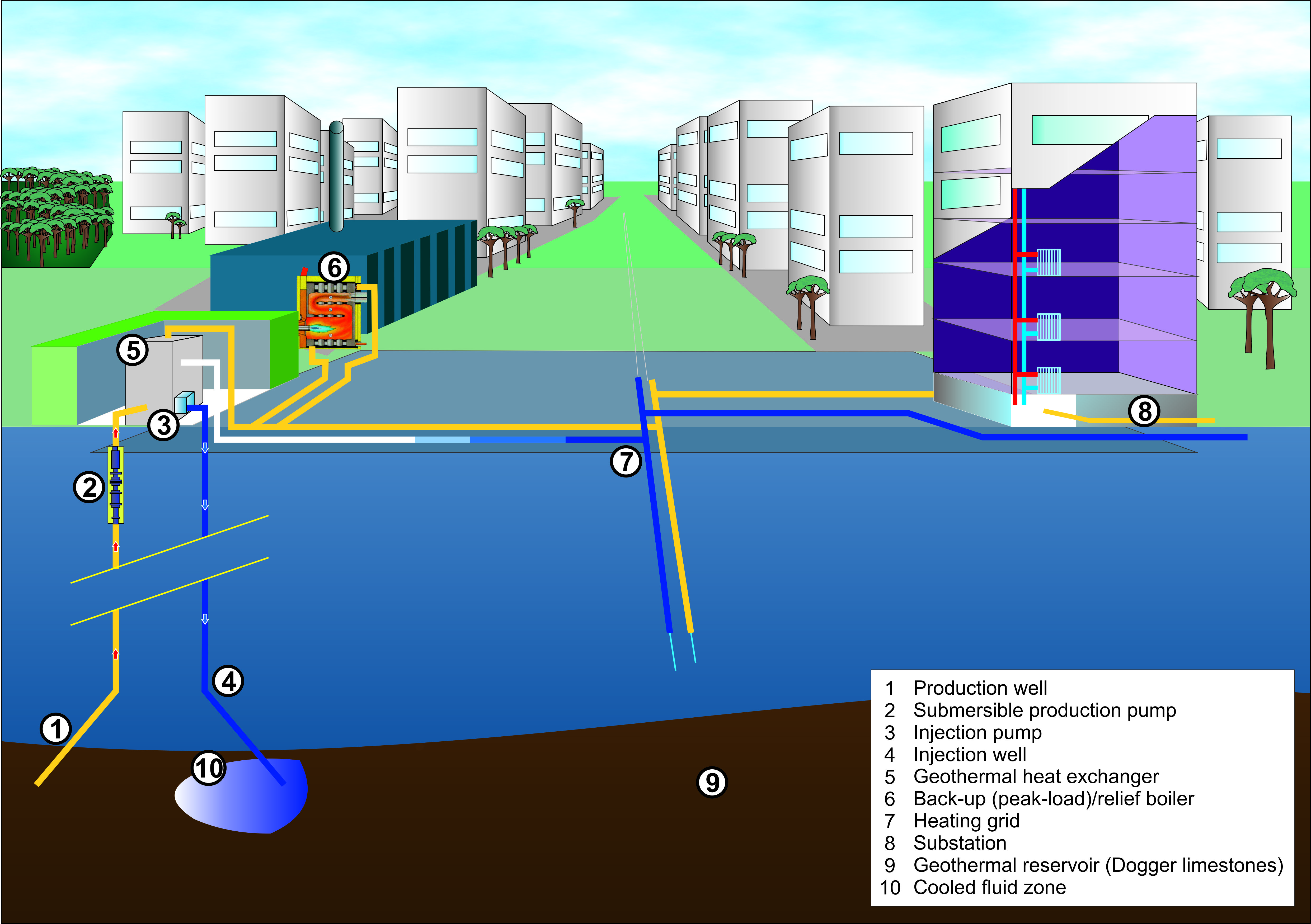
Cite this article

American Association of Petroleum Geologists, Energy Minerals Division. Unconventional Energy Resources: 2017 Review. Nat Resour Res 28, 1661–1751 (2019). https://doi.org/10.1007/s11053-018-9432-1

Download citation

Received: 12 July 2018
Accepted: 07 November 2018
Published: 13 December 2018
Issue Date: October 2019
DOI: https://doi.org/10.1007/s11053-018-9432-1

Keywords

Use our pre-submission checklist

Avoid common mistakes on your manuscript.

Unconventional Energy Resources: 2017 Review

Abstract

Similar content being viewed by others

Unconventional Energy Resources: 2015 Review

New Perspectives for Fossil Fuels: Hydrocarbons in “Unconventional” Settings

Relying on Unconventional Gas Development Projects for the Energy Transition: A Review of Recent Energy History and the Contested Role of Unconventional Gas in France

Introduction

Coal

World Overview and Future Technology Issues

Leading Coal-Producing Countries in 2016

Future Worldwide Coal Production and Consumption

China

India

USA

Future Trends, Production, and Exports

Coal Data Sources

Australia

Indonesia

Russia

South Africa

Germany

Poland

Kazakhstan

Coalbed Methane

Introduction

Summaries of CBM Production for Selected Countries

Tight Gas and Liquids Reservoirs

Introduction

Shale Gas and Liquids

North American Shale Plays

USA

Canada

European Shales

Global Tight Gas Activity

USA

International Tight Gas

Acknowledgments

Bitumen and Heavy Oil

Summary

Acknowledgments

Uranium, Thorium, and Rare Earth Elements Availability and Development: Time for Recovery

Introduction

Uranium Availability

US Sources of Uranium

Industry Response to Uranium Price Fluctuations

The Impact of Japan

Uranium Production in the USA

Fourth Quarter of 2017 Production

Total 2017 Production

Small Nuclear Reactors

Nuclear Waste Storage

Nuclear Power in the Middle Eastern Countries

Other Associated Subjects

Thorium Activities

Rare Earth Activities

Ambient Radiation in the Atmosphere

Radiation Risks and Perspectives

Sources of Radiation

Recent Flux in Magnetic Fields

Uranium (Nuclear and Rare Earth) Committee Reports

Geothermal Energy

Introduction

Geothermal Electrical Power Production

Direct Use

Heat Pumps

Concluding Remarks

Energy Economics and Technology

The Apex of Economic Complexity

Give Up?

The TECH Revolution in Oil and Gas: Taking for Granted What is in Front of our Face

Historical Perspective

Historical Perspective: 1970s Fuel Insecurity

Historical Perspective: 1980s—Gas Bubble, Coal, Environment, Boom

Historical Perspective: The End of the Bubble

Historical Perspective: Hello, Shales! July 2008 Triggers New Thinking

Issues of the Day

US Tight Oil/Shale Oil Still Major Influence on Global Oil Prices

Bankruptcy Surge in 2016 and Other Negatives

So Many Questions

Notes