Cohesive zone models and impact damage predictions for composite structures

Abstract

This article surveys existing cohesive zone models (CZM) and their use in numerical simulations for analysis impacts on composite structures and predicting the damage induced. These models are used for matrix cracks and delamination. The first part of article gives the required background on failure criteria for predicting the onset of delaminations, on fracture mechanics and the various types of CZM. The second part discusses applications of CZM to several types of impact problems with composite structures. Applications for these models to other problems are briefly mentioned at the end. CZM are now part of state of the art numerical simulations with progressive damage analysis.

1 Introduction

Predicting impact induced damage in composite structures requires the ability to predict the onset of the various damage modes and the growth of that damage during the impact. Cohesive zone models (CZM) used to predict the growth of various types of cracks are reviewed in this article with a special focus on impact problems. These models are generally used in a numerical progressive damage analysis that accounts for damage development and the degradation of the properties of the plies and the interfaces. This article provides an overview of cohesive zone models including their connection to fracture mechanics and their use in prediction impact damage in composite structures. Such damage prediction requires failure criteria to determine when damage initiates and the study of the subsequent damage propagation. The article presents a brief overview of the failure criteria used to predict damage initiation including delamination. With CZMs, the propagation of delaminations is based on a fracture criterion so some basic concepts from fracture mechanics are added to make the presentation self-contained and easier to follow. CZMs are included in several commercial finite element codes and are widely used for various applications. In the analysis of impact damage on composite structures, this article will show that CMZs have resulted in accurate predictions that were not previously possible and greater insights.

Several types of damage can be induced: (1) interply debonding or delamination; (2) intraply damage in the form of shear cracks, bending cracks, and fiber failure. These two types of damage interact to create complex patterns. At a microscopic level, fiber-matrix debonding and microscopic matrix cracks develop and eventually coalesce and form failure surfaces at the ply level. Foreign object impacts can cause delaminations and matrix cracks that can severely reduce the load carrying capacity of the structure [1]. Delaminations also occur when discontinuities induce interlaminar stress concentrations. Examples include: free edges, holes, matrix cracks, ply drop offs, bonded joints, and bolted joints. Extensive research has been conducted on delaminations since this type of failure is induced rather easily and can have a dramatic effect on the residual properties. Several reviews of the literature on delaminations in composite structures are available [2–6]. Failure criteria for predicting the onset of delamination are discussed in Sect. 2.

Once an interfacial crack is created, its propagation under load should be determined using a fracture mechanics approach. Basic fracture mechanics concepts are recalled and their application to the propagation of delaminations is discussed in Sect. 3 that includes a discussion of widely used numerical technique called the Virtual Crack Closure Technique (VCCT). In recent years, the propagation of delaminations and matrix cracks has been analyzed using CZM that are presented in Sect. 4. Applications of the CZM to study damage in composite structures is discussed in Sect. 5 with emphasis on foreign object impacts on composite and sandwich structures and energy absorbing structures made out of composite materials.

2 Failure criteria for predicting the onset of delamination

Debonding between adjacent layers depends on the stresses acting on that interface: the normal componentand the two shear stresses and $\sigma_{23}$. References [7–9] predicted delamination using a maximum stress criterion for the normal stress and a quadratic criterion for the two shear components

$$ \sigma_{33} /Z_{T} \ge 1\;\quad {\text{or}}\quad \;\left( {\frac{{\sigma_{23} }}{{S_{3} }}} \right)^{2} + \left( {\frac{{\sigma_{13}^{{}} }}{{S_{3}^{{}} }}} \right)^{2} \ge 1 $$

(2.1)

$\sigma_{33}$ where S₃ is the shear strength and Z_T $\sigma_{13}$ the tensile strength in the thickness direction. It is assumed that no failure occurs when $\sigma_{33} < 0$. The criterion proposed by Christensen and DeTeresa [10]

$$ \left( {\frac{{\sigma_{13} }}{{S_{13} }}} \right)^{2} + \left( {\frac{{\sigma_{23} }}{{S_{23} }}} \right)^{2} \ge 1 $$

(2.2)

allows for different strengths for $\sigma_{13}$ and $\sigma_{23}$ but does not account for interactions between the normal and shear stresses acting at the interface.

Several criteria accounting for the interaction between the three stress components acting at the interface have been introduced. References [11–19] postulated that the onset of delamination is governed by

$$ \left( {\frac{{\sigma_{33} }}{{Z_{T} }}} \right)^{2} + \left( {\frac{{\sigma_{13} }}{{S_{13} }}} \right)^{2} + \left( {\frac{{\sigma_{23} }}{{S_{23} }}} \right)^{2} \ge 1\quad {\text{when}}\quad \sigma_{33} > 0 $$

(2.3)

where S₁₃ and S₂₃ are the shear strength in the through-thickness and fiber plane. Again, References [12, 16, 17, 20] assumed that S₁₂ = S₂₃. Cesari et al. [11] used the same criterion when $\sigma_{33} < \,\,0$ but with Z_c (compressive strength in the through-thickness direction) instead of Z_T in that case. The ellipsoid defined by Eq. 2.3 accounts for the interaction between the three stress components acting at the interface.

References [8, 21–26] use the delamination criterion proposed by Choi and Chang [27]. In the latter, originality lies in the fact that the stresses are averaged over the thickness of the layer above the interface (layer n + 1) and the strengths can be those of either the layer above or the layer below (n).

The quadratic delamination criterion of Brewer and Lagace [28] is similar to Eq. (2.3) and can be written as

$$ \left( {\frac{{\sigma_{33} }}{Z}} \right)^{2} + \left( {\frac{{\sigma_{13} }}{{S_{13} }}} \right)^{2} + \left( {\frac{{\sigma_{23} }}{{S_{23} }}} \right)^{2} \ge 1 $$

(2.4)

where Z = Z_t when $\sigma_{33} > \,\,0$ and Z = Z_c when $\sigma_{33} < \,\,0$. Thus, the value of Z makes the difference between tensile normal stress (that are opening) and compressive normal stress (that are closing). Naik et al. [29–31] used Eq. 2.4 and averaged the values of the stresses through the thickness of the ply. Li et al. [32] used the Brewer-Lagace criterion as defined when $\sigma_{33} > \,\,0$ and omitted the effect of the transverse normal stress when $\sigma_{33} < \,\,0$. In that case, we recover the criterion proposed by Yeh and Kim [33] which predicts that tensile delaminations occurs when $\sigma_{33} > 0$ and

$$ \left( {\frac{{\sigma_{33} }}{{Z_{T} }}} \right)^{2} + \left( {\frac{{\sigma_{13} }}{{S_{13} }}} \right)^{2} + \left( {\frac{{\sigma_{23} }}{{S_{23} }}} \right)^{2} \ge 1 $$

(2.5)

and shear delaminations occurs when σ₃₃ < 0 and

$$ \left( {\frac{{\sigma_{13} }}{{S_{13} }}} \right)^{2} + \left( {\frac{{\sigma_{23} }}{{S_{23} }}} \right)^{2} \ge 1 $$

(2.6)

Equation 2.6 is identical to Eq. 2.2, the criterion proposed by Christensen and DeTeresa [10]. Huang and Lee [25], Liu and Wang [34] used Yeh’s criterion (Eqs. 2.5, 2.6).

Zhao and Cho [18] used only the tensile part of the criterion (Eq. 2.5). Chen [35] included the effect of the in-plane transverse stress σ₂₂ and predict a damage propagation between the layer (n) and (n + 1) by the relation

$$ \left( {\frac{{{}^{n}\sigma_{33} }}{{Z_{C} }}} \right)^{2} \,+\, D_{1} \left( {\frac{{{}^{n}\sigma_{23}^{2} + {}^{n + 1}\sigma_{13}^{2} }}{{S^{2} }}} \right) + D_{2} \left( {\frac{{{}^{n + 1}\sigma_{22} }}{Y}} \right)^{2} = e_{D} $$

(2.7)

where Y represents the in-plane transverse tensile (σ₂₂ ≥ 0) or compressive (σ₂₂ < 0) strength of laminates. D₁, D₂ are experimental constants and they are only related to the material properties of laminates. Damage occurs when $e_{D} \ge 1$.

Hou et al. [13, 14] assumed that delamination occurs when

$$\left( {\frac{{\sigma_{33} }}{{Z_{T} }}} \right)^{2} + \frac{{\sigma_{23}^{2} + \sigma_{13}^{2} }}{{S_{13}^{2} \left( {d_{ms} d_{fs} + \delta } \right)}} \ge 1\quad {\text{when}}\quad \sigma_{33} \ge 0 $$

(2.8)

or

$$ \frac{{\sigma_{23}^{2} + \sigma_{13}^{2} - 8\sigma_{33}^{2} }}{{S_{13}^{2} \left( {d_{ms} d_{fs} + \delta } \right)}} \ge 1\quad {\text{when}}\quad - \sqrt {\left( {\sigma_{23}^{2} + \sigma_{13}^{2} } \right)/8} \le \sigma_{33} < 0 $$

(2.9)

They also assumed that no delamination occurs when

$$ \sigma_{33} < - \sqrt {\left( {\sigma_{23}^{2} + \sigma_{13}^{2} } \right)/8} $$

(2.10)

In Eqs. (2.8, 2.9), d_ms is a damage coefficient of matrix cracking and d_fs is a damage coefficient of fibre failure and δ is the ratio between interlaminar stresses before and after matrix or fiber failure.

Zou et al. [13, 14] proposed a single criterion that accounts for different strength for tension and compression in the transverse direction and for the effect of the two transverse shear stresses

$$ \frac{{\sigma_{33}^{2} }}{{Z_{t} Z_{c} }} + \frac{{\sigma_{13}^{2} + \sigma_{23}^{2} }}{{S^{2} }} + \left( {\frac{1}{{Z_{t} }} - \frac{1}{{Z_{c} }}} \right)\sigma_{33} \ge 1 $$

(2.11)

Fenske and Vizzini [36] extended the Brewer-Lagace criterion by including the effects of inplane stresses.

These various criteria attempt to predict the onset of delamination at the interface between two adjacent plies in terms of the stresses acting at that interface. It is important to remember that the behavior is very different depending on the sign of the transverse normal stress.

3 Fracture mechanics approach

Once interface failure is predicted, the stress distribution in the surrounding material becomes singular and the presence of the crack should be accounted for in the analysis. This section presents a brief historical overview of the development of fracture mechanics followed by a discussion of its application to the propagation of delaminations at bimaterial interfaces, and an introduction to the Virtual Crack Closure Technique (VCCT) used for numerical simulations.

3.1 Historical background

Initially, the first studies concerning fracture mechanics, which are recalled in this part, were focused on crack propagation in isotropic metallic materials. The later developpements of fracture mechanics theories for orthotropic materials are based on these theories.

Leonardo da Vinci (1452–1519) conducted tests to determine the strength of iron wires and found an inverse relationship between the strength and the length of the wire [37]. This early evidence of a size effect was confirmed by several other experiments on iron bars and wires and glass fibers. A possible explanation for this size effect is the presence of flaws in the material that would significantly reduce the strength.

In 1898, Kirsch (in [38]) studied the stress concentrations created by a circular hole in a plate subjected to uniaxial tension and, in 1913, Inglis [39] extended that work to determine the stress field around a plate containing an elliptical rather than circular hole (Fig. 1). It was shown that, at the end of the major axis of the ellipse, the normal stress in the tangential direction is given by

$$ \sigma_{y} \, = \sigma \,\,\left( {1 + 2\sqrt {a/\rho } } \right) $$

(3.1)

where $\sigma \,$ is the remote stress, a is the length of the major semi-axis which is perpendicular to the loading direction, and $\rho$ is the radius of curvature at the end of the major axis of the ellipse. As becomes much smaller than a, $\sigma_{y}$ becomes infinite. This result would imply that for a body with a sharp crack the strength would be near zero. For a circular hole, $a = \rho$ and Eq. (3.1) gives the well-known result $\sigma_{y} \, = 3\sigma \,$ in that case.

Fig. 1

Elliptic flaw in an infinite plate subjected to a uniaxial stress

The work of Griffith [40] was motivated by the fact that the bulk strength of glass (172 MPa) was much smaller than the strength of a thin glass tube (2372 MPa) or that of glass fibers (1500–6200 MPa) [37]. Griffith introduced an artificial flaw in specimens (Fig. 2) and experimental results indicated that, at fracture, the product $\sigma \,\sqrt a$ remained nearly constant.

Fig. 2

An edge crack flaw in a material

Westergaard [41] showed that the stress near a crack tip for infinite plate and through thickness cracks is approximately equal to

$$ \begin{aligned} \sigma_{x} &= \frac{{K_{I} }}{{\sqrt {2\pi r} }} \cdot \cos \frac{\theta }{2}\left( {1 - \sin \frac{\theta }{2}\sin \frac{3\theta }{2}} \right) \hfill \\ \sigma_{y}& = \frac{{K_{I} }}{{\sqrt {2\pi r} }} \cdot \cos \frac{\theta }{2}\left( {1 + \sin \frac{\theta }{2}\sin \frac{3\theta }{2}} \right) \hfill \\ \sigma_{xy} &= \frac{{K_{I} }}{{\sqrt {2\pi r} }} \cdot \cos \frac{\theta }{2}\sin \frac{\theta }{2}\cos \frac{3\theta }{2} \hfill \\ \end{aligned} $$

(3.2)

where $K_{I} = \sigma \sqrt {\pi a}$ is the stress intensity factor for mode I fracture, r is the distance from the crack tip and $\theta$ is the orientation angle (Fig. 3). Near the crack tip, the stress is maximum for $\theta = 0$ and

$$ \upsigma_{{\rm y}} |_{\theta = 0} = \upsigma {\sqrt{\frac{{\rm a}}{2{\rm r}}}} = \frac{\upsigma {\sqrt {\pi {\rm a}}}}{{\sqrt {2\pi {\rm r}}}} = \frac{{\rm K}_{{\rm I}}}{{\sqrt {2\pi {\rm r}}}} $$

(3.3)

The stress is singular at the crack tip and the singularity is of order r^−1/2.

Fig. 3

Cylindrical coordinates at crack tip

Irwin [42] studied this problem for an infinite plate and plane stress conditions. He showed that for isotropic ductile materials a plastic zone is created near the crack tip and that the total energy release rate G is the sum of the surface energy release rate $2\gamma$ and a plastic energy release rate G_p. For brittle materials such as glass the surface energy release rate dominates and $G \approx 2\gamma = 2\,{\text{J}}/{\text{m}}^{2}$. For ductile materials such as steel G_p dominates and $G \approx 1000 {\text{J}}/{\text{m}}^{2}$.

$$ \sigma_{f} \sqrt {\pi a_{c} } = \sqrt {GE} $$

(3.4)

G is the strain energy release rate and E is the Young modulus.

So far, we discussed the effect of a Mode I crack—Opening mode with a tensile stress normal to the plane of the crack. Figure 4 shows two other fracture modes:

Fig. 4

The three fracture modes: a Mode I; b Mode II; c Mode III

• Mode II crack—Sliding mode (a shear stress acting parallel to the plane of the crack and perpendicular to the crack front)

• Mode III crack—Tearing mode (a shear stress acting parallel to the plane of the crack and parallel to the crack front)

Three stress intensity factors can be defined as

$$ \left\{ {\begin{array}{*{20}c} {K_{I} } \\ {K_{II} } \\ {K_{III} } \\ \end{array} } \right\} = \mathop {\lim }\limits_{r \to 0} \sqrt {\pi r} \left\{ {\begin{array}{*{20}c} {\sigma_{22} } \\ {\sigma_{12} } \\ {\sigma_{23} } \\ \end{array} } \right\} $$

(3.5)

Failure criteria described in Sect. 2 can be used to predict the onset of delamination. Once initiated, the propagation of a delamination is a dynamic fracture event. A Griffith type criteria can be used to determine whether an existing delamination extends or not based on the value of the total strain energy release rate: the delamination does not extend if $G \le G_{c}$ and it extends if $G > G_{c}$. This approach requires a detailed stress analysis near the crack tip and the ability to calculate the change in strain energy as the delamination increases by a small amount. However, it does not require knowledge of the individual strain energy release rates G_I, G_II, G_IlI.

In general it is assumed that a mixed-mode failure criterion can be developed in the following form

$$ f\left( {\frac{{G_{I} }}{{G_{IC} }},\,\,\frac{{G_{II} }}{{G_{IIC} }},\,\,\frac{{G_{III} }}{{G_{IIIC} }}} \right) \ge 1 $$

(3.6)

In developing such a criterion, the two challenges are: determining the form of the function f and conducting tests to identify the critical energy release rates and other parameters that may be present in specific failure criteria. The developments of fracture mechanics for composite materials are based on the principles defined for isotropic materials. Examples of mixed-mode failure criteria are the power law criterion

$$ \left( {\frac{{G_{I} }}{{G_{IC} }}} \right)^{\alpha } + \left( {\frac{{G_{II} }}{{G_{IIC} }}} \right)^{\alpha } = 1 $$

(3.7)

first introduced by Wu and Reuter [43] and the Benzeggagh and Kenane criterion [44]

$$ G_{TC} = G_{IC} + \left( {G_{IIC} - G_{IC} } \right)\left( {\frac{{G_{II} }}{{G_{T} }}} \right)^{\alpha } $$

(3.8)

where $G_{T} = G_{I} + G_{II}$ is the total energy release rate, $G_{TC}$ is the total critical energy and $\alpha$ is a parameter. Mixed-mode fracture criteria are needed in the formulation of cohesive elements and the two mentioned here (Eqs. 3.7, 3.8) are the most commonly used.

3.2 Fracture mechanics approach to delamination propagation

Fracture mechanics can be used to study the propagation of impact induced delaminations at ply interfaces. The objective is to predict the extent of delaminations at each interface. Individual plies may have cracks because of matrix failure due to tensile bending stresses, transverse shear stresses, or residual thermal stresses [45]. The second objective is to determine whether these matrix cracks will lead to interface debonding.

Interfacial cracks between two isotropic materials with different elastic properties have been studied extensively, For cracks at the interface of two isotropic bodies with different elastic properties, single mode loading produces both opening and shearing modes (Williams [46]). For a bimaterial interfacial crack, the near-tip normal and shear stresses are given by

$$ \sigma_{yy} + i\sigma_{xy} = \frac{{\left( {K_{I} + iK_{II} } \right)r^{i\varepsilon } }}{{\sqrt {2\pi r} }} $$

(3.9)

where $i = \sqrt { - 1} , \, K_{I} \quad {\text{and}}\quad K_{II}$ are components of the complex stress intensity factor K = K_I + iK_II and $\varepsilon$ is the oscillation index

$$ \varepsilon = \frac{1}{2\pi }\ln \left[ {\frac{1 - \beta }{1 + \beta }} \right] $$

(3.10)

where $\beta$ is one of two Dundurs constants. For plane strain, the Dundurs constants are

$$ \alpha = \frac{{\bar{E}_{1} - \bar{E}_{2} }}{{\bar{E}_{1} + \bar{E}_{2} }}\quad \beta = \frac{{G_{1} \left( {1 - 2\nu_{2} } \right) - G_{2} \left( {1 - 2\nu_{1} } \right)}}{{2\left[ {G_{1} \left( {1 - 2\nu_{2} } \right) + G_{2} \left( {1 - 2\nu_{1} } \right)} \right]}} $$

(3.11)

where $\bar{E} = E/\left( {1 - \nu^{2} } \right)$. E is the elastic modulus, G is the shear modulus, $\nu$ is Poisson’s ratio and the subscripts 1 and 2 refer to the materials above and below the interface. Stresses oscillate as the distance from the crack tip increase, as indicated by the $r^{i\varepsilon }$ term in Eq. 3.9, but this oscillation is limited to a very small region near the crack tip [47]. The individual rates G_I and G_II oscillate very close to the crack tip but Mulville and Mast [48] showed that the total strain energy release rate remains almost constant as the crack propagates. When the materials above and below the interface are identical, $\varepsilon = 0,\;\alpha = 0,\;\beta = 0$. Then, stresses do not oscillate as expected for a crack in a homogeneous material.

A crack impinging on an interface joining two dissimilar materials may arrest or may advance by either penetrating the interface or deflecting into the interface (Fig. 5). He and Hutchinson [49] showed that, in order for a crack impinging the interface at any angle to be deflected, the toughness of the interface must be less than one quarter of the toughness of the material on the other side of the interface when $- 0.5 < \alpha < 0.25$. It was shown that residual thermal stresses have a significant effect on this problem [50].

Fig. 5

Several scenarios for a crack impinging on a bi-material interface

He and Hutchinson [51] studied the kinking of a crack out of an interface (Fig. 6). Assuming that the condition for propagation in the interface is G_o = G_oc and that for propagation in material 2, G_II = G_IIc. If G_IIc is sufficiently large compared to G_oc the crack does not kink into material 2. If these two critical energy release rates are comparable there is a loading range such that the crack stays in the interface and above that the crack will kink into material 2. Ryoji [52] gave a stress-based criterion for predicting the kink angle. Rudas [53] gave a simple formula for predicting the kink angle based on the mode mixity ratio K_I/K_II. Carlsson and Prasad [54–56] used the results obtained in [51] to study interfacial cracks in sandwich structures and the kinking of these cracks into the core.

Fig. 6

Geometry for crack kinking of a bi-material interface [51]

Experiments using a modified DCB (Double Cantilever Beam) specimen to produce high speed Mode I crack propagation showed that the Mode I dynamic fracture toughness of unidirectional AS4/3501-6 is equal to the static fracture toughness for crack speeds up to 200 m/s [57]. Dynamic delamination experiments on modified ENF specimens of unidirectional AS4/3501-6 graphite/epoxy composite under three point bending showed that the dynamic fracture toughness is not affected significantly by crack speed up to 1100 m/s [58, 59]. Dynamic initiation fracture toughness of S2/8552 and IM7/977-3 composites were obtained using a wedge insertion fracture (WIF) test method indicated that both the dynamic initiation fracture toughness and the fracture toughness during dynamic delamination cracking at speeds up to 1000 m/s remain approximately equal the static fracture toughness [60]. Studies of the effects of loading rates on fracture toughness for composites include Refs [61, 62] for mode I, [48, 63–66] for mode II, and [67] for mode III.

Analytical studies of dynamic interfacial crack propagation were presented by Gol’dshtein [68], Brock and Achenbach [69], Atkinson [70], Willis [71], Deng [72]. Willis [71] presented a two-dimensional analysis of the stress field around a crack on the plane interface between two bonded dissimilar anisotropic elastic half-spaces. Yang et al. [73] examined the singular fields around a crack running dynamically along the interface between two anisotropic substrates.

Experimental studies of dynamic interface crack propagation started with the work of Tippur and Rosakis [74] in 1991. In a homogeneous solid, the crack tip velocity cannot exceed the Rayleigh wave speed of the material [75]. A series of experiments [76–83] showed that, at the interface of bimaterial plates, crack tip velocities between steel and PMMA (polymethylmethacrylate) can reach the intersonic regime. That is, the range between the shear wave velocity and the longitudinal wave velocity of PMMA. Large scale contact behind the crack tip is observed when $c_{s} < v < \sqrt 2 c_{s}$. An analysis of these experiments confirms those experimental findings [84].

A study of dynamic crack growth along the interface of a fiber-reinforced polymer composite–homalite bimaterial subjected to impact shear loading [85] led to the first conclusive experimental evidence of interfacial crack speeds faster than any characteristic elastic wave speed of the more compliant material and the first experimental observation of a mother–daughter crack mechanism allowing a subsonic crack to evolve into an intersonic crack.

Lambros and Rosakis [86] applied the same experimental techniques to laminated composite plates. In [87] laminated composite plates where subjected to transverse impacts and delamination speeds measured ranged from 500–1800 m/s. Accurate optical measurements of the transverse displacements were used to estimate the size of delaminations and the speed at which they grew.

Elder et al. [88] provide a quick overview of currently available methods for predicting delaminations induced by low velocity impacts. Davies et al. [89–94] presented a very simple approach to predict the delamination threshold load (DTL) using a simply supported circular plate and a clamped circular plate with an existing delamination of radius a located on the midplane (Fig. 7). For plates without a delamination, bending stresses are zero and transverse shear stresses reach a maximum on the midplane. One can then expect that delaminations might occur on the midplane under mode II fracture.

Fig. 7

Simplified model for predicting the delamination damage threshold load [375]

The deflection of the central portion an undamaged clamped plate of thickness 2 h under the force P is

$$ \delta_{u} = \frac{{3Pa^{2} \left( {1 - \nu^{2} } \right)}}{{4\pi E\left( {2h} \right)^{3} }} $$

(3.12)

The central portion of the damaged plate can be considered as two plates each having a thickness h and subjected to a force P/2. The deflection of the central portion of the damage plate is then

$$ \delta_{d} = 3\frac{P}{2}\frac{{a^{2} \left( {1 - \nu^{2} } \right)}}{{4\pi Eh^{3} }} $$

(3.13)

The energy available to drive the crack is

$$ U = \frac{1}{2}P\left( {\delta_{d} - \delta_{u} } \right) = \frac{{9P^{2} a^{2} \left( {1 - \nu^{2} } \right)}}{{64\pi Eh^{3} }} $$

(3.14)

As the crack advances from a to $a + \delta a,\;G.2\pi a\delta a = \frac{\partial U}{\partial a}\delta a$. The DTL is then given by

$$ P_{c}^{2} = \frac{{64\pi^{2} Eh^{3} }}{{9\left( {1 - \nu^{2} } \right)}}G_{IIc} $$

(3.15)

which indicates that this load is independent of the initial radius of the delamination, that it depends of the Mode II critical energy release rate, and that it varies with h^3/2. Schoeppner and Abrate [95] showed that the DTLs predicted by this equation are in good agreement with experimental results for a large number of tests. Equation 3.15 is also used by Olsson [96–99] and others (e.g. [100]) to predict the DTL.

3.3 Virtual crack closure technique

The finite element method is used extensively in linear elastic fracture mechanics and a first review of the literature is presented by Banks-Sills [101, 102]. The virtual crack closure technique (VCCT) proposed by Rybicki and Kanninen [103] is widely used and several reviews have been presented by Krueger [104]. The principle of the two-step VCCT [104] can be described as follows:

• 1. A finite element model is used to model a solid with pairs of coincident nodes coupled together ahead of the crack (Fig. 8a).

  Fig. 8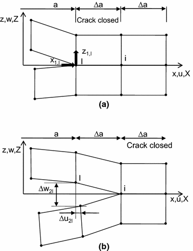

  

  Two step VCCT. a First step—crack closed. b Second step—crack extended

• 2. When the load reaches a critical value, the coupled nodes at the crack tip are released and the crack extends one element length $\Delta a$(Fig. 8b).

• 3. The energy released during the crack extension is assumed to be equal to the energy required to close the crack extension back.

$$ \Delta E = \frac{1}{2}\left[ {X_{1L} \cdot \Delta u_{2L} + Z_{1L} \cdot \Delta w_{2L} } \right] $$

(3.16)

where $\Delta u_{2L}$ and $\Delta w_{2L}$ are the differences in shear and opening displacements at node L in the second finite element model and X_1L and Z_1L are the forces applied at node L in the first model to close the crack extension.

The modified VCCT or one-step VCCT is illustrated in Fig. 9. Considering the extension of the crack from node i to node k, it is assumed that the displacements at node i after the extension will be the same as those at node L in the current configuration. The forces shown at node i are those needed to prevent the extension from i to k. The energy released is

$$ \Delta E = \frac{1}{2}\left[ {X_{i} .\Delta u_{L} + Z_{i} .\Delta w_{L} } \right] $$

(3.17)

Using four-noded elements as in Fig. 9, the mode I and mode II energy release rates are given by

$$ G_{I} = \frac{1}{2\Delta a}Z_{i} .\Delta w_{L},\quad G_{II} = \frac{1}{2\Delta a}X_{i} .\Delta u_{L} $$

(3.18)

Bonhomme et al. in [105], determine the energy release rate under mode I in a AS4/8552 carbon/epoxy laminates by the one step and the two step VCCT method. Results were compared with empirical data obtained from double cantilever beam (DCB) tests. Both one and and Two-step VCCT methods converge as element length decreases.

Fig. 9

Modified VCCT or one-step VCCT

Extensions of this basic approach to 2D problems modeled usind 8-noded elements, to 3D problems using solid elements and problems modeled using plate or shell elements are discussed in Krueger [104]. The additional dimension allowed to calculate the distribution of the energy release rates along the delamination front and makes it possible to obtain G_III.

The use of elements with quadratic shape functions gives a kinematically incompatible interpenetration which caused initial problems. Element-wise opening (where edge and midside nodes are released) corrects this and yields reliable results.

Special attention should be given to the calculation of the strain energy release rate components when the element lengths (Δa) for the element in front of the crack tip and behind are not identical. The following relationships, which only depend on the length of the elements in front and behind the crack tip, account for this effect.

$$ G_{I} = \frac{1}{{2\Delta a_{1} }}Z_{i} \cdot \Delta w_{L} \cdot \left( {\frac{{\Delta a_{2} }}{{\Delta a_{1} }}} \right)\quad G_{II} = \frac{1}{{2\Delta a_{1} }}X_{i} \cdot \Delta u_{L} \cdot \left( {\frac{{\Delta a_{2} }}{{\Delta a_{1} }}} \right) $$

(3.19)

where Δa₁ and Δa₂ are the element length in front and behind the crack tip. A similar correction can be used when the elements along the delamination front have different widths.

The modified VCCT is used in [101, 102] to characterize respectively the energy release rate in mode I, mode II, mode III, mixed mode I + II of glass/epoxy laminates and the energy release rate in mode I of carbon fiber reinforced composites. Improvements for tracking delamination fronts made by Pietropaoli and Riccio [105–108] consist in adapting the load step size to the size of the mesh by an iterative calculation until the convergence is reached, which corresponds to the superposition of the crack front with mesh nodes. To allow more complex shapes of the delamination front to be taken into account, this improvements is associated with the use of weight factors expressed in terms of fraction of debonded area in order to take into account the node position in the delaminated lobe.

The VCCT method is used by Yoshimura [109] to calculate the energy release rate of the delamination crack in a stitched carbon fiber reinforced composite laminate. In order to consider the bridging effect, a linear spring element is used to connect the neighboring layer. Simulation results revealed that the improvement in impact damage resistance due to stitching became greater as the delamination area grew larger.

4 Cohesive element approach

The virtual crack closure technique used to estimate the energy release rates has several drawbacks: (1) it requires a very fine mesh near the interfacial crack tip; (2) an existing crack with given shape and size is needed; (3) it requires complex moving mesh techniques to advance the crack front. A different approach has been developed recently and is used extensively for studying delaminations in composite materials and failure of bonded joints. This approach is based on the cohesive zone concept proposed by Barenblatt [110, 111] and Dugdale [112]. It is assumed that ahead of the crack tip, there is a very thin layer separating two solids in which the damage mechanisms leading to fracture are localized. The behavior of this fracture process zone is characterized by a traction–separation law called the cohesive law. Shet and Chandra [113] listed eleven popular CZM with different cohesive laws. Cohesive laws are classified into two categories: (a) intrinsic cohesive laws that have an initial elastic slope; and (b) extrinsic cohesive laws that are initially rigid [114].

For finite element analyses, several types of elements based on this CZM were developed to model the behavior of the interface. These elements called “cohesive elements” or “decohesion elements” can be: (1) point decohesion elements or discrete cohesive elements [115–118] which are essentially three dimensional nonlinear springs; (2) continuous decohesion elements connecting line elements, 2D or 3D solid elements, or plate or shell elements. This strategy allows the modelling of complex shapes by the use of refined meshes.

Considering the interface between two elastic layers, Fig. 10 shows the lower layer, the interface, the delamination front, and the local coordinate system to be used in the following. The x₁-x₂ plane is the plane of the interface, x₃ is normal to the interface, and the delamination extends in the x₁ direction. In that coordinate system, stresses acting on the interface have two shear components $\tau_{1}$ and $\tau_{2}$, and one normal component $\tau_{3}$. At a given point on the interface, two nodes are initially in contact: one is on the lower layer and the other is on the upper layer. The displacements of the upper and lower layers are denoted by $u_{i}^{U}$ and $u_{i}^{L}$ where i = 1, 2, 3. The relative displacements defined by $\delta_{i} = u_{i}^{U} - u_{i}^{L}$ consist of two sliding displacements (δ₁ and δ₂) and one opening displacement $\delta_{3}$.

Fig. 10

Coordinate system at a delaminating interface

The behavior of the interface is defined by a cohesive law that relates the relationship between the interfacial stresses and the relative displacements. Many cohesive laws have been formulated [119]. Indeed, CZMs have been used to simulate the fracture process in a number of material systems and under various loading conditions. Here, the cohesive laws most used in the frameworks of impacts on composite structures are presented. The use of cohesive elements for the modelling of interlaminar and intralaminar cracks in composite laminates under impact is treated in part 5.

4.1 Bilinear cohesive law

The most commonly used cohesive law used in the development of cohesive elements is the bilinear law illustrated in Fig. 11 for pure mode I fracture. The normal stress $\tau_{3}$ increases linearly with the relative displacement $\delta_{3}$ until the onset of the decohesion process when these two quantities reach the critical values N and softening is observed as the relative displacement increases beyond $\delta_{3}^{o}$ as shown in the figure. Complete failure of the interface occurs when $\tau_{3} = 0$ and the displacement reaches its final value. The area under the curve is the energy dissipated in the process and must be equal to the critical energy release rate G_Ic in this case.

Fig. 11

Bilinear cohesive law

The behavior of the cohesive zone is assumed to be similar for Mode II and pure Mode III loading. Therefore, the behavior for the initial phase can be written as

$$ \tau_{i} = k_{i} \delta_{i} $$

(4.1)

where k_i is the initial stiffness of the interface. If the limits for the tractions in the tangential directions and the normal direction are T, S, and N, then

$$ \delta_{1}^{o} = T/k_{1} ,\quad\delta_{2}^{o} = S/k_{2},\quad\delta_{3}^{o} = N/k_{3} $$

(4.2)

The area under the curves must be equal to the corresponding critical strain energy release rate. That is,

$$ G_{Ic} = \int_{o}^{{\delta_{3}^{f} }} {\tau_{3} d\delta_{3} } ,\quad G_{IIc} = \int_{o}^{{\delta_{1}^{f} }} {\tau_{1} d\delta_{1} } ,\quad G_{IIIc} = \int_{o}^{{\delta_{2}^{f} }} {\tau_{2} d\delta_{2} } $$

(4.3)

Therefore, for this bilinear cohesive law, the relative displacements at failure are

$$ \delta_{1}^{f} = 2G_{IIc} /T,\quad\delta_{2}^{f} = 2G_{IIIc} /S,\quad\delta_{3}^{f} = 2G_{Ic} /N $$

(4.4)

In the case of mixed mode loading, the relative displacements are $\delta_{1m} ,\,\delta_{2m} ,\delta_{3m}$ where the subscript m is added to distinguish quantities for mixed mode loading from the same quantities in the case of pure mode loading. Introducing the normalized relative displacements $\lambda_{i} = \delta_{im} \,/\,\delta_{i}^{f}$, the total effective relative displacement is defined as

$$ \lambda = \sqrt {\lambda_{1}^{2} + \lambda_{2}^{2} + \lambda_{3}^{2} } $$

(4.5)

Under mixed mode loading the decohesion process starts when $\lambda$ reaches a value

$$ \lambda^{o} = \sqrt {\left( {\lambda_{1}^{o} } \right)^{2} + \left( {\lambda_{2}^{o} } \right)^{2} + \left( {\lambda_{3}^{o} } \right)^{2} } = \sqrt {\left( {\frac{{\delta_{1m}^{o} }}{{\delta_{1}^{f} }}} \right)^{2} + \left( {\frac{{\delta_{2m}^{o} }}{{\delta_{2}^{f} }}} \right)^{2} + \left( {\frac{{\delta_{3m}^{o} }}{{\delta_{3}^{f} }}} \right)^{2} } $$

(4.6)

Complete failure occurs when

$$ \lambda^{f} = \sqrt {\left( {\lambda_{1}^{f} } \right)^{2} + \left( {\lambda_{2}^{f} } \right)^{2} + \left( {\lambda_{3}^{f} } \right)^{2} } = \sqrt {\left( {\frac{{\delta_{1m}^{f} }}{{\delta_{1}^{f} }}} \right)^{2} + \left( {\frac{{\delta_{2m}^{f} }}{{\delta_{2}^{f} }}} \right)^{2} + \left( {\frac{{\delta_{3m}^{f} }}{{\delta_{3}^{f} }}} \right)^{2} } $$

(4.7)

A stress based failure criterion is used to determine $\lambda^{o}$ and a mixed mode fracture criterion is used to determine $\lambda^{f}$.

During the unloading phase $\left( {\lambda^{o} \le \lambda \le \lambda^{f} } \right)$ the tractions reduce linearly according to

$$ \tau_{i} = k_{i} \frac{{\lambda^{o} }}{\lambda }\frac{{\lambda^{f} - \lambda }}{{\lambda^{f} - \lambda^{o} }}\delta_{im} $$

(4.8)

The present description follows that of Bui et al. [120] and is very similar to that used by many authors. Because for pure mode loading the maximum tractions are the strengths of the interface and the area under the cohesive law is equal to the fracture toughness, this approach predicts the onset of delamination using a stress-based criterion and the propagation of delaminations using an energy criterion based on fracture mechanics.

To be more specific, following Pinho et al. [121], we define the equivalent relative displacement in shear and the shear traction as

$$ \lambda_{\text{shear}} = \sqrt {\lambda_{1}^{2} + \lambda_{2}^{2} } ,\quad t_{\text{shear}} = \sqrt {t_{1}^{2} + t_{2}^{2} } $$

(4.9)

The effective relative displacement can be written as

$$ \lambda = \sqrt {\left( {\lambda_{shear} } \right)^{2} + \left\langle {\lambda_{3} } \right\rangle^{2} } $$

(4.10)

Since compressive normal stresses do not induce delaminations, the second term under the radical is written using the McCauley bracket so that $\left\langle {\lambda_{3} } \right\rangle = \hbox{max} \left\{ {0,\;\lambda_{3} } \right\}$. An equivalent Yeh quadratic delamination criterion is used for the prediction of delamination onset. It’s expressed in terms of relative displacements. A mixed-mode propagation criterion (power law type) establishes the state of complete decohesion for different ratios of applied mode I and shear mode energy release rates.

May and Hallet [122], like many others, used the quadratic stress criterion (2.5) for predicting the onset of delamination and the linear multi-mode fracture criterion (Eq. 3.7 with $\alpha = 1$) for delamination propagation. Camanho et al. [123, 124] same penalty stiffness in Modes I, II and III. Many other choices can be made. For example, references [123–128] used the Benzeggagh and Kenane criterion (Eq. 3.8) for delamination propagation and Jiang et al. [129] used the power criterion (Eq. 3.7) for predicting the onset of delaminations.

For very high initial stiffnesses the bilinear model in Fig. 11 becomes the linear cohesive law used by many authors (e.g. [130]) that consist only of the decreasing portion of the curve.

The major advantage of bilinear cohesive laws is that it is a very simple traction/separation law that provides results good enough to model with accuracy matrix cracking and delamination. Computational implementation is straightforward and the parameters can be easily identified from simple tests (DCB, ENF…). Nevertheless, this cohesive law represents brittle materials and can not account for dissipative phenomena like pseudo-plasticity or friction. More, the linear softening of the traction load can lead to computational instability issues when the decreasing slope is too high [131].

4.2 Other cohesive laws

Even though bilinear cohesive laws are widely used for the modelling of matrix cracks and delamination during impact loading on composite laminates, several other cohesive laws are frequently used. These laws, initially developed for metallic or ceramic materials, can also be used for composite materials. This subsection describes several commonly used cohesive laws.

4.2.1 Exponential cohesive laws

Several other cohesive laws are also used by various researchers. One of them is the exponential law

$$ \frac{{\tau_{i} }}{{\tau_{ic} }} = \frac{{\delta_{i} }}{{\delta_{ic} }}\exp \left[ {\frac{{1 - \left( {\delta_{i} /\delta_{ic} } \right)^{\beta } }}{\beta }} \right] $$

(4.11)

used by Goyal et al. [132] and illustrated in Fig. 12. When $\beta$ = 1, this expression recovers the Smith-Ferrante universal binding law used by several investigators [133–138]. Ortiz and Pandolfi [139] defined the surface tractions $\bar{\tau }$ in terms of a single potential function $\phi$

$$ \bar{\tau } = \frac{\partial \phi }{{\partial \bar{\delta }}} $$

(4.12)

The Smith-Ferrante cohesive law is obtained using the function

$$ \phi = e\tau_{c} \delta_{c} \left[ {1 - \left( {1 + \frac{\delta }{{\delta_{c} }}} \right)e^{{ - \delta /\delta_{c} }} } \right] $$

(4.13)

Other types of exponential cohesive laws are used. Alfano [140] used different exponential functions for the increasing and decreasing portions of the curve. Corigliano [141, 142] used the cohesive law proposed by Rose et al. [143, 144] and used by Xu and Needleman [145, 146] and Camacho and Ortiz [147] (Fig. 13)

$$ \tau_{3} = K\delta_{3} \exp \left[ { - \beta \frac{{\delta_{3} }}{{\delta_{3}^{o} }}} \right] $$

(4.14)

and introduced rate effects by assuming that the parameter $\beta$ depends on $\dot{\delta }_{3}$, the velocity of the opening displacement. Other exponential functions were used by Song and Waas [148, 149].

Fig. 12

Exponential cohesive law (Eq. 4.11)

Fig. 13

Generalized cohesive law (Eq. 4.14)

Alfano [135] showed that exponential cohesive laws are optimal in terms of finite element approximation. However, the computational cost is higher than bilinear laws and the parameters are identified less easily.

4.2.2 Polynomial cohesive laws

Zerbst et al. [150] discuss the use of different cohesive laws including polynomial laws like Needleman’s law

$$ \frac{{\tau_{i} }}{{\tau_{ic} }} = \frac{27}{4}\frac{{\delta_{i} }}{{\delta_{ic} }}\left( {1 - \frac{{\delta_{i} }}{{\delta_{ic} }}} \right)^{2} $$

(4.15)

shown schematically in Fig. 14. Cubic polynomial laws such as Eq. 4.15 are also used in [125, 151], and Blackman et al. [152] who obtained analytical and finite element results for the DCB (Double Cantilever Beam) test, the tapered DCB test and the 90^o peel test. These laws present a similar shape for the traction/separation behavior than for the exponential cohesive laws.

Fig. 14

Cubic polynomial cohesive law (Eq. 4.15)

4.2.3 Linear exponential cohesive laws

The linear-exponential cohesive law (Fig. 15) used by Bouvet [153] and others [154] consists of an initial linear part given by $\tau_{i} = k_{i} \,\delta_{i}$ followed by a softening curve given by

$$ \frac{{\tau_{i} }}{{\tau_{ic} }} = \frac{{\delta_{i} }}{{\delta_{ic} }}\exp \left[ { - \beta \left( {\delta_{i} - \delta_{ic} } \right)} \right] $$

(4.16)

The two curves meet when the relative displacements reaches the critical value $\delta_{ic}$. Other linear-exponential cohesive laws are used by Liu et al. [155]. This law is a combination of the bilinear cohesive law and the exponential cohesive law. The main advantage of this law is that instability issues due to the quick decreasing of the traction load in the bilinear law [131] are avoided. More, as for the bilinear law, the initial stiffness can easilybe identified.

Fig. 15

Linear-exponential [153, 154]

4.2.4 Trapezoidal cohesive law

The trapezoidal cohesive law (Fig. 16) proposed by Tvergaard and Hutchinson [156, 157] for elastic–plastic problems is used by many investigators (i.e. [140, 158–165]. Multilinear cohesive laws (Fig. 17) are also employed [159, 162, 166, 167]. The effect of the shape of the cohesive load was found to be problem-dependent [140]. In some cases it makes very little difference on the accuracy of the solution while on some examples differences up to 15 % are reported [140]. Another concern is that the shape of the cohesive law affects the stability of the solution. In that respect, the trapezoidal cohesive model performs worse than the exponential or bilinear laws. On the other hand there are examples such as those treated by Pinto [166] in which, because of the highly nonlinear behavior of the adhesive, a multilinear model performs best when modeling a bonded joint.

Fig. 16

Trapezoidal cohesive law

Fig. 17

Multilinear cohesive laws [162]

4.2.5 Loading rate, moisture and other complicating effects

In addition to the Corigliano’s method discussed above [141, 142], rate dependent cohesive laws have been proposed in [168–175] and the effect of friction between delaminated interfaces was introduced in cohesive laws Alfano and Sacco [176], Yang and Cox [177]. The mechanical behavior of polymer matrix materials and adhesives is usually affected by moisture absorption. Moisture dependent CZM properties were determined by several investigators and Refs. [178–182] showed that the cohesive strength and the cohesive fracture energy decrease with moisture absorption.

When delamination cracks grow in laminated composites, fibers may bridge the two laminas behind the crack tip. Similarly, with z-fiber pinning the crack is intentionally bridged by the transverse fiber reinforcement. Then, there is both a bridging zone and a cohesive zone. Delaminations have been studied using CZM in several publications (i.e. [183–187]). Dantuluri [188] modeled z-pinned laminates with bilinear cohesive law for interface and also a nonlinear spring with a bilinear force–displacement law for the z-pins. With this model the z-pin are effective only in the normal direction. Cui et al. [189] use interface elements for laminates with z-pins that provide Mode I–Mode II bridging. For predicting failure of the z-pins themselves, cohesive laws for mode I and mode II are used separately.

4.3 Interface elements formulation

The development of cohesive finite elements can follow classical lines like for an eight node solid finite element with the top surface connected to elements representing the layer above the interface and the bottom surface connected to elements modeling the layer below the interface. Instead of finite thickness elements, zero thickness elements can also be developed. In both cases, interpolation functions are used to determine various quantities from their values at the nodes. In other words, in continuous interface elements nodal forces depend on all nodal displacements.

The following outlines some of the early developments of finite elements with CZM. Hillerborg [190] is considered to be the first to use cohesive crack tip model in finite element analysis as stated by Geißler and Kaliske [171]. Some of the first applications of cohesive elements for the analysis of composite material include Cui and Wisnom [117], Allix, Ladeveze and Corigliano [191], and Schellekens and de Borst [192].

Mi et al. [193] developed zero-thickness interface elements to be used in a 2D finite element analysis between 8-noded elements. A bilinear cohesive law and a linear fracture criterion were used. Alfano and Crisfield [194] developed cohesive elements and discussed problems related to mesh size leading to spurious oscillations in the solution. The number of integration points in the isoparametric formulation of the element is also shown to have a significant effect on the stability of the solution. Cohesive models have also been developed for use between beam, plate or shell elements [195–197].

A different approach consists of introducing spring elements at the nodes. With these discrete cohesive elements, zero-length springs connect nodes initially at the same location and depend only on the displacements at those nodes. Several authors have used this approach [116, 155, 158, 159, 198, 199]. This approach is sometimes called discrete cohesive zone model (DCZM).

The force–separation relationship for the discrete spring element is based on the continuum damage evolution law governing the material behavior. Generally, the form is bilinear or trapezoidal. Each fracture mode (I, II, and III) requires three or four parameters according the form of the law. The required parameters are the critical energy release rates, the critical strengths or critical separation for damage initiation, the shape factors that define the plasticity and the initial stiffnesses. The critical forces in the spring depend on the material cohesive strengths.

Borg et al. [118] consider this method as a penalty method tying coincident nodes with three orthogonal springs. The penalty forces P_i are related to $\delta_{i}$, the relative displacements for the coincident nodes by $P_{i} = \left( {1 - \omega_{i} } \right)\,k_{i} \,\delta_{i}$ where k_i is the penalty stiffness in direction i and $\omega_{i}$ are damage variables with values between 0 and 1. This penalty approach can also be used when layers above and below the interface are modeled as beams, plates or shells. Forces and moments are applied to force the transverse displacements to be the same and to eliminate shear deformations at the interface [200].

To sum up, CZMs are widely used to model crack propagation in composite laminates. A large number of cohesive laws have been developed and studied. The most used is the bilinear cohesive law. Alfano [135] shows that the bilinear laws represent the best compromise between computational cost and approximation.

These laws have been implemented in specific finite elements (zero thickness 8-noded elements and zero length spring elements) that have to cope with specific numerical issues. Many authors [201–203] showed that the element size was very important for the accuracy of the calculation and its convergence. At the crack tip, the variation of stress can be very high in a small area. More details on the calculation of cohesive elements length are given in part 5.1.1. More, independently of the element size, some cohesive laws leads to difficult convergence, like the trapezoidal law [135].

In the following, a description is given of how these cohesive elements are used for the modelling of impact damages in composite structures.

5 Applications of cohesive elements

The study of foreign object impacts on laminated composite structures goes back several decades and led to the publication of thousands of articles. The most challenging aspect is the prediction of impact damage and in particular the size and location of delaminations. Until recently, it was only possible to predict the onset of damage but predicting the sequence of events leading to the final damage pattern and the details through the thickness was not possible. The development of cohesive elements and their availability in well-known finite element programs has made detailed simulations of the impact possible. Realistic results are obtained and compare well with experimental results. Similarly the introduction of cohesive elements enabled significant progress in the simulation of composite structures under crash impacts. In the following, we briefly discuss the use of this type of elements in the analysis of foreign object impacts on composite and sandwich structures and the crushing of energy absorbing structures.

The use of cohesive elements for simulating impacts on composites in recent years can be attributed in part to the availability of elements such as element COH3D8, a three dimensional, 8 node, zero thickness element in ABAQUS. Table 1 lists 45 references published between 2008 and 2015 in which this element is used. ABAQUS also offers the 6 node, three dimensional cohesive element COH3D6 to be used with tetrahedral solid elements [204–208] and the 4 node, two- dimensional cohesive element COH2D4 [209–211]. Cohesive elements are also available in many commercial finite element programs including LS-DYNA, MSC.Marc and ANSYS [212]. Table 2 provides a quick reference to other publications cited in this section in which cohesive elements are used.

Table 1 Articles in which the cohesive element COH3D8 in ABAQUS is used

Table 2 Other references using cohesive zone models to study impact problems

5.1 Impact on composite laminates

Failure initiation in laminated composite materials under foreign object impacts is predicted using intralaminar failure criteria for matrix cracks and fiber failures and interlaminar failure criteria such as those discussed in Sect. 2 for delamination. Once the damage is initiated it might grow under further loading and may cause other type of damage to develop. For example, matrix cracks may cause delaminations as they reach an interface between plies. Similarly, a delamination crack may induce a matrix crack in one of the adjacent plies which in turn will induce a delamination at the next interface. The simulation should treat the initial failures as cracks and, using cohesive interface elements, it is possible to track their evolution throughout the impact and obtain accurate predictions of the damage state and get an understanding of the damage development process. This section focuses on transverse impacts by hard projectiles.

5.1.1 Low velocity impacts

Cohesive elements are used to predict delaminations during low velocity impacts (LVI) on laminated composites. In most cases, interface elements with a bilinear cohesive law are placed between adjacent plies [128, 209, 211, 213–228]. A linear elastic phase is followed by a linear softening. Unloading after damage onset is expected to follow a linear path to the origin. In some studies a different cohesive law is used [229, 230]. Some simulations use the tie-break interface in LS-DYNA which also provides for a bilinear traction–separation law [231]. Airoldi [228] showed examples of multiple delaminations that propagate unstably and lead to immediate loss of load-carrying capability and also of slowly-propagating interlaminar damage that does not affect the overall response.

Cohesive elements can also be used to model intra-ply failures in composites. This includes matrix cracks induced by transverse tensile stresses, transverse shear stresses, and inplane shear stresses. Reference [212] reviews application of cohesive zone interface elements to modelling discrete matrix dominated failures in polymer composites. Fiber failures can also be modeled by cohesive elements. In a series of articles, Bouvet et al. [199, 232–234] use cohesive elements to predict both intraply and interlaminar damage during low velocity impacts. This approach was also used to study the compression after impact behavior of laminates [235]. In [236] damage in a beam under three-point bending is predicted using cohesive elements for both matrix cracks and delaminations. Other studies also include interface elements to predict both intralaminar and interlaminar impact damage [237, 238].

While most studies assume a linear stress–strain behavior for each ply, several studies account for nonlinear stress–strain behavior under inplane shear. For example, in [214, 238] the shear stresses ${\uptau}_{\text{ij}}$ are given in terms of the ultimate shear strength ${\text{S}}_{\text{ij}}$, the shear modulus ${\text{G}}_{\text{ij}}^{\text{o}}$ as

$$ \tau_{ij} = S_{ij} \left[ {1 - \exp \left( { - G_{ij}^{o} \gamma / S_{ij} } \right)} \right] $$

(5.1)

for i, j = 1–3. The cubic polynomial shear stress–stress relationship

$$ \tau_{ij} = c_{1} \gamma_{ij} + c_{2} \gamma_{ij}^{2} + c_{3} \gamma_{ij}^{3} $$

(5.2)

is adopted in several publications [239–241]. Other approaches for modeling nonlinear shear behavior have been proposed [242, 243].

A significant issue in using cohesive elements is the small element size required to achieve convergence. Typically, elements must be smaller than 0.5 mm [244]. The main reason is that the stress at the interface varies greatly over a distance of about 4 or 5 mm. Several elements are needed to capture this phenomenon since they usually provide linear stress variations. In Hillerborg et al. [190], the characteristic length for isotropic materials is a material property given by $l_{c} = E G_{c} / \sigma_{max}^{2}$. The length of the cohesive zone can be estimated with

$$ \hbox{l}_{{\rm cz,z}} = \left[ {\hbox{E}_{\rm I}^{'} \hbox{G}_{{\rm Ic}} / \left( {\upsigma_{{\rm z}}^{{\rm o}} } \right)^{2} } \right]^{1/4} \hbox{h}^{3/4} $$

(5.3)

$$ l_{cz,zx} = \left[ {\hbox{E}_{II}^{'} \hbox{G}_{IIc} \hbox{h} / \left( {\tau_{zx}^{o} } \right)^{2} } \right]^{1/2} $$

(5.4)

for Mode I and Mode II loadings respectively [245]. In these formulas, h is the half thickness of the laminate, ${\upsigma}_{\text{z}}^{\text{o}}$ and $\tau_{zx}^{o}$ are the maximum interfacial strengths, and ${\text{E}}_{\text{I}}^{{\prime }}$ and ${\text{E}}_{\text{II}}^{\prime }$ are the equivalent moduli under Mode I and Mode II loadings. Reference [246] provides expressions for calculating the equivalent moduli in terms of the elastic moduli E_i, the Poisson ratios ${\upnu}_{\text{ij}}$, and the shear moduli G_ij where i, j = 1, 2, 3. Several other approaches for estimating the length of the cohesive zone are given in [247, 248]. Usually, ${\text{l}}_{{{\text{cz}},{\text{z}}}} \ll {\text{l}}_{{{\text{cz}},{\text{zx}}}}$ and it is recommended to have at least two or three elements in the cohesive zone defined by ${\text{l}}_{{{\text{cz}},{\text{z}}}}$ in order to capture the stress distribution in that zone.

Several references pointed out that, for successful modeling using interface elements, two conditions must be met: (1) the compliance introduced by the cohesive element before crack propagation should be negligible; (2) the element size should be less than the length of the cohesive zone [126, 248].

Several strategies were developed to reduce the number of elements needed for obtaining stable solutions. In [244], interface elements are enriched with the analytical solution of an idealized beam on elastic foundation. Accurate predictions are obtained with element sizes of 5 mm. Further developments of this approach can be found in [249–251]. Other approaches have been presented including one in which, ahead of the delamination, the initial stiffness and strength are lowered while keeping the same onset displacement and the same fracture toughness which will increase the final displacement in the cohesive law [169, 252].

The effects of preloads on impact damage have received considerable attention since most structures in normal operating conditions are subjected to stress while impacted. One study indicated that preloads can have a significant effect [253]. Tensile preloads result in smaller delaminations since deflections are reduced. Compressive preloads resulted in larger size delaminations because larger deflections. Realistic delamination sizes are obtained when cohesive elements are used at many interfaces through the thickness.

Several aircraft components are exposed to the risk of bird strike [254]: windshield, window frame, radome, wings and empennage leading edges, engine inlets and fan blades. Models with stacked shell elements and bilinear cohesive elements (element COH3D8R in Abaqus) were developed [254–256]. Large deflections and the effect of preloads were found to be important. Similar approaches to predict damage to composite parts induced by bird strikes can be found in [242, 257–259].

Some studies focus on impacts on particular components instead of generic plates or shells: composite aircraft wing flap support impacted by a wheel rim fragment [201], impacts on scarf joints [260], on helmets [261, 262] or on composite pipes [263]. Most numerical investigations are conducted using the finite element method and often some well-known commercial codes. For example, Abaqus is used by many authors and the bilinear cohesive element COH3D8R [201, 253–256, 264]. Other numerical approaches are also used. For example: the element free method for both matrix cracks and delaminations in [265–267], modeling of delaminations by the XFEM [268], and peridynamics [269, 270].

Jalalvand [271] use interface elements to model fiber failure in plies with carbon fibers and interface elements to predict delaminations between glass fiber reinforced plies and plies reinforced by carbon fibers.

The results presented by Bouvet and others show that the use of cohesive models results in very accurate and detailed prediction of low velocity impact damage that was not possible before. The procedure used is a progressive damage analysis: damage initiates, propagates, and leads to the initiation of other damage modes. For example, a matrix crack initiates, reaches a ply interface and induces a delamination. Delaminations can propagate in a self-similar fashion for a while and then induce a matrix crack in the next ply which will create another delamination in the next interface. This process is sometimes called “ply-jumping” or delamination migration. Those transitions can be tracked as shown in some of the references cited. Often, damage is modeled discretely for matrix cracks and fiber failures for example. Some investigators account for this type of damage using continuum damage models that represent the material as a homogeneous material with reduced properties. The literature on continuum modeling is very extensive and to give a coherent presentation of those models is beyond the scope of the present article. However, that approach is used by many authors (e.g. [241]).

5.1.2 High velocity impacts

Ballistic impacts of composite structures are modeled using bilinear cohesive elements in several publications. For example, Loikkanen [272] analyze the complete penetration by spherical and cylindrical steel projectiles with velocities from 100 to 900 ft/s. Varas et al. [273] study the ballistic impact of a woven fabric laminate by a cylindrical flat-ended steel projectile and showed that delamination absorbs relatively little energy in that process. The delaminated area increases as projectile velocity increases until the ballistic limit is reached. As the initial velocity increases further, both experiments and simulations showed that the delaminated area decreases. For high velocity impacts on plate with either tensile or compressive preloads, matrix cracking and delaminations are the major impact damage modes under medium velocities with rebounding projectile [253]. For higher velocities, fibre rupture and fibre blow-out also appeared before full penetration. Tensile preloading leads to a reduced extent of delaminations resulting from a reduced bending deflection of the plate under impact. Compressive preload leads to increased delamination size due to increased bending deflections of the plate (Fig. 18).

Fig. 18

Damage induced by ballistic impact on laminated composites [376]

Accurate predictions in case of complete perforations typically require a very fine mesh. In a typical example, a 110 mm × 110 mm plate with 12 layers and a total thickness of 2.4 mm was modeled by 3D solid elements with one element per layer and cohesive elements at each of the 11 interfaces [274]. A total of 270,000 elements were used in this model. Similar examples are presented in [275].

This subsection shows that the availability of cohesive interface elements has led to significantly improved damage predictions with remarkable agreement with experimental results for impacts by both rigid and soft projectiles. Simulations require a detailed model of the laminate and a very small time step at the same time.

5.2 Impact on composite sandwich structures

In sandwich structures, the behaviour with respect to the crack propagation is strongly depending on the type of core: structural foams, honeycomb, other type. Indeed, delaminations either grow near the facesheet-core interface or kink into the core material. Typically, cracks are induced near the core-top facing interface and may not propagate in a self-similar manner but grow in an inclined direction instead (Fig. 19). The kink angle ${\varOmega}$ can be estimated using the Erdogan-Shi formula [276]

$$ \varOmega = 2 \tan^{ - 1} \left\{ {\left.\left[ {\sqrt {1 + 8\left( {K_{II} /K_{I} } \right)^{2} } - 1} \right] \right/\left(4 K_{II} /K_{I} \right)} \right\} $$

(5.5)

where K_I and K_II are stress intensity factors. These mode I and mode II stress intensity factors should be determined numerically using the VCCT for example [277].

Fig. 19

Crack kinking in the foam core of a sandwich beam

To use cohesive elements, one should anticipate the direction of propagation of the delamination which is not possible when the crack kinks into the core [278, 279]. The issue of crack kinking from the core-facing interface and its relation to previous work dealing with crack kinking at bimaterial interfaces is discussed in [54–56]. Further studies of crack kinking foam core sandwich structures include [277, 280].

Cohesive elements are used to predict delaminations induced by low velocity impacts on sandwich structures. Often a bilinear cohesive law is used [281–285]. Some studies include the nonlinear behavior of the facesheet material under inplane shear loading [281]. Other cohesive laws are used: triangular [286], cubic polynomial [283, 284]. Reference [278] assume that the delamination is a mode I interfacial crack and uses a cubic polynomial cohesive law of type proposed by Needleman. Reference [287] shows that this model can predict stable and unstable delamination growth when large deflections are considered.

Sun and Chen [288] proposed a bilinear rate-dependent CZM of the viscoelastic interface for sandwich structures by analogy with the standard linear solid model in viscoelasticity. That model was used to studying loading rate effects on delamination of sandwich structures.

Measuring critical strain energy release rates and cohesive strengths for interfaces between the facesheet and core of sandwich panel is difficult. Several studies have addressed this problem and developed tests that produce reliable data [285, 289–294].

Heimbs [295] used a stacked shell model with cohesive interface to predict composite facesheet delaminations in sandwich structures with foldcores subjected to impact. Stacked shell elements with cohesive elements at the interfaces were also used to model facesheets in [296].

Gopalakrishnan et al. [297] study the coupled buckling-debonding of sandwich beam with aluminium honeycomb core, use a surface potential $\phi$ of the form similar to that proposed by Volokh and Needleman [298]

$$ \phi = \exp \left( 1 \right) \sigma_{\hbox{max} } \bar{\delta }_{n} \left[ {1 - \left( {1 + \Delta_{n} } \right)\exp \left( { - \Delta_{n} - \Delta_{t}^{2} } \right) } \right] $$

(5.6)

where $\Delta_{n} = \delta_{n} /\bar{\delta }_{n}$ and ${\Delta }_{\text{t}}={\updelta}_{\text{t}} /\bar{\delta }_{\text{t}}$ ${\updelta}_{\text{n}}$ and ${\updelta}_{\text{t}}$ are the normal and tangential separations and ${\updelta}_{\text{n}}$ $\bar{\delta }_{\text{n}}$ and $\bar{\delta }_{\text{t}}$ are their maximum values. ${\upsigma}_{ \hbox{max} }$ is the normal strength of the interface. The normal and tangential surface tractions T_n and T_t are obtained by differentiating $\phi$ with respect to ${\updelta}_{\text{n}}$ and ${\updelta}_{\text{t}}$. A similar approach is taken in [299] to study the same problem.

5.3 Composite energy absorbing structures

Crashworthiness is defined as the ability of a structure to protect its occupants during an impact. This requires dissipating the kinetic energy of the vehicle by plastic deformation of metallic structural elements or by failure of members made out of composite materials. The literature dealing composite structures subjected to crash impacts is reviewed in several articles [300–304] and books [301].

A typical crash absorbing structure is a composite tube under axial crushing. It is designed not to fail in a global mode such as column buckling but in a local progressive mode. The tube is splayed into several fronts and energy is dissipated by fiber breakage and delamination of the fronds and by friction between the fronds and the surface they come in contact with. Simulating this continuous process is a challenging task and the following will show that significant progress was made using cohesive elements.

5.3.1 Automotive applications

In automotive applications, several components made out of composite materials are designed to absorb energy during crashes: bumpers [305–307], parts of the frame to absorb energy during frontal or rear impacts, side-door impact beams [308, 309]. The front end of race cars usually have a shell type crash absorber made of composite materials [310–315]. They also have a similar type of crash absorber mounted on the back of the car for rear impacts [316]. On buses for public transportation, composite materials are used to reinforce roofs to prevent rollovers and to fabricate rollbars to protect passengers in case of rollover [317–321]. Composite materials are also found in roolbars for farm tractors [322]. Composite materials are also used in the construction of guardrails [323–325].

Research in this area typically focuses on composite tubes with different cross-sections. Such structures are usually loaded axially and the basic design requirements are that: (1) the maximal force transmitted be limited in order to limit the deceleration of the vehicle during the crash; (2) a significant amount of energy be dissipated. This precludes failure by global or local buckling, or by fracture. Instead, progressive failure is sought. Typical failure during axial crushing of composite tubes (Fig. 20) involve: (1) splaying of the tube wall into several fronds (Mode I fracture), the bending of the fronds, fiber fracture, and delamination of the fronds (Mode II fracture).

Fig. 20

Failure mechanisms for axial crushing of composite tubes [377]

The crushing of laminated composite tubes has been studied numerically using finite elements. With the “stacked shell” approach several plies or sublaminates are each modeled by shell elements connected by cohesive elements to allow for delaminations. Palanivelu et al. [203, 326] study the crushing of circular and square tubes using the Abaqus finite element software with a bilinear cohesive law and claim to be the firsts to use cohesive elements for this problem [326]. With the stacked-shell approach, ply interfaces can also be modeled using one-dimensional cohesive elements [327] or “tie breaks” in LS-DYNA [328–331].

Another approach consists of using three dimensional finite elements with interface elements for both interlaminar and intralaminar failure. This approach revealed that, for the case of a braided composite tube under axial crushing, delamination played a very minor role in energy absorption [332]. The dominant failure modes were splaying, fragmentation, progressive folding and catastrophic failure. Pinho et al. [333] used solid elements and bilinear cohesive elements to model interface delamination during the crushing of square composite tubes. Most composite tubes used as crash absorbers have unidirectional or woven fiber reinforcement. However, Ref. [334] considers circular tubes made out of a glass mat thermoplastic material with a polypropylene matrix and random fiber mat. The finite element model of these tubes used 3D solid elements and tie-break contact interfaces to model delaminations.

A study of a crash impact attenuator with a shape described as a square frusta was modeled using two approaches: one using shell and the other using 3D solid elements and cohesive elements to account for delaminations [312].

Cohesive elements are used to model the failure of composite beams used in structures designed to resist side impacts or to be used as car bumpers. Greve [335] used a bilinear cohesive law to model delaminations between shell elements for the numerical analysis of a composite thin-walled beam with a complex cross section under three point bending with an axial loading. This is an idealization of a pole impact on an automotive side sill structure.

To model impacts on motorcycle helmets, Ref. [261] used six 3D brick elements through the thickness of the composite shell of the helmet with bilinear cohesive elements at the interfaces.

5.3.2 Aerospace applications

Composite materials are used in the design of energy absorbing structures in case of crash landing of aircraft structures. Typically, studies focus on the vertical drop of a fuselage section impact either a rigid surface [336], soil, or water. The sub-cargo area of the fuselage first impacts the ground (Fig. 21). Beams in the cargo floor are designed to absorb energy. Plastic hinges in the frames are a second energy absorbing mechanism [336, 337]. Struts connecting the lower frames to the passenger floor are designed to also absorb energy. A significant portion of the kinetic energy is absorbed by the crushing of composite tubes used in the design of these struts connecting the two floors. In one design, end fittings cut the tube into strips that are then crushed by bending [338, 339]. Similarly, composite tubes are used as energy absorbers integrated in the design of helicopter landing gears [340]. Bolted single lap joints have been suggested as energy absorbing devices [341]. Energy dissipation occurs as metallic bolts are pulled through composite members. Another type of composite structures designed to absorb energy during crash is the subfloor structure of helicopters which generally consist of a network of I-beams running in two orthogonal directions [342, 343]. The crashworthiness of final designs is based on two main criteria: (1) the loads applied to passengers; (2) loads applied to the frame of the structure [337]. For hard-landings and survival crash scenarios, the maximum deceleration at passenger seats should be limited to 16 g for 90 ms in cases of forward landing and 14 g for 80 ms for downward loadings [344].

Fig. 21

Typical fuselage section [378]

Cohesive elements are used to model delaminations during the crushing of composite structures aerospace applications. Composite tubes in energy absorbing struts were modeled by two layers of shell elements connected by interface elements [338, 339]. The analysis predicted the crushing load but predicting the peak loads in the crushing process would require a much more refined model.

The crushing of laminated plates is thought to be simpler because it involves fewer failure modes than that of laminated tubes [345–348]. Experiments showed significant differences between the static and dynamic crushing of composite materials. In some cases, changes in crushing modes led to dramatic reductions in crushing loads for some material systems. High speed video analyses show that the trigger plays an important role during the initial of the crushing process that induces delamination and buckling of individual plies and evolves in a process of splaying and fracture. Israr et al. [349–351] model the crushing of laminated composite plates by meshing each ply of the laminate, using bilinear cohesive elements between each ply. The analysis predicts the major failure modes (splaying and fragmentation) and provides an estimate of the energy absorbed by each damage mode.

While there is a strong emphasis of the crushing of composite tubes in the literature, Joosten et al. [352] analyzed the crushing thin-walled open section composite profiles using stacked shell models with bilinear cohesive interfaces. David and Johnson considered thin-walled open sections consisting of a half circle and two flanges experimentally [353]. The numerical simulation of these test involved the finite element modeling of the composite profile using the stacked-shell approach with cohesive interface elements [354]. The crushing of sandwich plates under edge compression is studied by Pickett [355].

6 Conclusion

CZM are becoming the method of choice for modeling delaminations in composite materials particularly since they are available in some widely available finite element codes. This article reviews the failure criteria used to predict the onset of delaminations, basic fracture mechanics concepts including approaches for predicting crack kinking, and the basic formulations of the various CZM. Afterwards a review of the applications of CZM to impact problems is presented including low velocity and ballistic impacts by foreign objects on composite and sandwich structures, and energy absorbing components of automotive or aerospace structures during crash.

A significant advantage of this method is that it can be implemented in a general purpose finite element code in a way that is not problem-dependent. Results presented by various authors show that impact damage can be predicted with remarkable accuracy and a high level of detail. However, a very refined mesh is required to ensure the stability of the solution process. The size of the elements is determined from the length of the cohesive zone which can be estimated from simple approximate formulas. The computational effort increases rather dramatically with the number of delaminations considered. The choice of technique to model impact on composite laminates depends on the level of precision needed and on the size of the modeled structure. A refined finite element model is required to determine interfacial stresses accurately and small size elements are also needed to avoid stability problems with cohesive elements. This results in the need for very small time steps in the analysis and the combination of a large number of elements and a small time step make such analyses computationally expensive. At this time such analyses are only performed on small test size components. For instance, modeling intra-laminar failure with cohesive elements provides a good representation of damage scenario but it is hardly feasible for a large structure.

CZMs are also used to analyze many other problems for composite structures with delaminations. For example, they are used in numerical models to determine the residual strength of structures with impact-induced damage, to determine the strength of bonded or bolted joints and to determine the effectiveness of various repairs.

References

Abrate S (2005) Impact on composite structures. Cambridge University Press, Cambridge
Garg AC (1988) Delamination—a damage mode in composite structures. Eng Fract Mech 29:557–584
Bolotin VV (1996) Delaminations in composite structures: its origin, buckling, growth and stability. Compos Part B Eng 27:129–145
Bolotin VV (2001) Mechanics of delaminations in laminate composite structures. Mech Compos Mater 37:367–380
Tay TE (2003) Characterization and analysis of delamination fracture in composites: an overview of developments from 1990 to 2001. Appl Mech Rev 56:1–32
Wisnom MR (2012) The role of delamination in failure of fibre-reinforced composites. Philos Transac R Soc A Math Phys Eng Sci 370:1850–1870. doi:10.1098/rsta.2011.0441
Lee JD (1982) Three dimensional finite element analysis of damage accumulation in composite laminate. Comput Struct 15:335–350
Zhang Z, Shen J, Zhong W, Sun Z (2002) A dynamic model of ceramic/fibre-reinforced plastic hybrid composites under projectile striking. Proc Inst Mech Eng Part G J Aerosp Eng 216:325–331
Hatami-Marbini H, Pietruszczak S (2007) On inception of cracking in composite materials with brittle matrix. Comput Struct 85:1177–1184
Christensen RM, DeTeresa SJ (2004) Delamination failure investigation for out-of-plane loading in laminates. J Compos Mater 38:2231–2238
Cesari F, Dal Re V, Minak G, Zucchelli A (2007) Damage and residual strength of laminated carbon–epoxy composite circular plates loaded at the centre. Compos Part A Appl Sci Manuf 38:1163–1173
Green ER, Morrison CJ, Luo RK (2000) Simulation and experimental investigation of impact damage in composite plates with holes. J Compos Mater 34:502–521
Hou JP, Petrinic N, Ruiz C (2001) A delamination criterion for laminated composites under low-velocity impact. Compos Sci Technol 61:2069–2074
Hou JP, Petrinic N, Ruiz C, Hallett SR (2000) Prediction of impact damage in composite plates. Compos Sci Technol 60:273–281
Luo RK, Green ER, Morrison CJ (1999) Impact damage analysis of composite plates. Int J Impact Eng 22:435–447
Luo RK, Green ER, Morrison CJ (2001) An approach to evaluate the impact damage initiation and propagation in composite plates. Compos Part B Eng 32:513–520
Wagner W, Gruttmann F, Sprenger W (2001) A finite element formulation for the simulation of propagating delaminations in layered composite structures. Int J Numer Meth Eng 51:1337–1359
Zhao GP, Cho CD (2007) Damage initiation and propagation in composite shells subjected to impact. Compos Struct 78:91–100
Zhao G, Cho C (2004) On impact damage of composite shells by a low-velocity projectile. J Compos Mater 38:1231–1254
Hashin Z (1980) Failure criteria for unidirectional fiber composites. J Appl Mech 47:329–334
Gómez-del Rıo T, Zaera R, Barbero E, Navarro C (2005) Damage in CFRPs due to low velocity impact at low temperature. Compos Part B Eng 36:41–50
Li CF, Hu N, Yin YJ et al (2002) Low-velocity impact-induced damage of continuous fiber-reinforced composite laminates. Part I. An FEM numerical model. Compos Part A Appl Sci Manuf 33:1055–1062
Her S-C, Liang Y-C (2004) The finite element analysis of composite laminates and shell structures subjected to low velocity impact. Compos Struct 66:277–285
Kim J-S, Chung S-K (2007) A study on the low-velocity impact response of laminates for composite railway bodyshells. Compos Struct 77:484–492
Huang C-H, Lee Y-J (2003) Experiments and simulation of the static contact crush of composite laminated plates. Compos Struct 61:265–270
Lee Y-J, Huang C-H (2003) Ultimate strength and failure process of composite laminated plates subjected to low-velocity impact. J Reinf Plast Compos 22:1059–1081
Choi HY, Chang F-K (1992) A model for predicting damage in graphite/epoxy laminated composites resulting from low-velocity point impact. J Compos Mater 26:2134–2169
Brewer JC, Lagace PA (1988) Quadratic stress criterion for initiation of delamination. J Compos Mater 22:1141–1155
Naik NK, Sekher YC, Meduri S (2000) Polymer matrix woven fabric composites subjected to low velocity impact: part I-Damage initiation studies. J Reinf Plast Compos 19:912–954
Naik NK, Meduri S, Chandrasekher Y (2001) Polymer matrix woven fabric composites subjected to low velocity impact: part III—Effect of incident impact velocity and impactor mass. J Reinf Plast Compos 20:720–743
Naik NK, Chandra Sekher Y, Meduri S (2000) Damage in woven-fabric composites subjected to low-velocity impact. Compos Sci Technol 60:731–744
Li X, Hallett SR, Wisnom MR (2008) Predicting the effect of through-thickness compressive stress on delamination using interface elements. Compos Part A Appl Sci Manuf 39:218–230. doi:10.1016/j.compositesa.2007.11.005
Yeh H-Y, Kim CH (1994) The Yeh-Stratton criterion for composite materials. J Compos Mater 28:926–939
Liu X, Wang G (2007) Progressive failure analysis of bonded composite repairs. Compos Struct 81:331–340
Chen G, Li Z, Kou C, Gui L (2004) Finite element analysis of low-velocity impact damage of stitched laminates. J Reinf Plast Compos 23:987–995
Fenske MT, Vizzini AJ (2001) The inclusion of in-plane stresses in delamination criteria. J Compos Mater 35:1325–1342
Gdoutos EE (2006) Fracture mechanics: an introduction. Springer, Berlin
Timoshenko SP (1987) Goodier JN theory of elasticity. McGraw-Hill, New York
Inglis CE (1997) Stresses in a plate due to the presence of cracks and sharp corners. Spie Milest Ser MS 137:3–17
Griffith AA (1920) VI. The phenomena of rupture and F low in solids. Phil Trans R Soc Lond A 221:163–198
Westergaard HM (1939) Bearing pressures and cracks. J Appl Mech 5:49
Irwin GR (1957) Analysis of stresses and strains near the end of a crack traversing a plate. J Appl Mech
Wu EM, Reuter RC Jr (1965) Crack extension in fiberglass reinforced plastics. Department of Theoretical and Applied Mechanics, University of Illinois
Benzeggagh ML, Kenane M (1996) Measurement of mixed-mode delamination fracture toughness of unidirectional glass/epoxy composites with mixed-mode bending apparatus. Compos Sci Technol 56:439–449
Abrate S (1991) Matrix cracking in laminated composites: a review. Compos Eng 1:337–353. doi:10.1016/0961-9526(91)90039-U
Williams ML (1959) The stresses around a fault or crack in dissimilar media. Bull Seismol Soc Am 49:199–204
England AH (1965) A crack between dissimilar media. J Appl Mech 32:400–402
Mulville DR, Mast PW, Vaishnav RN (1976) Strain energy release rate for interfacial cracks between dissimilar media. Eng Fract Mech 8:555–565
He MY, Hutchinson JW (1989) Crack deflection at an interface between dissimilar elastic materials. Int J Solids Struct 25:1053–1067
He MY, Evans AG, Hutchinson JW (1994) Crack deflection at an interface between dissimilar elastic materials: role of residual stresses. Int J Solids Struct 31:3443–3455
He M-Y, Hutchinson JW (1989) Kinking of a crack out of an interface. J Appl Mech 56:270–278
Ryoji Y, Jin-Quan X (1992) Stress based criterion for an interface crack kinking out of the interface in dissimilar materials. Eng Fract Mech 41:635–644. doi:10.1016/0013-7944(92)90150-D
Rudas M, Bush MB, Reimanis IE (2004) The kinking behaviour of a bimaterial interface crack under indentation loading. Eng Anal Boundary Elem 28:1455–1462. doi:10.1016/j.enganabound.2004.08.002
Carlsson LA, Prasad S (1993) Interfacial fracture of sandwich beams. Eng Fract Mech 44:581–590
Prasad S, Carlsson LA (1994) Debonding and crack kinking in foam core sandwich beams—I. Analysis of fracture specimens. Eng Fract Mech 47:813–824. doi:10.1016/0013-7944(94)90061-2
Prasad S, Carlsson LA (1994) Debonding and crack kinking in foam core sandwich beams—II. Exp Invest Eng Fract Mech 47:825–841. doi:10.1016/0013-7944(94)90062-0
Guo C, Sun CT (1998) Dynamic Mode-I crack-propagation in a carbon/epoxy composite. Compos Sci Technol 58:1405–1410. doi:10.1016/S0266-3538(98)00025-6
Sun CT, Tsai JL Dynamic interlaminar fracture toughness in polymeric composites. In: Proceedings of the ICCM12, Paper 1316
Tsai JL, Guo C, Sun CT (2001) Dynamic delamination fracture toughness in unidirectional polymeric composites. Compos Sci Technol 61:87–94
Sun C, Han C (2004) A method for testing interlaminar dynamic fracture toughness of polymeric composites. Compos Part B Eng 35:647–655. doi:10.1016/j.compositesb.2004.04.006
Smiley AJ, Pipes RB (1987) Rate effects on mode I interlaminar fracture toughness in composite materials. J Compos Mater 21:670–687
Gillespie JW Jr, Carlsson LA, Smiley AJ (1987) Rate-dependent mode I interlaminar crack growth mechanisms in graphite/epoxy and graphite/peek. Compos Sci Technol 28:1–15
Cantwell WJ (1996) Loading rate effects in the mode II fracture of carbon fibre poly-etherether-ketone composites. J Mater Sci Lett 15:639–641
Cantwell WJ (1997) The influence of loading rate on the mode II interlaminar fracture toughness of composite materials. J Compos Mater 31:1364–1380
Berger L, Cantwell WJ (2001) Temperature and loading rate effects in the mode II interlaminar fracture behavior of carbon fiber reinforced PEEK. Polym Compos 22:271–281
Smiley AJ, Pipes RB (1987) Rate sensitivity of mode II interlaminar fracture toughness in graphite/epoxy and graphite/PEEK composite materials. Compos Sci Technol 29:1–15
Pennas D, Cantwell WJ, Compston P (2007) The influence of strain rate on the mode III interlaminar fracture of composite materials. J Compos Mater 41:2595–2614
Gol’dshtein RV (1967) On surface waves in joined elastic materials and their relation to crack propagation along the junction: PMM 31(3):468–475. J Appl Math Mech 31:497–502
Brock LM, Achenbach JD (1973) Extension of an interface flaw under the influence of transient waves. Int J Solids Struct 9:53–68
Atkinson C (1977) Dynamic crack problems in dissimilar media. Mech Fract 4:213–248
Willis JR (1971) Fracture mechanics of interfacial cracks. J Mech Phys Solids 19:353–368
Deng X (1993) General crack-tip fields for stationary and steadily growing interface cracks in anisotropic bimaterials. J Appl Mech 60:183–189
Yang W, Suo Z, Shih CF (1991) Mechanics of dynamic debonding. Proc R Soc Lond A 433:679–697
Tippur HV, Rosakis AJ (1991) Quasi-static and dynamic crack growth along bimaterial interfaces: a note on crack-tip field measurements using coherent gradient sensing. Exp Mech 31:243–251
Freund LB (1998) Dynamic fracture mechanics. Cambridge University Press, Cambridge
Liu C, Lambros J, Rosakis AJ (1993) Highly transient elastodynamic crack growth in a bimaterial interface: higher order asymptotic analysis and optical experiments. J Mech Phys Solids 41:1887–1954
Lambros J, Rosakis AJ (1995) Dynamic decohesion of bimaterials: experimental observations and failure criteria. Int J Solids Struct 32:2677–2702
Lambros J, Rosakis AJ (1995) Shear dominated transonic interfacial crack growth in a bimaterial-I. Experimental observations. J Mech Phys Solids 43:169–188. doi:10.1016/0022-5096(94)00071-C
Singh RP, Lambros J, Shukla A, Rosakis AJ (1997) Investigation of the mechanics of intersonic crack propagation along a bimaterial interface using coherent gradient sensing and photoelasticity. Proc R Soc Lond Ser A Math Phys Eng Sci 453:2649–2667
Rosakis AJ, Samudrala O, Singh RP, Shukla A (1998) Intersonic crack propagation in bimaterial systems. J Mech Phys Solids 46:1789–1814. doi:10.1016/S0022-5096(98)00036-2
Lambros J, Rosakis AJ (1995) Development of a dynamic decohesion criterion for subsonic fracture of the interface between two dissimilar materials. Proc R Soc Lond A 451:711–736
Kavaturu M, Shukla A, Rosakis AJ (1998) Intersonic crack propagation along interfaces: experimental observations and analysis. Exp Mech 38:218–225
Yu C, Pandolfi A, Ortiz M et al (2002) Three-dimensional modeling of intersonic shear-crack growth in asymmetrically loaded unidirectional composite plates. Int J Solids Struct 39:6135–6157
Liu C, Huang Y, Rosakis AJ (1995) Shear dominated transonic interfacial crack growth in a bimaterial I-II. Asymptotic fields and favorable velocity regimes. J Mech Phys Solids 43:189–206. doi:10.1016/0022-5096(94)00072-D
Coker D, Rosakis AJ, Needleman A (2003) Dynamic crack growth along a polymer composite–Homalite interface. J Mech Phys Solids 51:425–460. doi:10.1016/S0022-5096(02)00082-0
Lambros J, Rosakis AJ (1997) Dynamic crack initiation and growth in thick unidirectional graphite/epoxy plates. Compos Sci Technol 57:55–65
Lambros J, Rosakis AJ (1997) An experimental study of dynamic delamination of thick fiber reinforced polymeric matrix composites. Exp Mech 37:360–366
Elder DJ, Thomson RS, Nguyen MQ, Scott ML (2004) Review of delamination predictive methods for low speed impact of composite laminates. Compos Struct 66:677–683
Davies GAO, Robinson P (1992) Predicting failure by debonding/delamination. AGARD, debonding/delamination of composites, p 28, SEE N 93-21507 07-24
Davies GAO, Robinson P, Robson J, Eady D (1997) Shear driven delamination propagation in two dimensions. Compos Part A Appl Sci Manuf 28:757–765
Davies GAO, Hitchings D, Ankersen J (2006) Predicting delamination and debonding in modern aerospace composite structures. Compos Sci Technol 66:846–854
Davies GAO, Hitchings D, Wang J (2000) Prediction of threshold impact energy for onset of delamination in quasi-isotropic carbon/epoxy composite laminates under low-velocity impact. Compos Sci Technol 60:1–7
Davies GAO, Hitchings D, Zhou G (1996) Impact damage and residual strengths of woven fabric glass/polyester laminates. Compos Part A Appl Sci Manuf 27:1147–1156
Davies GAO, Zhang X (1995) Impact damage prediction in carbon composite structures. Int J Impact Eng 16:149–170
Schoeppner GA, Abrate S (2000) Delamination threshold loads for low velocity impact on composite laminates. Compos Part A Appl Sci Manuf 31:903–915
Olsson R (2001) Analytical prediction of large mass impact damage in composite laminates. Compos A Appl Sci Manuf 32:1207–1215
Olsson R (2003) Closed form prediction of peak load and delamination onset under small mass impact. Compos Struct 59:341–349
Olsson R (2010) Analytical model for delamination growth during small mass impact on plates. Int J Solids Struct 47:2884–2892
Olsson R, Donadon MV, Falzon BG (2006) Delamination threshold load for dynamic impact on plates. Int J Solids Struct 43:3124–3141
Zheng D, Binienda WK (2007) Effect of permanent indentation on the delamination threshold for small mass impact on plates. Int J Solids Struct 44:8143–8158
Banks-Sills L (1991) Application of the finite element method to linear elastic fracture mechanics. Appl Mech Rev 44:447–461
Banks-Sills L (2010) Update: application of the finite element method to linear elastic fracture mechanics. Appl Mech Rev 63:020803
Rybicki EF, Kanninen MF (1977) A finite element calculation of stress intensity factors by a modified crack closure integral. Eng Fract Mech 9:931–938
Krueger R (2004) Virtual crack closure technique: history, approach, and applications. Appl Mech Rev 57:109–143
Pietropaoli E, Riccio A, Zarrelli M (2008) Delamination growth and fibre/matrix progresive damage in composite plates under compression. In: The 13-th European conference on composite materials (ECCM13)
Pietropaoli E, Riccio A (2011) Formulation and assessment of an enhanced finite element procedure for the analysis of delamination growth phenomena in composite structures. Compos Sci Technol 71:836–846
Pietropaoli E, Riccio A (2010) On the robustness of finite element procedures based on virtual crack closure technique and fail release approach for delamination growth phenomena. Definition and assessment of a novel methodology. Compos Sci Technol 70:1288–1300
Pietropaoli E, Riccio A (2011) A global/local finite element approach for predicting interlaminar and intralaminar damage evolution in composite stiffened panels under compressive load. Appl Compos Mater 18:113–125
Yoshimura A, Nakao T, Takeda N (2009) Improvement of out-of-plane impact damage resistance of CFRP due to through-the-thickness stitching. Adv Compos Mater 18:121–134. doi:10.1163/156855109X428727
Barenblatt G (1959) The formation of equilibrium cracks during brittle fracture. General ideas and hypotheses. Axially-symmetric cracks. J Appl Math Mech 23:622–636
Barenblatt GI (1962) The mathematical theory of equilibrium cracks in brittle fracture. Adv Appl Mech 7:55–129
Dugdale DS (1960) Yielding of steel sheets containing slits. J Mech Phys Solids 8:100–104
Shet C, Chandra N (2002) Analysis of energy balance when using cohesive zone models to simulate fracture processes. J Eng Mater Technol Trans Asme 124:440–450. doi:10.1115/1.1494093
Seagraves A, Radovitzky R (2010) Advances in cohesive zone modeling of dynamic fracture. Dynamic failure of materials and structures. Springer, Berlin, pp 349–405
Xie D, Waas AM (2006) Discrete cohesive zone model for mixed-mode fracture using finite element analysis. Eng Fract Mech 73:1783–1796. doi:10.1016/j.engfracmech.2006.03.006
Shahwan KW, Waas AM (1997) Non-self-similar decohesion along a finite interface of unilaterally constrained delaminations. Proc R Soc Lond Ser A Math Phys Eng Sci 453:515–550
Cui W, Wisnom MR (1993) A combined stress-based and fracture-mechanics-based model for predicting delamination in composites. Composites 24:467–474
Borg R, Nilsson L, Simonsson K (2002) Modeling of delamination using a discretized cohesive zone and damage formulation. Compos Sci Technol 62:1299–1314. doi:10.1016/S0266-3538(02)00070-2
Park K, Paulino GH (2011) Cohesive zone models: a critical review of traction-separation relationships across fracture surfaces. Appl Mech Rev 64:060802
Bui VQ, Iannucci L, Robinson P, Pinho ST (2011) A coupled mixed-mode delamination model for laminated composites. J Compos Mater 45:1717–1729. doi:10.1177/0021998310386260
Pinho ST, Iannucci L, Robinson P (2006) Formulation and implementation of decohesion elements in an explicit finite element code. Compos Part A Appl Sci Manuf 37:778–789. doi:10.1016/j.compositesa.2005.06.007
May M, Hallett SR (2010) A combined model for initiation and propagation of damage under fatigue loading for cohesive interface elements. Compos Part A Appl Sci Manuf 41:1787–1796. doi:10.1016/j.compositesa.2010.08.015
Camanho PP, Davila CG, de Moura MF (2003) Numerical simulation of mixed-mode progressive delamination in composite materials. J Compos Mater 37:1415–1438. doi:10.1177/002199803034505
Camanho PP, Davila CG, Pinho ST (2004) Fracture analysis of composite co-cured structural joints using decohesion elements. Fatigue Fract Eng Mater Struct 27:745–757. doi:10.1111/j.1460-2695.2004.00695.x
Turon A, Camanho PP, Costa J, Renart J (2010) Accurate simulation of delamination growth under mixed-mode loading using cohesive elements: definition of interlaminar strengths and elastic stiffness. Compos Struct 92:1857–1864. doi:10.1016/j.compstruct.2010.01.012
Turon A, Davila CG, Camanho PP, Costa J (2007) An engineering solution for mesh size effects in the simulation of delamination using cohesive zone models. Eng Fract Mech 74:1665–1682. doi:10.1016/j.engfracmech.2006.08.025
Gozluklu B, Coker D (2012) Modeling of the dynamic delamination of L-shaped unidirectional laminated composites. Compos Struct 94:1430–1442. doi:10.1016/j.compstruct.2011.11.015
Faggiani A, Falzon BG (2010) Predicting low-velocity impact damage on a stiffened composite panel. Compos A Appl Sci Manuf 41:737–749
Jiang W-G, Hallett SR, Green BG, Wisnom MR (2007) A concise interface constitutive law for analysis of delamination and splitting in composite materials and its application to scaled notched tensile specimens. Int J Numer Meth Eng 69:1982–1995. doi:10.1002/nme.1842
Li S, Thouless MD, Waas AM et al (2005) Use of a cohesive-zone model to analyze the fracture of a fiber-reinforced polymer-matrix composite. Compos Sci Technol 65:537–549. doi:10.1016/j.compscitech.2004.08.004
Needleman A (2014) Some issues in cohesive surface modeling. Procedia IUTAM 10:221–246. doi:10.1016/j.piutam.2014.01.020
Goyal VK, Johnson ER, Davila CG (2004) Irreversible constitutive law for modeling the delamination process using interfacial surface discontinuities. Compos Struct 65:289–305. doi:10.1016/j.comstruct.2003.11.005
Balzani C, Wagner W (2008) An interface element for the simulation of delamination in unidirectional fiber-reinforced composite laminates. Eng Fract Mech 75:2597–2615. doi:10.1016/j.engfracmech.2007.03.013
Hoefnagels JPM, Neggers J, Timmermans PHM et al (2010) Copper-rubber interface delamination in stretchable electronics. Scripta Mater 63:875–878. doi:10.1016/j.scriptamat.2010.06.041
Van der Sluis O, Engelen RAB, Timmermans PHM, Zhang GQ (2009) Numerical analysis of delamination and cracking phenomena in multi-layered flexible electronics. Microelectron Reliab 49:853–860
Wagner W, Balzani C (2008) Simulation of delamination in stringer stiffened fiber-reinforced composite shells. Comput Struct 86:930–939. doi:10.1016/j.compstruc.2007.04.018
Balzani C, Wagner W, Wilckens D et al (2012) Adhesive joints in composite laminates-a combined numerical/experimental estimate of critical energy release rates. Int J Adhesion Adhesive 32:23–38. doi:10.1016/j.ijadhadh.2011.09.002
Ouyang Z, Li G, Ibekwe S et al (2010) Crack initiation process of DCB specimens based on first-order shear deformation theory. J Reinf Plast Compos 29:651–663
Ortiz M, Pandolfi A (1999) Finite-deformation irreversible cohesive elements for three-dimensional crack-propagation analysis. Int J Numer Meth Eng 44:1267–1282
Alfano G (2006) On the influence of the shape of the interface law on the application of cohesive-zone models. Compos Sci Technol 66:723–730. doi:10.1016/j.compscitech.2004.12.024
Corigliano A, Mariani S, Pandolfi A (2006) Numerical analysis of rate-dependent dynamic composite delamination. Compos Sci Technol 66:766–775. doi:10.1016/j.compscitech.2004.12.031
Corigliano A, Mariani S, Pandolfi A (2003) Numerical modeling of rate-dependent debonding processes in composites. Compos Struct 61:39–50. doi:10.1016/S0263-8223(03)00030-8
Rose JH, Ferrante J, Smith JR (1981) Universal binding energy curves for metals and bimetallic interfaces. Phys Rev Lett 47:675–678
Rose JH, Smith JR, Ferrante J (1983) Universal features of bonding in metals. Phys Rev B 28:1835
Xu X, Needleman A (1993) Void nucleation by inclusion debonding in a crystal matrix. Model Simul Mater Sci Eng 1:111–132. doi:10.1088/0965-0393/1/2/001
Xu X-P, Needleman A (1994) Numerical simulations of fast crack growth in brittle solids. J Mech Phys Solids 42:1397–1434
Camacho GT, Ortiz M (1996) Computational modelling of impact damage in brittle materials. Int J Solids Struct 33:2899–2938
Song S, Waas A (1994) Mode-I failure of laminated polymeric composites. Eng Fract Mech 49:17–27. doi:10.1016/0013-7944(94)90107-4
Song SJ, Waas AM (1994) A spring foundation model for mode I failure of laminated composites based on an energy criterion. J Eng Mater Technol 116:512–516
Zerbst U, Heinimann M, Donne CD, Steglich D (2009) Fracture and damage mechanics modelling of thin-walled structures—an overview. Eng Fract Mech 76:5–43. doi:10.1016/j.engfracmech.2007.10.005
Chen J, Crisfield M, Kinloch AJ et al (1999) Predicting progressive delamination of composite material specimens via interface elements. Mech Compos Mater Struct 6:301–317. doi:10.1080/107594199305476
Blackman BRK, Hadavinia H, Kinloch AJ, Williams JG (2003) The use of a cohesive zone model to study the fracture of fibre composites and adhesively-bonded joints. Int J Fract 119:25–46. doi:10.1023/A:1023998013255
Bouvet C (2011) Dommages d’impact sur stratifié composite. Comptes-rendus des 17èmes Journées Nationales sur les Composites (JNC17)
Davila CG, Rose CA, Camanho PP (2009) A procedure for superposing linear cohesive laws to represent multiple damage mechanisms in the fracture of composites. Int J Fract 158:211–223. doi:10.1007/s10704-009-9366-z
Liu X, Duddu R, Waisman H (2012) Discrete damage zone model for fracture initiation and propagation. Eng Fract Mech 92:1–18. doi:10.1016/j.engfracmech.2012.04.019
Tvergaard V, Hutchinson JW (1992) The relation between crack growth resistance and fracture process parameters in elastic-plastic solids. J Mech Phys Solids 40:1377–1397
Tvergaard V, Hutchinson JW (1993) The influence of plasticity on mixed mode interface toughness. J Mech Phys Solids 41:1119–1135
Gustafson PA, Waas AM (2008) Efficient and robust traction laws for the modeling of adhesively bonded joints. In: Proceedings of the AIAA/ASME/ASCE/AHS/ASC 49th structures, structural dynamics, and materials conference, pp 2008–1847
Pankow M, Waas AM, Yen CF, Ghiorse S (2011) Resistance to delamination of 3D woven textile composites evaluated using end notch flexure (ENF) tests: cohesive zone based computational results. Compos Part A Appl Sci Manuf 42:1863–1872. doi:10.1016/j.compositesa.2011.07.028
Ridha M, Tan VBC, Tay TE (2011) Traction–separation laws for progressive failure of bonded scarf repair of composite panel. Compos Struct 93:1239–1245. doi:10.1016/j.compstruct.2010.10.015
Parmigiani JP, Thouless MD (2007) The effects of cohesive strength and toughness on mixed-mode delamination of beam-like geometries. Eng Fract Mech 74:2675–2699. doi:10.1016/j.engfracmech.2007.02.005
Li S, Thouless MD, Waas AM et al (2006) Mixed-mode cohesive-zone models for fracture of an adhesively bonded polymer–matrix composite. Eng Fract Mech 73:64–78. doi:10.1016/j.engfracmech.2005.07.004
Østergaard RC (2008) Buckling driven debonding in sandwich columns. Int J Solids Struct 45:1264–1282. doi:10.1016/j.ijsolstr.2007.09.005
Yuan H, Xu Y (2008) Computational fracture mechanics assessment of adhesive joints. Comput Mater Sci 43:146–156. doi:10.1016/j.commatsci.2007.07.053
Nishikawa M, Okabe T, Takeda N (2007) Numerical simulation of interlaminar damage propagation in CFRP cross-ply laminates under transverse loading. Int J Solids Struct 44:3101–3113. doi:10.1016/j.ijsolstr.2006.09.007
Pinto AMG, Magalhães AG, Campilho RDSG et al (2009) Single-lap joints of similar and dissimilar adherends bonded with an acrylic adhesive. J Adhesion 85:351–376. doi:10.1080/00218460902880313
Morin D, Bourel B, Bennani B et al (2013) A new cohesive element for structural bonding modelling under dynamic loading. Int J Impact Eng 53:94–105. doi:10.1016/j.ijimpeng.2012.02.003
Choules BD, Moshier MA, Hinrichsen RL (2006) Ram load simulation of wing skin-spar joints: new rate-dependent cohesive model. DTIC Document RHAMM-TR-05-01
Elmarakbi AM, Hu N, Fukunaga H (2009) Finite element simulation of delamination growth in composite materials using LS-DYNA. Compos Sci Technol 69:2383–2391. doi:10.1016/j.compscitech.2009.01.036
Rahul-Kumar P, Jagota A, Bennison SJ et al (1999) Polymer interfacial fracture simulations using cohesive elements. Acta Mater 47:4161–4169
Geissler G, Kaliske M (2010) Time-dependent cohesive zone modelling for discrete fracture simulation. Eng Fract Mech 77:153–169. doi:10.1016/j.engfracmech.2009.09.013
Tvergaard V, Hutchinson JW (1996) Effect of strain dependent cohesive zone model on predictions of interface crack growth. J Phys IV 6:165–172. doi:10.1051/jp4:1996616
Kubair DV, Geubelle PH, Huang YY (2002) Analysis of a rate-dependent cohesive model for dynamic crack propagation. Eng Fract Mech 70:685–704
Glennie E (1971) Strain-rate dependent crack model. J Mech Phys Solids 19:255–271. doi:10.1016/0022-5096(71)90012-3
Corigliano A, Ricci M (2001) Rate-dependent interface models: formulation and numerical applications. Int J Solids Struct 38:547–576. doi:10.1016/S0020-7683(00)00088-3
Alfano G, Sacco E (2006) Combining interface damage and friction in a cohesive-zone model. Int J Numer Meth Eng 68:542–582. doi:10.1002/nme.1728
Yang QD, Cox B (2005) Cohesive models for damage evolution in laminated composites. Int J Fract 133:107–137. doi:10.1007/s10704-005-4729-6
Katnam KB, Sargent JP, Crocombe AD et al (2010) Characterisation of moisture-dependent cohesive zone properties for adhesively bonded joints. Eng Fract Mech 77:3105–3119. doi:10.1016/j.engfracmech.2010.08.023
Mubashar A, Ashcroft IA, Critchlow GW, Crocombe AD (2011) Strength prediction of adhesive joints after cyclic moisture conditioning using a cohesive zone model. Eng Fract Mech 78:2746–2760. doi:10.1016/j.engfracmech.2011.07.010
Crocombe AD, Hua YX, Loh WK et al (2006) Predicting the residual strength for environmentally degraded adhesive lap joints. Int J Adhes Adhes 26:325–336. doi:10.1016/j.ijadhadh.2005.04.003
Lijedahl CDM, Crocombe AD, Wahab MA, Ashcroft IA (2007) Modelling the environmental degradation of adhesively bonded aluminium and composite joints using a CZM approach. Int J Adhesion Adhesives 27:505–518. doi:10.1016/j.ijadhadh.2006.09.015
Loh WK, Crocombe AD, Wahab MMA, Ashcroft IA (2002) Environmental degradation of the interfacial fracture energy in an adhesively bonded joint. Eng Fract Mech 69:2113–2128. doi:10.1016/S0013-7944(02)00004-8
Sorensen L, Botsis J, Gmuer T, Humbert L (2008) Bridging tractions in mode I delamination: measurements and simulations. Compos Sci Technol 68:2350–2358. doi:10.1016/j.compscitech.2007.08.024
Manshadi BD, Farmand-Ashtiani E, Botsis J, Vassilopoulos AP (2014) An iterative analytical/experimental study of bridging in delamination of the double cantilever beam specimen. Compos Part A Appl Sci Manuf 61:43–50. doi:10.1016/j.compositesa.2014.02.001
Sun CT, Jin Z-H (2006) Modeling of composite fracture using cohesive zone and bridging models. Compos Sci Technol 66:1297–1302. doi:10.1016/j.compscitech.2005.10.013
Bianchi F, Zhang X (2011) A cohesive zone model for predicting delamination suppression in z-pinned laminates. Compos Sci Technol 71:1898–1907. doi:10.1016/j.compscitech.2011.09.004
Bianchi F, Zhang X (2012) Predicting mode-II delamination suppression in z-pinned laminates. Compos Sci Technol 72:924–932. doi:10.1016/j.compscitech.2012.03.003
Dantuluri V, Maiti S, Geubelle PH et al (2007) Cohesive modeling of delamination in Z-pin reinforced composite laminates. Compos Sci Technol 67:616–631. doi:10.1016/j.compscitech.2006.07.024
Cui H, Li Y, Koussios S, Beukers A (2013) Mixed mode cohesive law for Z-pinned composite analyses. Comput Mater Sci 75:60–68. doi:10.1016/j.commatsci.2013.04.006
Hillerborg A, Modéer M, Petersson P-E (1976) Analysis of crack formation and crack growth in concrete by means of fracture mechanics and finite elements. Cem Concr Res 6:773–781
Allix O, Ladeveze P, Corigliano A (1995) Damage analysis of interlaminar fracture specimens. Compos Struct 31:61–74. doi:10.1016/0263-8223(95)00002-X
Schellekens J, Deborst R (1994) Free-edge delamination in carbon-epoxy laminates—a novel numerical experimental approach. Compos Struct 28:357–373. doi:10.1016/0263-8223(94)90118-X
Mi Y, Crisfield MA, Davies GAO, Hellweg HB (1998) Progressive delamination using interface elements. J Compos Mater 32:1246–1272
Alfano G, Crisfield MA (2001) Finite element interface models for the delamination analysis of laminated composites: mechanical and computational issues. Int J Numer Meth Eng 50:1701–1736
Dávila CG, Camanho PP, Turon Travesa A (2007) Cohesive elements for shells. NASA TP Technical Report 214869
Dávila CG, Camanho PP, Turon A (2008) Effective simulation of delamination in aeronautical structures using shells and cohesive elements. J Aircr 45:663–672
Bruno D, Greco F, Lonetti P (2005) Computation of energy release rate and mode separation in delaminated composite plates by using plate and interface variables. Mech Adv Mater Struct 12:285–304. doi:10.1080/15376490590953563
Tenchev RT, Falzon BG (2006) A pseudo-transient solution strategy for the analysis of delamination by means of interface elements. Finite Elem Anal Des 42:698–708. doi:10.1016/j.finel.2005.10.006
Bouvet C, Castanié B, Bizeul M, Barrau J-J (2009) Low velocity impact modelling in laminate composite panels with discrete interface elements. Int J Solids Struct 46:2809–2821. doi:10.1016/j.ijsolstr.2009.03.010
Reedy ED, Mello FJ, Guess TR (1997) Modeling the initiation and growth of delaminations in composite structures. J Compos Mater 31:812–831
Heimbs S, Lang H, Havar T (2012) High velocity impact on composite link of aircraft wing flap mechanism. Cent Eur J Eng 2:483–495
LLorca J, González C, Molina‐Aldareguía JM et al (2011) Multiscale modeling of composite materials: a roadmap towards virtual testing. Adv Mater 23:5130–5147
Palanivelu S, Van Paepegem W, Degrieck J et al (2009) Numerical energy absorption study of composite tubes for axial impact loadings. In: 17th international conference on composite materials (ICCM-17), Edinburgh, UK
Fang G, Liang J, Wang B, Wang Y (2011) Effect of interface properties on mechanical behavior of 3D four-directional braided composites with large braid angle subjected to uniaxial tension. Appl Compos Mater 18:449–465
Grujicic M, Arakere G, He T et al (2008) A ballistic material model for cross-plied unidirectional ultra-high molecular-weight polyethylene fiber-reinforced armor-grade composites. Mater Sci Eng A 498:231–241
Grujicic M, Arakere G, He T et al (2009) Multi-scale ballistic material modeling of cross-plied compliant composites. Compos Part B Eng 40:468–482
Grujicic M, Pandurangan B, Coutris N (2012) A computational investigation of the multi-hit ballistic-protection performance of laminated transparent-armor systems. J Mater Eng Perform 21:837–848
Naderi M, Khonsari MM (2013) Stochastic analysis of inter-and intra-laminar damage in notched PEEK laminates. Exp Polym Lett 7:383–395
Aymerich F, Dore F, Priolo P (2008) Prediction of impact-induced delamination in cross-ply composite laminates using cohesive interface elements. Compos Sci Technol 68:2383–2390. doi:10.1016/j.compscitech.2007.06.015
Ullah H, Harland AR, Silberschmidt VV (2012) Damage modelling in woven-fabric CFRP laminates under large-deflection bending. Comput Mater Sci 64:130–135
Ullah H, Harland AR, Silberschmidt VV (2012) Experimental and numerical analysis of damage in woven GFRP composites under large-deflection bending. Appl Compos Mater 19:769–783. doi:10.1007/s10443-011-9242-7
Wisnom MR (2010) Modelling discrete failures in composites with interface elements. Compos Part A Appl Sci Manuf 41:795–805
Aymerich F, Dore F, Priolo P (2009) Simulation of multiple delaminations in impacted cross-ply laminates using a finite element model based on cohesive interface elements. Compos Sci Technol 69:1699–1709. doi:10.1016/j.compscitech.2008.10.025
Shi Y, Swait T, Soutis C (2012) Modelling damage evolution in composite laminates subjected to low velocity impact. Compos Struct 94:2902–2913. doi:10.1016/j.compstruct.2012.03.039
He W, Guan Z, Li X, Liu D (2013) Prediction of permanent indentation due to impact on laminated composites based on an elasto-plastic model incorporating fiber failure. Compos Struct 96:232–242. doi:10.1016/j.compstruct.2012.08.054
Riccio A, De Luca A, Di Felice G, Caputo F (2014) Modelling the simulation of impact induced damage onset and evolution in composites. Compos Part B Eng 66:340–347. doi:10.1016/j.compositesb.2014.05.024
Zhang Y, Zhu P, Lai X (2006) Finite element analysis of low-velocity impact damage in composite laminated plates. Mater Des 27:513–519
Perillo G, Vedivik NP, Echtermeyer AT (2014) Damage development in stitch bonded GFRP composite plates under low velocity impact: experimental and numerical results. J Compos Mater 0021998314521474. doi:10.1177/0021998314521474
Johnson AF, Holzapfel M (2006) Influence of delamination on impact damage in composite structures. Compos Sci Technol 66:807–815
Johnson AF, Pickett AK, Rozycki P (2001) Computational methods for predicting impact damage in composite structures. Compos Sci Technol 61:2183–2192
Johnson AF, Holzapfel M (2003) Modelling soft body impact on composite structures. Compos Struct 61:103–113
Johnson AF, Holzapfel M (2006) Numerical prediction of damage in composite structures from soft body impacts. J Mater Sci 41:6622–6630
Johnson HE, Louca LA, Mouring S, Fallah AS (2009) Modelling impact damage in marine composite panels. Int J Impact Eng 36:25–39
Amaro AM, Reis PNB, Magalhães AG, de Moura M (2011) The influence of the boundary conditions on low-velocity impact composite damage. Strain 47:e220–e226
Amaro AM, Santos JB, Cirne JS (2011) Delamination depth in composites laminates with interface elements and ultrasound analysis. Strain 47:138–145. doi:10.1111/j.1475-1305.2008.00491.x
Geubelle PH, Baylor JS (1998) Impact-induced delamination of composites: a 2D simulation. Compos Part B Eng 29:589–602
Wang W, Wan X, Zhou J et al (2014) Damage and failure of laminated carbon-fiber-reinforced composite under low-velocity impact. J Aerosp Eng 27:308–317. doi:10.1061/(ASCE)AS.1943-5525.0000243
Airoldi A, Sala G, Bettini P, Baldi A (2013) An efficient approach for modeling interlaminar damage in composite laminates with explicit finite element codes. J Reinf Plast Compos 32:1075–1091. doi:10.1177/0731684412473004
Aoki Y, Suemasu H, Ishikawa T (2007) Damage propagation in CFRP laminates subjected to low velocity impact and static indentation. Adv Compos Mater 16:45–61
Aoki Y, Suemasu H (2003) Damage analysis in composite laminates by using an interface element. Adv Compos Mater 12:13–21
Forghani A, Vaziri R (2009) Computational modeling of damage development in composite laminates subjected to transverse dynamic loading. J Appl Mech 76:051304
Hongkarnjanakul N, Bouvet C, Rivallant S (2013) Validation of low velocity impact modelling on different stacking sequences of CFRP laminates and influence of fibre failure. Compos Struct 106:549–559
Bouvet C, Rivallant S, Barrau JJ (2012) Low velocity impact modeling in composite laminates capturing permanent indentation. Compos Sci Technol 72:1977–1988. doi:10.1016/j.compscitech.2012.08.019
Bouvet C, Hongkarnjanakul N, Rivallant S, Barrau J-J (2013) Discrete impact modeling of inter- and intra-laminar failure in composites. In: Abrate S, Castanié B, Rajapakse YDS (eds) Dynamic failure of composite and sandwich structures. Springer, Netherlands, pp 339–392
Rivallant S, Bouvet C, Hongkarnjanakul N (2013) Failure analysis of CFRP laminates subjected to compression after impact: FE simulation using discrete interface elements. Compos Part A Appl Sci Manuf 55:83–93. doi:10.1016/j.compositesa.2013.08.003
Hongkarnjanakul N, Rivallant S, Bouvet C, Miranda A (2014) Permanent indentation characterization for low-velocity impact modelling using three-point bending test. J Compos Mater 48:2441–2454. doi:10.1177/0021998313499197
Ullah H, Harland AR, Silberschmidt VV (2013) Damage and fracture in carbon fabric reinforced composites under impact bending. Compos Struct 101:144–156. doi:10.1016/j.compstruct.2013.02.001
Shi Y, Pinna C, Soutis C (2014) Modelling impact damage in composite laminates: a simulation of intra-and inter-laminar cracking. Compos Struct 114:10–19
Feng D, Aymerich F (2014) Finite element modelling of damage induced by low-velocity impact on composite laminates. Compos Struct 108:161–171. doi:10.1016/j.compstruct.2013.09.004
Van der Meer FP, Sluys LJ, Hallett SR, Wisnom MR (2011) Computational modeling of complex failure mechanisms in laminates. J Compos Mater 46:603–623. doi:10.1177/0021998311410473
Donadon MV, Iannucci L, Falzon BG et al (2008) A progressive failure model for composite laminates subjected to low velocity impact damage. Comput Struct 86:1232–1252. doi:10.1016/j.compstruc.2007.11.004
Donadon MV, Arbelo MA, de Almeida SFM et al (2009) Bird strike modeling in composite stiffened panels. In: Proceedings of the PACAM XI
Iannucci L, Willows ML (2006) An energy based damage mechanics approach to modelling impact onto woven composite materials—part I: numerical models. Compos A Appl Sci Manuf 37:2041–2056. doi:10.1016/j.compositesa.2005.12.013
Guiamatsia I, Ankersen JK, Davies GAO, Iannucci L (2009) Decohesion finite element with enriched basis functions for delamination. Compos Sci Technol 69:2616–2624
Chen J-F, Morozov EV, Shankar K (2014) Simulating progressive failure of composite laminates including in-ply and delamination damage effects. Compos Part A Appl Sci Manuf 61:185–200. doi:10.1016/j.compositesa.2014.02.013
Harper PW, Hallett SR (2008) Cohesive zone length in numerical simulations of composite delamination. Eng Fract Mech 75:4774–4792. doi:10.1016/j.engfracmech.2008.06.004
Lampani L (2011) Finite element analysis of delamination of a composite component with the cohesive zone model technique. Eng Comput 28:30–46. doi:10.1108/02644401111097000
Falk ML, Needleman A, Rice JR (2001) A critical evaluation of cohesive zone models of dynamic fractur. J Phys IV 11:Pr5-43–Pr5-50. doi:10.1051/jp4:2001506
Guiamatsia I, Davies GAO, Ankersen JK, Iannucci L (2010) A framework for cohesive element enrichment. Compos Struct 92:454–459
Guiamatsia I, Ankersen JK, Iannucci L, Fouinneteau M (2013) Enriched finite elements for the efficient prediction of impact-induced damage in composite laminates. Compos Sci Technol 79:87–96. doi:10.1016/j.compscitech.2013.02.011
Davies G a. O, Guiamatsia I (2012) The problem of the cohesive zone in numerically simulating delamination/debonding failure modes. Appl Compos Mater 19:831–838. doi:10.1007/s10443-012-9257-8
Hu N, Zemba Y, Okabe T et al (2008) A new cohesive model for simulating delamination propagation in composite laminates under transverse loads. Mech Mater 40:920–935
Heimbs S, Bergmann T, Schueler D, Toso-Pentecote N (2014) High velocity impact on preloaded composite plates. Compos Struct 111:158–168. doi:10.1016/j.compstruct.2013.12.031
Heimbs S (2011) Bird strike simulations on composite aircraft structures. In: 2011 SIMULIA customer conference, Barcelona, Spain, pp 73–86
Heimbs S, Bergmann T (2012) High-velocity impact behaviour of prestressed composite plates under bird strike loading. Int J Aerosp Eng 2012:1–11. doi:10.1155/2012/372167
Guimard JM, Heimbs S (2011) Towards the industrial assessment of bird strike simulations on composite laminate structures. Composites 3:21–23
Georgiadis S, Gunnion AJ, Thomson RS, Cartwright BK (2008) Bird-strike simulation for certification of the Boeing 787 composite moveable trailing edge. Compos Struct 86:258–268. doi:10.1016/j.compstruct.2008.03.025
Bayandor J, Johnson A, Thomson RS, Joosten M (2006) Impact damage modelling of composite aerospace structures subject to bird-strike. In: 25th International congress of the aeronautical sciences
Siddens A, Bayandor J (2013) Multidisciplinary impact damage prognosis methodology for hybrid structural propulsion systems. Comput Struct 122:178–191. doi:10.1016/j.compstruc.2013.02.001
Kim MK, Elder DJ, Wang CH, Feih S (2012) Interaction of laminate damage and adhesive disbonding in composite scarf joints subjected to combined in-plane loading and impact. Compos Struct 94:945–953
Pinnoji PK, Mahajan P (2010) Analysis of impact-induced damage and delamination in the composite shell of a helmet. Mater Des 31:3716–3723. doi:10.1016/j.matdes.2010.03.011
Kostopoulos V, Markopoulos YP, Giannopoulos G, Vlachos DE (2002) Finite element analysis of impact damage response of composite motorcycle safety helmets. Compos Part B Eng 33:99–107
Perillo G, Vedivik NP, Echtermeyer AT (2014) Numerical and experimental investigation of impact on filament wound glass reinforced epoxy pipe. J Compos Mater 0021998314525485. doi:10.1177/0021998314525485
Manikandan P, Chai GB (2014) A layer-wise behavioral study of metal based interply hybrid composites under low velocity impact load. Compos Struct 117:17–31. doi:10.1016/j.compstruct.2014.06.010
Guiamatsia I, Falzon BG, Davies GAO, Iannucci L (2009) Element-free Galerkin modelling of composite damage. Compos Sci Technol 69:2640–2648
Barbieri E, Meo M (2010) A meshless cohesive segments method for crack initiation and propagation in composites. Appl Compos Mater 18:45–63. doi:10.1007/s10443-010-9133-3
Barbieri E, Meo M (2009) A meshfree penalty-based approach to delamination in composites. Compos Sci Technol 69:2169–2177. doi:10.1016/j.compscitech.2009.05.015
Curiel Sosa JL, Karapurath N (2012) Delamination modelling of GLARE using the extended finite element method. Compos Sci Technol 72:788–791
Xu J, Askari A, Weckner O, Silling S (2008) Peridynamic analysis of impact damage in composite laminates. J Aerosp Eng 21:187–194. doi:10.1061/(ASCE)0893-1321(2008)21:3(187)
Xu J, Askari A, Weckner O, Silling S (2007) Modeling hail impact damage and residual strength in composite structures. In: ICCM 16 conference, Kyoto, pp 8–13
Jalalvand M, Czél G, Wisnom MR (2014) Numerical modelling of the damage modes in UD thin carbon/glass hybrid laminates. Compos Sci Technol 94:39–47. doi:10.1016/j.compscitech.2014.01.013
Loikkanen M, Praveen G, Powell D (2008) Simulation of ballistic impact on composite panels. In: 10th International LS-DYNA users conference, pp 1–12
Varas D, Artero-Guerrero JA, Pernas-Sánchez J, López-Puente J (2013) Analysis of high velocity impacts of steel cylinders on thin carbon/epoxy woven laminates. Compos Struct 95:623–629. doi:10.1016/j.compstruct.2012.08.015
Pernas-Sánchez J, Artero-Guerrero JA, Zahr Viñuela J et al (2014) Numerical analysis of high velocity impacts on unidirectional laminates. Compos Struct 107:629–634. doi:10.1016/j.compstruct.2013.08.035
Phadnis VA, Pandya KS, Naik NK et al (2013) Ballistic impact behaviour of woven fabric composite: finite element analysis and experiments. J Phys Conf Ser 451:012019. doi:10.1088/1742-6596/451/1/012019
Erdogan F, Sih GC (1963) On the crack extension in plates under plane loading and transverse shear. J Basic Eng 85:519–525
Yokozeki T (2011) Analysis of crack kinking in foam core sandwich beams. Compos Part A Appl Sci Manuf 42:1493–1499. doi:10.1016/j.compositesa.2011.06.017
El-Sayed S, Sridharan S (2002) Cohesive layer models for predicting delamination growth and crack kinking in sandwich structures. Int J Fract 117:63–84
Berggreen C, Simonsen BC, Borum KK (2006) Experimental and numerical study of interface crack propagation in foam-cored sandwich beams. J Compos Mater 41:493–520. doi:10.1177/0021998306065285
Carlsson LA, Matteson RC, Aviles F, Loup DC (2005) Crack path in foam cored DCB sandwich fracture specimens. Compos Sci Technol 65:2612–2621
Feng D, Aymerich F (2013) Damage prediction in composite sandwich panels subjected to low-velocity impact. Compos Part A Appl Sci Manuf 52:12–22
Theotokoglou EE (2012) Prediction of crack propagation in sandwich beams under flexural loading. In: 15th European conference on composite materials (ECCM15), Venice, Italy
Chen J (2002) Predicting progressive delamination of stiffened fibre-composite panel and repaired sandwich panel by decohesion models. J Thermoplast Compos Mater 15:429–442
Chen J (2001) Application of decohesion model in predicting progressive delamination of stiffened fibre composite panel and repaired sandwich panel. In: 13th International conference on composite materials
Ramantani DA, de Moura MFSF, Campilho RDSG, Marques AT (2010) Fracture characterization of sandwich structures interfaces under mode I loading. Compos Sci Technol 70:1386–1394. doi:10.1016/j.compscitech.2010.04.018
Caner FC, Bažant ZP (2009) Size effect on strength of laminate-foam sandwich plates: finite element analysis with interface fracture. Compos Part B Eng 40:337–348. doi:10.1016/j.compositesb.2009.03.005
El-Sayed S, Sridharan S (2002) Performance of a cohesive layer model in the prediction of interfacial crack growth in sandwich beams. J Sandw Struct Mater 4:31–47
Sun S, Chen H (2011) The interfacial fracture behavior of foam core composite sandwich structures by a viscoelastic cohesive model. Sci China Phys Mech Astron 54:1481–1487
Lundsgaard-Larsen C, Berggreen C, Sørensen BF (2007) Measuring mixed mode cohesive laws for interfaces in sandwich structures. Experimental analysis of nano and engineering materials and structures. Springer, Berlin, pp 749–750
Lundsgaard-Larsen C, Berggreen C, Sørensen BF (2007) Measuring mixed mode cohesive laws for interfaces in sandwich structures. In: Gdoutos EE (ed) Experimental analysis of nano and engineering materials and structures. Springer, Netherlands, pp 749–750
Lundsgaard-Larsen C, Sørensen BF, Berggreen C, Østergaard RC (2008) A modified DCB sandwich specimen for measuring mixed-mode cohesive laws. Eng Fract Mech 75:2514–2530
Lundsgaard-Larsen C, Berggreen C, Carlsson LA (2010) Tailoring sandwich face/core interfaces for improved damage tolerance—part I: finite element analysis. Appl Compos Mater 17:609–619. doi:10.1007/s10443-010-9131-5
Lundsgaard-Larsen C, Berggreen C, Carlsson LA (2010) Tailoring sandwich face/core interfaces for improved damage tolerance—Part II: experiments. Appl Compos Mater 17:621–637. doi:10.1007/s10443-010-9132-4
Davidson P, Waas AM, Yerramalli CS (2012) Experimental determination of validated, critical interfacial modes I and II energy release rates in a composite sandwich panel. Compos Struct 94:477–483. doi:10.1016/j.compstruct.2011.08.007
Heimbs S, Cichosz J, Klaus M et al (2010) Sandwich structures with textile-reinforced composite foldcores under impact loads. Compos Struct 92:1485–1497. doi:10.1016/j.compstruct.2009.11.001
Kilchert S, Johnson AF, Voggenreiter H (2014) Modelling the impact behaviour of sandwich structures with folded composite cores. Compos Part A Appl Sci Manuf 57:16–26. doi:10.1016/j.compositesa.2013.10.023
Gopalakrishnan KC, Kumar RR, Lal SA (2012) Cohesive zone modeling of coupled buckling–debond growth in metallic honeycomb sandwich structure. J Sandw Struct Mater 14:679–693
Volokh KY, Needleman A (2002) Buckling of sandwich beams with compliant interfaces. Comput Struct 80:1329–1335
Han T-S, Ural A, Chen C-S et al (2002) Delamination buckling and propagation analysis of honeycomb panels using a cohesive element approach. Int J Fract 115:101–123
Mamalis AG, Robinson M, Manolakos DE et al (1997) Crashworthy capability of composite material structures. Compos Struct 37:109–134
Mamalis AG, Manolakos DE, Demosthenous GA, Ioannidis MB (1998) Crashworthiness of composite thin-walled structures. CRC Press, Boca Raton
Carruthers JJ, Kettle AP, Robinson AM (1998) Energy absorption capability and crashworthiness of composite material structures: a review. Appl Mech Rev 51:635–649
Belingardi G, Chiandussi G (2011) Vehicle crashworthiness design—general principles and potentialities of composite material structures. Impact engineering of composite structures. Springer, Berlin, pp 193–264
Lau ST, Said MR, Yaakob MY (2012) On the effect of geometrical designs and failure modes in composite axial crushing: a literature review. Compos Struct 94:803–812
Belingardi G, Beyene AT, Koricho EG, Martorana B (2015) Alternative lightweight materials and component manufacturing technologies for vehicle frontal bumper beam. Compos Struct 120:483–495
Belingardi G, Beyene AT, Koricho EG (2013) Geometrical optimization of bumper beam profile made of pultruded composite by numerical simulation. Compos Struct 102:217–225. doi:10.1016/j.compstruct.2013.02.013
Marzbanrad J, Alijanpour M, Kiasat MS (2009) Design and analysis of an automotive bumper beam in low-speed frontal crashes. Thin Walled Struct 47:902–911
Lim TS, Lee DG (2002) Mechanically fastened composite side-door impact beams for passenger cars designed for shear-out failure modes. Compos Struct 56:211–221
Cheon SS, Lee DG, Jeong KS (1997) Composite side-door impact beams for passenger cars. Compos Struct 38:229–239
Belingardi G, Boria S, Obradovic J (2013) Energy absorbing sacrificial structures made of composite materials for vehicle crash design. Dynamic failure of composite and sandwich structures. Springer, Berlin, pp 577–609
Belingardi G, Obradovic J (2011) Crash analysis of composite sacrificial structure for racing car. Mobil Veh Mechan 37:41–55
Boria S, Belingardi G (2014) Composite impact attenuator with shell and solid modelling. In: 11th World congress on computational mechanics (WCC M XI)
Boria S, Belingardi G (2012) Numerical investigation of energy absorbers in composite materials for automotive applications. Int J Crashworthiness 17:345–356. doi:10.1080/13588265.2011.648516
Bisagni C, Di Pietro G, Fraschini L, Terletti D (2005) Progressive crushing of fiber-reinforced composite structural components of a Formula One racing car. Compos Struct 68:491–503. doi:10.1016/j.compstruct.2004.04.015
Heimbs S, Strobl F, Middendorf P et al (2009) Crash simulation of an F1 racing car front impact structure. In: 7th European LS-DYNA users conference, Salzburg
Feraboli P, Norris C, McLarty D (2007) Design and certification of a composite thin-walled structure for energy absorption. Int J Veh Des 44:247–267
Castejon L, Miravete A, Cuartero J (2006) Composite bus rollover simulation and testing. Int J Heavy Veh Sys 13:281–297
Friedman K, Hutchinson J, Weerth E, Mihora D (2006) Implementation of composite roof structures in transit buses to increase rollover roof strength and reduce the likelihood of rollover. Int J Crashworthiness 11:593–596
Kang K, Chun H, Na W et al (2011) Optimum design of composite roll bar for improvement of bus rollover crashworthiness. In: Proceedings of the 18th international conference on composite materials
Kang K-T, Chun H-J, Park J-C et al (2012) Design of a composite roll bar for the improvement of bus rollover crashworthiness. Compos Part B Eng 43:1705–1713
Ko H-Y, Shin K-B, Jeon K-W, Cho S-H (2009) A study on the crashworthiness and rollover characteristics of low-floor bus made of sandwich composites. J Mech Sci Technol 23:2686–2693. doi:10.1007/s12206-009-0731-7
Etherton JR, Ronaghi M, Current RS (2007) Development of a pultruded FRP composite material ROPS for farm tractors. Compos Struct 78:162–169. doi:10.1016/j.compstruct.2005.08.025
Bank LC, Gentry TR (2001) Development of a pultruded composite material highway guardrail. Compos Part A Appl Sci Manuf 32:1329–1338
Tabiei A, Yia WT, Goldberg R (2005) Non-linear strain rate dependent micro-mechanical composite material model for finite element impact and crashworthiness simulation. Int J Non Linear Mech 40:957–970. doi:10.1016/j.ijnonlinmec.2004.10.004
Smith JR, Bank LC, Plesha ME (2000) Preliminary study of the behavior of composite material box beams subjected to impact. In: Sixth LS-DYNA users conference, p 111
Palanivelu S, Van Paepegem W, Degrieck J et al (2010) Parametric study of crushing parameters and failure patterns of pultruded composite tubes using cohesive elements and seam, Part I: central delamination and triggering modelling. Polym Testing 29:729–741. doi:10.1016/j.polymertesting.2010.05.010
Bussadori BP, Schuffenhauer K, Scattina A (2014) Modelling of CFRP crushing structures in explicit crash analysis. Compos Part B Eng 60:725–735
Ghasemnejad H, Hadavinia H, Aboutorabi A (2010) Effect of delamination failure in crashworthiness analysis of hybrid composite box structures. Mater Des 31:1105–1116. doi:10.1016/j.matdes.2009.09.043
Zarei H, Kröger M, Albertsen H (2008) An experimental and numerical crashworthiness investigation of thermoplastic composite crash boxes. Compos Struct 85:245–257. doi:10.1016/j.compstruct.2007.10.028
Siromani D, Awerbuch J, Tan T-M (2014) Finite element modeling of the crushing behavior of thin-walled CFRP tubes under axial compression. Compos Part B Eng 64:50–58. doi:10.1016/j.compositesb.2014.04.008
Kiani M, Shiozaki H, Motoyama K (2013) Using experimental data to improve crash modeling for composite materials. In: Patterson E, Backman D, Cloud G (eds) Composite materials and joining technologies for composites, vol 7. Springer, New York, pp 215–226
Zhang P, Gui L-J, Fan Z-J et al (2013) Finite element modeling of the quasi-static axial crushing of braided composite tubes. Comput Mater Sci 73:146–153. doi:10.1016/j.commatsci.2013.01.026
Pinho ST, Camanho PP, de Moura MF (2004) Numerical simulation of the crushing process of composite materials. Int J Crashworthiness 9:263–276. doi:10.1533/ijcr.2004.0287
Akita R, Yokoyama A, Koike A et al (2013) Development of high performance FRP crush box. In: SAE-China, FISITA (eds) Proceedings of the FISITA 2012 world automotive congress. Springer, Berlin, Heidelberg, pp 869–878
Greve L, Pickett AK (2006) Delamination testing and modelling for composite crash simulation. Compos Sci Technol 66:816–826. doi:10.1016/j.compscitech.2004.12.042
Guida M, Marulo F (2014) Partial modeling of aircraft fuselage during an emergency crash landing. Procedia Eng 88:26–33. doi:10.1016/j.proeng.2014.11.122
Waimer M, Kohlgrüber D, Hachenberg D, Voggenreiter H (2010) The kinematics model—a numerical method for the development of a crashworthy composite fuselage design of transport aircraft. In: Sixth triennial international aircraft fire and cabin safety research conference
Heimbs S, Strobl F, Middendorf P, Guimard JM (2010) Composite crash absorber for aircraft fuselage applications. In: Jones N, Brebbia CA, Mander U (eds) Structures under shock and impact Xi, pp 3–14
Heimbs S, Strobl F, Middendorf P (2011) Integration of a composite crash absorber in aircraft fuselage vertical struts. Int J Veh Struct Syst. doi:10.4273/ijvss.3.2.03
Guida M, Marulo F, Montesarchio B, Bruno M (2014) Innovative anti crash absorber for a crashworthy landing gear. Appl Compos Mater 21:483–494. doi:10.1007/s10443-013-9351-6
Heimbs S, Bergmann T (2014) Bearing mode absorber—on the energy absorption capability of pulling a bolt through a composite or sandwich plate. Procedia Eng 88:149–156. doi:10.1016/j.proeng.2014.11.138
McCarthy MA, Harte CG, Wiggenraad JFM et al (2000) Finite element modelling of crash response of composite aerospace sub-floor structures. Comput Mech 26:250–258. doi:10.1007/s004660000177
McCarthy MA, Wiggenraad JFM (2001) Numerical investigation of a crash test of a composite helicopter subfloor structure. Compos Struct 51:345–359. doi:10.1016/S0263-8223(00)00150-1
Heimbs S (2012) Energy absorption in aircraft structures. First international workshop on hydraulic equipment and support systems for mining IWHEM2012, Huludao, China
Lavoie JA, Kellas S (1996) Dynamic crush tests of energy-absorbing laminated composite plates. Compos Part A Appl Sci Manuf 27:467–475. doi:10.1016/1359-835X(95)00058-A
Cauchi Savona S, Hogg P (2006) Investigation of plate geometry on the crushing of flat composite plates. Compos Sci Technol 66:1639–1650. doi:10.1016/j.compscitech.2005.11.011
Guillon D, Rivallant S, Barrau J-J et al (2008) Initiation and propagation mechanisms of progressive crushing in carbon-epoxy laminated plates. In: ECCM-13, Stockholm, Sweden
Israr HA, Rivallant S, Barrau J-J (2013) Experimental investigation on mean crushing stress characterization of carbon–epoxy plies under compressive crushing mode. Compos Struct 96:357–364
Israr HA, Rivallant S, Bouvet C, Barrau J-J (2014) Finite element simulation of 0°/90° CFRP laminated plates subjected to crushing using a free-face-crushing concept. Compos Part A Appl Sci Manuf 62:16–25
Israr HA, Rivallant S, Zeng H, Barrau J-J (2011) Finite element modelling of CFRP plates under crushing. In: Proceedings of the 18th international conference on composite materials
Israr HA, Rivallant S, Barrau JJ (2012) Numerical modeling of [0/90] CFRP laminated plates under low velocity crushing. In: Proceedings of the 8th Asian-Australasian conference on composite materials (ACCM-8)
Joosten MW, Dutton S, Kelly D, Thomson R (2011) Experimental and numerical investigation of the crushing response of an open section composite energy absorbing element. Compos Struct 93:682–689. doi:10.1016/j.compstruct.2010.08.011
David M, Johnson AF, Voggenreiter H (2013) Analysis of crushing response of composite crashworthy structures. Appl Compos Mater 20:773–787. doi:10.1007/s10443-012-9301-8
David M, Johnson AF (2015) Effect of strain rate on the failure mechanisms and energy absorption in polymer composite elements under axial loading. Compos Struct 122:430–439. doi:10.1016/j.compstruct.2014.11.010
Pickett AK, Lamb AJ, Chaudoye F (2009) Materials characterisation and crash modelling of composite-aluminium honeycomb sandwich material. Int J Crashworthiness 14:1–15. doi:10.1080/13588260802293194
Caputo F, De Luca A, Lamanna G et al (2014) Numerical study for the structural analysis of composite laminates subjected to low velocity impact. Compos Part B Eng 67:296–302
Caputo F, De Luca A, Lamanna G et al (2015) Numerical investigation of onset and evolution of LVI damages in carbon-epoxy plates. Compos Part B Eng 68:385–391
Nakatani H, Kosaka T, Osaka K, Sawada Y (2011) Facesheet effects on the low velocity impact damages in titanium/GFRP hybrid laminates. In: 18th international conference on composite materials, Jeju Island, Korea
Guo W, Xue P, Yang J (2013) Nonlinear progressive damage model for composite laminates used for low-velocity impact. Appl Math Mech 34:1145–1154
Lopes CS, Camanho PP, Gürdal Z et al (2009) Low-velocity impact damage on dispersed stacking sequence laminates. Part II: numerical simulations. Compos Sci Technol 69:937–947
Dang TD, Hallett SR (2013) A numerical study on impact and compression after impact behaviour of variable angle tow laminates. Compos Struct 96:194–206
Abdulhamid H, Bouvet C, Michel L et al (2014) Investigation of impact damage of tapered composite laminates. In: 16th European conference on composite materials (ECCM16), Seville, Spain
Riccio A, Di Felice G, LaManna G et al (2014) A global–local numerical model for the prediction of impact induced damage in composite laminates. Appl Compos Mater 21:457–466
Perillo G, Grytten F, Sørbø S, Delhaye V (2015) Numerical/experimental impact events on filament wound composite pressure vessel. Compos Part B Eng 69:406–417
Dang TD, Hallet SR, Kim BC et al (2014) Modelling of as manufactured geometry for prediction of impact and compression after impact behaviour of variable angle tow laminates. J Compos Mater 0021998314534707
Fanteria D, Longo G, Panettieri E (2014) A non-linear shear damage model to reproduce permanent indentation caused by impacts in composite laminates. Compos Struct 111:111–121. doi:10.1016/j.compstruct.2013.12.017
Perillo G, Vedivik NP, Echtermeyer AT (2014) Numerical and experimental investigation of impact on filament wound glass reinforced epoxy pipe. J Compos Mater 0021998314525485
Zhang J, Zhang X (2015) An efficient approach for predicting low-velocity impact force and damage in composite laminates. Compos Struct. doi:10.1016/j.compstruct.2015.04.023
Ullah H, Silberschmidt VV (2014) Numerical analysis of the interactive damage mechanisms in two-dimensional carbon fabric-reinforced thermoplastic composites under low velocity impacts. J Compos Mater 0021998314560383
Hongkarnjanakul N, Bouvet C, Rivallant S (2013) Validation of low velocity impact modelling on different stacking sequences of CFRP laminates and influence of fibre failure. Compos Struct. doi:10.1016/j.compstruct.2013.07.008
Pham DC, Narayanaswamy S (2015) An effective modeling strategy for drop test analysis of composite curved beam. In: 56th AIAA/ASCE/AHS/ASC structures, structural dynamics, and materials conference, Kissimmee, Florida
Feng Y, Siegmund T, Habtour E, Riddick J (2015) Impact mechanics of topologically interlocked material assemblies. Int J Impact Eng 75:140–149
Muñoz R, Martínez-Hergueta F, Gálvez F et al (2015) Ballistic performance of hybrid 3D woven composites: experiments and simulations. Compos Struct 127:141–151. doi:10.1016/j.compstruct.2015.03.021
Moreno MS, Cela JL, Vicente JM, Vecino JG (2014) Adhesively bonded joints as a dissipative energy mechanism under impact loading. Appl Math Model. doi:10.1016/j.apm.2014.11.052
Manoharan MG, Sun CT (1990) Strain energy release rates of an interfacial crack between two anisotropic solids under uniform axial strain. Compos Sci Technol 39:99–116. doi:10.1016/0266-3538(90)90049-B
López-Puente J, Zaera R, Navarro C (2007) An analytical model for high velocity impacts on thin CFRPs woven laminated plates. Int J Solids Struct 44:2837–2851. doi:10.1016/j.ijsolstr.2006.08.022
McGregor C, Vaziri R, Xiao X (2010) Finite element modelling of the progressive crushing of braided composite tubes under axial impact. Int J Impact Eng 37:662–672. doi:10.1016/j.ijimpeng.2009.09.005
Xue P, Wang L, Qiao CF (2011) Crashworthiness Study on Fuselage Section and Struts under Cabin Floor. Int J Prot Struct 2:515–526
Author information
Authors and Affiliations
Corresponding author
Rights and permissions
About this article
Cite this article
Abrate, S., Ferrero, J.F. & Navarro, P. Cohesive zone models and impact damage predictions for composite structures. Meccanica 50, 2587–2620 (2015). https://doi.org/10.1007/s11012-015-0221-1
Received:
Accepted:
Published:
Issue Date:
DOI: https://doi.org/10.1007/s11012-015-0221-1