
Abstract
A critical problem arises when current distribution in a high-temperature superconductor and its stability against quench shall be predicted: is it correct to assume homogeneous temperature distribution in superconductors, in general or only in LHe-cooled devices? The finite element analysis presented in this paper shows that during the very first instants following a disturbance, like single Dirac or periodic heat pulses, or large fault currents, temperature distribution in a BSCCO 2223 conductor is highly inhomogeneous. This is because disturbances, of transient or continuous, isolated or extended types in conductor volumes, create hot spots of comparatively long life cycle. As a consequence, separation between Ohmic and flux flow current limiter types, or decisions on the mechanism that initialises current sharing, cannot be made definitely. A semi-empirical cell model is presented in this paper to estimate flux flow resistivity in multi-filamentary superconductors in a successive approximation approach. Weak links are modelled, as nano- and microscopic surface irregularities and corresponding resistances, in analogy to thermal transport. Though the model requests input of a large amount of data (dimensions, porosities, field-dependent quantities) that still have to be verified experimentally, it is by its flexibility superior to ideas relying on, for example, imagination of separate, non-interacting chains of strong and weak links switched in parallel. In particular, and in contrast to the standard expression to calculate flux flow resistivity, the cell model suggests to replace solid conduction by an effective resistivity, a method that is more appropriate for multi-filamentary conductors. The paper also discusses integration time steps in numerical simulations that have to be selected in conformity with several characteristic times of current and thermal transport.
1 Stability of Superconductors Against Quench—a Summary
Basic principles of superconductor stability are shortly described (repeated from previous work) in this section, as a starting point for introduction of a flux flow resistance cell model (Section 3).
1.1 Stability Models
A superconductor is stable if it does not quench under a disturbance, i. e. perform an undesirable phase transition from superconducting to normal conducting state. Disturbances involve conductor movement under Lorentz forces followed by transformation of the released mechanical to thermal energy, or absorption of radiation, or fault currents and cooling failure. Disturbances frequently are transient, but there are also permanent disturbances like flux flow losses if transport current density exceeds critical current density, or, under AC currents, hysteretic and, in multi-filamentary conductors, coupling losses. Quenching proceeds on timescales in the order of milliseconds or less.
Stability models predict under which conditions (conductor geometry, electrical and thermal transport properties, magnetic and cooling conditions) quench can be avoided.
On the other hand, fast transitions from superconducting to normal conducting state, like in a quench, offer potential of self-regulating fault current limiting, like in short circuits in an electrical distribution system, compare [1–3] for technical concepts. Successful realisation of this advanced safety device is an important technical step forward. Both developments, stability models and fault current limiting, contribute to understanding of short-time, superconductor materials behaviour under extreme load.
Traditional stability models are described in [4, 5]. Like all standard volumes on theory of superconductivity, for example [6–8], or on applied superconductivity [9, 10], stability models rely on the following:
-
(a)
Homogeneous temperature distribution in the conductor; compare, for example, the differential equations in [10], pp. 101, 112, 158, 160 or 301.
-
(b)
Instantaneous, diffusive distribution or thermalisation of a local disturbance.
-
(c)
The models do not specify location and intensity of a disturbance in the conductor.
-
(d)
Stekly, adiabatic or dynamic stability models derive results under quasi-stationary and adiabatic conditions.
-
(e)
Flux flow resistive states are not included.
Among these, items (a), (b) and (e) are the most critical. Traditional stability models also rely on solely conduction heat transfer in the superconductor filaments or thin films. While this is acceptable for LHe-cooled metallic or alloy superconductors, the impact of also radiation heat transfer on high-temperature superconductor stability has been included only very recently [11, 12]. In ceramic materials, like high-temperature superconductors, radiation may substantially alter local conductor temperature and stability predictions, and the same applies to current limiting.
Numerical treatments of the stability problem in LHe-cooled superconductor coils are referenced in [10]; see the citations made on p. 541 to corresponding papers. Stability calculations comprise 1D and 3D finite element studies.
First numerical studies of high-temperature superconductor stability were presented in [13] focused on impact of materials properties on stability. Further microscopic studies were reported in [14–17], with results obtained by a finite difference scheme that was conceived by the present author.
1.2 Traditional Calculation of the Stability Function
The stability function, Φ(t), serves for calculating maximum zero loss transport current in a superconductor. If it relies on critical current density only, which in turn is considered to solely depend on conductor temperature, there are non-zero contributions to the stability integral in (1a)
provided element temperature T(x,y,t) < T Crit( x,y,t 0); otherwise, the critical current density, J Crit(x,y,t), is zero. This simple explanation accordingly does not consider magnetic field dependence of critical current density and flux flow conductor states.
Equation (1a) is approximated by the following
Summations are taken over all superconductor elements in planes located at increasing distances from a disturbance, and then compiled over all planes and finally divided by the total number of planes in the conductor; the result is the stability function averaged over conductor volume. The differential dA denotes element cross section in the finite element scheme.
The stability function assumes values 0 ≤Φ(t)≤ 1 of which Φ(t)= 0 are the optimum and Φ(t)= 1 the worst case (no zero loss transport current at all). Maximum zero loss transport current, \(I_{{\max }}(t)\), with A SC the total conductor cross section, is predicted as follows:
In a stability analysis, one investigates the behaviour of the stability function over an extended period of time during which the conductor might experience disturbances. Conservative stability analysis looks for the instant, \(t^{\prime }\), when during this period the stability function \({\Phi } (t^{\prime } )\) might attain a maximum. Zero loss transport current, and conductor stability against quench, will be obtained when transport current, at all times, t, is limited to below \(I_{{\max }}(t^{\prime })\). Dimensioning the conductor to keep \({\Phi } (t)<{\Phi } (t^{\prime })\) provides stability. But this decision would be made with respect to Ohmic losses only.
A possible correlation between conductor stability, current propagation and current limiting, now with inclusion of flux flow states, has been discussed in [18]. A bijective correlation cannot be found between conductor stability and current limiting, which might lead to a safety problem for flux flow based fault current limiters.
An attempt has been made in [18] to statistically account for imperfections arising in materials development, conductor manufacture and handling. The model applies a random variation of the most important conductor parameters. Any high-temperature superconductor, even if perfectly designed and manufactured, never will exhibit perfectly homogeneous materials properties. Statistical variations of critical current density can be introduced in (??a,b), and stability functions calculated in this way, and with the inclusion of flux flow losses, offer a method to improve reliability of stability predictions and of safety of electrical circuits incorporating superconducting components.
2 Results of Stability Calculations
2.1 Single Filaments
Description of stability calculations in this subsection has been focused on reaction of high-temperature superconductors under direct current (DC) transport to either (i) single, transient disturbances or (ii) periodic disturbances.
-
(i)
Transient disturbances numerically investigated in [11]: a single (Dirac) heat pulse locally released in the conductor; see below, Fig. 1a–c.
Fig. 1 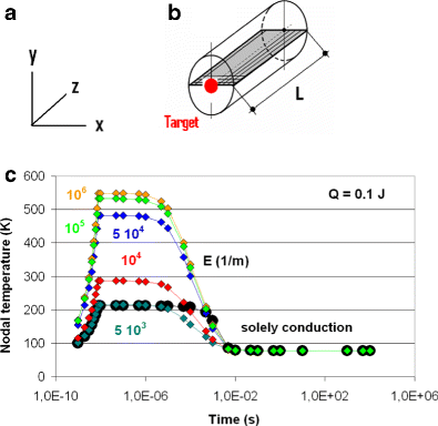
a, b Co-ordinate system and YBaCuO filament (schematic); the filament is exposed to a thermal disturbance (case (i), compare text), a single heat pulse of Q= 0.1 mJ deposited during 8 ns in the target plane (red circle, 0 ≤r≤r Target, z= 0). The shaded area containing plane finite elements is rotated around the symmetry ( z) axis (thin dotted line) to generate concentric cylindrical shells that constitute volume elements, for calculation of absorption and scattering. Orientation of the crystallographic c-axis of superconductor YBaCO material in this study was parallel to y-axis. c Nodal temperature at central front position ( x=y=z=0) of the YBaCuO filament. Temperature evolution is calculated by a combined finite element/Monte Carlo model that serves for solution of Fourier’s differential equation and for simulation of absorption/emission and scattering events, respectively. Data are given either for solely solid thermal conduction (solid black circles) or for conduction plus radiation heat transfer under different values of the extinction coefficient, E (solid coloured diamonds), respectively. The extinction coefficient is considered as independent of wavelength in the interval between about 20 and 100 μm (compare the explanations in [11])

Conductor temperature distribution may become highly inhomogeneous, with temperature variations in the conductor cross sections in the order of tens of Kelvin, and with corresponding impacts on critical current density and superconductor stability.
-
(ii)
Periodic disturbances [12]: exposure of a sample to periodic energy pulses
As local disturbances, they lead to periodic variations of local temperature and, correspondingly, periodic variations of critical current density and stability functions (Fig. 2).

a Orientation of crystallographic ab-plane and c-axis directions and of orthotropic thermal diffusivity components of YBaCuO with respect to overall ( x,y) coordinate system. Thick red solid lines assigned “ab” indicate direction of the (large) diffusivity in the crystallographic ab-planes, the much smaller diffusivity component parallel to the c-axis is represented by the blue line. b Stability function for periodic point-like disturbance (case (ii)) of DC transport in the 1G filament conductor calculated with the c-axis solid thermal diffusivity oriented parallel to the y-axis of the overall coordinate system (a, upper diagram), for rigorous solid conduction plus radiation and solely solid conduction (solid and open coloured diamonds, respectively). The disturbance is deposited in the red target plane (like in Fig. 1b), 0 ≤r≤r Target, y= 0. Results are given, at increasing axial distances (planes), y, from the target. The disturbance amounts to Q(t)= 2 Q 0 sin(2 π ω t)+Q 0 [W], with Q 0= 0.0125 W. Light and dark green, blue and black solid circles, introduced at t= 36, 67 and 106 ms, help to identify significant differences (advance in time) of about 30 and 39 ms, at y= 325 and 525 μm, respectively, by which the conductor, for stability function Φ= const, reacts earlier to a disturbance. The figure is taken from [12]
Like in case (i), conductor temperature and, accordingly, critical current and transport current density distribution become strongly inhomogeneous. The stability function is not constant but oscillates like the disturbance, and its shape varies with position, in axial direction, along the conductor (Fig. 2): times, t 1 and t 2, at which the stability function attains a constant value, for example, Φ= 0.4, differ by Δt 1,2 of about 30 ms, between axial positions y= 325 and 525 μm, respectively. This means magnitude of zero loss transport current will depend on time and on position.
2.2 Multi-filamentary Conductors
Cases (i) and (ii) in Section 2.1 apply single or oscillating disturbances under constant direct currents (DC). A very interesting case (iii) appears when density of an alternating current (AC) itself initiates periodic disturbances. The disturbances then are no longer point-like, isolated from each other or of only very short duration, but may be extended over the total superconductor cross section and exist during extended periods of time. As long as conductor temperature is below critical temperature, losses that result from this situation are flux flow losses.
Before we concentrate on stability analysis in a multi-filamentary, high-temperature superconductor, we shortly return to papers cited in [10] on quench analysis of large superconducting, LHe-cooled magnets. The analysis presented in [19, 20] assumes the conductor temperature (superconductor filaments plus copper matrix) as homogeneous so that in direction parallel to LHe flow, a 1D simulation of fluid, electrical and thermal transport is appropriate. The corresponding transport channels in the conductor (1D “chains”), after further simplifications (like homogeneous temperature also in steel jacket and insulation, but with temperature gradients in-between these components), finally are coupled to a 3D grid, by thermal convective and contact resistance, nodal links. Electrical and thermal properties of the materials involved, in particular their isotropy, favour application of this procedure and greatly simplify numerical computation.
Reasonable alternatives to [19, 20] for stability analysis in large, LHe-cooled magnets, which in particular would include approximate solution of the fluid flow equations, are hardly imaginable, at least from the point of presently available numerical tools and computing facilities. This is excellent work, but in high-temperature superconductors, the problems associated with inhomogeneous temperature fields remain.
The following finite element stability analysis is not focused on large devices like a superconducting magnet but on microscopic conductor geometry, in this paper a multi-filament, first-generation (1G) BSCCO 2223 high-temperature conductor (Fig. 3). But the numerical procedure could also be applied to any other superconductor material and conductor architecture.

Cross section of the 1G BSCCO 2223/Ag Long Island superconductor (above, the figure is taken from (21)), and finite element model cross section (present work, below) that schematically shows filaments (black) and matrix material (Ag, light grey). The crystallographic c-axis is vertical to the filament planes. All superconductor materials parameters used in the finite element calculations (thermal diffusivity, critical temperature and current density, critical magnetic field, anisotropy, weak link behaviour) are random values scattered around their nominal values (to take into account imperfections in materials development, manufacture and during handling of the sensitive 1G conductors). The Meissner effect is checked individually in each of the finite elements. Thin white lines indicate finite element mesh. Dimensions of filaments and of multi-filamentary conductor in x (horizontal) and y (vertical) directions are as follows: x= 280 µm (filament) and 3.84 mm (total conductor width), and y= 20 μm (filament) and 264 μm (total conductor thickness), respectively
The simulations apply a finite element programme (Ansys 16) that is embedded in a general simulation scheme conceived by the author. A disturbance is initiated by a sudden increase of (nominal) transport current in an electrical circuit.
For description of the stability problem, overall dimension of the electrical circuit is of little importance. We could in principle take any large- or small-scale electrical grid, like in a laboratory experiment, with an appropriately dimensioned superconducting component; the point is the analysis of this component under high current load.
In contrast to [19, 20], the stability analysis is focused on electrical and thermal transport in a single conductor within its filaments and its Ag-matrix material, to improve understanding of the physics behind superconductor stability:
-
(a)
Longitudinal current transport (parallel to coolant) is modelled like in [19, 20] but (instantaneous) transverse current distribution, calculated in small time steps, follows from application of Kirchhoff’s law. The calculation incorporates both superconductor and matrix elements in planes located at several longitudinal positions; the planes are perpendicular to overall current flow, and in each plane, total transport current (including current shared with the matrix) is conserved,
-
(b)
Longitudinal and transversal thermal transport and the resulting temperature distribution are calculated in a global 3D finite element scheme covering the total cross section, not by coupling 1D solutions by thermal convective and contact nodal resistances to a 3D scheme.
-
(c)
Both flux flow losses, and Joule heating also in the Ag-matrix material, are accounted for in the present analysis. Current sharing is possible if resistance of the matrix material becomes less than the resistance of the superconductor, which may occur either in case of flux flow or Ohmic conductor resistance.
In order to study the effect of flux flow on temperature distribution in the superconductor, a divisor, N Cutoff, is applied to total AC resistance of the simulated electrical circuit, beginning like in [18, 22] at t= 6.5 ms after start of the simulation with N Cutoff= 1. The divisor in the following increases gradually from its initial value to the final N Cutoff= 20 at t= 9 ms, and then is kept constant. The variation of N Cutoff simulates a strong disturbance.
Results of the simulations are shown in Fig. 4a, b. Temperature distributions in the conductor again are strongly inhomogeneous. Inhomogeneity, even in the tiny filaments, arises already before conductor temperature exceeds critical temperature (Fig. 4a), at any position in the cross section.

Temperature field (nodal temperatures) in the cross section of the BSCCO 2223 multi-filamentary conductor (Fig. 3; because of symmetry, only the left half of total conductor cross section needs to be shown, and symmetry axis is on the right). Results are observed at a t= 8.3 ms (top, with all temperatures below critical temperature, T Crit= 108 K at zero magnetic field) and b at t= 8.6 ms (bottom), respectively (1.8 and 2.1 ms after start of a permanent disturbance initiated by a large fault current). The disturbance results from a sudden increase, within 2.5 ms, beginning at t= 6.5 ms, of AC transport current to a multiple of 20 times its nominal value. Local temperatures are identified by the corresponding horizontal bars. Symbols MX and MN indicate positions in the cross section where minimum and maximum temperature is observed. b is taken from [22]. Temperature in the upper half of (a) and (b) is larger than in their lower half cross sections; in this example of field orientation, magnetic flux density arising at the Ag/filament interfaces in the upper half cross section is settled to exceed flux density in the corresponding lower half sections, which by reduction of J Crit initiates non-zero flux flow resistances in the (upper) regions. Transport and fault over-currents thus preferentially occupy the lower half of the cross sections
In Fig. 4b, only tiny parts of the individual cross sections have become normal conducting (hot spots generated at these positions) while most of the conductor cross section remains at temperature below critical temperature, T Crit. Current limitation, if any, accordingly would rely on Ohmic resistance in only these parts of the filament while in the remaining parts, zero resistance or flux flow resistance would co-exist, side by side. If the disturbance by a fault current is continuous, at least during 100 ms, and both redistribution of losses in the conductor volume and transfer to coolant is insufficient, conductor temperature in all parts of the cross section will increase steadily but temperature inhomogeneity will remain.
Accordingly, the point is that the mechanism (purely flux flow or Ohmic resistance) that would trigger switching the over-current to a shunt cannot uniquely be identified. The same applies to current limiters operating without shunt (these were the first concepts of fault current limiters). Inhomogeneity of conductor temperature neither allows to definitely identify the limitation mechanism (Ohmic, flux flow?) nor the achievable limitation factor and the time of onset of current limitation or of current sharing.
Besides imbalances between generated local losses and redistribution (thermalisation) of these losses within conductor volume and to the coolant, inhomogeneity of temperature distribution in cases (i) to (iii) results also from strong anisotropic thermal diffusivity: parallel to c-axis, towards the solid/coolant interface, diffusivity in BSSCO 2223 is about a factor 60 to 100 smaller than in the crystallographic ab-plane, see later. Characteristic time, τ Th, for conduction heat transfer thus is in the order of 0.6 ms, much larger than in the other directions. AC voltage and, accordingly, AC losses under frequency ω= 50 Hz become zero at t= 10 ms, but even if losses would be set to zero for all t >10 ms, recovery from the strongly inhomogeneous temperature distributions in Fig. 4a, b to below T Crit would not be achieved before hundred milliseconds, as a consequence of the large anisotropy ratio of the diffusivity. This period would be too long for technical applications.
The temperature distributions shown in Fig. 4a, b must be reflected by the distribution of critical and of transport current density (in zero-loss situations, transport current density exactly reflects critical transport current density). Spatial distribution of the obtained temperature field, T(x,y), of the flux flow resistivity, ρ FF(x,y) and of transport current, I(x,y) in the cross sections, all at the same time, t= 8.3 ms, is shown in Fig. 5a–c (the figure is taken from [22]). Flux flow resistances exist in parallel to Ohmic resistances (location of Ohmic resistances, not given in Fig. 5b, can be identified from Fig. 4a, b). Transport current obviously prefers regions of low temperature and avoids regions of increased resistance.

Distribution of conductor temperature (top), flux flow resistivity, ρ FF (below), and of transport (fault) current, I (bottom of the figure), in the x,y-cross section (Fig. 3) of the multi-filamentary BSCCO 2223 conductor. Like in Fig. 4a, b, only the left half of the cross section, x≤ 1.92 mm, y ≤ 264 μm, is shown. Results are presented at t= 8.3 ms (1.8 ms after start of the disturbance). Flux flow resistivity ρ FF >0 exists only if transport current density exceeds critical current density, J Transp > J Crit, and if local conductor temperature, T(x,y,t), is below local critical temperature. The figure is taken from [22]. Transport current avoids regions of increased resistance
The results shown in Fig. 4a, b and 5a–c rely on a variety of parameters of which flux flow resistivity is one of the most important. How can flux flow resistivity be calculated? This will be addressed in Section 3.
3 Finite Element Treatment of Flux Flow Resistance
3.1 Survey
A finite element mesh with fine spatial resolution has to be constructed for the conductor cross section shown in Fig. 3. But conductor dimensions are between nanometres (weak link structures), micrometres (grains) and millimetres (filaments and overall dimension of the multi-filamentary conductor). Mapping each superconductor grain, and in particular its surface, with at least some tens of appropriate elements (even a conservative approach) inevitably leads to a total element number of nodes and elements too large to obtain results within acceptable computation time.
Simulation of only substructures of the multi-filamentary conductor, like only 1 or 2 of the 91 filaments in Fig. 3, certainly would reduce computation time, but it would not be very helpful for temperature and current distribution and for stability analysis: we need simulation of the total number of filaments in the conductor, because it is the surface of the conductor, not of the filaments, that faces the coolant. Only the distribution of disturbances in all filaments, and the corresponding local losses, will in sufficient detail provide the temperature field in the total conductor cross section and qualify predictions of conductor stability as reliable.
Instead, calculation of an effective resistivity, ρ eff, of filaments, by application of a cell model, as an average taken over all relevant superconductor filament components, presently appears to be a manageable way. This step circumvents the problem that would arise from detailed mapping. A series of approximations (steps 1 to 4) will be necessary, and is described below.
Application of the cell model is restricted to the level before start of the proper finite element simulations. The effective resistivity, ρ eff, is applied in the finite element solution procedure as if the filaments were a continuum. The total numerical procedure thus is a continuum approach, like the finite element simulations in [18] and [22], in the present paper with improved spatial resolution.
3.2 Standard Model for Calculation of Flux Flow Resistance
In the low-temperature limit, the empirical relation between the specific resistivity, ρ FF, initiated by flux flow to current transport and, ρ NC, of normal conducting state reads as follows:
See [23], p. 230, and the cited reference to original literature, or compare other standard volumes on superconductivity. It has been shown that this relation is applicable to also high-temperature superconductors [24].
In (3a), the resistivity, ρ NC, usually is considered the room temperature (constant) normal conduction value of the superconductor solid material. However, the simple (3a) is valid for homogeneous superconductor solids, and it is also not clear that ρ NC should be kept constant in calculations of flux flow resistivity. In particular, (3a) without modifications does not appear to appropriately include weak links between solid constituents (grains, domains) in microporous conductors as they might contain a variety of different structure (1D to 3D geometry) and materials composition that each contribute to electrical resistance. Further, as [25], p. 128, indicates, there may be deviations from (3a) in type II superconductors, like YBaCuO or BSCCO, with large values of the Ginzburg-Landau parameter, but this will not be considered here.
Direct experimental determination of ρ FF would be difficult, not only because flux creep, a competition to flux flow operating in the background and of different origin that inevitably raises with increasing temperature.
The idea to extract flux flow resistivity from the slope of the I/V or J/E-curves performed in [24] with YBaCuO low-angle tilt grain boundaries basically appears to be reasonable, and the measurements are straightforward. But when the field was perpendicular to the ab-plane, the authors assumed the vortices were pinned by dislocations. Pinning of vortices in high-temperature superconductors (because of their large anisotropy of current transport and of field penetration) neither can be limited to an atomistic structural view (like dislocations) nor do pinned vortices reflect the comparatively simple geometrical structures (flux lines, vortices) found in low-temperature (metallic) superconductors. Instead, flux lines or vortices may strongly be distorted from external field direction and, depending on temperature and magnetic field, may be twisted.
3.3 Modelling of Weak Links
Weak links, on the one hand (and on a nanoscopic scale), exist as electrically insulating inter-layers between neighbouring crystallographic ab-planes, which means as natural Josephson junctions, or weak links appear, on microscopic dimensions, as 3D materials “bridges” between neighbouring grains and domains (in high-temperature superconductors of good quality, as clusters of orthorhombic, parallel oriented grains). There are also weak links consisting of 2D interfacial or 1D point contacts only.
In general, two paths are open to current transport through a particle bed, like in a multi-filamentary conductor: the conductor is composed of superconductor particles and empty or filled voids. In powder in tube (PIT) conductors, voids might partly be filled with Ag-matrix or with weak link material, or the voids result from pores that result from materials or manufacture imperfections and are simply filled with air. Currents paths are described as follows:
-
(a)
Intra-granular currents that in the Meissner state, as zero loss displacement and screening currents, yield zero internal magnetic field.
-
(b)
Inter-granular currents flowing through 3D, 2D and 1D contacts between neighbouring particles and multiples thereof; these currents not necessarily would be zero loss currents. Inter-grain paths are of practical importance.
Either path can be assigned a corresponding resistivity. A total, effective resistivity, ρ eff, then integrates all resistances opposed to intra- and inter-grain currents within an appropriately designed geometrical cell. We will use in (3a) and in the finite element simulations the ρ eff as a function of temperature instead of a constant ρ NC.
The dependence of ρ FF on magnetic field, given by the factor B/ B Crit2, is taken into account solely in the finite element procedure, with local flux density, B=B(x,y,t). The overall structure of (3a) then is conserved. Temperature dependency of both ρ eff and B Crit,2 has to be considered (the latter is considered also in [24], but is apparently often neglected).
An improved theory, still to be developed, might give up standard assumptions like a viscosity opposed to flow of flux quanta, and even suspend (3a), except for application to homogeneous solids. However, a practical way is to calculate ρ FF presently in a network composed of superconductor grains and domains and weak links in between.
It is assumed in the following that the domains are built by staples of a large number of plate-like single grains that during sample preparation in powder in tube processes are pressed to an ordered particle “bed” with the crystallographic ab-planes parallel to current flow (in Fig. 6a, in parallel to the x,z-plane, see below).

a Geometrical cell model for the calculation of the resistivity, ρ NC, to be applied in (3a), and in the finite element simulations as an effective resistivity, ρ eff. Above, the figure shows three arbitrarily selected filaments (schematic, no to scale; this is a detail of Fig. 3). Filaments are indicated by black rectangles (cross sections in a could be modelled with circular cross sections as well). Each filament (first detail, right, below) consists of a number M ×N domains (clusters of orthorhombic plate-like, parallel-oriented grains) each of which incorporate a superconductor core (large black rectangle) and a shell of weak link material (light grey). Each of the M ×N domains is divided into a number N=m×n grains (second detail, bottom part of the figure, left) each with again a superconductor core (small black rectangles) and a thin sub-shell of weak link material (white lines); this hierarchy of large and small superconductor cores in domains and grains and of correspondingly thick and thin shells and sub-shells facilitates modelling resistances of grains and weak link materials of different size, thickness, materials composition, physical properties and field dependence, respectively. See (c) for dimensions of domains and of grains and of the corresponding weak links sections. Total simulated conductor length, z, taken over large numbers of grains, domains and filaments is arbitrary. Numerical values indicating size of cross section of one filament are in micrometre. Resistances to current flow in z-direction of all domains and grains, filaments and Ag-matrix material are switched in parallel. The geometrical model assumes roughly layered grains and filaments. The multi-filament conductor in Fig. 3 incorporates 91 filaments. b Resistivity of BSCCO 2223: material properties, not including the effect of magnetic field. Red diamonds indicate experimental values reported in [30] for micro-crystalline BSCCO 2223. The reported porosity π1= 0.0842 (volume fraction 91.6 %) and the Russell cell model, in steps 1 to 2 (compare text), allow to extract the resistivity of the proper (ideal), solid grain core material, blue diamonds, inner porosity π2= 10 −4. In step 3 (the cell model now applied to the blue diamonds), the resistivity of the weak link materials enclosing domains and grains (porosity π3= 0.99 and 0.01, respectively) is estimated (light-green and light-blue diamonds, respectively; at T≥ 120 K, values of the anisotropy coefficient, r, are missing, but the light-green diamonds are extrapolated to this temperature range. The resistivity of the proper solid grain (bulk) material (blue diamonds), the proper solid, because of its almost zero porosity), necessarily must be smaller than the experimental resistivity (red diamonds) that refers to porous polycrystalline 2223 superconductor. c Flux flow resistivity, ρ FF, calculated from the effective ρ eff (compare text) and with the field factor B/ B Crit,2 in (3a) to current transport of a multi-filamentary BSCCO 2223 conductor, for local (constant) magnetic flux density, B= 10 and 100 mT (solid dark-green and light-green diamonds, respectively). Dimensions of domains, x 1, y 1 and z 1, are 70, 6 and 70 µm, thicknesses dx 1,dy 1and dz 1 of weak link shells enclosing domains are 100, 10 and 100 nm, respectively. Dimensions of grains, x 2, y 2 and z 2,are 20, 1 and 20 µm, thicknesses dx 2,dy 2and dz 2of weak link shells surrounding grains are 1, 1 and 1 nm, respectively. Solid blue circles indicate ρ Grain as solely the grain core (bulk) material without magnetic field and under zero current (note the temperature range is reduced to 98 ≤T≤ 108 K). Open dark green diamonds denote ρ FF from [22] calculated with B= 10 mT. For comparison, dark-grey diamonds indicate resistivity of the Ag-matrix material. The upper critical magnetic field, at T= 4.2 K, is B Crit,20= 200 T giving B Crit,2(T)= B Crit,20[1 − (T/ T Crit)2]. Critical temperature (vertical, dashed red line, for B = 0 and under very small current) is 108 K
A corresponding model reported by [26] describes total current of a 2223 tape conductor through a network of parallel weak and “strong” links, with strong field dependence of critical current density, J Crit, in weak, but with dependence of J Crit on flux pinning, in strong links. Weak links in this model are regarded as Josephson junctions, and strong links are represented by the solid grain material. While separation with respect to field dependence of J Crit principally appears to be sound, we believe the assumption of parallel (which strictly speaking means, contactless) paths, like the imagination of separate “chains” (two current paths) would be too much an approximation to be successful. On the micro- and nanoscopic size level, grains and their weak links in reality are disorderly arranged; ordered structures become obvious not before grains are compressed to domains and to filaments, under thermo-mechanical treatment during PIT manufacture.
3.4 Flux Flow Resistance from a Cell Model
Instead of assuming separate chains (current paths), a better solution in a resistance network is to account for the interplay between weak and strong links by appropriate cell models. Different field dependency of weak links between neighbouring grains and domains then can be accounted for, and the resulting effective resistivity incorporates both geometry of grains, filaments and weak links and their material composition. But this is a difficult task, too.
In the cell approximation, we in the first step extract the resistivity of the proper (ideal, zero porosity) solid (bulk) material from measurements of the resistivity of a multi-filamentary, polycrystalline PIT conductor (that to all experience is not ideal at all). Applying the resistivity of simple bulk material is not recommended for this step: The material does not undergo the special mechanical and thermal treatments usually applied to PIT conductors. Instead, preparation of bulk material yield samples that are geometrically as well as structurally different from samples prepared in the PIT process that applies a tape encapsulated in a Ag-jacket.
Extraction will be made from the resistivity of BSCCO 2223; resistivity of this material is accessible from the literature. After the first step, with the same cell model, the extracted resistivity is converted to the resistivity of weak link material, resident on the periphery of grains and domains.
A survey on cell models is given, for example, in [27], p. 7 to 15, and in [28]. The underlying Russell cell model [29] (see below, (3b)) is easy to handle since it just contains porosity and the resistivity of both (solid and porous) phases, either for electrical or thermal transport. It is flexible (the role of particles and voids without much effort can be interchanged), the results roughly are independent of size of the constituents, and though the model in its original scope applies to a regular distribution of cubic particles, it is according to experience applicable to particulates of also other shape and of modestly irregular spatial distribution. In the present case, for application of Russell’s cell model, the “particulates” are grains and domains distributed in a filament, and tiny voids of nanoscopic dimensions that represent weak links provided their geometry and material composition can adequately be indicated.
Small porosity in this picture indicates that weak links constitute only a small volume fraction in relation to the superconductor phases (grains, domains). The cell model does not assume particles or voids arranged in coherently connected, non-interacting chains. Instead, particles and voids are interpreted as distributed obstacles to current flow. The cell model treats all resistances that contribute to the (spatial) average ρ eff as if they would be randomly distributed. Calculation using the Russell or other cell models thus is straightforward, but the Russell cell model is particularly preferable when in the first step, the reverse of (3b) (see below) has to be used.
The conductor cross section (Fig. 3) is mapped upon a geometrical (schematic) model (Fig. 6a). The geometrical structure allows to assign each of its particular cross sections a specific resistivity (grains, domains, filaments and voids specifying weak links). These have to be calculated from repeated application of the Russell cell model, in a series of successive approximations, and for this purpose, all these have to be assigned a specific porosity.
3.5 Application of Russell’s Cell Model
Each of the 91 filaments in the multi-filamentary conductor (black rectangles in Fig. 3) is divided into M × N domains, and each domain in m × n grains (Fig. 6a). This implies division of the solid constituents of the filaments into a three-level hierarchy (“large” domains, “small” grains, “tiny” weak links) the benefit of which is to assign specific, position and field-dependent values of resistivity to each section of the whole filament. Each domain is composed of a solid core (the proper superconductor, black rectangles) and of “shells” (light-grey sections) that at the moment and only schematically indicate weak link materials arranged around the black cores. In the proper calculation of the effective resistivity, the shells’ cross sections are in z-direction reduced to point-like contacts (this shall be realised with the help of results from analogous thermal transport problems through particle beds, see Section 3.6). Each grain incorporates its own superconductor core (again black rectangles) and corresponding sub-shells (thin white lines, the weak links between grains). Electrical transport through the matrix material, of well-known resistivity, is accounted for solely in the finite element scheme.
Manufacture of 1G PIT filamentary conductors results in plate-like grains with dimensions x, y, z= 10, 1, 10 µm or also in needle-like particles of 10 to 30 µm length, with a diameter of about 1 µm. Range of grain size distribution may be wide, but results of the flux flow resistivity calculations differed only slightly between both plate-like or needle-like grain geometry; the present paper applies plate-like gain geometry. Size of domains increases with number of grains but remains in the micrometre range, thickness of corresponding shell and sub-shell, weak link materials are in the order of one to tens of nanometre. Dimensions are given in the caption of Fig. 6c; with these dimensions, shell volumes in Fig. 6a, even before reduction to point-like contacts, are much smaller, by a factor of about 400, than BSCCO superconductor (solid grain and domain) volumes.
Within the present geometry (Fig. 6a), principal porosity, π1, of superconductor components in the multi-filamentary conductor (91 filaments distributed in the Ag-matrix) is about 0.5 (related to total conductor volume). Though there are comparatively thick Ag-sections in Fig. 3a (left and right to the black filaments), the percentage of BSCCO is larger than frequently reported 30 to 40 % of BSCCO in OPIT BSCCO/Ag superconductors ( π1= 0.6 to 0.7). But the most important result (inhomogeneous temperature distribution) does not change if either principal porosity π1(0.5 in the present case, or 0.6 to 0.7 from literature) is applied in the simulations.
If k Core denotes thermal or electrical conductivity of solid particles that are completely embedded in a “shell” of conductivity, k Shell, the integral conductivity, k, in the Russell model of an open cell structure with porosity π reads as follows:
We apply (3b) to measured resistivity, ρ= 1/ k= 1/\(k_{{\exp }}\), with \(k_{{\exp }}\) from [30] (red diamonds in Fig. 6b) of a PIT conductor (grains and domains distributed in a Ag-matrix). The reported critical current density is 7 × 10⁸ A/m 2, and that the superconductor BSCCO 2223 core was prepared in solid-state reaction.
The measured \(k_{{\exp }}\) then are converted to the resistivity of a corresponding ideal, almost zero porosity solid (core) grain material (like a basis vector from which solids or porous structures of any porosity can be derived). Probably existing contributions from BSCCO phases other than 2223 and weak link materials are included in the red diamonds. This is step 1: Russell’s (3b), with the principal porosity π=π1=0.084 given in [30], has to be solved for k Core.
For this step, the conductivity k Shell has to be defined. We roughly assume k Shell≈ 1/100 \(k_{{\exp }}\). In BSCCO 2223, the factor 1/100 reflects experimentally determined anisotropy of thermal conductivity. The anisotropy ratio r(T)=λ ab(T)/ λ c(T), of thermal conductivity, λ, approximately may be considered as also the anisotropy of current flow or of field penetration. The idea is that electrical resistivity of superconductor components in weak links, if they are at least partly composed of the BSCCO 2223 phase (or of other phases of approximately the same anisotropy ratio), hardly will be larger than resistivity against current transport in c-axis direction between neighbouring ab-planes in the crystallographic unit cells.
If ab-planes in crystallites or grains in the weak link material are randomly (but with small tilt angles) oriented against current flow, the resistivity, ρ Shell(T), then would be smaller than \(\rho _{{\exp }}(T) r(T)\) which means application of k Shell= 1/ ρ Shell(T)= 1/[\(\rho _{{\exp }}(T) r(T)\)] in (3b) yields an underestimate of total k, or an overestimate ρ Core(T)= 1/k. This happens in step 1 and in all following steps that apply (3b). Because of the small percentage of shell volumes in the total cross section, uncertainty arising from overestimate of ρ Core(T) will at least partly be compensated. Experimental ratios r(T) using bare core material of a BSCCO 2223 PIT conductor, after removal of the Ag-jacket, are shown in Appendix A2 (Fig. 8).
In step 2, the result is transformed, again by (3b), to the resistivity of a real solid of non-zero (but very small) porosity, say for example, π2=πCore= 10 −4. This small correction (blue diamonds in Fig. 6b) assures that the structural composition (no voids) of the basic core material is almost perfect and consists solely of the BSCCO 2223 phase (voids originally resident in the red diamonds are eliminated in step 1). As mentioned, the blue diamonds not necessarily represent the resistivity of ordinary bulk material: the red diamonds in Fig. 6b apply to the bare core of the filaments that are prepared in a PIT process. Preparation of bulk material instead yields samples of clearly different mechanical and current transport properties.
In step 3, the blue diamonds in Fig. 6b shall be converted to resistivity of weak link material, again by application of (3b), but now with much larger (see below) shell porosity, π3=πShell. In this case, large porosity means that the solid component, now of the weak link material, contributes only marginally to resistance of weak links.
Micro- or nanoscopic metallurgical sections or SEM pictures are not available the resolution of which would allow more than just getting very rough impressions of spatial structure and porosity of 3D weak link materials. Also, the tiny dimensions of weak links cannot be concluded from experiments. Weak links in addition might even consist of only 2D interfacial or 1D point-like contacts.
In a qualitative view, porosity πShell of weak link materials between domains probably is much larger than the corresponding πShell of weak links between grains, and porosity will increase with radial distance from position of inner-lying grains. This is because manufacture of PIT superconductors is subject to robust thermo-mechanical treatments; the conductors experience large frictional (from thermal expansion, winding) and compressive forces, the latter due to mechanical shock treatment (forging, down-hammering, rolling). Though the superconductor material is very hard, the very first ”receiver” of compressive and frictional load is the domain periphery, so that particle surfaces at these positions, in very thin surface layers, may be ground to almost a powder, in contrast to grains located (and thus mechanically protected) in the deep interior. Weak links between grains thus would contribute stronger to mechanical stability of the bed, in parallel to the matrix jacket, than weak links between domains. Assigning large πShell (close to 1) to domain weak links simultaneously assumes that the corresponding weak links are poor phases, in the proper BSCCO 2223 material.
As before, values of πShell of weak links between grains can be estimated only but this material would be rich in the superconductor phase. Whether in a melt the periphery of grains and domains is sharply defined depending on surface tension and decay rate of temperature, but we can expect that concentration of the proper superconductor material does not sharply break down to almost zero at the periphery; a finite concentration gradient is more probable.
Sensitivity analysis performed with a variation of 0.1 ≤πShell≤ 0.5 of shells around grains shows that ρ eff does not depend very strongly on πShell. Again, a merely qualitative view suggests that πShell of grains should be very small; thus πShell= 0.01 for weak links interconnecting grains was finally chosen, which means the BSCCO 2223 phase contributes almost exclusively to the grain weak links (contrary to weak links interconnecting domains). Experiments are needed to confirm these expectations.
But other BSCCO superconductor phases (compare Appendix A1) and probably existing contaminations may contribute to the resistivity of weak links, in different ways, however. This has been accounted for by separation of weak link resistivity according to magnetic field dependence: the resistivity from step 3 is in step 4 split into the proper field-dependent BSCCO phase (which means, below its T < T Crit= 108 K) and in the other BSCCO phases that do not (or no longer, at elevated temperature) depend on magnetic field, and thus cannot contribute to ρ FF. Normal conducting “foreign” contributions (contaminations) to the resistivity of weak links have to be eliminated from ρ FF, too.
In weak links between neighbouring domains and grains, considerable potentials exist not only for variations of geometrical structure and porosity but also for internal materials composition, see Appendix A1.
Finally, the resistivity resulting from steps 1 to 4 is used to calculate resistances, R j (1 ≤j≤ 9, counting horizontally the light-grey and black cross sections within a grain or a domain in Fig. 6a). The R i in grains and domains are finally switched in parallel (in z-direction). The light-blue and light-green diamonds in Fig. 6b include only steps 1 and 2.
3.6 Thermal Analogue to Weak Links
After application of Russell’s cell model to estimate material properties in grain, domain and shell cross sections, the geometrical aspect of calculating the effective resistivity of the cell remains to be solved: shell cross sections (light-grey-shaded areas in Fig. 6a) have to be reduced to point-like contacts to represent weak links.
No experimental values are available on size or on number of electrical contacts and on their distribution on superconductor particle surfaces. Modelling of electrical resistance in particle beds originally goes back to Rayleigh and Maxwell and has been revisited more recently by Holm [31]. Kaganer [27] and several authors cited in this reference have converted the results from electrical transport to the analogous thermal transport problem. In turn, refinements achieved in heat flow-related studies can be used for solution of the present electrical transport problem in a two-phase medium (grains or domains, and weak links).
Figure 7 (schematic) shows a resistance cell unit between two spheres, with partial thermal or electrical resistances R 1 to R 4. The atomistic view in this figure reflects principles of cell models (as mentioned, the effective resistivity, ρ eff, finally is operated as a continuum approximation). Resistance 1 refers to solid material (for example, contacting spheres or fibres), resistance 2 contains a macroscopic contact area (2) with a size following from elastic deformation, and resistance 3 considers point contacts (3) within the contacting area (2). Point contacts in the thermal model arise from surface irregularities like roughness. Roughness either exists as natural surface roughness (a solely particle materials property) before contact, or it develops when contacting bodies are exposed to high pressure load or to thermal treatment (sintering, melting).

Thermal resistance units 1 to 4 between two spheres (schematic). Geometry of contact area, and dimensions of deformations are adapted from [33]. Resistances 1 to 4 may arise in thermal conduction problems or in electrical current flow and are identified as follows: 1 = solid material (for example, sphere or fibre), 2 = macroscopic contact area with size following from elastic deformation, 3 = point contacts arising from surface irregularities like roughness (weak links can be considered as a nano- to microscopic analogue of such irregularities in electrical current transport). Resistance 4 applies preferentially to thermal conduction and in this case causes a film resistance arising from condensation of a gas in the periphery of the macroscopic contact area; this is not considered here. The atomistic view in this figure reflects principles of cell models. The figure is taken from [32]
In electrical current transport, weak links can be considered the nano- to microscopic analogue of surface irregularities (3). For electrical contacts, Holm [31] has shown that the component R 2=R Cont in this figure is dominating among R 1 to R 3. By analogy, it is sufficient to apply for the electrical resistance R 3 (the resistance of weak links) the contact area (2); the procedure delivers an upper limit for R 3. It is thus R 2 that is used in the cell model to calculate resistance of weak links against current transport in z-direction through grains, domains and filaments.
Contact radii of the surface (2) in Fig. 7 for two touching spheres or fibres or for contacts between particles of other geometry can be estimated from Hertz’ theory for elastic or inelastic deformations; compare [27], p. 19, if pressure load, p, modulus of elasticity, Y, and Poison’s ratio, µ, are known. A constriction zone arising from deformation of contacting 3D bodies (spherical or of other geometry) ends in a 2D contact surface. Details are described in [27, 28] and [32] and in Appendix A2.
3.7 Results from the Cell Model
Summation of all R j obtained in the foregoing subsections, of all grains, domains and filaments, all switched in parallel, yields the total conductor resistance, R Total=ρ eff L/A, for current flow in z-direction, with L the length of the conductor and A its total cross section. This equation is solved for the effective resistivity, ρ eff, opposed to current flow in axial (z-) direction.
In Fig. 6c, flux flow resistivity, ρ FF, is calculated from the effective ρ eff (obtained in the cell model) by multiplication with the ratio B/ B Crit,2(T), using constant B= 10 and 100 mT. In the finite element calculations, B=B(x,y,t) will be applied instead, with really existing local temperature and local magnetic fields. Local flux density in the filaments, at the superconductor/Ag interface, is in the order of 1 ≤B≤ 10 mT, using transport current through the multi-filamentary conductor from the simulated electrical grid under a fault. Grain, domain and filament dimensions are indicated in the caption of this figure.
The resistivity ρ FF, for B= 1 and 10 mT, in Fig. 6c is larger than ρ Grain because weak links drive flux flow resistivity of grains and domains to values greater than the proper solid resistivity ( ρ Grain). For the given flux densities, the resistivity ρ FF is also larger than the ρ FF= 10 −6Ω m, a constant value used in [34], and it greatly exceeds the resistivity of the Ag-matrix material. There will be current-sharing between superconductor and matrix provided transport current density in the filaments exceeds critical current density, and temperature is below T Crit.
But the resistivity ρ FF at T < 98 K in Fig. 6c is much smaller than the result reported in [35]; they find ρ FF≈ 1.5 × 10 −3Ω m at T= 87 K in a single-filament BSCCO 2223 PIT tape. Contributions from the 2212-phase ( T Crit= 94 K) to resistivity, and perhaps more normal conducting components in the weak links, and the absence of an external magnetic field, could explain this discrepancy (we note at T= 87 K, the critical current density of a multi-filament BSCCO 2223 PIT tape in this reference was clearly below 10 8 A/m 2, a comparatively small value which could be explained by increased weak link resistivity from insufficient pinning). As is to be expected, also the resistivity reported for an unordered polycrystalline BSCCO 2223 sample exceed, at least by one order of magnitude, the results obtained in Fig. 6c: in [36], the authors find ρ FF≈3×10⁻³Ωm at temperature very close to T Crit (108 K) in DC field experiments with overlaid small AC ripples. But part of the material looks like needles (Fig. 1 in [36]), without any preferential ordering, which as a priori induces higher resistivity.
The model described in this paper differs from the weak link path model reported in [37] where differentiation between superconductor operational states is restricted to “superconducting” or “normal conducting” only. But flux flow, too a superconductor state (because T < T Crit), is also responsible for conductor resistance to electrical transport, under the conditions mentioned above. Instead, the present cell model not only allows flux flow per se but takes into account parameters like grain and weak link materials dimensions and compositions. However, the cell model still suffers from a series of critical approximations and missing experiments to determine porosity.
We recall that one of the main objectives of the present paper and of and [11, 12, 18, 22] was to demonstrate high temperature inhomogeneity in filaments and multi-filamentary conductors under disturbances. The main result, inhomogeneous temperature distribution in the conductor (compare Fig. 4a, b and corresponding figures in [18, 22]), does not change when instead of the values for flux flow resistivity (obtained from the cell model) the normal conduction resistivity of BSCCO 2223, ρ NC= 2.87 × 10 −5Ω m at T= 300 K, from [30], would inserted into the finite element scheme (the main result thus can comparatively simply be confirmed, one only needs finite element or finite differences computer programmes, even analytical estimates of temperature gradients might already be sufficient). Accordingly, all consequences for current distribution, conductor stability against quench and predictions concerning current limiting that originate from strong inhomogeneity of the temperature field are conserved when using ρ NC instead of ρ FF.
4 Integration Times in the Finite Element Calculations
4.1 Problems with Thermal Diffusivity
In standard stability analysis, besides a dependence on magnetic field, the variation d J Crit[ T(x,y,t > t 0)]/dt, of critical current density ( t 0 the time indicating start of the disturbance) is considered to closely follow the variation d T(x,y,t)/dt of local temperature in the superconductor. Local temperature, T(x,y,t), after a disturbance, reflects thermal transport properties, which means phonon and electron contributions to thermal conductivity and to specific heat. For transient analysis of stability or current limiting problems, a corresponding characteristic, thermal relaxation time, τ Th, is defined; it is as usual derived from the thermal diffusivity applied in Fourier’s differential equation. Local temperature in a superconductor can hardly be measured; what is usually measured is its surface temperature or the temperature of a cold head to which a superconductor sample is thermally connected (the question is how perfect such connections, or remote measurement of sample temperature by IR thermography, can be realised).
But J Crit[ T(x,y,t)] depends strongly on properties of the sample’s electron system. Electrons that contribute to superconductivity are largely decoupled from propagation of thermal waves, and reflect their own dynamic response to this or other specific excitations by a corresponding relaxation time, τ El. The lattice, i.e. its phonon spectrum, if excited, behave differently; coupling of both systems in the BCS model may even be infinitely weak. The characteristic time, τ El, for decay of electron pairs, the “electron aspect” of propagation of a disturbance, and subsequent recombination of excited electron states to a new dynamic equilibrium, at different temperature and carrier concentration, thus would be quite different from τ Th though the number of electrons coupled to Cooper pairs near critical temperature is comparatively small. Nevertheless, it is τ Th that as a function of total thermal diffusivity is usually applied in finite element calculations (total means: phonon plus electron contributions), and the stability function is calculated on this “phononic” basis.
In the same way, the normal/superconductor phase transition that in reality corresponds to solely the electron system during warm-up or cool-down periods traditionally is considered to occur at exactly a time, \(t^{\prime }\), when measured solid temperature, \(T(x,y,t^{\prime })\), coincides with critical temperature. In standard experiment, T Crit is determined from observation of an electrical field suddenly arising over the sample when transport current exceeds critical current, again a completely electron-based aspect while temperature measurement is based on phonon plus electron contributions to thermal transport. But it is not clear that during cool-down a previously normal conducting electron system, in any of the superconductor volume elements, already had completed its return to a new dynamic equilibrium mixture of normal conducting and superconducting electron components in this volume, at the lower temperature and at exactly this time, \(t^{\prime }\). Thermal diffusivity usually applied in finite element calculations thus might contain contributions from super- and normal conducting electrons that have not yet returned to dynamic equilibrium. The finite element programme does not know the “history” of the total phonon plus electron system under a temperature variation. Uncertainty of results obtained from finite element calculation thus is unavoidable, not from computational but from physical aspects though such uncertainties might be small (but this is not clear). Uncertainty of this kind may become critical when temperature distribution in the conductor is not homogeneous.
Characteristic (relaxation or life-) times, τ El,of thermally excited electron states were numerically calculated in [38] from their decay rates using a sequential model with contributions (a) from a formal analogy to an aspect of the nucleon-nucleon, pion-mediated Yukawa interaction, (b) from the Racah-problem (expansion of an anti-symmetric N-particle wave function from a N− 1 parent state; this aspect is to be observed in summations of individual decay widths to total lifetime, τ El, of the excited electron system), and (c) from the uncertainty principle.
4.2 Time-Steps Applied in the Finite Element Calculations
Different characteristic (relaxation or life-) times, τ El, τ Th and τ B (the latter for propagation of magnetic flux at T > T Crit in a multi-filamentary superconductor) accordingly have to be taken into account in the numerical simulations: below T Crit, the electron system, after a temperature variation, must be given sufficient time to complete the said re-organisation before a new local temperature should be calculated. Time steps, Δt or, as in [12, 18, 22], the large number of iteration sub-steps of variable length within each Δt, for which the solution of Fourier’s differential equation shall be solved, accordingly must be larger than characteristic times τ El and τ Th. The proper integration time, δ t, within each sub-step Δt/ N≥ 10 −5 s, is between 10 −14 and 10 −7 s; convergence shall be achieved with these δ t at the end of each sub-step. The situation is relaxed only at temperatures above T Crit.
Multi-physics elements for appropriately handling the coupled superconductor electrical/magnetic/thermal conductive/radiative transport problems in finite element calculations, and in particular the re-organisation problem of electron states, are not available, and this situation will certainly remain in near future. Collisions between time-steps Δt (or their sub-steps) and τ El thus may arise, in particular if local conductor temperature is below but very close to critical temperature; there, τ El becomes large (compare Fig. 2a, b in [38]); re-organisation of the total electron state takes longer the larger the number of electrons involved. Analytic or finite element calculations performed with time steps chosen solely in relation to thermal diffusivity and element size but that do not observe conformity with the characteristic times τ El, τ Th and τ B may deliver questionable results although the achieved numerical convergence might be excellent.
There is also a spatial aspect to be observed in finite element calculations that involve superconductors exposed to magnetic field. Strictly speaking, local field in (3a) has to be taken as an average over the Ginzburg-Landau coherence length; nodal distances within the finite element mesh must be large enough not to collide with this condition. This in turn requests reconsideration of the proper integration time steps δ t.
5 Conclusions and Outlook
Under transient or permanent load, analysis of current transport in a multi-filamentary superconductor, including the stability and current limiting problems, requires simulations with high spatial and time resolution, with time-steps that are conform with three different characteristic times, τ El, τ Th and τ B. Analytic or finite element calculations that do not observe this conformity might deliver results that have limited correspondence to reality although numerical convergence might be fine. Superconductor temperature is not homogeneous, even in the tiny filaments in a multi-filamentary conductor. Clear distinction between purely Ohmic or flux flow resistance thus is not possible. Contrary to what is frequently reported in the literature, differentiation between corresponding flux flow or Ohmic resistance-type fault current limiters, or between corresponding triggering mechanisms to initiate current sharing, becomes highly questionable. A cell model calculation of flux flow resistivity has been presented in this paper that as an approach appears to be suitable for application in finite element calculations of temperature fields and current distribution in superconductors. But a variety of uncertainties arising with parameters selection is obvious, like in many numerical simulations. The model could perhaps be refined by adopting an idea of the weak link path model, i.e. a random distribution of weak link interfacial and “bridge” contacts on grains and domains. While (3a) applies well to solid superconductors, a cardinal rectification, strictly speaking, could perhaps be obtained when a new theoretical model is conceived without reference to normal resistance or viscosity in micro-porous conductors. More investigations will also be required to find a perhaps existing but still not identified, correlation between stability functions and current percolation.
References
Giese, R.F., Runde, M.: Fault-current limiters, In: Implementing agreement for a co-operative programme for assessing the impacts of high-temperature superconductivity on the electric power sector, Argonne National Lab., Argonne, Illinois, USA (1991)
Giese, R. F.: Fault-current limiters—a second look, in: Implementing agreement for a co-operative programme for assessing the impacts of high-temperature superconductivity on the electric power sector, Argonne National Lab., Argonne, Illinois, USA, (March 1995) (1995)
Kalsi, Sw. S.: Applications of high temperature superconductors to electric power equipment, pp 173–217. IEEE Press, John Wiley & Sons, Inc. Publ., Hoboken, New Jersey (2011)
Wilson, M. N.: Superconducting magnets. In: Scurlock, R.G. (ed.) Monographs on cryogenics, Oxford University Press, New York, reprinted paperback (1989)
Dresner, L.: Stability of superconductors. In: Wolf, St. (ed.) Selected topics in superconductivity, Plenum Press, New York (1995)
Blatt, J. M.: Theory of superconductivity. Academic Press, New York and London (1964)
de Gennes, P. G.: Superconductivity of metals and alloys. W. A. Benjamin, Inc., New York and Amsterdam (1966)
Tinkham, M.: Introduction to superconductivity, reprinted Ed., Robert E. Krieger Publ. Co., Malabar, Florida (1980)
Orlando, T.P., Delin, K.A.: Foundations of applied superconductivity, Addison-Wesley Publ. Comp. Inc., Reading, Mass (1991)
Seeger, B. (ed.): Handbook of applied superconductivity, Vol. 1, Institute of Physics Publishing, Bristol and Philadelphia, IOP Publishing Ltd (1998)
Reiss, H.: Radiation heat transfer and its impact on stability against quench of a superconductor. J. Supercond. Nov. Magn. 25, 339–350 (2012)
Reiss, H., Troitsky, O.Y.: Superconductor stability revisited: Impacts from coupled conductive and thermal radiative transfer in the solid. J. Supercond. Nov. Magn. 27, 717–734 (2014)
Flik, M.L., Tien, C.L.: Intrinsic thermal stability of anisotropic thin-film superconductors. ASME Winter Ann. Meeting, Chikago, IL, Nov. 29–Dec. 2 (1988)
Abeln, A., Klemt, E., Reiss, H.: Stability considerations for design of a high temperature superconductor. Cryogenics 32(3), 269–278 (1992)
Reiss, H.: An approach to the dynamic stability of high-temperature superconductors. High Temp.-High Pressures 25, 135–159 (1993)
Wetzko, M., Zahn, M., Reiss, H.: Current sharing and stability in a Bi-2223/Ag high temperature superconductor. Cryogenics 35(6), 375–386 (1995)
Reiss, H.: Simulation of thermal conduction and boiling heat transfer and their impact on the stability of high-temperature superconductors. High Temp.-High Pressures 29, 453–460 (1997)
Reiss, H.: Superconductor stability against quench and its correlation with current propagation and limiting. Journal of Superconductivity and Novel Magnetism 28, 2979–2999 (2015)
Bottura, L., Zienkiewicz, O.C.: Quench analysis of large superconducting magnets, part I: model description. Cryogenics 32(7), 659–667 (1992)
Bottura, L., Zienkiewicz, O. C.: Quench analysis of large superconducting magnets, part II: model validation and application. 32 8, 719–728 (1992)
Marzahn, E.: Supraleitende Kabelsysteme, Lecture (in German) given at the 2nd Braunschweiger Supraleiter Seminar, Technical University of Braunschweig (Germany). https://www.tu-braunschweig.de/Medien-DB/iot/s-k.pdf(2007)
Reiss, H.: Inhomogeneous temperature fields, current distribution, stability and heat transfer in superconductor 1G multi-filaments, accepted for publication by Journal of Superconductivity and Novel Magnetism. 10.1007/s10948-016-3418-1 (2016)
Tilley, D. R., Tilley, J.: Superfluidity and superconductivity, 2nd Ed., Graduate student series in physics, Adam Hilger Ltd., Bristol and Boston (1986)
Diaz, A., Mechin, L., Berghuis, P., Evetts, J.E.: Observation of viscous flow in YBa 2Cu 3 O 7−δ low-angle grain boundaries. Phys. Rev. B 58(6), R2960–R2963 (1998)
Huebener, R. P.: Magnetic flux structures in superconductors, Springer Series in Solid State Sciences, Vol. 6. Springer-Verlag, Berlin (1979)
Van der Laan, D.C., van Eck, H. J.N., ten Haken, B., Schwartz, J., ten Kate, H.H.J.: Temperature and magnetic field dependence of the critical current of Bi 2Sr 2Ca 2Cu 3 O x tape conductors. IEEE Transacts. Appl. Supercond. 11(1), 3345–3348 (2001)
Kaganer, M. G.: Thermal insulation in cryogenic engineering, Israel Progr. Sci. Transl., Jerusalem (1969)
Reiss, H.: Strahlungstransport in dispersen nichttransparenten Medien, Thesis for Habilitation, University of Wuerzburg, Wuerzburg, Germany (1985). http://nbn-resolving.de/urn/resolver.pl?urn:nbn:de:bvb:20-opus-66669
Russell, H.W.: Principles of heat flow in porous insulators. J. Am. Ceram. Soc. 18, 1–5 (1935)
Khan, M.N., Zakaullah, K.H.: Novel techniques for characterization and kinetics studies of Bi-2223 conductors. J. Res. (Science) 17(1), 59–72 (2006)
Holm, R.: Electric contacts. Springer Verlag, Berlin, Heidelberg (1967)
Reiss, H.: Radiative transfer in nontransparent, dispersed media, Springer Tracts in Modern Physics 113, Springer Verlag (1988)
Landau, L. D., Lifschitz, E.M.: Lehrbuch der Theoretischen Physik, Vol. III Elastizitätstheorie, in German. Akademie Verlag, Berlin (1965)
Shimizu, H., Yokomizu, Y., Goto, M., Matsumuara, T., Murayama, N.: A study on required volume of superconducting element for flux flow resistance type fault current limiter. IEEE Transacts. Appl. Supercond. 13, 2052–2055 (2003)
Cha, Y.S., Seol, S.Y., Evans, D.J., Hull, J.R.: Flux flow resistivity of three high-temperature superconductors, presented at the 1996 Appl. Supercond. Conf., Pittsburg, August 25 - 30, 1996, and publ. in IEEE Transacts. Appl. Supercond (1996)
Vanderbemden, P.H., Destombes, C.H., Cloots, R., Ausloos, M.: Magnetic flux penetration and creep in BSSCO-2223 composite ceramics. Supercond. Sci. Technol. 11(1), 94–100 (1998)
Ogawa, K., Osamura, K., Matsumoto, K.: Analysis of I-V Characteristics in Ag/Bi2223 tapes by weak link path model, CP614, Adv. Cryog. Eng., Proc. Intern. Cryog. Mat. Conf. - ICMC, Vol. 48, ed. B. Balachandran et al., Copyright Amer. Inst. Phys., 1102–1109 (2002)
Reiss, H.: A microscopic model of superconductor stability. J. Supercond. Nov. Magn. 26(3), 593–617 (2013)
Hao, Zh., Clem, J. R.: Viscous flow motion in anisotropic type-II superconductors in low fields. IEEE Transacts. Magn. 27, 1086–1088 (1991)
Aubele, A. C.: Phasengleichgewichte im System Bi 2 O 3-PbO-SrO-CaO- CuO-Ag, Doctoral Thesis (in German), Max Planck Institut für Metallforschung; University of Stuttgart, Stuttgart, Germany (2002)
Fricke, J., Frank, R., Altmann, H.: Wärmetransport in anisotropen supraleitenden Dünnschichtsystemen, Report E 21 - 0394 - (1994). In: Knaak,W., Klemt, E., Sommer, M., Abeln, A., Reiss, H. Entwicklung von wechselstromtauglichen Supraleitern mit hohen Übergangstemperaturen für die Energietechnik, Bundesministerium für Forschung und Technologie, Forschungsvorhaben 13 N 5610 A, Abschlußbericht Asea Brown Boveri AG, Forschungszentrum Heidelberg, (1994)
Cahill, D. G.: Thermal conductivity measurement from 30 to 750 K: the 3ω method. Rev. Sci. Instrum. 61(2), 802–808 (1990)
Gherardi, L., Caracino, P., Coletta, G.: Mechanical properties of Bi-2223 tapes. Cyrogenics 34(1), 781–784 (1994). ICEC Supplement
Laubitz, M.J.: Thermal conductivity of powders. Can. J. Phys. 37, 798–808 (1959)
Author information
Authors and Affiliations
Corresponding author
Appendices
Appendix A1 Material Composition of Weak Links
Microporous materials of any kind inevitably contain weak links. They constitute obstacles, at least against the following:
-
(i)
Electrical transport (Ohmic resistance to flow of electron charges)
-
(ii)
Magnetic transport (movement of vortices under flux flow)
-
(iii)
Thermal transport (propagation of lattice excitations), and even against fluid transport, if any is involved
Electrical resistance calculations to items (i) and (iii) are straightforward; a very large number of experimental data exists. The proper problem concerns item (ii) in case it is not a homogeneous solid but a micro-porous superconductor the flux flow resistivity of which has to be determined.
In the finite element calculations, as described in the text, this problem is tentatively circumvented by calculation of an effective resistivity, ρ eff, by application of a cell model. Weak links between grains and domains built up from crystallites and grains are electrically conducting or insulating, which means they can be composed of superconductor and of normal conductor components or of contaminations.
Because of the small coherence length, weak link geometry in high temperature superconductors ranges from Josephson junctions with nanoscopic dimensions to solid bridges of finite, but tiny volume; all of these form a network of resistances to current flow and most of them are related to materials manufacture. Different crystalline and amorphous structures, variations between low to large angle tilt grain boundaries, twist boundaries and different textures, may contribute to electrical resistances within grains and contacts between grains; among these, low-angle tilt grain boundaries may be considered as (relatively) “strong” links (essentially, these are the superconductor grains). Results for critical current density reported in [36] may be the consequence of “current sharing”, here not between superconductor grains and matrix material, but between said strong links and current paths via tiny spatial or interfacial or contact weak links.
Besides spatial (contact) inhomogeneity of weak links, there are also variations of material composition, like in grains. Variations of materials properties in grains comprise mixtures of residual 2212 and 2223 phases of the BSCCO family (the 2223 phase emanates during solid-state reaction from the 2212 phase). This means relative contributions from different phases depend on temperature, length of sintering steps and their repetitions, and on phase stabilising measures like Pb doping to achieve high stability of the 2223 phase (and to reduce synthesis temperature). There is also strong anisotropy of flux flow not only in grains but also in grain boundaries [39], much larger than the anisotropy of resistance to standard current transport.
More variations of grain materials properties result from different oxygen contents, different additions like Sr, as well as from presence of the BSCCO 2201 phase. The 2223 phase is surrounded by a manifold of undesired Bi-, Pb- and Cu-containing phases; their relative contribution by volume is about 10 % [40]. It is hardly possible to obtain a one-phase 2223 in PIT industrial conductor manufacture. But under the superconducting secondary phases, the 2212 is dominating, at low enough temperature.
Bi-containing phases other than BSCCO 2223, like 2201, 2212 and 2234, have T Crit= 13, 94 and 104 K, respectively. Since it is difficult to synthesise the 2234 phase, it will hardly appear, neither as a grain nor as a possible weak link component, which means, at T≥ 77 K, probably the only competitor to 2223 precipitation in grain and weak link materials is the phase 2212. But at given working core temperature, T > 94 K, still below the T Crit= 108 K of the 2223 phase, the T Crit of the 2212 phase is exceeded, and it will enter into its normal conducting state. Contributions from this phase by flux flow to resistivity ρ FF accordingly disappear (the same considerations apply to corresponding critical current density and critical magnetic fields). This applies to all non-superconductor components of the weak links if their critical temperature is below the T Crit of the BSCCO 2223 phase. Their contributions to flux flow resistivity are zero at all temperatures.
However, all materials other than BSCCO 2223 may contribute to Ohmic resistance between grains and domains and corresponding losses in the bridges, at all temperatures. These materials bridges accordingly have to be considered separately in the finite element calculations. A rough estimate assumes that at T > 94 K, normal conducting contributions by the 2212 phase (and from foreign constituents) to the resistivity of weak links, all independent of magnetic field, are in the order of 1 to 10 %, at the most, in good quality 1G conductors.
Possible contributions to the (proper) flux flow resistivity, ρ FF, from phases other than 2223 (because of their lower T Crit) thus depend on working temperature, not only on their volume fractions. In principal, (3b) has to be considered separately for each superconductor component that grains and weak links (if they contain superconductor phases) might consist of: the higher the working temperature, the less the contribution to ρ eff from phases other than 2223.
Flux flow resistivity, ρ FF, not the normal resistivity, ρ NC, of the same grain or weak link material, in the present simulations (98 ≤T≤ 108 K) accordingly can be expected as being solely determined by the BSCCO 2223 phase.
Voids arise during manufacture and handling, like pores and longitudinal or transversal cracks (compare, for example, Fig. 5.30 in [40]). All these can be taken into account in the resistivity, ρ eff, though in rough approximations only. For this purpose, the resistivity of the field-independent part of the solid material (contaminations) is increased in calculation of ρ eff by at the most 5 or 10 % of grains, domains and weak links, respectively.
Accordingly, like in grains, inhomogeneity of weak link properties probably resembles the same broad spectrum of material composition. But structural and physical/chemical properties of weak link materials are not identical with, and may not even be close to, properties of the proper superconductor solids.
For step 1 (compare text), the conductivity k Shell has to be inserted into (3b). We roughly have assumed \(k_{\text {Shell}}\approx 1/100\, k_{{\exp }}\). The factor 1/100 results from measurements [41] of the anisotropy of thermal conductivity in c-axis vs. ab-plane directions. Measurements were performed using the 3 ω method on the bare superconductor core, after removal of the Ag-jacket, of a BSCCO/Ag PIT conductor prepared by ABB Corporate Research. Principal porosity was πSolid= 0.11. The 3 ω method is explained in [41], and the measured anisotropy, r(T), is shown in Fig. 8. In an approximation, we assume that the ratio of electrical conductivity between c-axis and ab-plane is about the same as the r(T) of thermal conductivity. The conductivity of the weak link materials with porosity πWeak link then is estimated as \(k_{\text {Shell}}=(k_{{\exp }}/r)/({\Pi }_{{\text {Weak}}_{\text {link}}}/{\Pi }_{\text {Solid}})\).

Measured anisotropy ratio, r(T)=λ ab(T)/ λ c(T), of thermal conductivity, λ(T), of the BSCCO 2223 PIT bare core (after removal of the Ag-jacket) in ab-plane vs. c-axis direction. The conductor was provided by ABB Corporate Research, Heidelberg (Germany). Results are reported in [41]; the applied 3 ω method is explained in [42]
Step 4 assigns another porosity to domains and grains to simulate separation of field dependency of the weak link components again by application of the Russell cell model. We applied π4=πSplit= 0.75 and 10 −4, for domain and grain weak links, respectively. The field-dependent part of the grain weak links to resistivity thus is rather close to the total value that results from step 3 while only 1/4 of the total weak link resistivity from domain weak links is assumed to depend on magnetic field. The latter estimate is uncertain but at least qualitatively reflects the poor concentration of BSCCO 2223 phase in domain weak link material.
Appendix A2:: Weak Links and Solid Point Contacts in Particle Beds
The contact radius, a, between two crossed cylinders, each of radius, r, according to [27] reads as follows:
with C= 1.55 a constant. Equation 4 is applicable to elastic deformations; below their fracture load, elastic deformation applies to most ceramics. Because of their platelet geometry, (4) is a better approximation to the contact radius between grains and domains, touching one superimposed upon the other in plane-parallel or transversally, than the contact radius of two contacting spheres.
Young’s modulus for BSCCO 2223 prepared in the PIT process is in the order of 100 GPa [42], as estimated by the authors, and the real intrinsic modulus may be higher. In the present calculations, Y≈ 240 GPa and μ≈ 0.2 are used; both values are characteristic for hard ceramics of very small porosity (compare Fig. 2.9 in [32]). The impact of the Ag-jacket on size of the contact radii, though is inner surface is indented and interleaved with the ceramic components, is neglected since its modulus of elasticity is much smaller, below 10 GPa (the stress vs. strain curve of the filaments thus is expected to depend only on the modulus of the ceramic superconductor). Pressure load, p, in y-direction, applied during manufacturing is in the order of 10 8 Pa if a critical current density larger than 10 8 A/m 2 shall be achieved with PIT ([41], Fig. 12 in Sect. A). But in x- and z-directions, an effective pressure load applies that is experienced by the superconductor material; it is much smaller, probably by at least two orders of magnitude.
Under these conditions, contact radii, a, of weak links in z-direction, in core and shell cross sections of Fig. 6a, between either domains or grains, ranges from 2.2 to 6.1 μm and from 13 to 288 nm, respectively. This procedure can be applied to BSCCO 2223 only if the bed of superconductor platelets is highly densified, under strong pressure load in y-directions during manufacture, yielding ab-planes oriented parallel to the x,z-plane.
These estimates urgently need experimental verification with superconductor particles. A statistically contact model formulated to PIT conductors, like the cell model described in [43], might be helpful for development steps to obtain the desired flux flow resistivity.
Rights and permissions
About this article

Cite this article
Reiss, H. Finite Element Simulation of Temperature and Current Distribution in a Superconductor, and a Cell Model for Flux Flow Resistivity—Interim Results. J Supercond Nov Magn 29, 1405–1422 (2016). https://doi.org/10.1007/s10948-016-3492-4
Received:
Accepted:
Published:
Issue Date:
DOI: https://doi.org/10.1007/s10948-016-3492-4