Optimal Model Approximation of Linear Time-Invariant Systems Using the Enhanced DE Algorithm and Improved MPPA Method

Abstract

In this paper, the authors propose a novel model order reduction method integrating evolutionary and conventional approaches for higher-order linear time-invariant single-input–single-output (SISO) and multi-input–multi-output (MIMO) dynamic systems. The proposed method makes use of a differential evolution algorithm with enhanced mutation operation for the determination of reduced order model (ROM) denominator polynomial coefficients. In addition, an improved multi-point Padé approximation method is used to determine the optimal ROM numerator polynomial coefficients. The optimum property of the ROM is measured by minimising the integral square of the step response error between the original high-order dynamic system and the ROM. In the case of the MIMO system reduction approach, an optimal ROM transfer function matrix is determined by minimising a single objective function. This objective function is defined by a linear scalarising of the multi-step error function matrix components $\left( {E_{ij} } \right)$. The proposed method guarantees the preservation of the stability, passivity and accuracy of the original higher-order system in the ROM. The proposed method is validated by applying it to a ninth-order SISO system, as well as to the tenth- and sixth-order linearised single-machine infinite-bus power system model with and without an automatic excitation control system. The simulation results and the comparison of the integral square error and impulse response energy values of the ROM demonstrate the dominance of the proposed method over the latest reduction methods available in the literature.

1 Introduction

For the analysis, design and synthesis of complex systems, the first step is to develop a mathematical model. The model would be representative of the complex system. The mathematical modelling of a complex system leads to either higher-order differential equations, input–output transfer functions or state-space formulations that are computationally complex when used for the analysis and design of the controller. Therefore, model order reduction (MOR) methods are necessary to determine a suitable reduced order model (ROM) that adequately preserves specific fundamental properties of the original system, such as stability, passivity, and dominant time and frequency domain characteristics, with reasonable computational effort.

Numerous MOR methods are available in the literature in the time domain and in the frequency domain [6, 7, 9, 19] for LTI SISO systems. Among them, very few have been extended to linear MIMO systems [1, 5, 14, 24, 26, 29, 30, 38]. Due to their simplicity and the enormous amount of design information they can gather in the frequency domain, MOR techniques have become more prominent in the frequency domain. A broad review of the literature shows that frequency domain-based MOR methods are divided into three categories: (1) conventional MOR methods [3, 11, 14, 16, 17, 18, 20, 27, 30, 33, 34]; (2) heuristic search algorithm-based MOR methods [2, 28, 36, 37]; and (3) hybrids of conventional and heuristic search algorithm-based methods [4, 5, 21, 24, 26, 29, 38].

Conventional MOR methods involve mathematical procedural steps that were initially introduced in the literature of applied mathematics to determine the ROMs. In [16], Lucas proposed a significant conventional MOR method. This method uses a novel Padé approximation method to obtain a ROM transfer function with a predetermined denominator, which leads to a minimum ISE value. The limitation of this method is that it cannot ensure steady-state matching. This limitation has been overcome in [17] by using the classical theory of Lagrange multipliers. Singh et al. [33] used the improved pole clustering and improved Padé approximation methods for the reduction of higher-order SISO systems with high gains. In [20], Narwal and Prasad used the logarithmic pole clustering technique to retain the stability of the system in the ROM to preserve the degree of accuracy in low-frequency regions. The initial time moments of the original system are matched to determine the numerator polynomial coefficients of the ROM. This method has been applied to LTI continuous-time SISO and MIMO systems and has also been extended to discrete-time systems. Sikander and Prasad [30] used the stability equation method and factor division method for the reduction of SISO and MIMO systems. Taking advantage of the stability retention property of the Routh approximation technique, Amit and Shyam extended this technique to interval systems in [3]. Saxena and Hote [27] used the concept of Routh and Padé approximations. Singh et al. [34] used the logarithmic pole clustering and improved Padé approximation methods to simplify the load frequency control of power systems. The main drawbacks of conventional MOR methods are as follows: (1) the stability-preserving-based MOR methods are not guaranteed to preserve the accuracy of the original system; (2) the system parameter retention-based MOR methods are not guaranteed to preserve the stability of the original system in the ROM at all times; (3) these methods are not guaranteed to generate globally optimal ROMs; (4) the accuracy of the ROM is limited to particular frequency regions.

During the past few decades, heuristic search algorithms have played a prominent role in finding the real globally optimal solutions for most complex engineering problems. Many authors have tried and succeeded in applying large-scale system MOR algorithms for determining the best and most accurate ROMs. Such MOR methods have been categorised as heuristic search algorithm-based MOR methods. These methods use an iterative search algorithm to determine the ROM transfer function coefficients via minimisation of time and/or frequency error functions. Vasu et al. [37] used the PSO-DV algorithm to determine the optimal ROM for an IEEE Type-1 DC excitation model via step error minimisation and used the DE algorithm in [36] for the reduction of continuous SISO and MIMO higher-order systems. Sikander and Thakur [32] applied a modified cuckoo search algorithm to MOR. Ajay et al. [28] introduced a power law-based local search spider monkey optimisation (SMO) algorithm for finding the ROM with both the minimum ISE value and full retention of the IRE value. Although heuristic search-based MOR methods are guaranteed to generate stable ROMs with fully preserved accuracy, these methods suffer from the following difficulties: (1) appropriate values of the user-defined parameters of the algorithm must be selected for the best performance of the heuristic search algorithm in finding the globally optimal solution. These parameters might vary from problem to problem. Hence, the user must have sufficient prior knowledge of the heuristic search algorithm when applying it to an MOR problem; (2) as these methods involve error evaluation and stability checking for every solution of the swarm/population, the computational complexity of these methods is greater than that of conventional MOR methods; (3) these methods are entirely virtual and computer program oriented.

In recent years, hybrids of conventional and heuristic search algorithm-based MOR methods (i.e. a third category of MOR methods) have been developed to overcome the disadvantages of the categories of MOR methods discussed above and to produce stable and accurate models with a reasonable amount of computational effort. The latest methods in the literature can be briefly described as follows: Desai and Prasad took advantage of the stability equation method [4] and the Routh approximation method [5] to determine the denominator polynomial coefficients of the ROM and used the BBBCO algorithm to determine the reduced order numerator polynomial coefficients of both SISO and MIMO systems. The above two methods were able to preserve the stability of the original system in the ROM but failed to retain the full IRE value. Therefore, the accuracy of the ROM is limited to specific frequency ranges, and the ROMs produced by the above methods are unable to attain a global optimum. Salma and Vaisakh [26] applied multi-objective optimisation for the reduction of an MIMO system using the interlacing property and PSO and DE algorithms. This method used multiple integral error criteria, such as ISE, integral absolute error (IAE) and integral time absolute error (ITAE), as objective functions. The ROM acquired by this method achieved satisfying accuracy with respect to error values but failed to achieve highly accurate time and frequency responses. When optimising multiple objectives, the ROM was unable to attain the global optimum value with respect to any error function. Although the dominant poles of the original system are retained in the ROM using the interlacing property, the dominant characteristics of the original system are not retained in the ROM. Shivanagouda et al. [29] used the time moment matching method to determine the denominator polynomial coefficients and used the BBBC optimisation algorithm to determine the optimal numerator polynomial coefficients of the ROM for the reduction of SISO, MIMO and time delay LTI systems. This method offers some limitations: (1) it may produce unstable ROMs, (2) the dominant characteristics of the transfer functions may not be preserved in the ROMs, and (3) it is not guaranteed to preserve accuracy in the low-frequency regions. The methods belonging to any of the three categories of MOR methods offer the possible user certain advantages and most likely certain disadvantages. Despite the significant number of MOR methods available in the literature, a simple and effective method that gives the best results for all systems is still lacking. This lack is the motivation for the present study; the objective of the proposed research work is detailed below.

The main objective of this paper is to propose an optimal frequency domain MOR method that overcomes most of the limitations and drawbacks of the existing methods and has been identified as a potential method for acquiring optimal results. The proposed approach varies slightly from the existing third category of MOR methods. Instead of finding the unknown reduced order numerator polynomial coefficients using the evolutionary search algorithm, an IMPPA (i.e. conventional) method is used. In addition, an enhanced DE (i.e. heuristic search) algorithm is developed and used to determine the optimum and stable reduced order denominator polynomial coefficients, unlike the existing third category of MOR methods. Thus, the proposed method is guaranteed to obtain the best results while requiring less computational effort than other MOR methods. The enhancement proposed to the DE algorithm helps us to improve the search speed of the algorithm and find the globally optimal solution with less computational efforts than the classic DE or many of the existing heuristic search algorithms. Additionally, the improvement proposed to the MPPA method overcomes the drawbacks of the MPPA approach and assists the proposed method in obtaining accurate and passivity-preserving ROMs. This paper is organised as follows: Sect. 2 discusses the problem formulation of the SISO and MIMO model approximation methods, the description of the enhanced differential evolutionary (EDE) algorithm and the detailed steps of the IMPPA method. In Sect. 3, the simulation results of the SISO and MIMO system model approximation methods and the comparison of performance errors are given. Finally, the paper concludes in Sect. 4.

2 Description of the Method

2.1 Problem Formulation

The state-space formulation (of $n{\text{th}}$ order) of an LTI dynamic system is of the following form:

$$ \left. {\begin{array}{*{20}c} {\frac{{{\text{d}}X\left( t \right)}}{{{\text{d}}t}} = A \cdot X\left( t \right) + B \cdot U\left( t \right)} \\ {Y\left( t \right) = C \cdot X\left( t \right) + D \cdot U\left( t \right)} \\ \end{array} } \right\} , $$

(1)

where $X\left( t \right)$ is an $n$-dimensional state vector, $U\left( t \right)$ is a v-dimensional input vector, $Y\left( t \right)$ is a q-dimensional output vector, [$A]$ is an $n \times n$ system matrix, $\left[ B \right]$ is an $n \times v$ input matrix (for SISO $v = 1$), $\left[ C \right]$ is a $q \times n$ output matrix (for SISO, $q = 1$) and $\left[ D \right]$ is a $q \times v$ feedforward matrix.

For the SISO dynamic system, Eq. (1) is represented in the frequency domain by the transfer function of the following form:

$$ G_{n} \left( s \right) = \frac{Y\left( s \right)}{U\left( s \right)} = C \cdot \left( {sI - A} \right)^{ - 1} \cdot B + D = \frac{{a_{m} s^{m} + \cdots { + }a_{1} s + a_{0} }}{{b_{n} s^{n} + b_{n - 1} s^{n - 1} + \cdots { + }b_{1} s + b_{0} }} ,\quad {\text{where}}\; m \le n. $$

(2)

For the MIMO dynamic system, Eq. (1) is represented in the frequency domain by the transfer function matrix of the following form:

$$ \left[ {G_{n} \left( s \right)} \right] = \left[ {g_{ij} \left( s \right)} \right]_{q \times v} = \frac{1}{D\left( s \right)} \times \left[ {\begin{array}{*{20}c} {a_{11} \left( s \right)} & {a_{12} \left( s \right)} & \cdots & {a_{1v} \left( s \right)} \\ {a_{21} \left( s \right)} & {a_{22} \left( s \right)} & \cdots & {a_{2v} \left( s \right)} \\ \vdots & \vdots & \vdots & \vdots \\ {a_{q1} \left( s \right)} & {a_{q2} \left( s \right)} & \cdots & {a_{qv} \left( s \right)} \\ \end{array} } \right] $$

(3)

where $i = 1,2, \ldots ,q\;{\text{and}}\; j = 1,2, \ldots ,v.$

The general form of entry $g_{ij} \left( s \right)$ of $\left[ {G_{n} \left( s \right)} \right]$ is the transfer function defined for the $i{\text{th}}$ output and $j{\text{th}}$ input; it is given by:

$$ g_{ij} \left( s \right) = \frac{{a_{ij} \left( s \right)}}{D\left( s \right)} = \frac{{A_{m} s^{m} + \cdots { + }A_{1} s + A_{0} }}{{B_{n} s^{n} + B_{n - 1} s^{n - 1} + \cdots { + }B_{1} s + B_{0} }} . $$

(4)

Hence, the proposed MOR method is in the frequency domain. The desired adequate $r{\text{th}}$-order model $({\text{where }}\;r < n)$ for the given SISO/MIMO system is given below.

For the SISO system,

$$ R_{r} \left( s \right) = \frac{{Y_{r} \left( s \right)}}{U\left( s \right)} = \frac{{c_{r - 1} s^{r - 1} + \cdots { + }c_{1} s + c_{0} }}{{s^{r} + d_{r - 1} s^{r - 1} + \cdots { + }d_{1} s + d_{0} }} = \frac{N\left( s \right)}{{D_{r} \left( s \right)}} $$

(5)

where $Y\left( s \right)\; {\text{and}}\; Y_{r} \left( s \right)$ are the Laplace transforms of the output responses of the original system $\left( {y\left( t \right)} \right)$ and the ROM$\left( {y_{r} \left( t \right)} \right)$, respectively, and $U\left( s \right)$ is the Laplace transform of the input function $\left( {u\left( t \right)} \right)$.

However, for the MIMO system,

$$ \left[ {R_{r} \left( s \right)} \right] = \left[ {r_{ij} \left( s \right)} \right]_{q \times v} = \frac{1}{{\tilde{D}_{r} \left( s \right)}} \times \left[ {\begin{array}{*{20}c} {c_{11} \left( s \right)} & {c_{12} \left( s \right)} & \cdots & {c_{1v} \left( s \right)} \\ {c_{21} \left( s \right)} & {c_{22} \left( s \right)} & \cdots & {c_{2v} \left( s \right)} \\ \vdots & \vdots & \vdots & \vdots \\ {c_{q1} \left( s \right)} & {c_{q2} \left( s \right)} & \cdots & {c_{qv} \left( s \right)} \\ \end{array} } \right] $$

(6)

where $r < n$.

The general form of entry $r_{ij} \left( s \right)$ of $\left[ {R_{r} \left( s \right)} \right]$ is the reduced transfer function defined for the $i{\text{th}}$ output and $j{\text{th}}$ input, which is given by:

$$ r_{ij} \left( s \right) = \frac{{c_{ij} \left( s \right)}}{{\tilde{D}_{r} \left( s \right)}} = \frac{{C_{r - 1} s^{r - 1} + \cdots { + }C_{1} s + C_{0} }}{{s^{r} + D_{r - 1} s^{r - 1} + \cdots { + }D_{1} s + D_{0} }}. $$

(7)

The value of the reduced order ‘$r$’ is user defined. It should be as small as possible so that the time and frequency response characteristics of the ROM will approximate the original dynamic system.

The determination of successful ROM coefficients using the proposed method is as follows: the denominator coefficients of the SISO ROM $\left[ {d_{r - 1} ,d_{r - 2} , \ldots d_{1} ,d_{0} } \right]$ are considered to be $R$-dimensional search vectors of the EDE algorithm (as illustrated in Sect. 2.2). For these specific denominator polynomial coefficients, the numerator polynomial coefficients $\left[ {c_{r - 1} ,c_{r - 2} , \cdots c_{1} ,c_{0} } \right]$ are determined by using the IMPPA method (as described in Sect. 2.3). The proposed method is an iterative process that moves forward by minimising the integral square error (ISE) between the step response of the original system and the ROM using the EDE algorithm. The above process repeats until the maximum generation $\left( {G_{\text{max} } } \right)$ is reached or the step ISE value reaches its globally optimal value. The ISE [8] is defined as:

$$ {\text{ISE }}\left( E \right) = \mathop \int \limits_{0}^{\infty } \left[ {y\left( t \right) - y_{r} \left( t \right)} \right]^{2} \cdot {\text{d}}t $$

(8)

where $y\left( t \right)$ and $y_{r} \left( t \right)$ are the unit step responses of the original system and of the ROM, respectively.

Similarly, for the MIMO systems, the common denominator polynomial coefficients $\left[ {D_{r - 1} ,D_{r - 2} , \ldots D_{1} ,D_{0} } \right]$ are identified using the EDE algorithm, while the numerator polynomial matrix $\left[ {r_{ij} \left( s \right)} \right]$ coefficients are determined using the improved multi-point Padé approximation method. The optimal polynomial coefficient values are determined by minimising the single objective function $\left( I \right)$, which is defined by the linear scalarising of $q \times v$ objective functions $\left( {E_{ij} ^{\prime}s} \right)$:

$$ {\text{The}}\;{\text{objective}}\;{\text{function}} \left( I \right) = \mathop \sum \limits_{i = 1}^{q} \mathop \sum \limits_{j = 1}^{v} \left( {\lambda_{{i + j + \left( { - 1} \right)^{i} }} \cdot E_{ij} } \right) $$

(9)

where $\lambda_{1} = \lambda_{2} = \cdots = \lambda_{{q + v + \left( { - 1} \right)^{q} }} ; \lambda_{1} + \lambda_{2} + \cdots + \lambda_{{q + v + \left( { - 1} \right)^{q} }} = 1\; {\text{and }}\; \text{`} {\text{E}}_{\text{ij}} \text{'}$ is the objective function, defined by Eq. (8), between the output response of the original system transfer function $g_{ij} \left( s \right)$ and the ROM transfer function $r_{ij} \left( s \right)$.

2.2 Enhanced Differential Evolution Algorithm

The classic DE algorithm [13, 35] is a population-based algorithm similar to the genetic algorithm (GA) and uses similar operators: crossover, mutation and selection. The main difference between the two is that the GA relies on crossover, while the DE algorithm relies on the mutation operation to construct a better solution. The DE algorithm uses the mutation operation as a search mechanism and uses a selection operation to guide the search towards the prospective regions in the search space. The classic DE algorithm has three main advantages: (1) the ability to find the real global minimum regardless of the initial parameter values, (2) fast convergence and (3) the use of few control parameters.

Hence, in the present study, the mutation scheme is enhanced to have better performance than the classic DE algorithm and many of the heuristic search algorithms. The enhancement proposed to the classic DE algorithm emphasises the following two additional advantages: (1) it avoids the local minima by preventing the population from becoming too homogeneous and (2) it prevents the population from moving into the worst positions of the search space as a result of slowing or stopping evolution.

The EDE algorithm also uses a non-uniform crossover to increase the diversity of the perturbed parameter vectors. The recombination (crossover) operator shuffles the current and mutant population information into successful combinations, enabling the search for a better solution space. Since the EDE algorithm is simple, fast and very easily adaptable, employing it to simplify large-scale system MOR problems tends to give an optimal ROM.

Like any other evolutionary algorithm (EA), the EDE algorithm starts with a population ‘$N_{p}$’ that remains consistent until the end of the final generation. Each population has an $R$-dimensional search variable vector. The notation for the $i^{th}$ vector of the population at generation ‘$G$’ is given by $\vec{X}_{i}^{G} = \left[ {X_{i,1}^{G} , X_{i,2}^{G} , \ldots X_{i,R}^{G} } \right] \cdot$ At the beginning of the EDE run at $G = 0$, the initial vector population is chosen randomly and should cover the entire parameter space, i.e.

$$ X_{i,j}^{G} = X_{\text{min} } + {\text{rand}}\left( {0,1} \right)*\left( {X_{\text{max} } - X_{\text{min} } } \right) $$

(10)

where $i = 1,2, \ldots , N_{p}$;

$\text{`}N_{p} \text{'}$ is the population size; $\text{`}R\text{'}$ is the solution vector (with unknown denominator polynomial coefficients); $X_{\text{max} } \;{\text{and}}\;X_{\text{min} }$ are the upper and lower boundaries of the parameters, respectively; and ${\text{rand}}\left( {0,1} \right)$ is a uniformly distributed random number lying between 0 and 1.

Mutation

For each target vector $X_{i,j}^{G} ,$ a donor (mutant) vector $V_{i,j}^{G + 1}$ is formed as follows:

In the Case of Classic DE Algorithm Mutation

$$ V_{i,j}^{G + 1} = X_{r1,j}^{G} + F.\left( {X_{r2,j}^{G} - X_{r3,j}^{G} } \right) $$

(11)

where $\text{`}F\text{'}$ is a real mutant factor that varies randomly for each population with $\text{`}i\text{'}$ in the range $\left[ {0, 2} \right]$, which controls the amplification of the differential variation $\left( {X_{r2,j}^{G} - X_{r3,j}^{G} } \right),$ and $r1,r2,r3 \in \left\{ {1,2 \ldots , N_{p} } \right\}$ are randomly chosen integers that must be different from the running index $\text{`}i\text{'}\left( {{\text{i}} . {\text{e}} .\;r1 \ne r2 \ne r3 \ne i} \right)$.

In the Case of the EDE Algorithm

$$ V_{i,j}^{G + 1} = X_{{{\text{best}},j}}^{G} + F_{1} \cdot \left( {X_{r1,j}^{G} - X_{r2,j}^{G} } \right) - F_{2} \cdot \left( {X_{i,j}^{G} - X_{{{\text{worst}},j}}^{G} } \right) $$

(12)

where $r1,r2 \in \left\{ {1,2 \ldots , N_{p} } \right\}$ are randomly chosen integers that must be different from the running index $\text{`}i\text{'} \left( {{\text{i}} . {\text{e}} .\;r1 \ne r2 \ne i} \right)$ (note that the $\text{`}N_{p}^{\prime}$ must be chosen to be greater than or equal to two to allow for this condition); $\vec{X}_{\text{best}}^{G} \;{\text{and}}\;\vec{X}_{\text{worst}}^{G}$ are the best and worst vectors, respectively, among the population with respect to fitness at the current generation $\text{`}G\text{'};\;{\text{and}}$$\text{`}F_{1} \text{'} \;{\text{and}}\;\text{`}F_{2} \text{'}$ are scale factors that vary randomly for each population in the ranges $\left[ { - 1, 1} \right] {\text{and}} \left[ {0, 0.5} \right]$, respectively. The choice of scale factor $\text{`}F_{1} \text{'}$ controls the magnification of the difference vector $\left( {X_{r1,j}^{G} - X_{r2,j}^{G} } \right)$ in either the positive or the negative direction, and the choice of scale factor $\text{`}F_{2} \text{'}$ controls the magnification of the difference vector $\left( {X_{i,j}^{G} - X_{{{\text{worst}},j}}^{G} } \right)$.

The mutant vector formed by using Eq. (12) helps to maintain the positions of all the vectors in the best positions of the search space and prevents the vectors from moving towards the worst positions of the search space; this helps the algorithm find the global best position rapidly. Therefore, the fitness of the best vector in a population is much less likely to become stagnant until a real global optimum value has been reached.

Crossover

The crossover was introduced to increase diversity among the perturbed parameters. The trailing vector $U_{i,j}^{G + 1}$ is formed such that

$$ U_{i,j}^{G + 1} = \left\{ {\begin{array}{*{20}l} {V_{i,j}^{G + 1} } \hfill & { {\text{if}}\quad \left( {{\text{rand}}_{j} \left( {0,1} \right) \le CR} \right)} \hfill \\ {X_{i,j}^{G} } \hfill & {{\text{if}} \quad \left( {{\text{rand}}_{j} \left( {0,1} \right) > CR} \right)} \hfill \\ \end{array} \quad {\text{where}}\quad j = 1,2, \ldots ,R.} \right. $$

(13)

In Eq. (13), ${\text{rand}}_{j} \left( {0,1} \right)$ is the $j{\text{th}}$ evolution of a uniform random number between $\text{`}0\text{'}$ and $\text{`}1\text{'}$, and $\text{`}{\rm{CR}}\text{'}$ is the crossover constant, which ranges in the interval $\left[ {0,1} \right]$ and must be determined by the user. A wise choice of $\text{`}{\rm{CR}}\text{'}$ often speeds up the convergence of the suspected globally optimal solution.

Selection

The target vector $X_{i,j}^{G}$ is compared to the trial vector $U_{i,j}^{G + 1}$ using the greedy criterion to determine which will be a member of generation $G + 1$. The vector that yields the smaller fitness value is admitted to the next generation. The selection operation of the DE algorithm is represented by Eq. (14):

$$ X_{i,j}^{G + 1} = \left\{ {\begin{array}{*{20}l} {U_{i,j}^{G + 1} } \hfill & {{\text{if}}\quad E\left( {U_{i,j}^{G + 1} } \right) < E\left( {X_{i,j}^{G} } \right)} \hfill \\ {X_{i,j }^{G} } \hfill & {{\text{if}}\quad E\left( {X_{i,j}^{G} } \right) \le E\left( {U_{i,j}^{G + 1} } \right)} \hfill \\ \end{array} } \right.. $$

(14)

In Eq. (14), $E\left( \right)$ is the fitness function that must be minimised. Thus, if the trial vector yields a better value of the fitness function, it replaces the target vector in the next generation. Otherwise, the target vector is retained in the population.

Random Mutation

In addition to the regular mutation scheme described by Eq. (12), a random mutation scheme has been introduced in the EDE algorithm. The advantages of using random mutations are detailed below:

• 1. Prevents stagnation of particles at a particular point.

• 2. Reduces the inability of particles to move to a better position in the search space for a predetermined number of generations (i.e. the fitness value does not improve for a predetermined number of generations).

• 3. Prevents particles from staying at a local minimum value. In such cases, the position of the particles is shifted by a random mutation to a new location. For example, if the $i{\text{th}}$ particle in population $\text{`}N_{p} \text{'}$ becomes stagnant and is unable to move to a better position for $\text{`}m\text{'}$ generations, then the position of the $i{\text{th}}$ particle is shifted by a random mutation to a new location, as explained below:

If $\left( {E\left( {\vec{X}_{i}^{G} } \right) \le E\left( {\vec{X}_{i}^{G + 1} } \right) \le \ldots \le E\left( {\vec{X}_{i}^{G + m} } \right)} \right),$ then

$$ X_{i,j}^{G + m + 1} = X_{\text{min} } + {\text{rand}}\left( {0,1} \right)*\left( {X_{\text{max} } - X_{\text{min} } } \right)\quad {\text{for}}\quad j = 1,2, \ldots ,R $$

(15)

where $\text{`}m\text{'}$ is the maximum number of generations during which stagnation can be tolerated.

The mutation, crossover and selection operations are repeated until the maximum generation $\left( {G_{\text{max} } } \right)$ has been reached or the specified termination criteria are satisfied. In the following section, pseudocode for implementing the EDE algorithm is presented.

2.2.1 Pseudocode of the EDE Algorithm

2.3 Improved Multi-point Padé Approximation (IMPPA) Method

The multi-point Padé approximation (MPPA) method [16, 17] uses the fact that $R_{r} \left( s \right)$ is the $r{\text{th}}$-order Padé approximation of $G_{n} \left( s \right)$ about the $r$ expansion points at $s = p_{i}$, i.e. about the negative values of the poles of $R_{r} \left( s \right)$. This implies that

$$ G_{n} \left( {p_{i} } \right) = R_{r} \left( {p_{i} } \right);\quad {\text{where}}\; i = 1,2, \ldots ,r. $$

(16)

It should be noted that for a pole of multiplicity $\text{`}k\text{'}$ in $R_{r} \left( s \right)$, the condition below is satisfied for the negative value of the repeated pole:

$$ \frac{{{\text{d}}^{q} }}{{{\text{d}}s^{q} }}G_{n} \left( s \right) = \frac{{{\text{d}}^{q} }}{{{\text{d}}s^{q} }}R_{r} \left( s \right),\quad {\text{for}}\; q = 0,1,2, \ldots ,k - 1. $$

(17)

If the denominator of $R_{r} \left( s \right)$ is specified, then the problem evolves into one of choosing the numerator coefficients $c_{i} \left( {i = 0,2, \ldots ,r - 1} \right)$ such that the value of “E” in Eq. (8) is minimised. This is equivalent to selecting $R_{r} \left( s \right)$ so that it matches $G_{n} \left( s \right)$ about the $\text{`}r\text{'}$ roots (i.e. the negative values of the poles of $R_{r} \left( s \right)$) of the polynomial

$$ m\left( s \right) = \left( { - s} \right)^{r} + d_{r - 1} \left( { - s} \right)^{r - 1} + \cdots - d_{1} s + d_{0} . $$

(18)

It follows from Eq. (16) that Eqs. (2) and (5) are analogous. Hence, matching the values of the two polynomials at the roots of $m\left( s \right)$ gives

$$ P\left( s \right) = Q\left( s \right)\;{\text{at}}\; s = p_{i} ; \;{\text{where}}\quad i = 1,2, \ldots ,r $$

(19)

where

$$ P\left( s \right) = (b_{0} + b_{1} s + \cdots + b_{n} s^{n} )\left( {c_{0} + c_{1} s + \cdots + c_{r - 1} s^{r - 1} } \right) $$

$$ {\text{and}}\; Q\left( s \right) = \left( {a_{0} + a_{1} s \cdots + a_{m} s^{m} } \right)\left( {d_{0} + d_{1} s + \cdots + s^{r} } \right). $$

The $\left( {r - 1} \right){\text{th}}$-degree polynomial equations must be determined by the Taylor polynomial approximation or by interpolating $P\left( s \right) \;{\text{and}}\; Q\left( s \right)$ about the $r{\text{th}}$-order polynomial equation $m\left( s \right)$ (i.e. the polynomials must be derived by a Routh array procedure, as described in [15]). Then, by definition, these interpolated or approximated polynomials must be identical because $P\left( s \right) \;{\text{and}} \;Q\left( s \right)$ have the same values at the expansion points. Hence, the $\left( {r - 1} \right)$ coefficients of both polynomials may be equated to give a set of $\text{`}r\text{'}$ linear equations to solve for the reduced model numerator coefficients $c_{i} \left( {i = 0,2, \ldots ,r - 1} \right)$. However, to perform these calculations, it is best to proceed with a matrix procedure, which is given below.

The $\left( {n + r} \right)$ coefficients of $P\left( s \right)\;{\text{and}}\; Q\left( s \right)$ in Eq. (19) may be represented as the components of the vectors B·c and A·d, respectively. Now, we define the transformation matrices $\varvec{M}_{\varvec{i}} \varvec{ }\left( {i = 0,1,2, \ldots ,n} \right) \cdot$ whose pre-multiplication by matrices B·c and A·d gives a set of $\text{`}r\text{'}$ linear equations to solve for the $c_{i} \left( {i = 0,2 \ldots ,r - 1} \right)$:

$$ {\mathbf{B}} = \left[ {\begin{array}{*{20}c} {\varvec{b}_{\varvec{n}} } & 0 & 0 & \cdots & 0 \\ {\varvec{b}_{{\varvec{n} - 1}} } & {\varvec{b}_{\varvec{n}} } & 0 & \cdots & 0 \\ \vdots & \vdots & {\varvec{b}_{\varvec{n}} } & \cdots & 0 \\ {\varvec{b}_{{\varvec{n} - \varvec{r} + 1}} } & {\varvec{b}_{{\varvec{n} - \varvec{r} + 2}} } & \cdots & \cdots & {\varvec{b}_{\varvec{n}} } \\ \vdots & \vdots & \vdots & \cdots & \vdots \\ {\varvec{b}_{0} } & {\varvec{b}_{1} } & \cdots & \cdots & {\varvec{b}_{{\varvec{r} - 1}} } \\ 0 & {\varvec{b}_{0} } & {\varvec{b}_{1} } & \cdots & \vdots \\ \vdots & \vdots & \vdots & \vdots & \vdots \\ 0 & 0 & 0 & \cdots & {\varvec{b}_{0} } \\ \end{array} } \right]_{{\left( {\varvec{n} \times \varvec{r}} \right)\varvec{ } \times \varvec{ r}}} ;\;\varvec{ c} = \left[ {\begin{array}{*{20}c} {\varvec{c}_{{\varvec{r} - 1}} } \\ {\varvec{c}_{{\varvec{r} - 2}} } \\ \vdots \\ {\varvec{c}_{1} } \\ {\varvec{c}_{0} } \\ \end{array} } \right]_{{\varvec{r } \times \varvec{ }1}} ;\varvec{d} = \left[ {\begin{array}{*{20}c} 1 \\ {\varvec{d}_{{\varvec{r} - 1}} } \\ \vdots \\ {\varvec{d}_{1} } \\ {\varvec{d}_{0} } \\ \end{array} } \right]_{{\left( {\varvec{r} + 1\varvec{ } \times 1} \right)}} ;\varvec{ } $$

$$ {\mathbf{A}} = \left[ {\begin{array}{*{20}c} {\varvec{a}_{\varvec{m}} } & 0 & 0 & \cdots & 0 \\ {\varvec{a}_{{\varvec{m} - 1}} } & {\varvec{a}_{\varvec{m}} } & 0 & \cdots & 0 \\ {\varvec{a}_{{\varvec{m} - 2}} } & {\varvec{a}_{{\varvec{m} - 1}} } & {\varvec{a}_{\varvec{m}} } & \cdots & 0 \\ \vdots & \vdots & {\varvec{a}_{{\varvec{m} - 1}} } & \cdots & {\varvec{a}_{\varvec{m}} } \\ {\varvec{a}_{{\varvec{m} - \varvec{r} - 1}} } & {\varvec{a}_{{\varvec{m} - \varvec{r}}} } & \cdots & \cdots & {\varvec{a}_{{\varvec{m} - 1}} } \\ \vdots & \vdots & \vdots & \cdots & \vdots \\ {\varvec{a}_{0} } & {\varvec{a}_{1} } & \cdots & \cdots & \vdots \\ 0 & {\varvec{a}_{0} } & {\varvec{a}_{1} } & \cdots & {\varvec{a}_{{\varvec{r} - 1}} } \\ \vdots & \vdots & \vdots & \vdots & \vdots \\ 0 & 0 & 0 & \cdots & {\varvec{a}_{0} } \\ \end{array} } \right]_{{\left( {\varvec{m } \times \varvec{ r} + 1} \right)}} ;\;\varvec{ M}_{\varvec{i}} = \left[ {\begin{array}{*{20}c} {\varvec{d}_{{\varvec{r} - 1}} } & 1 & 0 & \ldots & 0 & 0 \\ { - \varvec{d}_{{\varvec{r} - 2}} } & 0 & 1 & \ldots & 0 & 0 \\ {\varvec{d}_{{\varvec{r} - 3}} } & 0 & 0 & \ldots & 0 & 0 \\ \vdots & \vdots & \vdots & \vdots & \vdots & \vdots \\ {\left( { - 1} \right)^{{\varvec{r} + 1}} \varvec{d}_{0} } & 0 & 0 & \ldots & 0 & 0 \\ 0 & 0 & 0 & \ldots & \ldots & 0 \\ \vdots & \vdots & \vdots & \vdots & 1 & \vdots \\ 0 & 0 & 0 & \ldots & 0 & 1 \\ \end{array} } \right]_{{\left( {\varvec{n} + \varvec{r} - \varvec{i }} \right) \times \left( {\varvec{n} + \varvec{r} + 1 - \varvec{i }} \right)}} . $$

Note that $\varvec{M}_{{\varvec{i} + 1}}$ is derived from $\varvec{M}_{\varvec{i}}$ by merely removing its last row and last column. The coefficients of the $\left( {r - 1} \right){\text{th}}$ degree approximations of $P\left( s \right) \;{\text{and}}\; Q\left( s \right)$ may now be directly equated according to

$$ \varvec{M}_{\varvec{n}} \varvec{M}_{{\varvec{n} - 1}} \cdots \varvec{M}_{2} \varvec{M}_{1} \varvec{Bc} = \varvec{M}_{\varvec{n}} \varvec{M}_{{\varvec{n} - 1}} \cdots \varvec{M}_{2} \cdots \varvec{M}_{{\varvec{n} - \varvec{m}}} \varvec{Ad }\varvec{.} $$

(20)

The MPPA method is limited to systems whose transfer functions have a relative degree (${\text{i}}.{\text{e}}., n - m$) equal to 1. The IMPPA method would overcome the above limitation with modified Eq. (20). Thus, the IMPPA method can be applied to systems whose transfer functions have a relative degree ($n - m)$ greater than or equal to 0. Equation (20) can be represented in vector form as given below:

$$ \varvec{Fc} = \varvec{h } $$

(21)

where $\varvec{F} = \varvec{M}_{\varvec{n}} \varvec{M}_{{\varvec{n} - 1}} \cdots \varvec{M}_{2} \varvec{M}_{1} \varvec{B} = \left[ {\varvec{f}_{{\varvec{i j}}} } \right]_{{\varvec{r} \times \varvec{r}}} ;\varvec{ }\;\varvec{i} = 1,2, \ldots ,\varvec{r};\;\varvec{ j} = 1,2, \ldots ,\varvec{r}$ and $\varvec{h} = \varvec{M}_{\varvec{n}} \varvec{M}_{{\varvec{n} - 1}} \cdots \varvec{M}_{2} \cdots \varvec{M}_{{\varvec{n} - \varvec{m}}} \varvec{Ad} = \left[ {\varvec{h}_{1} \varvec{ h}_{2} \varvec{ } \cdots \varvec{ h}_{\varvec{r}} } \right]^{\varvec{T}} .$

By simplifying Eq. (21), the unknown numerator coefficients of the ROM can be determined as in the MPPA approach, but the IMPPA approach tends to have the following possible drawbacks:

• 1. The obtained ROM numerator coefficients are not optimal.

• 2. The ROM is unable to match the steady-state value of the original system.

• 3. The method fails to retain the adequate impulse response energy of the original system in the ROM. The MPPA method is unsuitable for certain applications, such as the design of causal system controllers.

In order to overcome the above limitations and to maintain the zero steady-state error between the original system and the ROM responses, the condition given below has to be satisfied:

$$ c_{0} = \frac{{a_{0} }}{{b_{0} }}d_{0} . $$

(22)

Incorporating Eqs. (22) into (21) leads to the following set of linear equations:

$$ \left[ {\begin{array}{*{20}c} {f_{11} } & {f_{12} } & \cdots & {f_{1,r - 2} } & {f_{1,r - 1} } \\ {f_{21} } & {f_{22} } & \cdots & {f_{2,r - 2} } & {f_{2,r - 1} } \\ \vdots & \vdots & \vdots & \vdots & \vdots \\ {f_{r,1} } & {f_{r,2} } & \cdots & {f_{r,r - 2} } & {f_{r,r - 1} } \\ \end{array} } \right]\left[ {\begin{array}{*{20}c} {\varvec{c}_{{\varvec{r} - 1}} } \\ {\varvec{c}_{{\varvec{r} - 2}} } \\ \vdots \\ {\varvec{c}_{1} } \\ \end{array} } \right] = \left[ {\begin{array}{*{20}c} {\varvec{h}_{1} - \varvec{c}_{0} .f_{1,r} } \\ {\varvec{h}_{2} - \varvec{c}_{0} .f_{2,r} } \\ \vdots \\ {\varvec{h}_{\varvec{r}} - \varvec{c}_{0} .f_{r,r} } \\ \end{array} } \right]\varvec{ }\varvec{.} $$

(23)

The above non-square matrix is represented in vector form as given below:

$$ \hat{\varvec{F}} \cdot \hat{\varvec{c}} = \varvec{\hat{h} }\varvec{.} $$

(24)

Calculation of unknown matrix $\text{`}\varvec{ \hat{c}} \text{'}$ is performed by the least square approach as given below:

$$ \hat{\varvec{c}} = \left[ {\hat{\varvec{F}}^{\varvec{T}} \cdot \hat{\varvec{F}}} \right]^{ - 1} \cdot \hat{\varvec{F}}^{\varvec{T}} \cdot \hat{\varvec{h}}\varvec{.} $$

(25)

Hence, the numerator coefficients of the ROM obtained by evaluating Eqs. (22) and (25) are guaranteed to be the globally optimal numerator coefficients (i.e. the coefficients for which the value of “E” in Eq. (8) has been minimised). By this method, the full impulse response energy of the original system is retained in the ROM and matches the initial time response values for impulse or step inputs.

2.4 Stability and Passivity Preservation Properties of the Proposed Method

Originally, an algebraic method, i.e. the Routh–Hurwitz stability criterion, was used to verify the stability of LTI systems. Furthermore, a new simple criterion for polynomial stability was proposed by Nie and Xie in [23]. Stability retention conditions for the proposed ROM that are based on this criterion are given in Corollary 1.

2.4.1 Stability Retention Property of the Proposed Method

Corollary 1

The ROM $R_{r} \left( s \right)$ obtained by the proposed EDE and IMPPA-based MOR methods always preserves the stability of the original system.

Proof

For the proposed ROM $R_{r} \left( s \right)$ to be stable, the denominator polynomials $D_{r} \left( s \right)$ or $\tilde{D}_{r} \left( s \right)$ must satisfy the necessary and sufficient conditions (defined in [23]) given below:

For SISO systems:

Necessary condition $\varvec{ }d_{i} > 0 \left( {{\text{for}}\; i = 0,1, \ldots ,r} \right).$

Sufficient condition Let $\propto_{i} = \frac{{d_{i - 1} . d_{i + 2} }}{{d_{i} . d_{i + 1} }} \left( {i = 1,2, \ldots ,r - 2} \right)$ denote the coefficients of the positive coefficient polynomial $D_{r} \left( s \right)$. The stability of $D_{r} \left( s \right)$ is entirely determined by a sufficient condition, as given below:

$$ \left. {\begin{array}{*{20}l} { \propto_{i} < 1} \hfill & {{\text{for}}\quad r = 3} \hfill \\ { \propto_{i} < 0.46557 } \hfill & {{\text{for}}\quad r > 3} \hfill \\ \end{array} } \right\}\;{\text{where}}\; i = 1, \ldots , r - 2. $$

Similarly, for MIMO systems:

Necessary condition $D_{i} > 0 \left( {{\text{for}}\; i = 0,1, \ldots ,r} \right).$

Sufficient condition Let $\tilde{ \propto }_{i} = \frac{{D_{i - 1} . D_{i + 2} }}{{D_{i} . D_{i + 1} }} \left( {i = 1,2, \ldots ,r - 2} \right)$ denote the coefficients of the positive coefficient polynomial $\tilde{D}_{r} \left( s \right)$. The stability of $\tilde{D}_{r} \left( s \right)$ is completely determined by a sufficient condition, as given below:

$$ \left. {\begin{array}{*{20}l} {\tilde{ \propto }_{i} < 1} \hfill & {{\text{for}}\; r = 3} \hfill \\ {\tilde{ \propto }_{i} < 0.46557} \hfill & {{\text{for}}\; r > 3} \hfill \\ \end{array} } \right\}\;{\text{where}}\; i = 1, \ldots , r - 2. $$

Therefore, during the initialisation and selection process of the EDE algorithm, the search vector (i.e. the ROM denominator polynomial coefficient vector) is constrained to obey the necessary and sufficient conditions discussed above. Furthermore, during the operation of the EDE algorithm, if any $i{\text{th}}$ vector (i.e. the coefficient vector of the ROM denominator polynomial $D_{r} \left( s \right)\;{\text{or}}\; \tilde{D}_{r} \left( s \right)$) of the population $\text{`}N_{p} \text{'}$ at any generation $\text{`}G\text{'}$ does not satisfy the conditions given in Corollary 1, then that particular $i{\text{th}}$ vector is replaced with a randomly chosen vector given by Eq. (10) until the conditions are satisfied. Hence, the proposed method always generates stable ROMs for stable original dynamical systems.

2.4.2 Passivity Preservation Property

Definition 2

A strict output passive system [22] has a finite integral impulse response (impulse response energy (IRE)), i.e. $\int_{0}^{\infty } \left( {g\left( t \right)} \right)^{2} \cdot {\text{d}}t < \infty$, where $g\left( t \right)$ is the real impulse response of the system.

Thus, the passivity preservation property of the original system in the ROM is verified by evaluating its IRE values. Therefore, retaining the full IRE of the original system in the ROM causes the original system and the ROM to match precisely in their (1) impulse response time moments, (2) frequency responses and (3) preservation of the passivity property.

2.5 Integration of the EDE Algorithm and IMPPA Method for Solving MOR Problems

The objective of the proposed method is to find the desired ROM for the original higher-order linear continuous-time systems being considered by preserving the stability, passivity and accuracy of the original system. In the present study, the EDE algorithm is employed to determine the denominator polynomial coefficients of the ROM with the preservation of the dominant characteristics and stability of the original system. The numerator polynomial coefficients for each vector population of the EDE algorithm (i.e. for each denominator polynomial coefficient vector) were determined by using the IMPPA method. The following procedural steps are used to solve the MOR problem.

2.5.1 Procedural Steps

• Step 1 Initially, specify the user-defined parameters of the EDE algorithm, such as the population size $\text{`}N_{p} \text{'}$, the size of the solution vector $\text{`}R\text{'}$, the maximum generation $\text{`}G_{\text{max} } \text{'}$, the permissible bounds $\left( {X_{\text{max} } ,X_{\text{min} } } \right)$ of the solution and the crossover constant $\text{`}{\rm{CR}}\text{'}$. Each population $i \in \left[ {1,N_{p} } \right]$ of the EDE algorithm represents a desired reduced denominator polynomial with R-dimensional vector (i.e. coefficients $R = r$)

• Step 2 At generation $G = 0$, each of the $\text{`}N_{p} \text{'}$ reduced denominator polynomials has $\text{`}r\text{'}$ coefficients that are initialised randomly by using Eq. (10) in such a way that all $\text{`}N_{p} \text{'}$ reduced denominator polynomials satisfy the stability conditions given in Corollary 1.

• Step 3 For each of the reduced denominator polynomials in the population $\left( {N_{p} } \right)$, the numerator polynomial coefficients are determined by using the IMPPA method described in Sect. 2.3.

• Step 4 The step integral square error (fitness) value of the $\text{`}N_{p} \text{'}$ ROMs is evaluated by using Eq. (8).

• Step 5 The $\text{`}N_{p} \text{'}$ reduced denominator polynomial vectors are updated using mutation, crossover and selection operations. For the next generation (i.e. $G = G + 1),$ the $\text{`}N_{p} \text{'}$ reduced denominator polynomials are selected by using Eq. (14).

• Step 6 The updated denominator polynomial vectors are checked to determine whether they satisfy the stability conditions given in Corollary 1. If any of the $i{\text{th}}$ vectors among the population $\text{`}N_{p} \text{'}$ at generation $\text{`}G\text{'}$ do not satisfy the stability conditions or do not have a sufficiently high fitness value, then that particular $i{\text{th}}$ vector is replaced with a randomly chosen vector, as given by Eq. (10), until the stability conditions are satisfied.

• Step 7 Steps 3 through 5 are repeated until the generation number reaches the maximum generation $(G_{\text{max} } )$ or the population reaches the truly global optimum ISE value (i.e. the ISE value offered by the ROM coefficients remains unchanged for any further number of generations).

Finally, the ROM coefficients that offer the lowest ISE value among the population $\text{`}N_{p} \text{'}$ of the maximum generation $\text{`}G_{\text{max} } \text{'}$ are considered to be the final optimum ROM. The integration of the EDE algorithm and the IMPPA-based MOR method can be better understood using the flow chart shown in Fig. 1. The advantages of the enhanced mutation and random mutation schemes implemented in the EDE algorithm are discussed in Sect. 2.2. However, they can be better comprehended from the flow chart.

Fig. 1

Flow chart of the proposed MOR method

The proposed method offers the following advantages: (1) an optimum ROM that exhibits low step ISE can be determined for the large-scale LTI systems being considered. A ROM with low ISE retains all the dominant characteristics of the original higher-order system; (2) the stability and passivity properties of the original HOS are preserved in the ROM; (3) the time and frequency responses of the ROM maintain good accuracy compared with the original HOS; (4) the computational efforts required are much less than those of other heuristic search-based MOR methods; (5) the method can extend to systems whose time delays and uncertainties are represented in the frequency domain. The limitation of LTI system reduction methods is that they cannot directly be implemented for linear time-varying (LTV) systems in the same format since LTV system transfer function coefficients are time-varying. This limitation can be overcome by representing the time-varying or uncertain parameters of the LTV systems within a fixed interval of minimum and maximum value, thus giving the system transfer function coefficients interval bounds. Hence, the LTI reduction method can be easily implemented for such linear uncertain systems either by using interval arithmetic operations or by developing Kharitonov polynomial-based transfer functions.

3 Numerical Examples

The flexibility and effectiveness of the proposed method are validated by considering three typical numerical examples from the literature, and the results are compared.

Example 1

Consider the ninth-order SISO system transfer function investigated in [4].

$$ G_{9} \left( s \right) = \frac{{\begin{array}{*{20}c} {s^{4} } \\ \end{array} + 35s^{3} + 291s^{2} + 1093s + 1700}}{{\begin{array}{*{20}c} {s^{9} + 9s^{8} + 66s^{7} + 294s^{6} + 1029s^{5} + 2541s^{4} + 4684s^{3} + 5856s^{2} + 4620s + 1700} \\ \end{array} }} . $$

(26)

The impulse response energy (IRE) of $G_{9} \left( s \right)$ is given by ${\text{IRE}}_{9} = \mathop \int \limits_{0}^{\infty } \left[ {g\left( t \right)} \right]^{2} \cdot {\text{d}}t = 0.470518$.

By applying the proposed algorithm described in Sect. 2.4 with the specified parameters given in Table 1, the second-order reduced model is obtained, as in Eq. (27):

$$ R_{2} \left( s \right) = \frac{ - 0.516988 s + 0.962241}{{s^{2} + 1.397068 s + 0.962241}} . $$

(27)

Table 1 Parameters used for the enhanced DE algorithm

Here, $ISE\left( E \right) = 0.019836.$ The IRE of $R_{2} \left( s \right)$ is given by ${\text{IRE}}_{2} = \mathop \int \limits_{0}^{\infty } \left[ {r_{2} \left( t \right)} \right]^{2} \cdot {\text{d}}t = 0.440035$. The number of generations $\left( g \right)$ taken to attain an optimal second-order reduced model is equal to 14.

In addition, the third-order reduced model is obtained as follows:

$$ R_{3} \left( s \right) = \frac{{0.284391 s^{2} - 1.475093 s + 2.860096}}{{s^{3} + 2.64621 s^{2} + 4.490752 s + 2.860096}} $$

(28)

with ${\text{ISE}}\left( E \right) = 0.001524.$ The IRE of $R_{3} \left( s \right)$ is given by ${\text{IRE}}_{3} = \mathop \int \limits_{0}^{\infty } \left[ {r_{3} \left( t \right)} \right]^{2} \cdot {\text{d}}t = 0.469932$. The number of generations $\left( g \right)$ taken to attain an optimal third-order reduced model is equal to 12.

The convergence of the objective function [i.e. ISE(E)] during the determination of $R_{2} \left( s \right)$ and $R_{3} \left( s \right)$ using the proposed method with the classic DE and MPPA method and with the classic DE and IMPPA method is plotted in Figs. 2 and 3, respectively.

Fig. 2

Convergence of ISE for the determination of $R_{2} \left( s \right)$

Fig. 3

Convergence of ISE for the determination of $R_{3} \left( s \right)$

From Figs. 2 and 3, it can be observed that the classic DE and MPPA-based reduction method is unable to attain the globally optimal solution because it stagnates at a local minimum value. Furthermore, in the classic DE and IMPPA-based reduction method, the improved MPPA approach supports the method of acquiring the globally optimal solution with no improvement in convergence speed. Finally, with the use of the EDE algorithm and the IMPPA method, the convergence speed of the proposed method increases by approximately two times. The parameters in Table 1 are used to acquire ROMs from the classic DE and MPPA method and the classic DE and IMPPA method, and the results are compared in Table 2 to show the effectiveness of the proposed method. From the above observations, we can say that the proposed method performs better in acquiring the globally optimal ROM with less computational effort. The superiority of the proposed method to the other popular reduction methods available in the literature is shown in Table 2 by comparing ISE and IRE values.

Table 2 Comparison of the performance indices ISE and IRE of the ROMs obtained by the proposed method and other existing methods

The step responses of the original ninth-order system and the second- and third-order reduced models obtained from the proposed method are plotted in Fig. 4. The step error $\left( {e\left( t \right) = y\left( t \right) - y_{r} \left( t \right)} \right)$ response between the original system and the second- and third-order reduced models of the proposed method and other familiar methods is plotted in Fig. 5. In addition, the Nyquist responses of the original system along with those of the proposed second- and third-order reduced models are plotted in Fig. 6.

Fig. 4

Step response comparison of the proposed ROMs with the original system (Example 1)

Fig. 5

Comparison of the step error responses between some of the ROMs tabulated in Table 2 and the original system (Example 1)

Fig. 6

Comparison of Nyquist responses of the original system and the proposed ROMs (Example 1)

Figure 4 shows that the proposed method precisely retains the dominant characteristics of the original system in the ROMs. The comparison of the Nyquist responses in Fig. 6 shows that the closed-loop stability of the third-order reduced model strongly resembles that of the original system in all frequency regions. Figure 5 shows that the characteristics of the original system are not maintained as closely by the ROMs produced by the other methods as by the proposed third-order model. The proposed third-order reduced model produces the smallest error among all other ROMs while retaining the full impulse response energy value. Hence, it will be beneficial to investigate the proposed ROM in situations in which the original higher-order system may replace the ROM, thus simplifying the analysis, design and control development of complex systems. Unlike the proposed method, the classic DE and IMPPA method and the classic DE and MPPA method fail to generate optimum ROMs when using the parameters given in Table 1. Hence, the above comparison demonstrates that the enhancements made to the proposed method allow it to obtain the optimum solution significantly faster than the other evolutionary-based reduction methods with less computational effort.

Example 2

To show the practical applicability of the proposed method, the single-machine infinite-bus (SMIB) power system model from [10] is used. The detailed block diagram and its mathematical representation of the SMIB power system, along with numerical values of the parameters for a particular operating point, are given in “Appendix” [25].

The transfer function representation of the SMIB power system (based on the numerical values of the matrices $A, B, C\;{\text{and}}\; D)$ of the tenth-order two-input–two-output linear time-invariant model is given by:

$$ \left[ {G_{10} \left( s \right)} \right] = \left[ {\begin{array}{*{20}c} {g_{11} \left( s \right)} & {g_{12} \left( s \right)} \\ {g_{21} \left( s \right)} & {g_{22} \left( s \right)} \\ \end{array} } \right] = \left[ {\begin{array}{*{20}c} {\frac{\delta \left( s \right)}{{\Delta V_{\text{ref}} \left( s \right)}}} & {\frac{\delta \left( s \right)}{{\Delta T_{m} \left( s \right)}}} \\ {\frac{{V_{t} \left( s \right)}}{{\Delta V_{\text{ref}} \left( s \right)}}} & {\frac{{V_{t} \left( s \right)}}{{\Delta T_{m} \left( s \right)}}} \\ \end{array} } \right] = \frac{1}{{D_{10} \left( s \right)}}\left[ {\begin{array}{*{20}c} {a_{11} \left( s \right)} & {a_{12} \left( s \right)} \\ {a_{21} \left( s \right)} & {a_{22} \left( s \right)} \\ \end{array} } \right] $$

(29)

where the common denominator $D_{10} \left( s \right)$ is given by:

$$ \begin{aligned} D_{10} \left( s \right) & = s^{10} + 64.21s^{9} + 1596s^{8} + 19470s^{7} + 126800s^{6} + 5.036 \times 10^{5} s^{5} + 1.569 \\ & \quad \times 10^{6} s^{4} + 3.24 \times 10^{6} s^{3} + 4.061 \times 10^{6} s^{2} + 2.905 \times 10^{6} s + 2.531 \times 10^{5} \\ \end{aligned} $$

$$ {\text{and }}a_{11} \left( s \right) = - 2298s^{5} - 98450s^{4} - 1.376 \times 10^{6} s^{3} - 6.838 \times 10^{6} s^{2} - 6.1 \times 10^{6} s - 5.43 \times 10^{5} $$

$$ \begin{aligned} a_{12} \left( s \right) & = 29.09s^{8} + 1868s^{7} + 46100s^{6} + 5.459 \times 10^{5} s^{5} + 3.185 \times 10^{6} s^{4} + 8.702 \times 10^{6} s^{3} \\ & \quad + 1.206 \times 10^{7} s^{2} + 7.606 \times 10^{6} s + 6.483 \times 10^{5} \\ \end{aligned} $$

$$ \begin{aligned} a_{21} \left( s \right) & = 85.23s^{7} + 3651s^{6} + 5.208 \times 10^{4} s^{5} + 2.98 \times 10^{5} s^{4} + 8.471 \times 10^{5} s^{3} + 3.105 \times 10^{6} s^{2} \\ & \quad + 2.752 \times 10^{6} s + 2.45 \times 10^{5} \\ \end{aligned} $$

$$ \begin{aligned} a_{22} \left( s \right) & = - 1.26s^{8} - 85.18s^{7} - 2089s^{6} - 2.568 \times 10^{4} s^{5} - 1.909 \times 10^{5} s^{4} - 7.213 \times 10^{5} s^{3} \\ & \quad - 1.084 \times 10^{6} s^{2} - 2.972 \times 10^{5} s - 1.942 \times 10^{4} . \\ \end{aligned} $$

By applying the proposed method to the above MIMO system with the EDE parameters shown in Table 3, the ROM transfer function matrix $\left[ {R_{r} \left( s \right)} \right]$ is obtained by minimising the objective function $\left( I \right)$ defined by Eq. (9).

Table 3 Parameters used for the EDE algorithm

The general forms of the second- and third-order ROMs of the MIMO transfer functions are given below:

$$ \left[ {R_{2} \left( s \right)} \right] = \left[ {\begin{array}{*{20}c} {r_{11} \left( s \right)} & {r_{12} \left( s \right)} \\ {r_{21} \left( s \right)} & {r_{22} \left( s \right)} \\ \end{array} } \right] = \frac{1}{{\tilde{D}_{2} \left( s \right)}}\left[ {\begin{array}{*{20}c} {c_{11} \left( s \right)} & {c_{12} \left( s \right)} \\ {c_{21} \left( s \right)} & {c_{22} \left( s \right)} \\ \end{array} } \right] $$

(30)

$$ \left[ {R_{3} \left( s \right)} \right] = \left[ {\begin{array}{*{20}c} {r_{11} \left( s \right)} & {r_{12} \left( s \right)} \\ {r_{21} \left( s \right)} & {r_{22} \left( s \right)} \\ \end{array} } \right] = \frac{1}{{\tilde{D}_{3} \left( s \right)}}\left[ {\begin{array}{*{20}c} {\bar{c}_{11} \left( s \right)} & {\bar{c}_{12} \left( s \right)} \\ {\bar{c}_{21} \left( s \right)} & {\bar{c}_{22} \left( s \right)} \\ \end{array} } \right] . $$

(31)

The numerical values of the coefficients of the second-order reduced model common denominator polynomial $\tilde{D}_{2} \left( s \right)$ and the corresponding numerator polynomial matrix coefficients are obtained for the optimum value of the objective function $\left( I \right) = 1.622628$ as follows:

$$ \begin{aligned} & \tilde{D}_{2} \left( s \right) = s^{2} + 1.342354 s + 6.500102 \\ & c_{11} \left( s \right) = 5.762409 s - 13.945299 \\ & c_{12} \left( s \right) = 8.935616 s + 16.649609 \\ & c_{21} \left( s \right) = - 1.595958s + 6.292078 \\ & c_{22} \left( s \right) = - 0.835898s - 0.498743. \\ \end{aligned} $$

The number of generations $\left( g \right)$ taken to attain an optimal second-order reduced model is equal to 32.

Similarly, the numerical values of the third-order reduced model $\left[ {R_{3} \left( s \right)} \right]$, the coefficients of the common denominator polynomial $\tilde{D}_{3} \left( s \right)$ and the numerator polynomial matrix coefficients obtained for the optimum value of the objective function $\left( {{\text{I}} = 0.428085} \right)$ are given below:

$$ \begin{aligned} \tilde{D}_{3} \left( s \right) & = s^{3} + 3.044628s^{2} + 11.538711s + 24.443796 \\ \overline{c}_{11} \left( s \right) & = - 3.081654s^{2} + 16.126545s - 52.44165 \\ \overline{c}_{12} \left( s \right) & = - 1.211307s^{2} + 40.182293s + 62.61127 \\ \overline{c}_{21} \left( s \right) & = 1.055727s^{2} - 3.907679s + 23.661518 \\ \overline{c}_{22} \left( s \right) & = 0.042588s^{2} - 4.015156s - 1.875537. \\ \end{aligned} $$

The number of generations $\left( g \right)$ taken to attain an optimal third-order reduced model is equal to 45. The third-order reduced models obtained from other recent and familiar methods available in the literature are tabulated in Table 4.

Table 4 ROMs from other recent and familiar reduction methods

The acceptability of the second- and third-order ROMs obtained from the proposed method is shown by comparing the output responses (i.e. $\delta \left( t \right)$ and $V_{t} \left( t \right)$) with the original system responses, which are subjected to the following three distinct step input changes:

• (1) $\Delta V_{\text{ref}} \left( t \right) = 0.05 \;{\text{p}} . {\text{u}} .$ and $\Delta T_{m} \left( t \right) = 0$.

• (2) $\Delta V_{\text{ref}} \left( t \right) = 0$ and $\Delta T_{m} \left( t \right) = 0.05 \;{\text{p}} . {\text{u}} .$

• (3) $\Delta V_{\text{ref}} \left( t \right) = 0.05 \;{\text{p}} . {\text{u}} . \quad {\text{and}}\; \Delta T_{m} \left( t \right) = 0.05 \;{\text{p}} . {\text{u}} .$ The responses are shown in Figs. 7, 8, 9, 10, 11 and 12.

  Fig. 7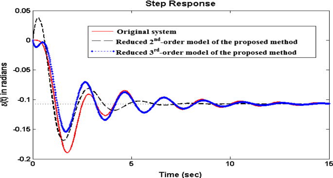

  

  Comparison of $\delta \left( t \right)$ responses for $\Delta V_{\text{ref}} \left( t \right) = 0.05 \;{\text{p}} . {\text{u}} .$ and $\Delta T_{m} \left( t \right) = 0$

  Fig. 8

  

  Comparison of $\delta \left( t \right)$ responses for $\Delta V_{\text{ref}} \left( t \right) = 0$ and $\Delta T_{m} \left( t \right) = 0.05\; {\text{p}} . {\text{u}} .$

  Fig. 9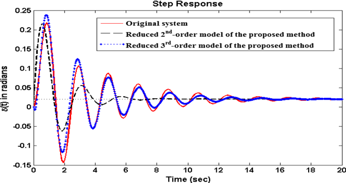

  

  Comparison of $\delta \left( t \right)$ responses for $\Delta V_{\text{ref}} \left( t \right) = 0.05\; {\text{p}} . {\text{u}} .\; {\text{and }}\;\Delta T_{m} \left( t \right) = 0.05 \;{\text{p}} . {\text{u}} .$

  Fig. 10

  

  Comparison of $V_{t} \left( t \right)$ responses for $\Delta V_{\text{ref}} \left( t \right) = 0.05\;{\text{p}} . {\text{u}} .$ and $\Delta T_{m} \left( t \right) = 0$

  Fig. 11

  

  Comparison of $V_{t} \left( t \right)$ responses for $\Delta V_{\text{ref}} \left( t \right) = 0$ and $\Delta T_{m} \left( t \right) = 0.05 \;{\text{p}} . {\text{u}} .$

  Fig. 12

  

  Comparison of $V_{t} \left( t \right)$ responses for $\Delta V_{\text{ref}} \left( t \right) = 0.05\;{\text{p}} . {\text{u}} .\;{\text{and}}\;\Delta T_{m} \left( t \right) = 0.05 \;{\text{p}} . {\text{u}} .$

Table 5 shows that the efficacy of the proposed ROMs is shown by comparing their step ISE and IRE with those of the ROMs obtained from recent and familiar MOR methods in the literature.

Table 5 Comparison of the performance indices ISE and IRE of the ROMs obtained by the proposed method and other existing methods

The step responses in Figs. 7, 8, 9, 10, 11 and 12 indicate that the response of the proposed ROMs seems to be closely matched with the response of the original system. The comparison of performance indices shown in Table 5 shows the dominance of the proposed third-order reduced model over the other ROMs. Moreover, the proposed method produces ROMs with low ISE values along with the satisfactory retention of IRE values. Hence, the proposed method generates ROMs that are very helpful for better understanding the original system, simplifying the control design, reducing computational complexity, making the simulation faster and reducing the memory requirements.

Example 3

The effectiveness of the proposed method can be shown by considering a SMIB system without an automatic excitation control system (AECS). This system gives a sixth-order MIMO uncompensated system with a typical transient response. The transfer function representation of the system based on the numerical values of the state-space matrices $A^{\prime}, B^{\prime}, C^{\prime}\;{\text{and}}\; D^{\prime}$ defined in “Appendix” is given below:

$$ \left[ {G_{6} \left( s \right)} \right] = \left[ {\begin{array}{*{20}c} {g_{11} \left( s \right)} & {g_{12} \left( s \right)} \\ {g_{21} \left( s \right)} & {g_{22} \left( s \right)} \\ \end{array} } \right] = \left[ {\begin{array}{*{20}c} {\frac{{\tilde{\delta }\left( s \right)}}{{\Delta V_{ref} \left( s \right)}}} & {\frac{{\tilde{\delta }\left( s \right)}}{{\Delta T_{m} \left( s \right)}}} \\ {\frac{{\tilde{V}_{t} \left( s \right)}}{{\Delta V_{ref} \left( s \right)}}} & {\frac{{\tilde{V}_{t} \left( s \right)}}{{\Delta T_{m} \left( s \right)}}} \\ \end{array} } \right] = \frac{1}{{D_{6} \left( s \right)}}\left[ {\begin{array}{*{20}c} {a_{11} \left( s \right)} & {a_{12} \left( s \right)} \\ {a_{21} \left( s \right)} & {a_{22} \left( s \right)} \\ \end{array} } \right] $$

(35)

where the common denominator $D_{6} \left( s \right)$ is given by:

$$ \begin{aligned} D_{6} \left( s \right) & = s^{6} + 41.3728s^{5} + 466.3606s^{4} + 1018.1659s^{3} + 6729.8343s^{2} + 4509.30158s + 21414.3562 \\ & \quad {\text{and }} \quad a_{11} \left( s \right) = - 2298.089s - 45961.7802 \\ \end{aligned} $$

$$ a_{12} \left( s \right) = 29.09115s^{4} + 1203.5823s^{3} + 13247.0921s^{2} + 16501.6656s + 54859.6258 $$

$$ a_{21} \left( s \right) = 85.2292s^{3} + 1704.5836s^{2} + 1036.6511s + 20733.0227 $$

$$ a_{22} \left( s \right) = - 1.2596s^{4} - 56.4218s^{3} - 749.4062s^{2} - 2578.6819s - 1642.7642. $$

By applying the proposed method to the above MIMO system with the EDE parameters given in Table 6, the desired ROM transfer function matrix [R_r(s)] is obtained.

Table 6 Parameters used for the EDE algorithm

The general form of the second- and third-order ROMs of MIMO transfer functions is represented by Eqs. (30) and (31). The numerical values of the desired ROM common denominator polynomial coefficients and the corresponding numerator polynomial matrix coefficients obtained from the proposed method are given below.

The numerical values of [R₂(s)] are as follows:

The common denominator polynomial $\tilde{D}_{2} \left( s \right) = s^{2} + 0.356812 s + 5.482879$ and the corresponding numerator polynomial matrix coefficients are

$$ \begin{aligned} c_{11} \left( s \right) & = 6.540557 s - 11.767941 \\ c_{12} \left( s \right) & = 4.384505 s + 14.046123 \\ c_{21} \left( s \right) & = - 2.21327 s + 5.308432 \\ c_{22} \left( s \right) & = - 1.52447 s - 0.420609. \\ \end{aligned} $$

The optimum value of the objective function $\left( I \right) = 3.749298$. The number of generations $\left( g \right)$ taken to attain the optimal second-order reduced model is equal to 80.

Similarly, the numerical values of $\left[ {R_{3} \left( s \right)} \right]$ are as follows:

The common denominator polynomial $\tilde{D}_{3} \left( s \right) = s^{3} + 1.560641s^{2} + 5.320475s + 6.572147$ and the corresponding numerator polynomial matrix coefficients are

$$ \begin{aligned} \bar{c}_{11} \left( s \right) & = 5.99937s^{2} - 13.27889s - 14.105846 \\ \overline{c}_{12} \left( s \right) & = 8.193421s^{2} + 10.073204 + 16.836628 \\ \overline{c}_{21} \left( s \right) & = - 1.07566s^{2} + 4.880326s + 6.363044 \\ \overline{c}_{22} \left( s \right) & = - 1.118678s^{2} - 0.26892s - 0.504171. \\ \end{aligned} $$

The optimum value of the objective function $\left( I \right) = 1.716937$. The number of generations $\left( g \right)$ taken to attain an optimal second-order reduced model is equal to 121.

The effectiveness of the second- and third-order ROMs obtained from the proposed method is shown by comparing their output responses (i.e. $\tilde{\delta }\left( t \right)$ and $\tilde{V}_{t} \left( t \right)$) with the original system responses subjected to the step input changes $\Delta V_{\text{ref}} \left( t \right) = 0.05 \;{\text{p}} . {\text{u}} . \;{\text{and}}\; \Delta T_{m} \left( t \right) = 0.05\; {\text{p}} . {\text{u}} .$ The comparison of the responses is shown in Figs. 13 and 14. The performance of the proposed method is shown by evaluating and comparing ISE and IRE values in Table 7. The efficacy of the proposed method in terms of time domain parameters is shown in Table 8.

Fig. 13

Comparison of $\tilde{\delta }\left( t \right)$ responses for $\Delta V_{\text{ref}} \left( t \right) = 0.05 \;{\text{p}} . {\text{u}} . \;{\text{and}}\;\Delta T_{m} \left( t \right) = 0.05\; {\text{p}} . {\text{u}} .$

Fig. 14

Comparison of $\tilde{V}_{t} \left( t \right)$ responses for $\Delta V_{\text{ref}} \left( t \right) = 0.05 \;{\text{p}} . {\text{u}} .\; {\text{and}}\; \Delta T_{m} \left( t \right) = 0.05\;{\text{p}} . {\text{u}} .$

Table 7 Comparison of the performance indices ISE and IRE of the ROMs obtained by the proposed

Table 8 Comparison of the time domain specifications

From the comparisons made in Tables 7 and 8, we can say that the proposed method generates ROMs with satisfactory retention of the time domain specifications and stability and passivity properties of the original system. Hence, the proposed ROMs effectively help to develop a low-order controller/compensator for controlling the dynamics of the original higher-order system to the desired response value, with a low level of computational effort.

4 Conclusion

In this paper, an effective MOR method for a linear continuous-time system is proposed to obtain a stable and accurate ROM by using the EDE algorithm and IMPPA method. The EDE algorithm is used to determine the denominator polynomial coefficients of the ROM, and the numerator polynomial coefficients are determined by using the IMPPA method. The approach is iterative and progresses with the minimisation of the step ISE between the system and ROM. The proposed method has the inbuilt feature of preserving stability and passivity properties. The ISE values of the proposed ROMs are comparatively lower than those of ROMs obtained by the notable reduction methods available in the literature. The effectiveness of the proposed method has been illustrated by applying it to SISO and MIMO system models. A comparison of the results shows the strength of the proposed method as a new potential approach to MOR. Hence, the ROM obtained by the proposed method validates the analysis, design and development of a lower-order controller for linear higher-order complex systems with less computational effort.

Some new ideas for future work are given here: (1) the proposed research results shall extend to the design of simple and fast controllers for the original higher-order system; (2) this approach shall extend to the reduction of SISO or MIMO continuous-time delay systems, discrete-time systems and controller design; (3) this proposed approach shall extend to the reduction of linear interval systems and controller design.

Appendix

The single-machine infinite-bus (SMIB) power system, which is considered in Example 2, is shown in Fig. 15.

Fig. 15

Single-machine infinite-bus (SMIB) power system

The system under study consists of a three-phase, two-pole 160-MVA turbogenerator with an automatic excitation control system (i.e. a standardised IEEE Type-I exciter with rate feedback and power system stabilising signals) supplying power via a step-up transformer and a high voltage transmission line to an infinite grid. In Fig. 15, $X_{T}$ and $X_{L}$ represent the reactance of the transformer and the transmission line, respectively, and $V_{T}$ and $V_{B}$ are the generator terminal and infinite-bus voltages, respectively.

A detailed block diagram of the SMIB power system [25] is shown in Fig. 16. The numerical values of the parameters that define the total system and its operating point come from [24, 25] and are given below.

Fig. 16

Block diagram representation of the SMIB power system

The nomenclature of the above system parameters is as follows:

$\delta , \omega , V_{T} , P, Q$	$\begin{aligned} {\text{Synchronous}}\;{\text{machine}}\;{\text{torque}}\;{\text{angle}},\;{\text{Speed}},\;{\text{Terminal }}\;{\text{voltage}},\;{\text{Active}}\; {\text{and }} \hfill \\ \;{\text{Reactive}}\;{\text{power}} \hfill \\ \end{aligned}$
$K_{1} , K_{2} , K_{3} , K_{4} ,K_{5} , K_{6}$	${\text{Synchronous machine linear model parameters}}$
$H, T_{a} , T_{e} , T_{m}$	${\text{Synchronous}}\;{\text{machine }}\;{\text{inertia }}\;{\text{constant}},\;{\text{Accelerating}},\;{\text{Electrical}}\;{\text{and}}\;{\text{Mechanical}}\;{\text{torques}}$
$R_{e} , X_{e}$	${\text{Equivalent}}\;{\text{resistance }}\;{\text{and}}\;{\text{Reactance }}\;{\text{of}}\; {\text{external }}\;{\text{system}}$
$E_{q} , E_{FD} , \tau_{d0}$	$\begin{aligned} {\text{Voltage }}\;{\text{proportional}}\; {\text{to}}\; d - {\text{axis}}\;{\text{flux}}\;{\text{linkages}},\;{\text{Field }}\;{\text{voltage}}\;{\text{and}}\;{\text{Open - circuit }} \hfill \\ {\text{time}}\;{\text{constant}} \hfill \\ \end{aligned}$
$K_{E} , S_{E} , \tau_{E}$	${\text{Self-excited}}\;{\text{field }}\;{\text{constant}},\;{\text{Saturation}}\;{\text{function}}\;{\text{and}}\;{\text{Time }}\;{\text{constant}}\;{\text{of}}\;{\text{an}}\;{\text{exciter}}$
$K_{A} , \tau_{A} , V_{R}$	${\text{Regulator }}\;{\text{gain}},\;{\text{Time}}\;{\text{constant}}\;{\text{and}}\;{\text{Output }}\;{\text{voltage}}$
$K_{F} , \tau_{F}$	${\text{Rate }}\;{\text{feedback}}\; {\text{gain}}\; {\text{and}}\; {\text{Time}}\; {\text{constant}}$
$K_{R} , \tau_{R}$	${\text{Transducer }}\;\left( {\text{or}} \right)\;{\text{Filter}}\;{\text{gain}}\;{\text{and}}\;{\text{Time}}\;{\text{constant}}$
$K_{0} ,\tau_{0} , V_{s}$	${\text{Speed}}\;{\text{gain}},\;{\text{Reset }}\;{\text{time-lag}}\;{\text{constant}}\;{\text{and}}\;{\text{Stabiliser}}\;{\text{output}}\;{\text{voltage}}$
$\tau_{1} , \tau_{2} , \tau_{3} , \tau_{4}$	${\text{Lead }}\;{\text{and}}\;{\text{Lag }}\;{\text{time }}\;{\text{constants}}\; \tau \; {\text{of}}\; {\text{the}}\; {\text{power}}\; {\text{system}}\; {\text{stabiliser}}$
$s$	Laplace operator
$\Delta$	Incremental (step) change of input

The numerical values of the system parameters and operating point are as follows:

${\text{Synchronous }}\;{\text{machine}}$	$3{\text{ - phase}}, 160\; {\text{MVA}},\; {\text{power}}\; {\text{factor}} = 0.894,x_{d} = 1.7, x_{q} = 1.6, x_{d}^{\prime} = 0.254 \;{\text{p}} . {\text{u}} . ,$ $\tau_{d0} = 5.9, H = 5.4\; {\text{s}}, \omega_{R} = 314 \;{\raise0.7ex\hbox{${\text{rad}}$} \!\mathord{\left/ {\vphantom {{\text{rad}} {\text{s}}}}\right.\kern-0pt} \!\lower0.7ex\hbox{${\text{s}}$}}$
${\text{Type - I}}\; {\text{exciter}}$	$K_{A} = 50, K_{E} = - 0.17, S_{E} = 0.95, K_{F} = 0.04, K_{R} = 1,K_{0} = 1, \tau_{A} = 0.05,$ $\tau_{E} = 0.95, \tau_{F} = 1.0, \tau_{R} = 0.05, \tau_{0} = 10.0, \tau_{1} = \tau_{3} = 0.44, \tau_{2} = \tau_{4} = 0.092\;{\text{s}}$
${\text{External }}\;{\text{system}}$	$R_{e} = 0.02, X_{e} = 0.4 \;{\text{p}} . {\text{u}} .\left( {{\text{on}}\;160 \;{\text{MVA }}\;{\text{base}}} \right)$
${\text{Operating}} \;{\text{point}}$	$P_{o} = 1.0, Q_{o} = 0.5, E_{\text{FDo}} = 2.5128, E_{qo} = 0.9986, V_{to} = 1.0, T_{mo} = 1.0\;{\text{p}} . {\text{u}} . ,$ $\begin{aligned} \delta_{o} = 1.1966\; {\text{rad}}, K_{1} = 1.133, K_{2} = 1.3295, K_{3} = 0.3072, K_{4} = 1.8235, \hfill \\ K_{5} = - 0.0433, K_{6} = 0.4777. \hfill \\ \end{aligned}$

The system in Fig. 16 can be described in state-space form, as in Eq. (1). The state vector $X\left( t \right)$ is defined with state variables as $X^{\text{T}} \left( t \right) = \left[ {E_{q} \omega \delta v_{1} v_{R} E_{FD} v_{2} v_{3} v_{4} v_{5} } \right]$. The input and output vectors are given by $U^{\text{T}} \left( t \right) = \left[ {\Delta V_{\text{ref}} \Delta T_{m} } \right] \;{\text{and}}\; Y^{\text{T}} \left( t \right) = \left[ {\delta V_{t} } \right]$. For the system parameters and operating points described, the numerical values of the system, input, output and feedforward matrices $A, B, C \;{\text{and}}\; D$, respectively, are given below.

The system, input and output matrices of the SMIB without AECS (i.e. a standard IEEE Type-I exciter without rate feedback (RF) and without power system stabiliser (PSS)) are represented by $A^{\prime}, B^{\prime}\;{\text{and}}\; C^{\prime}$, respectively. The state-space representation of the SMIB system without AECS yields a sixth-order model of the following form:

$$ \left. {\begin{array}{*{20}c} {\frac{{{\text{d}}\tilde{X}\left( t \right)}}{{{\text{d}}t}} = A^{\prime} \cdot \tilde{X}\left( t \right) + B^{\prime} \cdot U\left( t \right)} \\ {Y\left( t \right) = C^{\prime} \cdot \tilde{X}\left( t \right) + D^{\prime} \cdot U\left( t \right)} \\ \end{array} } \right\} . $$

(33)

The state vector $\tilde{X}\left( t \right)$ is defined with state variables as $\tilde{X}^{\text{T}} \left( t \right) = \left[ {\tilde{E}_{q} \tilde{\omega } \tilde{\delta } \tilde{v}_{1} \tilde{v}_{R} \tilde{E}_{\text{FD}} } \right]$.The input and output vectors are given by $U^{\text{T}} \left( t \right) = \left[ {\Delta V_{\text{ref}} \Delta T_{m} } \right]\; {\text{and}}\; Y^{\text{T}} \left( t \right) = \left[ {\tilde{\delta } \tilde{V}_{t} } \right]$, respectively.

References

O.M.K. Alsmadi, S.S. Saraireh, Z.S. Abo-Hammour, A.H. Al-Marzouq, Substructure preservation Sylvester-based model order reduction with application to power systems. Electric Power Compon. Syst. 42(9), 914–926 (2014)
P. Boby, J. Pal, An evolutionary computation-based approach for reduced order modelling of linear systems, in IEEE International Conference on Computational Intelligence and Computing research, @Coimbatore, India, 28–29 Dec (2010). https://doi.org/10.1109/iccic.20
A.K. Choudhary, S. Nagar, Order reduction in z-domain for interval system using an arithmetic operator. Circuits Syst. Signal Process. 38(3), 1023–1038 (2019)
S.R. Desai, R. Prasad, A new approach to order reduction using stability equation and big bang big crunch optimization. Syst. Sci. Control Eng. 1(1), 20–27 (2013)
S.R. Desai, R. Prasad, A novel order diminution of LTI systems using big bang big crunch optimization and routh approximation. Appl. Math. Model. 37(16–17), 8016–8028 (2013)
H.K. Fathy, D. Geoff Rideout, L.S. Louca et al., A review of proper modelling techniques. ASME J. Dyn. Syst. Measur. Control 130(6), 061008-1–061008-10 (2008)
R. Genesio, M. Milanese, A note on the derivation and use of reduced order models. IEEE Trans. Automat. Control 21(1), 118–122 (1976)
D.H. George, R. Luss, Model reduction by minimization of integral square error performance indices. J. Franklin Inst. 327(3), 343–357 (1990)
A. Ghafoor, M. Imran, Passivity preserving frequency weighted model order reduction technique. Circuits Syst. Signal Process. 36(11), 4388–4400 (2017)
W.G. Heffron, R.A. Phillips, Effect of modern amplidyne voltage regulators on the under-excited operation of large turbine generators. AIEE Trans. PAS-71, 692–697 (1952)
M. Imran, A. Abdul Ghafoor, A Frequency limited interval gramians-based model reduction technique with error bounds. Circuits Syst. Signal Process. 34(11), 3505–3519 (2015)
M. Javad, M.G. Karolos, Efficient Modeling and Control of Large-Scale Systems (Springer, Newyork, 2010)
D. Karaboga, S. Okdem, A simple and global optimization algorithm for engineering problems: differential evolution algorithms. Turk. J. Electr. Eng. 12(1), 53–60 (2004)
R.J. Lakshmi, P.M. Rao, C. Chakravarthi, A method for the reduction of MIMO system using interlacing property and coefficient matching. Int. J. Comput. Appl. 1(9), 14–17 (2010)
T.N. Lucas, Optimal model reduction by multipoint pade approximation. J. Franklin Inst. 330(1), 79–93 (1993)
T.N. Lucas, Suboptimal model reduction by multi-point pade approximation. Proc. Inst. Mech. Eng. Part I J. Syst. Control Eng. 208(2), 131–134 (1994)
T.N. Lucas, Constrained suboptimal pade model reduction. Proc. Inst. Mech. Eng. Part I J. Syst. Control Eng. 209(1), 30–35 (1995)
S. Mukherjee, R.C. Mittal, Model order reduction using response-matching technique. J. Frankl. Inst. 342(5), 503–519 (2005)
R. Narayan Panda, P. Sasmita kumara, S. Prasad, S. PrasadaPanigrahi, Reduced complexity dynamic systems using approximate control moments. Circuits Syst. Signal Process. 31(5), 1731–1744 (2012)
A. Narwal, R. Prasad, Order reduction of LTI systems and their qualitative comparison. IETE Tech. Rev. 34(16), 655–663 (2017)
H. Nasirisoloklo, R. Hajmohammadi, M.M. Farsangi, Model order reduction based on moment matching using Legendre wavelet and harmony search algorithm. IJST Trans. Electr. Eng. 39(E1), 39–54 (2015)
K. Nicholas, J.M. McCourt, M. Xia, G. Vijay, On relationships among passivity, positive realness, and dissipativity in linear systems. Automatica 50(4), 1003–1016 (2014)
Y.Y. Nie, X.K. Xie, New criteria for polynomial stability. IMA J. Math. Control Inf. 4(1), 1–12 (1987)
G. Pamar, S. Mukherjee, R. Prasad, Reduced order modelling of linear MIMO systems using genetic algorithm. Int. J. Simul Model 6(3), 173–184 (2007)
D.P. Papadopoulos, Order reduction of linear system models with a time-frequency domain method. J. Franklin Inst. 322(4), 209–220 (1986)
U. Salma, K. Vaisakh, Application and comparative analysis of various classical and soft computing techniques for model reduction of MIMO systems. Intell. Ind. Syst. 1(4), 313–330 (2015)
S. Saxena, Y.V. Hote, Load frequency control in power systems via internal model control scheme and model-order reduction. IEEE Trans. Power Syst. 28(3), 2749–2757 (2013)
A. Sharma, H. Sharma, A. Bhargava, N. Sharma, Power law-based local search in spider monkey optimisation for lower order system modelling. Int. J. Syst. Sci. 48(1), 150–160 (2017)
B. Shivanagouda, V.H. Yogesh, Sahaj Saxena, Reduced-order modelling of linear time invariant systems using big bang big crunch optimization and time moment matching method. Appl. Math. Model. 40(15–16), 7225–7244 (2016)
A. Sikander, R. Prasad, Linear time invariant system reduction using mixed method approach. Appl. Math. Model. 39(16), 4848–4858 (2015)
A. Sikander, R. Prasad, Soft computing approach for model order reduction of linear time-invariant systems. Circuits Syst. Signal Process. 34(11), 3471–3487 (2015)
A. Sikander, P. Thakur, Reduced order modelling of linear time-invariant system using modified cuckoo search algorithm. Soft Comput. Methodol. Appl. 22(10), 3449–3459 (2018)
J. Singh, C.B. Vishwakarma, C. Kalyan, Biased reduction method by combining improved modified pole clustering and improved Pade approximations. Appl. Math. Model. 40(2), 1418–1426 (2016)
J. Singh, C. Kalyan, C.B. Vishwakarma, Two degrees of freedom internal model control-PID design for LFC of power systems via logarithmic approximations. ISA Trans. 72, 185–196 (2018). https://doi.org/10.1016/j.isatra.2017.12.002
R. Stron, P. Kennith, Differential evaluation: a simple and efficient adaptive scheme for global optimization over continuous spaces. J. Glob. Optim. 11(4), 341–359 (1997)
G. Vasu, G. Sandeep, K.V.S. Santosh, Reduction of large scale linear dynamic SISO and MIMO systems using differential evolution algorithm, in IEEE Students Conference on Electrical, Electronics and Computer Science (SCEECS-2012) @ Bhopal, India (2012). https://doi.org/10.1109/sceecs.2012.6184732
G. Vasu, M. Sivakumar, M. Ramalingaraju, A novel model order reduction technique for linear continuous-time system using PSO-DV algorithm. J. Control Autom. Electr. Syst. 28(1), 68–77 (2016)
C.B. Vishwakarma, R. Prasad, MIMO system reduction using modified pole clustering and genetic algorithm. Model. Simul. Eng. (2009). https://doi.org/10.1155/2009/540895
Author information
Authors and Affiliations
Corresponding author
Additional information
Publisher's Note
Springer Nature remains neutral with regard to jurisdictional claims in published maps and institutional affiliations.