Graph Theory

Abstract

We begin by discussing binary relations and functions. Graphs are then introduced, following from binary relations. Some standard graphs are defined, as are connectness and degree. We discuss the Königsberg Bridge problem and traversability. Then general walks are introduced, together with paths and cycles. We then define trees, cycles, and Hamilton circuits, and discuss the Traveling Salesman problem. Finally, we look at graph coloring.

4.1 Relations

4.1.1 First Definitions

A (binary) relation ρ from a set S to a set T is a rule that stipulates, given any element s of S and any element t of T, whether s bears a certain relationship to t (written s ρ t) or not (written $s \,\makebox [0pt][l]{$\backslash $}{\rho}\, t$). For example, if S is the set of living males and T is the set of living females, the relation ρ might be “is the son of”; if s denotes a certain man and t denotes a certain woman, we write s ρ t if s is the son of t, and $s \,\makebox [0pt][l]{$\backslash $}{\rho}\, t$ otherwise.

Binary relations are very common in mathematics. We have already seen relations such as ≤, =, and <, and all of these are relations from ℝ to ℝ (or from ℤ to ℤ, or …). The relation ∣, or “divides,” is a relation from ℤ⁺ to ℤ⁺, or from ℤ⁺ to ℤ. If $\mathcal{P}$ and $\mathcal{Q}$ are any collections of sets, then ⊆ and ⊇ are relations from $\mathcal{P}$ to $\mathcal{Q}$.

Alternatively, we can define a binary relation ρ from the set S to the set T as a set ρ of ordered pairs (s,t), where s belongs to S and t belongs to T, with the notation that s ρ t when (s,t)∈ρ and $s \,\makebox [0pt][l]{$\backslash $}{\rho}\, t$ otherwise. This means that, formally, a binary relation from S to T can be defined as a subset of S×T, the Cartesian product of S and T defined in Section 1.4.

Sample Problem 4.1

Suppose S={1,2,3} and T={1,2,3,4}. Find the sets corresponding to s<t and s ²=t, in the usual arithmetical sense.

Solution

The relation s<t corresponds to the set L, defined by

$$L = \bigl\{(1,2),(1,3),(1,4),(2,3),(2,4),(3,4)\bigr\}.$$

s ²=t has

$$R = \bigl\{(1,1),(2,4)\bigr\}$$

as its the corresponding set.

Your Turn

What are the sets corresponding to s≤t and s≥t?

4.1.2 Relations on a Set

Suppose α is a binary relation from a set A to itself or, in other words, α⊆A×A. Then we say that α is a binary relation on A. One special relation on a set is the identity relation: ι _A is the identity relation on A if a ι _A  b is true precisely when b=a, that is, ι _A ={(a,a):a∈A}. If A is a set of numbers, ι _A is the same as the ordinary relation of equality, =.

There are several important properties that a relation on a set may (or may not) have. Suppose α is a relation on α.

• (i) α is called reflexive if and only if a α a for every a∈A. α is irreflexive if and only if a α a is never true for any element a of A.

• (ii) α is called symmetric if and only if a α b implies b α a or, in other words, if (a,b)∈α implies (b,a)∈α. Since, by the definition of inverse relation, we know that a α b if and only if b α ⁻¹ a, we could say that α is symmetric if and only if α=α ⁻¹. α is called antisymmetric if and only if a α b and b α a together imply a=b or, in other words, α∩α ⁻¹⊆ι _A . If a α b and b α a can never both be true, then α is called asymmetric, or sometimes skew. (If a α b and b α a are never both true, then the truth of (a α b∧b α a) implies that a α a is vacuously true, so all asymmetric relations are antisymmetric, but this gives us no information.)

• (iii) α is called transitive if and only if a α b and b α c together imply a α c, and atransitive if and only if, whenever a α b and b α c, $a \,\makebox [0pt][l]{$\backslash $}{\alpha}\,c$, or in other words, if and only if α∩αα=∅.

In particular, a relation is called an equivalence relation if it is reflexive, symmetric, and transitive.

Sample Problem 4.2

What are the reflexive, symmetric, and transitive properties of < and ≤ on the set ℤ? Is either relation an equivalence relation?

Solution

< is irreflexive (a<a is never true) while ≥ is reflexive (a≤a is always true). Both relations are antisymmetric, but < is in fact asymmetric. Both are transitive. Neither is an equivalence relation.

Your Turn

What are the reflexive, symmetric and transitive properties of = and ≥ on ℤ? Is either relation an equivalence relation?

The relation of adjacency on the set of integers, defined by i α j if and only if |i−j|=1 for i and j positive integers, is irreflexive (since |i−i|=0), symmetric (since |i−j|=|j−i|) and not transitive (since 1 α 2 and 2 α 3 but $1\,\makebox [0pt][l]{$\backslash $}{\alpha}\, 3$). It is in fact atransitive, for i α j and j α k together imply i=j±1 and k=j±1, so i=k or i=k±2, but i cannot equal c±1. So $a\,\makebox [0pt][l]{$\backslash $}{\alpha}\, c$.

The properties of relations can be exhibited even in quite small cases. For example, say A={1,2,3} and consider the relation β on A, defined by

$$\beta= \bigl\{(1,1),(2,2)\bigr\}.$$

Since $\iota_{A} \not\subseteq\beta$, it is not reflexive, but since ι _A ∩β≠∅, it is not irreflexive either. Since β=β ⁻¹, it is symmetric, and since β∩β ⁻¹⊆ιA, it is also antisymmetric. Since ββ=β, it is transitive.

4.1.3 Functions

A function, or mapping, f from a set S to a set T, is a rule that associates with each member of S exactly one member of T. In other words, a function is a special kind of relation from S to T, one in which each element of S occurs as the first element of precisely one ordered pair. This uniqueness property is the main point of the idea of a function.

The set S is called the domain of the function, and the set T its codomain. If we used notation consistent with that of the last section, we would write f⊆S×T, but more often when dealing with functions we write f:S→T; the set form is then called the defining set or associated set of f. To indicate the correspondence between elements, we could again write (s,t)∈f, but more often we write f(s)=t, as, for example, in familiar algebraic functions like f(x)=x ³−3x+1.

The image of x under f is the value f(x); if R is any subset of S, then f(R)={f(r):r∈R} is the set of images of elements of R and is called the image of R. In particular f(S), the image of S, is called the range of f and necessarily f(S)⊆T. To avoid trivial cases, it is usual to require that the domain of f should not be empty.

The composition of two functions is defined just as the composition of relations is. In functions, composition is defined as “first perform one function, then the other” (where performing f means replacing the value x by f(x)). The composition “first f, then g” is written g(f(x)), and this can be interpreted as defining a new function g(f), by the rule

$$g(f) (x) = g\bigl(f(x)\bigr).$$

In order for g(f)(x) to be defined, it is necessary that every value of f(x) be in the domain of g. This will not necessarily be true for all x in $\mathcal{D}(f)$; in fact, the domain of g(f) is the set of all elements x in the domain of f such that f(x) is in the domain of g.

This method of combining functions is not commutative; quite possibly g(f) and f(g) will be different functions. In fact, one might be defined and the other not. However, composition is associative.

Sample Problem 4.3

S is the set of all real numbers other than 0 and 1. Consider the following functions from S to S:

Find formulae for f ₂(f ₂), f ₃(f ₅), and f ₅(f ₃), and verify that they are all members of the original set of six functions. Use these to verify that composition is not commutative.

Solution

So f ₂(f ₂)=f ₁, f ₃(f ₅)=f ₄, and f ₅(f ₃)=f ₆.

Observe that f ₅(f ₃)≠f ₃(f ₅), an example of non-commutativity.

Your Turn

Find formulae for f ₁(f ₁), f ₂(f ₄), and f ₅(f ₆), and verify that they are all members of the original set of six functions.

4.1.4 One-to-One and Onto Functions

Two properties of functions are particularly important: we say that a function f is one-to-one if f(s ₁)=f(s ₂) always implies s ₁=s ₂ for any $s_{1},s_{2} \in \mathcal{D}(f)$; we say that f is onto if f(S)=T or, in other words, if for every t∈T, there exists an s∈S such that f(s)=t.

These properties depend on the domain of f. For example, consider the function f defined by f(x)=x ² or f={(x,x ²):x∈ℝ}, which associates its square with each real number. This satisfies the definition of function, for if we choose x, then x ² is uniquely determined.

• (i) If we define the domain of f to be the set ℝ of all real numbers, and the codomain to be ℝ also, then f is neither one-to-one (since f(x)=f(−x)) nor onto (since f(ℝ)={y∈ℝ:y≥0}).

• (ii) If instead we define the domain of f to be the set of all non-negative real numbers, but let the codomain still be the whole of ℝ, then f is one-to-one but is not onto.

• (iii) If we let the domain of f be ℝ but restrict the codomain to be the set of all non-negative real numbers, then f is onto, but is not one-to-one.

• (iv) If both the domain and the codomain are defined to be the set of non-negative reals, then f is both one-to-one and onto.

4.1.5 Inverse Functions

Given any set S, we can define the identity function ι _S :S→S by ι _S (s)=s for every s∈S; in other words,

$$\iota_S = \bigl\{(s,s) : s \in S\bigr\}.$$

For a function, as for any relation, we can define an inverse relation. If the function is, say f(x)=x ², and if we let the domain and the codomain equal ℝ, then the inverse relation f ⁻¹ contains the pairs (4,2) and (4,−2), so it is not a function: f ⁻¹(x) would not be uniquely defined. This raises an important question: when is the inverse relation of a function also a function? The following theorem gives the necessary and sufficient conditions. You may omit the proof on a first reading.

Theorem 9

Let f be a function, f:S→T. Then the inverse relation f ⁻¹ of f is a function from T to S if and only if f is one-to-one and onto.

Proof

(i) Suppose f is one-to-one and onto. Since f is one-to-one, each element of T occurs as the second element of at most one ordered pair in f; since f is onto, each element of T occurs as the second element of at least one ordered pair in f. Hence if t∈T, exactly one ordered pair (s,t)∈f.

Now consider the inverse relation: (t,s)∈f ⁻¹ exactly when (s,t)∈f. Hence for every t∈T, exactly one ordered pair (t,s)∈f ⁻¹, so f ⁻¹ is a function from T to S.

(ii) Suppose conversely that f ⁻¹ is a function from T to S. Then for every t∈T, exactly one ordered pair (t,s)∈f ⁻¹ and hence exactly one ordered pair (s,t)∈f. Since at least one ordered pair has t as its second element for each t∈T, we see that f is onto; since at most one ordered pair has t as its second element for each t∈T, we see that f is one-to-one.  □

Notice that the function f ₁ in Sample Problem 4.3 is the identity function on the set S, and in that problem we showed that f ₂ is its own inverse.

Sample Problem 4.4

What is the inverse of the function f ₄ from Sample Problem 4.3?

Solution

f ₄(x)=1/(1−x). Say y=1/(1−x). Then 1−x=1/y so x=1−1/y=(y−1)/y. So $f_{4}^{-1}(y) =(y-1)/y$. So $f_{4}^{-1} = f_{6}$.

Your Turn

What is the inverse of the function f ₃ from Sample Problem 4.3?

Exercises 4.1 A

• 1. Suppose S={1,2,3,4,5,6,7,8,9}. In each part, a binary relation from S to itself is defined. For each of these relations, what is the corresponding subset of S×S?

  • (i) x α y means x=y ².

  • (ii) x β y means x divides y.

  • (iii) x γ y means x ²+y=12.

• 2. Relations α and β are binary relations from S={1,2,3} to T={1,2,3,4} defined by

  • x α y means x=y ²;

  • x β y means x=y−1.

  For each of these relations, what is the corresponding subset of S×T?

• 3. The relations α, β and γ on the set {1,2,3} are defined by the sets

  

  Which of these relations are:

  • (i) Reflexive;

  • (ii) Irreflexive;

  • (iii) Symmetric;

  • (iv) Antisymmetric;

  • (v) Asymmetric;

  • (vi) Transitive?

• 4. The following are relations from the set ℤ⁺ of positive integers to itself. Determine whether each relation has each of the following properties: reflexivity, symmetry, antisymmetry, transitivity:

  • (i) m+n≥50;

  • (ii) m+n is odd;

  • (iii) mn is odd;

  • (iv) m ²−n ² is even.

• 5. Which, if any, of the relations in Exercises 3 and 4 are equivalence relations?

• 6. Suppose S={1,2,3,4}. Is the given set a function from S to S?

  • (i) {(1,4),(2,3),(3,2),(2,1),(4,4)};

  • (ii) {(2,1),(3,4),(1,4),(2,1),(4,2)};

  • (iii) {(1,4),(2,1),(3,4),(4,1),(3,4)};

  • (iv) {(1,2),(2,2),(3,1),(4,2)}.

• 7. Find the inverses of the following functions.

  • (i) f ₆:S→S from Sample Problem 4.3, where S is the set of all real numbers other than 0 and 1.

  • (ii) f:ℝ→ℝ⁺, where ℝ is the set of real numbers, ℝ⁺ is the set of positive real numbers and

    $$f(x) = \left \{ \begin{array}{l@{\quad}l}2-x & \mbox{if } x \le1, \\1/x & \mbox{if } x > 1.\end{array} \right .$$

• 8. In each case, is the function one-to-one? Is it onto?

  • (i) f:K→K where K={1,2,…,k} and f(1)=k, f(j)=j−1 when j=2,3,…,k.

  • (ii) f:ℤ⁺→{0,1,2,3}, where ℤ⁺ is the set of positive integers, and

    $$f(j) = \left \{ \begin{array}{l@{\quad}l}0 &\mbox{if } 7 \makebox[0pt][l]{$\, \backslash$}\mid j, 3 \mid j, \\1 &\mbox{if } 7 \mid j, 3 \makebox[0pt][l]{$\, \backslash$}\mid j, \\2 &\mbox{if } 21 \mid j, \\3 &\mbox{otherwise. }\end{array} \right .$$

  • (iii) f:ℝ→ℝ⁺, where f(y)=y ².

Exercises 4.1 B

• 1. Suppose S={1,2,3,4,5,6,7,8,9}. In each part, a binary relation from S to itself is defined. For each of these relations, what is the corresponding subset of S×S?

  • (i) x α y means x+y=9.

  • (ii) x β y means 2x<y.

  • (iii) x γ y means x−y=0.

  • (iv) x δ y means x−y>5.

  • (v) x ε y means 2x=3y.

  • (vi) x ξ y means x ²<y−3?

  • (vii) x η y means x ²>y+6.

• 2. Relations α and β are binary relations from S={1,2} to T={1,2,3} defined by

  • x α y means y=x ²−1;

  • x β y means xy>y.

  For each of these relations, what is the corresponding subset of S×T?

• 3. Relations α and β are binary relations from S={1,2,3} to T={1,2,3,4} defined by

  • x α y means y=x ²;

  • x β y means x=y+1.

  For each of these relations, what is the corresponding subset of S×T?

• 4. A group of people, denoted by A,B,…, are at a party. Consider the following relations: is each reflexive, symmetric, antisymmetric, asymmetric or transitive?

  • (i) A α B means A and B spoke to each other at the party.

  • (ii) A β B means A spoke to B at the party.

  • (iii) A γ B means A and B come from the same city.

  • (iv) A δ B means A and B met for the first time at the party.

  • (v) A ε B means A is the father of B.

• 5. The following are relations from the set ℤ⁺ of positive integers to itself. Determine whether each relation has each of the following properties: reflexivity, symmetry, antisymmetry, transitivity.

  • (i) m is divisible by n.

  • (ii) m+n is even.

  • (iii) mn is even.

  • (iv) 3∣(m+n).

  • (v) mn>m+n.

• 6. Is the given relation α an equivalence relation on the given set S?

  • (i) $S = \mathcal{R}$, a α b means ab≥0.

  • (ii) $S = \mathcal{R}$, a α b means ab>0.

  • (iii) S is the set of all non-zero real numbers, a α b means ab>0.

  • (iv) S=ℤ⁺, a α b means a and b have greatest common divisor 16.

• 7. Which, if any, of the relations in Exercises 5 and 4 are equivalence relations?

• 8. The relation  α  from the set ℤ⁺ of positive integers to itself is defined by

  $$r \,{\alpha}\, s \mbox{ means } rs \mbox{ is a perfect square.}$$

  Prove that  α  is an equivalence relation.

• 9. Suppose S={1,2,3,4}. Is the given set a function from S to S?

  • (i) {(1,1),(3,1),(4,3)};

  • (ii) {(1,4),(2,4),(3,3),(4,2)};

  • (iii) {(1,1),(3,1),(1,2),(4,2)};

  • (iv) {(2,2),(1,2),(2,1),(3,4),(4,2)};

  • (v) {(1,1),(2,1),(3,1),(4,3)};

  • (vi) {(1,1),(2,1),(4,1)};

  • (vii) {(1,4),(2,1),(3,3),(4,2)};

  • (viii) {(1,1),(3,1),(1,2),(4,2),(1,2)};

  • (ix) {(2,2),(1,2),(2,1),(1,1)}.

• 10. In each case, is the function one-to-one? Is it onto?

  • (i) f:K→K where K={1,2,…,k} and f(j)=j+1, for j=1,2,…,k−1,f(k)=1.

  • (ii) f:ℚ→ℚ, where f(q)=q ³ for q∈ℚ. (ℚ denotes the set of rational numbers.)

  • (iii) f:ℝ⁺→ℝ⁺ where $f(x) = \sqrt{x}$.

  • (iv) f:ℝ→ℝ^∗, where f(y)=y ²+1.

• 11. Find the inverses of the following functions.

  • (i) f ₅:S→S from Sample Problem 4.3, where S is the set of all real numbers other than 0 and 1.

  • (ii) f ₃:S→S from Sample Problem 4.3, where S is the set of all real numbers other than 0 and 1.

  • (iii) g:ℝ→ℝ, where ℝ is the set of real numbers and

    $$g(x) = \left \{ \begin{array}{l@{\quad}l}2x & \mbox{if } x < 0, \\3x & \mbox{if } x \ge0.\end{array} \right .$$

  • (iv) g:ℝ→ℝ, where ℝ is the set of real numbers and

    $$g(x) = \left \{ \begin{array}{l@{\quad}l}x & \mbox{if } x < 0, \\2\sqrt{x} & \mbox{if } 0 \le x < 1, \\x+1 & \mbox{if } x \ge1.\end{array} \right .$$

4.2 Graphs

4.2.1 Graphs and Multigraphs

Suppose we want to describe the roads joining various towns in order to plan an itinerary. If our only desire is to list the towns that will be visited, in order, we do not need to know the physical properties of the region, such as hills, whether different roads cross, or whether there are overpasses. The important information is whether or not there is a road joining a given pair of towns. In these cases, we could use a complete road map, with the exact shapes of the roads and various other details shown, but it would be less confusing to make a diagram as shown in Figure 4.1(a), that indicates roads joining B to C, A to each of B and C, and C to D, with no direct roads joining A to D or B to D.

Fig. 4.1

Representing a road system

In some cases, there is a choice of routes between two towns. This information may be important: you might prefer the freeway, which is faster, or you might prefer the more scenic coast road. In this case, the diagram does not contain enough information. For example, if there had been two different ways to travel from B to C, this information could be represented as in the diagram of Figure 4.1(b).

Sample Problem 4.5

Suppose the road system connecting towns A, B, and C consists of two roads from A to B, one road from B to C, and a bypass road directly from A to C. Represent this road system in a diagram.

Solution

Your Turn

Draw a diagram to represent the road system connecting towns A, B, C, D, with one road from A to B, one from A to C, two from A to D, and one from B to C.

The sort of diagram shown in Figure 4.1(a) is called a linear graph, or usually simply called a graph. The dots representing towns are called vertices, while the lines representing the road links are called edges.

We make a formal definition, and set up some notation, as follows: a graph G consists of a finite set V or V(G) of objects called vertices, together with a set E(G) of pairs of vertices that are called edges. The two vertices belonging to an edge are called its endpoints; we say they are adjacent, and say the edge joins them.

In the diagram representing a graph, an edge {x,y} is shown as a line from x to y. This is usually drawn as a straight line segment, but not always; the only important thing is that it joins the correct points. Moreover, the position of the points is not fixed. For these two reasons, one graph can give rise to several drawings that look quite dissimilar. For example, the three diagrams in Figure 4.2 all represent the same graph. Although the two diagonal lines cross in the first picture, their point of intersection does not represent a vertex of the graph.

Fig. 4.2

Three representations of the same graph

The definition of a graph does not allow for two edges with the same endpoints. Either a pair of vertices is an edge or it is not. However, there are some situations where we wish to represent several different links between two vertices. The road system modeled in Figure 4.1(b) is an example. The lines representing the two roads from B to C in that figure will be called multiple edges. We say there is a multiple edge of multiplicity 2 joining B to C. The diagram is called a multigraph. In order to emphasize the fact that multiple edges are not allowed in graphs, the term simple graph is sometimes used.

4.2.2 Digraphs

Some road systems contain one-way roads. These can be modeled by assigning a direction to some or all of the edges. Such a model is called a directed graph, or digraph.

Formally, we define a digraph to be a finite set v of objects called vertices together with a finite set of directed edges, or arcs, which are ordered pairs of vertices. So a digraph is like a graph except that each edge is allocated a direction—one vertex is designated a start and the other is a finish. It is important to observe that, unlike a graph, a digraph can have two arcs with the same endpoints, provided they are directed in opposite ways. If multiple arcs can occur, the object would be called a directed multigraph.

Sample Problem 4.6

A road system connecting towns A, B, C, and D consists of two roads joining A and B, one road from B to C, one road from C to D, and one-way roads from A to C and from C to A. Represent this road system in a diagram.

Solution

Your Turn

A road system connecting towns A, B, C, and D consists of one road joining A and B, a one-way road from B to C, a one-way road from C to D, and a one-way road from D to B. Represent this road system in a diagram.

The idea of adjacency needs further consideration in digraphs. Associated with a vertex x are the two sets

(A(x) consists of the vertices after x, and B(x) means before x.) A vertex x is called a source in the digraph if B(x) is empty and a sink if A(x) is empty.

Sample Problem 4.7

Describe the adjacencies in the graph

Solution

$$\begin{array}{rcl@{\qquad}rcl}A(a) & = & \{ b,c\} , & B(a) & = & \emptyset,\\A(b) & = & \emptyset, & B(b) & = & \{ a,c,d \} ,\\A(c) & = & \{b,d\} , & B(c) & = & \{ a\} , \\A(d) & = &\{ b\} , & B(d) & = & \{ c\} ;\end{array}$$

a is a source and b is a sink.

4.2.3 Graphs and Binary Relations

Suppose G is a graph with vertex set V(G). The binary relation ∼, where x∼y means x is adjacent to y, is a symmetric, antireflexive binary relation on V(G).

On the other hand, any binary relation can be represented by a diagram. If the relation is symmetric and antireflexive, the diagram will be a graph. If the binary relation is not symmetric, the lines on the diagram will be directed, and if there are no loops, the diagram is a digraph. So the study of (simple) graphs and digraphs is exactly the same as the study of antireflexive binary relations.

The phrase “looped graph” can be used to describe the diagram of a symmetric relation ∼ in which x∼x is sometimes true, but be careful: a “looped graph” is not really a graph! Similarly, we can discuss looped digraphs. The phrase “infinite graph” means an object defined like a graph, in which the vertex-set can be infinite, and these are useful in discussing binary relations on infinite sets.

4.2.4 Graphical Models

So far we have concentrated on graphs as models of roads or pathways. Graphs and digraphs can be used to model many real-life situations. We shall now describe several examples of graphical models.

In many cases, a weight is associated with each edge or with each vertex. This is a real number, usually positive or non-negative, that measures some attribute of the thing being represented. Typical weights include costs, durations, and capacities.

Telephone Networks

Graphs can be used to model telephone systems in several ways. For example, each user might be denoted by a vertex. Two vertices are joined by an edge when the corresponding users can communicate by a local call. In another graph, the vertices could represent local areas. An edge means that a long distance call can be routed directly between two areas. The routing used to make longer connections correspond to sequences of edges.

Electric Circuits

An electric circuit can be viewed as a number of special places, which we shall call nodes, joined by wires. At any time a wire either carries a current or does not. A node means any point at which something more can happen than simply a current being carried. For example, a node might be an alarm (which will sound when certain wires connected to it carry a current), a light bulb, a point where current can be input to the system or one where current can flow out to a device or another circuit, or a switch. Nodes are represented by vertices and wires by edges. A computer network is a special example of an electric circuit, with vertices representing the computers and edges representing connections by which computers can communicate.

Deliveries

A delivery company might operate as follows. Every day trucks travel on a regular schedule, between some of their depots but not others. Perhaps they travel between St. Louis and Chicago, and between Chicago and Detroit, but there is no service between St. Louis and Detroit. Goods sent from St. Louis to Detroit must be sent to Chicago one day, and on to Detroit the next day. This transportation network can be represented as a graph whose vertices are the depots and whose edges are the routes.

One natural weight on this graph is the capacity. If three trucks travel from Chicago to Detroit each day, and each can carry 10000 pounds of freight, then that edge would be assigned weight 30000. Another weight is the price charged per pound to transport goods. Yet another is the cost of running each truck.

Commodity Flow

Suppose a company manufactures refrigerators in three factories and sells them from five wholesale stores. The movement of computers to retailer can be represented by a directed graph like

where a ₁, a ₂, a ₃ represent the factories and b ₁, b ₂, b ₃, b ₄, b ₅ represent the wholesale stores.

In this case, there are two obvious weights, the capacity of an edge (the number of truckloads that can be delivered from the particular factory to the particular wholesaler per day) and the cost of sending refrigerators. The usual problems are to ensure that each wholesaler receives as many refrigerators as needed, while no factory exceeds capacity. In other words, can supply meet demand? If this is possible, we are interested to know the cheapest way of satisfying these conditions. Often it will be possible to ship refrigerators between wholesalers. In that case, the model will contain edges joining some of the b _i , but of course using them will entail an extra cost.

Tournament Schedules

Suppose several baseball teams play against each other in a league. The competition can be represented by a graph with the teams as vertices and with an edge xy representing a game between teams x and y. Such a league, where two participants meet in each game, is called a tournament. Sometimes multiple edges will be necessary; sometimes two teams do not meet. The particular case where every pair of teams plays exactly once is called a round robin tournament.

In a round robin tournament, the result of each game can be shown in a directed graph, where the edge is directed from the winning team to the loser. The digraph that results from this representation is rather special: if x and y are any two vertices, then exactly one of the two possible arcs (x,y) and (y,x) occurs in the digraph. The word “tournament” is also used for directed graphs with this property.

Exercises 4.2 A

• 1. Draw diagrams to represent the following road systems.

  • (i) There are three towns, A, B, and C. There are two roads from A to B, two roads from B to C, and a bypass road from A to C.

  • (ii) There are four towns, A, B, C, and D. There are two roads from A to B, two roads from B to C, two roads from C to D, and one road from A to D.

• 2. For each of the following digraphs, list all the arcs and list the members of A(x) and B(x) for each vertex x.

  

• 3. Draw a diagram for each binary relation defined in Exercise 4.1A.1. Which if any are graphs? Which if any are digraphs?

• 4. Draw a diagram for each binary relation defined in Exercise 4.1A.2. Which if any are graphs? Which if any are digraphs?

Exercises 4.2 B

• 1. For each of the following digraphs, list all the arcs and list the members of A(x) and B(x) for each vertex x.

  

• 2. In each case, draw a diagram to represent the road system.

  • (i) There are four towns, A, B, C, and D. There are two roads from A to B, one road from B to C, two roads from B to D, and one road from C to D.

  • (ii) There are four towns, A, B, C, and D. There is one road joining each of the following pairs: A and B, A and C, A and D, B and D, C and D.

  • (iii) There are four towns, A, B, C, and D. There is one road from A to B, two roads from B to C, two roads from C to D, and one road from B to D.

• 3. Draw a diagram for each binary relation defined in Exercise 4.1B.1. Which if any are graphs? Which if any are digraphs?

• 4. Draw a diagram for each binary relation defined in Exercise 4.1B.3. Which if any are graphs? Which if any are digraphs?

• 5. Draw a digraph to represent a tournament between teams V,W,X,Y,Z after the following matches. V beat W, V beat X, W beat X, Y beat V, Y beat Z, Z beat X. If it is a round robin tournament, how many matches remain to be played?

4.3 Some Properties of Graphs

4.3.1 Degree

We define the degree or valency d(x) of the vertex x to be the number of edges that have x as an endpoint.

Sample Problem 4.8

What are the degrees of the vertices in the following graph?

Solution

There are three vertices of degree 4 (the upper vertices in the figure), while the other four have degree 3.

Your Turn

What are the degrees of the vertices on the following graphs?

Sample Problem 4.9

Can you find a graph on six vertices whose vertices have degrees 5, 3, 2, 2, 1, 1?

Solution

Suppose such a graph exists. The vertex of degree 5 must lie on five edges, and their endpoints must all be different. (The problem asks for a graph, not a multigraph, so there are no multiple edges.) As there are six vertices, the vertex of degree 5 is adjacent to all the other vertices. We know the graph must contain the following configuration:

Moreover, the black vertices lie on no further edges. It is now necessary to add edges, touching the clear vertices only, so that two edges touch one vertex and one edge touches each of the other vertices, in order to make their degrees 3, 2, 2. This is easily done, as follows:

Your Turn

Can you find a graph on six vertices whose vertices have degrees 5, 4, 2, 1, 1, 1?

Theorem 10

In any graph or multigraph, the sum of the degrees of the vertices equals twice the number of edges (and consequently the sum of the degrees is an even integer).

Proof

Suppose the graph or multigraph has e edges; label the edges, say y ₁,y ₂,…,y _e . Consider a list in which each edge appears twice, once for each endpoint. For example, if y ₁ has endpoints x ₄ and x ₇, you might make entries y ₁:x ₄ and y ₁:x ₇. Vertex x will appear in precisely d(x) entries, so the total number of entries equals the sum of the degrees of the vertices. On the other hand, each edge appears twice, so the total number of entries equals twice the number of edges.  □

We shall call a vertex odd if its degree is odd, and even if the degree is even.

Corollary 1

In any graph or multigraph, the number of odd vertices is even.

4.3.2 Some Standard Graphs

Given a set S of v vertices, the graph formed by joining each pair of vertices in S is called the complete graph on S and denoted K _S . We write K _v to mean any complete graph with v vertices. The three drawings in Figure 4.2 are all representations of K ₄. On the other hand, a graph with no edges—consisting of v isolated vertices—will be called empty, and denoted $\overline{K}_{v}$.

Further standard graphs are the complete bipartite graphs. If S and T are two disjoint sets of vertices, the complete bipartite graph based on S and T has vertex set S∪T, consisting of all elements of S and all elements of T, and its edges are all the pairs with one vertex in S and the other in T. There are no edges joining members of the same set. We write K _m,n for any complete bipartite graph in which one vertex set has m vertices and the other has n. The graph in Sample Problem 4.8 is a copy of K _4,3.

If G is a graph, it is possible to choose some of the vertices and some of the edges of G in such a way that these vertices and edges again form a graph, say H. H is then called a subgraph of G; we write H≤G. A subgraph of a complete bipartite graph is simply called a bipartite graph.

Sample Problem 4.10

Suppose a plant contains m machines, and there are n workers who can operate them. Each worker is qualified to use some of the machines. Model this situation with a graph.

Solution

We represent the machines by a set of vertices S and the workers by a set of vertices T. The vertex-set is S∪T. There is an edge from (machine) x to (worker) y if y is qualified to use x. The graph will be bipartite, a subgraph of the graph K _m,n with vertex sets S and T.

4.3.3 Walks and Connectedness

We define a walk in a graph G to be any finite sequence of vertices x ₀,x ₁,…,x _n and edges y ₁,y ₂,…,y _n of G:

$$x_0,y_1,x_1,y_2,\ldots,y_n,x_n,$$

where the endpoints of y _i are x _i−1 and x _i for each i. The length of a walk is its number of edges. The walk written above might be called an x ₀ x _n -walk of length n. A closed walk, or circuit, is one in which the first and last vertices are the same.

Walks are called simple if there is no repeated edge. A walk in which no vertex is repeated is a path.

There is no such thing as a closed path—the last vertex is a repeat of the first—but we shall define a cycle to be a closed simple walk with no vertex repeats except for the endpoints.

We say two vertices are connected when there is a walk joining them. A graph is called connected if every pair of its vertices are connected. If a graph is not connected, it falls into two or more parts with no edges joining them. The connected parts of a graph are called components. So two vertices of G are connected if and only if they lie in the same component of G.

Among connected graphs, some are connected so slightly that removal of a single vertex or edge will disconnect them. Such vertices and edges are quite important. A vertex x is called a cutpoint in G if G−x contains more components than does G; in particular if G is connected, then a cutpoint is a vertex x such that G−x is disconnected. Similarly, a bridge is an edge whose deletion increases the number of components.

Sample Problem 4.11

If a graph represents a road network, what is the interpretation of a bridge? Why are such edges important?

Solution

A bridge represents a road whose deletion would cut people in part of the network off from those in another part. (Often a real bridge, over a river, etc., plays this role.) It is important to recognize such roads so that extra effort can be taken to keep them open to traffic. For example, the highways department might give special priority to keeping them plowed in winter.

Your Turn

In such a graph, what is the interpretation of a cutpoint?

4.3.4 Distance

If vertices x and y are adjacent, then there is a path of length 1 from x to y, and we shall say that the distance from x to y is 1. If x and y are connected, there may be several paths joining them, and we define the distance between them to be the length of the shortest path joining them; we denote it D(x,y). For completeness, we define D(x,x) to be 0.

Sample Problem 4.12

Find the distance between every pair of vertices in the graph (a) below.

Solution

There are two different kinds of vertex in the graph. In each part of the following figure, one vertex is highlighted and the number against a vertex shows the distance from the highlighted one.

Your Turn

Find the distance between every pair of vertices in graph (b).

Distance arises in the example of a communications network. The vertices of a graph might represent computers. If two computers are directly linked, the corresponding vertices are adjacent so that edges represent direct links. Often messages from one computer to another are sent by way of another machine—e-mail messages are often relayed through several intermediate computers. Two computers can communicate if the corresponding vertices are connected.

The physical separation between the computers is irrelevant. The number of times the signal is relayed may well be significant: the more relays, the greater the chance of a delay. (Direct communication between computers, by media such as telephone cables, is practically instantaneous, but delays may occur when an intermediate link is busy or down.) So the distance between vertices is a measure of the possibility of delay.

In this example, we are often interested in the worst case—what is the worst delay that can occur? To measure this, we define the eccentricity ε(x) of vertex x in a connected graph to be the largest value of D(x,y), where y ranges through all the vertices. The diameter D=D(G) of G is the maximum value of ε(x) for all vertices x of G, while the radius R=R(G) is the smallest value of ε(x).

Sample Problem 4.13

Find the diameter and radius of graph (a) of Sample Problem 4.12.

Solution

Four vertices have eccentricity 4, and the others have eccentricity 3. So D=4, R=3.

Your Turn

Find the diameter and radius of the graph (b) of Sample Problem 4.12.

Theorem 11

In any graph G,

$$R(G) \le D(G) \le2R(G).$$

Proof

Clearly, D(G) equals the maximum distance between any two vertices in G. Say x and y attain this maximum distance, so that D(x,y)=D(G), and say z is a vertex for which ε(z)=R(G). As R is a distance between two vertices, necessarily R≤D. But by definition D(z,t)≤ε(z)=R(G) for every vertex t, so D(G)=D(x,y)≤D(x,z)+D(z,y)≤2R(G).  □

Exercises 4.3 A

• 1. What are the degrees of the vertices in the following graphs?

  

• 2. Draw the graphs K ₅ and K ₆. What are the degrees of the vertices in these graphs?

• 3. Can you find a connected graph with four vertices whose degrees are 2, 2, 1, 1?

• 4. Is there a connected graph with four vertices whose degrees are 3, 3, 1, 1?

• 5. The n-wheel W _n has n+1 vertices {x ₀,x ₁,…,x _n }; x ₀ is joined to every other vertex and the other edges are

  $$x_1x_2,x_2x_3,\ldots,x_{n-1}x_n, x_nx_1.$$

  How many edges does W _n have? What are the degrees of its vertices?

• 6. Identify all cutpoints and bridges in the graphs of Exercise 1.

• 7. How many edges are there in K ₇?

• 8. How many edges are there in K _n ?

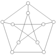
• 9. What are the diameter and radius of the following graph, which is called the Petersen graph?

  

• 10. Find all paths from s to t in the following graph.

  

  What is the length of each path? What is the distance from s to t?

• 11. Find all paths from s to t in the following graph.

  

  What is the length of each path? What is the distance from s to t?

Exercises 4.3 B

• 1. Draw the graphs K _2,5, K _3,3, K ₇, and K _3,4. What are the degrees of the vertices in these graphs?

• 2. Can you find graphs whose vertices have the following sets of degrees?

  • (i) 3, 2, 2, 1;

  • (ii) 5, 3, 3, 1;

  • (iii) 5, 3, 3, 2, 2;

  • (iv) 4, 4, 3, 3, 2;

  • (v) 5, 3, 3, 3, 1, 1;

  • (vi) 3, 3, 3, 3, 2, 2;

  • (vii) 2, 2, 2, 1;

  • (viii) 3, 3, 3, 1, 1, 1;

  • (ix) 4, 3, 3, 2, 2;

  • (x) 4, 4, 2, 2, 2, 1, 1;

  • (xi) 5, 4, 3, 3, 2, 1;

  • (xii) 3, 3, 3, 3, 3, 2, 2.

• 3. What are the degrees of the vertices in the following graphs?

  

  Identify all cutpoints and bridges in these graphs.

• 4. What are the degrees of the vertices in the following graphs?

  

  Identify all cutpoints and bridges in these graphs.

• 5. The n-star K _1,n has n+1 vertices {x ₀,x ₁,…,x _n }; x ₀ is joined to every other vertex, but there are no other edges. How many edges does K _1,n have? What are the degrees of its vertices?

• 6. How many edges are there in K _3,5? How many edges are there in K _m,n ?

• 7. The graph K _p,q,r has three sets of vertices, of sizes p,q, and r, respectively. Two vertices are joined if and only if they belong to different sets.

  • (i) Sketch K _3,3,2.

  • (ii) How many edges are there in K _3,3,2?

  • (iii) How many edges are there in K _p,q,r ?

• 8. The split graph K _p\q has two sets of vertices, V ₁ of size p−q and V ₂ of size q. Two vertices are joined unless they both belong to V ₂.

  • (i) Sketch K _6\3.

  • (ii) How many edges are there in K _6\3?

  • (iii) How many edges are there in K _p\q ?

• 9. Find all bridges in the following graphs.

  

• 10. What are the diameter and radius of the wheel W _n , which was defined in Exercise 4.3A.5 above?

• 11. Find all paths from s to t in the following graph.

  

  What is the length of each path? What is the distance from s to t?

• 12. Find all paths from s to t in the following graph.

  

  What is the length of each path? What is the distance from s to t?

4.4 Euler’s Theorem and Eulerizations

4.4.1 The Königsberg Bridges

The first mathematical paper on graph theory was published by the great Swiss mathematician Leonhard Euler in 1736, and had been delivered by him to the St. Petersburg Academy one year earlier.

Euler’s paper grew out of a famous old problem. The town of Königsberg in Prussia is built on the river Pregel. The river divides the town into four parts, including an island called The Kneiphof, and in the eighteenth century the town had seven bridges; the layout is shown in Figure 4.3. The question under discussion was whether it is possible from any point on Königsberg to take a walk in such a way as to cross each bridge exactly once.

Fig. 4.3

The Königsberg bridges

Euler set for himself the more general problem: given any configuration of river, islands and bridges, find a general rule for deciding whether there is a walk that covers each bridge precisely once.

We first show that it is impossible to walk over the bridges of Königsberg. Suppose there was such a walk. There are three bridges leading to the area C: you can traverse two of these, one leading into C and the other leading out, at one time in your tour. There is only one bridge left: if you cross it going into C, then you cannot leave C again, unless you use one of the bridges twice, so C must be the finish of the walk; if you cross it in the other direction, C must have been the start of the walk. In either event, C is either the place where you started or the place where you finished.

A similar analysis can be applied to A, B, and D, since each has an odd number of bridges—five for B and three for the others. But any walk starts at one place and finishes at one place; either there can be two endpoints, or the walk can start and finish at the same place. Therefore, it is impossible for A, B, C, and D all to be either the start or the finish.

Euler started by finding a multigraph that models the Königsberg bridge problem (considered as a road network, with the islands and river banks as separate “towns”). Vertices A, B, C, and D represent the parts A, B, C, and D of the town, and each bridge is represented by an edge. The multigraph is shown in Figure 4.4. In terms of this model, the original problem becomes: can a simple walk be found that contains every edge of the multigraph?

Fig. 4.4

The multigraph representing the Königsberg bridges

These ideas can be applied to more general configurations of bridges and islands, and to other problems. A simple walk that contains every edge of a given multigraph will be called an Euler walk in the multigraph; if an Euler walk starts and finish at the same vertex, it is called an Euler circuit. Following an Euler walk is called traversing the multigraph, and finding whether a given multigraph (or a given road network) has an Euler walk is called the traversability problem.

You obviously cannot traverse a graph if it can be broken into two parts with no connection between them. For example, the road map of the United States cannot be traversed, because there is no way to get from Hawaii to the other states. If a graph (or multigraph) is to be traversable, it must be connected.

So far we have seen that if a graph or multigraph has an Euler walk, it can have at most two odd vertices, one for the start of the walk and one for the finish. For an Euler circuit to exist, all vertices of the graph must be even. (Notice that there cannot be exactly one odd vertex, because of Corollary 1.) Euler showed that these conditions are sufficient for the existence of Euler walks in connected multigraphs.

Sample Problem 4.14

The islands A, B, C, D are joined by seven bridges—two joining A to B, two from C to D, and one each joining the pairs AC, AD, and BD. Represent the system graphically. Could one walk through this system, crossing each bridge exactly once?

Solution

Islands B and C each have an odd number of bridges, so one must be the start of the walk and the other the finish. With a little experimentation you will find a solution—one example is BACDABDC, and there are others.

Your Turn

The islands X, Y, Z, T are joined by seven bridges—three joining X to Y, and one each joining the pairs XZ, XT, and YZ. Represent the system graphically. Could one walk through this system, crossing each bridge exactly once?

4.4.2 Euler’s Proof

We begin with a formal statement of Euler’s theorem.

Theorem 12

If a connected multigraph has no odd vertices, then it has an Euler walk starting from any given point and finishing at that point. If a connected multigraph has two odd vertices, then it has an Euler walk whose start and finish are the odd vertices.

Proof

Consider any simple walk in a multigraph that starts and finishes at the same vertex. If one erases every edge in that walk, one deletes two edges touching any vertex that was crossed once in the walk, four edges touching any vertex that was crossed twice, and so on. (For this purpose, count “start” and “finish” combined as one crossing.) In every case, an even number of edges is deleted.

First, consider a multigraph with no odd vertex. Select any vertex x, and select any edge incident with x. Go along this edge to its other endpoint, say y. Then choose any other edge incident with y. In general, on arriving at a vertex, select any edge incident with it that has not yet been used, and go along the edge to its other endpoint. At the moment when this walk has led into the vertex z, where z is not x, an odd number of edges touching z has been used up (the last edge to be followed, and an even number previously). Since z is even, there is at least one edge incident with z that is still available. Therefore, if the walk is continued until a further edge is impossible, the last vertex must be x—that is, the walk is closed. It will necessarily be a simple walk and it must contain every edge incident with vertex x.

Now assume that a connected multigraph with every vertex even is given, and a simple closed walk has been found in it by the method just described. Delete all the edges in the walk, forming a new multigraph. From the first paragraph of the proof, it follows that every vertex of the new multigraph is even. It may be that we have erased every edge in the original multigraph; in that case, we have already found an Euler walk. If there are edges still left, there must be at least one vertex, say c, that was in the original walk and that is still on an edge in the new multigraph—if there were no such vertex, then there could be no connection between the edges of the walk and the edges left in the new multigraph, and the original multigraph must have been disconnected. Select such a vertex c, and find a closed simple walk starting from c. Then unite the two walks as follows: at one place where the original walk contained c, insert the new walk. For example, if the two walks are

$$x, y,\ldots, z, c, u,\ldots, x$$

and

$$c, s,\ldots, t, c,$$

then the resulting walk will be

$$x, y,\ldots, z, c, s,\ldots, t, c, u,\ldots, x.$$

(There may be more than one possible answer if c occurred more than once in the first walk. Any of the possibilities may be chosen.) The new walk is a closed simple walk in the original multigraph. Repeat the process of deletion, this time deleting the newly formed walk. Continue in this way. Each walk contains more edges than the preceding one, so the process cannot go on indefinitely. It must stop: this will only happen when one of the walks contains all edges of the original multigraph, and that walk is an Euler walk.

Finally, consider the case where there are two odd vertices p and q and every other vertex is even. Form a new multigraph by adding an edge pq to the original. This new multigraph has every vertex even. Find a closed Euler walk in it, choosing p as the first vertex and the new edge pq as the first edge. Then delete this first edge; the result is an Euler walk from q to p.  □

It is clear that loops make no difference as to whether or not a graph has an Euler walk. If there is a loop at vertex x, it can be added to a walk at some traversing of x.

A good application of Euler walks is planning the route of a highway inspector or mail contractor, who must travel over all the roads in a highway system. Suppose the system is represented as a multigraph G, as was done earlier. Then the most efficient route will correspond to an Euler walk in G.

Sample Problem 4.15

Find Euler walks in the road networks represented by Figure 4.5(a,b).

Fig. 4.5

Find Euler walks

Solution

In the first example, starting from A, we find the walk ACBEA. When these edges are deleted (see Figure 4.6(a)) there are no edges remaining through A. We choose C, a vertex from the first walk that still has edges adjacent to it, and trace the walk CFIHGDEC, after which there are no edges available at C (see Figure 4.6(b)). E is available, yielding walk EGJLIE. As is clear from Figure 4.6(c), the remaining edges form a walk HJKLH.

Fig. 4.6

Constructing an Euler walk

We start with ACBEA. We replace C by CFIHGDEC, yielding

$$ACFIHGDECBEA,$$

then replace the first E by EGJLIE, with result

$$ACFIHGDEGJLIECBEA$$

(we could equally well replace the second E). Finally, H is replaced by HJKLH, and the Euler walk is

$$ACFIHJKLHGDEGJLIECBEA.$$

In the second example, there are two odd vertices, namely B and F, so we add another edge BF and make it the first edge used. The first walk found was

$$BFHGCABFDBCEB,$$

and the second is DEGD, exhausting all the vertices and producing the walk

$$BFHGCABFDEGDBCEB.$$

The first edge (the new one we added) is now deleted, giving Euler walk

$$FHGCABFDEGDBCEB$$

in the original graph.

Your Turn

Find an Euler walk in the road network represented by Figure 4.5(c).

4.4.3 Eulerization

If G contains no Euler walk, the highway inspector must repeat some edges of the graph in order to return to his starting point. Let us define an Eulerization of G to be a multigraph, with a closed Euler walk, that is formed from G by duplicating some edges. A good Eulerization is one that contains the minimum number of new edges, and this minimum number is the Eulerization number eu(G) of G. For example, if two adjacent vertices have odd degree, you could add a further edge joining them. This would mean that the inspector must travel the road between them twice. However, if the two vertices were not adjacent, one new edge will not suffice—it would be the same as requiring that a new road be built!

Sample Problem 4.16

Consider the multigraph G of Figure 4.7. What is eu(G)? Find an Eulerization of the road network represented by G that uses the minimum number of edges.

Fig. 4.7

Find Eulerizations

Solution

Look at the multigraph as shown in Figure 4.8. The black vertices have odd degree, so they need additional edges. As there are four black vertices, at least two new edges are needed; but obviously no two edges will suffice. However, there are solutions with three added edges—two examples are shown—so eu(G)=3.

Fig. 4.8

Finding an Eulerization

Your Turn

Consider the graph H of Figure 4.7. What is eu(H)? Find an Eulerization of the road network represented by H that uses the minimum number of edges.

4.4.4 An Application of Eulerization

The need for good Eulerization occurs in many practical situations. One good example is the scheduling of snowplows. Plows must drive over all the roads in a city, but the plow does not have to go over a road twice. The ideal route would be an Euler circuit among the roads—a circuit is required because the plow must return to the municipal garage.

If no Euler circuit is available, the plow must traverse a circuit in an Eulerization of the graph. This example shows why Eulerizations must repeat existing edges, and cannot include new connections: a plow can only run on an existing road.

In practical situations, there may be restrictions because of one-way roads. In this case, directed graphs are used. The theory of Euler walks and Eulerization is readily extended to the directed case.

If several plows are available, the schedule is derived by dividing the graph of the city into several circuits that together cover all the edges. Techniques for doing this are quite easily derived from the construction for an Euler circuit.

Other applications include scheduling routes for mailmen and deliveries. There are also applications in the design of electrical circuits.

Exercises 4.4 A

• 1. In each case, find all odd vertices in the given graph.

  

• 2. Decide whether each graph in Exercise 1 contains an Euler walk. If the graph contains an Euler walk, find one. Is it an Euler circuit?

• 3. For what values of n does the complete graph K _n have an Euler walk?

• 4. State the Eulerization number of the given graph and find a good Eulerization.

  

Exercises 4.4 B

• 1. In each case, how many odd vertices does the given graph contain? Decide whether the graph contains an Euler walk. If it does, find such a walk. Is the walk an Euler circuit?

  

• 2. In each case, how many odd vertices does the given graph contain? Decide whether the graph contains an Euler walk. If it does, find such a walk. Is the walk an Euler circuit?

  

  

  

  

• 3. Find a graph G such that both G and its complement $\overline {G}$ have Euler circuits.

• 4. For what values of m and n does K _m,n have an Euler walk?

• 5. Suppose a graph contains an edge whose removal disconnects the graph (when the edge is deleted, the resulting graph is not connected). Show that the original graph contains a vertex of odd degree.

• 6. If a graph does not contain an Euler circuit, one could subeulerize it by deleting edges until the resulting graph has an Euler circuit.

  • (i) Prove that the number of edges required to subeulerize a graph is at least as many as the number required to Eulerize it.

  • (ii) Find a graph that can be Eulerized with one edge, but cannot be subeulerized.

• 7. State the Eulerization number of the given graph and find a good Eulerization.

  

  

  

  

  

  

4.5 Types of Graphs

4.5.1 Paths and Cycles

Suppose a graph consists of a single v-vertex path. We then call the graph itself a path, and we write P _v for such a graph. A “cycle” C _v is defined similarly to mean a graph consisting of one v-vertex cycle. If multiple edges are allowed, C ₂ would mean a multigraph with two vertices joined by a double edge, and if loops are allowed then C ₁ usually means a single vertex with a loop, but for graphs C _v is only defined when v≥3. The length of a path or cycle is its number of edges, so C _v is a cycle of length v, while P _v is a path of length v−1.

Here are examples of P ₅ and C ₅.

4.5.2 Trees

Sample Problem 4.17

Suppose an oil field contains five oil wells w ₁, w ₂, w ₃, w ₄, w ₅, and a depot d. It is required to build pipelines so that oil can be pumped from the wells to the depot. Oil can be relayed from one well to another, at very small cost. The only real expense is building the pipelines. Figure 4.9(a) shows which pipelines are feasible to build, represented as a graph in the obvious way, with the cost (in hundreds of thousands of dollars) shown. (A missing edge might mean that the cost would be very high.) Which pipelines should be built?

Fig. 4.9

An oil pipeline problem

Solution

Your first impulse might be to connect d to each well directly, as shown in Figure 4.9(b). This would cost $2600000. However, the cheapest solution is shown in Figure 4.9(c), and costs $1600000.

Once the pipelines in case (c) have been built, there is no reason to build a direct connection from d to w ₃. Any oil being sent from w ₃ to the depot can be relayed through w ₁. Similarly, there would be no point in building a pipeline joining w ₃ to w ₄. The conditions of the problem imply that the graph does not need to contain any cycle. However, it must be connected.

A connected graph that contains no cycle is called a tree. So the solution of the problem is to find a subgraph of the underlying graph that is a tree, and among those to find the one that is cheapest to build. We shall return to this topic shortly. But first we look at trees as graphs.

Sample Problem 4.18

Which of the following graphs are trees?

Solution

Graph (a) is a tree. Graph (b) is not a tree because it is not connected, although this might not be obvious immediately. Graph (c) contains a cycle, so it is not a tree.

Your Turn

Which of the following graphs are trees?

We have already seen trees. The tree diagrams used in Chapter 3 are just trees laid out in a certain way. To form a tree diagram from a tree, select any vertex as a starting point. Draw edges to all of its neighbors. These are the first generation. Then treat each neighbor as if it were the starting point; draw edges to all its neighbors except the start. Continue in this way; to each vertex, attach all of its neighbors except for those that have already appeared in the diagram.

Sample Problem 4.19

Draw the first of the following three trees (tree A) as a tree diagram. How many different-looking diagrams can be made?

Solution

There are four different-looking diagrams. In the following illustration, the vertices of the original tree are labeled 1, 2, 3, 4. The diagrams obtained using each type as start are shown.

Your Turn

Repeat this problem for the other trees B and C above.

Every path is a tree, and the star K _1,n , which was defined in Exercise 4.3B.5, is a tree for every n.

A tree is a minimal connected graph in the following sense: if any vertex of degree at least 2, or any edge, is deleted, then the resulting graph is not connected. In fact, it is easy to prove that a connected graph is a tree if and only if every edge is a bridge.

Trees can also be characterized among connected graphs by their number of edges.

Theorem 13

A finite connected graph G with v vertices is a tree if and only if it has exactly v−1 edges.

Proof

(i) Let us call a tree irregular if its number of vertices is not greater by 1 than its number of edges. We shall assume that at least one irregular tree exists, and show that a contradiction follows.

There must be a smallest possible value v for which there is an irregular tree on v vertices, and let G be an irregular tree with v vertices. This value v must be at least 2 because the only graph with one vertex is K ₁, which has v−1(=0) edges. Choose an edge in G (G must have an edge, or it will be the unconnected graph $\overline{K}_{v}$) and delete it. The result is a union of two disjoint components, each of which is a tree with fewer than v vertices; say the first component has v ₁ vertices and the second has v ₂, where v ₁+v ₂=v. Neither of these graphs is irregular, so they have v ₁−1 and v ₂−1 edges, respectively. Adding one edge for the one that was deleted, we find that the number of edges in G is

$$(v_1 - 1) + (v_2 - 1) + 1 = v - 1.$$

This contradicts the assumption that G was irregular. So there can be no irregular trees; we could not even choose one smallest example. We have shown that a finite connected graph G with v vertices is a tree only if it has exactly v−1 edges.

(ii) On the other hand, suppose G is connected but is not a tree. Select an edge that is part of a cycle, and delete it. If the resulting graph is not a tree, repeat the process. Eventually the graph remaining will be a tree, and must have v−1 edges. So the original graph had more than v−1 edges.  □

Corollary 2

Every tree other than K ₁ has at least two vertices of degree 1.

Proof

Suppose the tree has v vertices. It then has v−1 edges. So, by Theorem 10, the sum of all degrees of the vertices is 2(v−1). There can be no vertex of degree 0, since the tree is connected and it is not K ₁; if v−1 of the vertices have degree at least 2, then the sum of the degrees is at least 1+2(v−1), which is impossible. So there must be two (or more) vertices with degree 1.  □

An example of a tree with exactly two vertices of degree 1 is the path P _v , provided v>1. The star K _1,n has n vertices of degree 1.

Sample Problem 4.20

Find all trees with five vertices.

Solution

If a tree has five vertices, then the largest possible degree is 4. Moreover, there are 4 edges (by Theorem 13), so from Theorem 10 the sum of the five degrees is 8. As there are no vertices of degree 0 and at least two vertices of degree 1, the list of degrees must be one of

$$4, 1, 1, 1, 1\qquad 3,2,1,1,1\qquad 2,2,2,1,1.$$

In the first case, the only solution is the star K _1,4. If there is one vertex of degree 3, no two of its neighbors can be adjacent (this would form a cycle), so the fourth edge must join one of those three neighbors to the fifth vertex. The only case with the third degree list is the path P ₅. These three cases are

Your Turn

Find all trees with four vertices.

A spanning subgraph of a graph G is one that contains every vertex of G. A spanning tree in a graph is a spanning subgraph that is a tree when considered as a graph in its own right. For example, it was essential that the tree used to plan the oil pipelines should be a spanning tree.

4.5.3 Spanning Trees

It is clear that any connected graph G has a spanning tree. If G is a tree, then the whole of G is itself the spanning tree. Otherwise G must contain a cycle; delete one edge from the cycle. The resulting graph is still a connected subgraph of G; and, as no vertex has been deleted, it is a spanning subgraph. Find a cycle in this new graph and delete it; repeat the process. Eventually, the remaining graph will contain no cycle, so it is a tree. So when the process stops, we have found a spanning tree.

A given graph might have many different spanning trees. There are algorithms to find all spanning trees in a graph. In small graphs, a complete search for spanning trees can be done quite quickly.

Sample Problem 4.21

Find all spanning trees in the following graph.

Solution

The graph contains two cycles, abfe and cdhg. In order to construct a tree, it is necessary to delete at least one edge from each of these cycles. As the original graph contains eight vertices, any spanning tree will have eight vertices. From Theorem 13, these trees will have seven edges. So exactly one edge must be removed from each cycle, or there will be too few edges. (This argument would need some modification if an edge that was common to both cycles were deleted, but fortunately the graph contains no such edge.) So there are 16 spanning trees, as follows.

Exercises 4.5 A

• 1. Find the diameter and radius of the cycle C _2n .

• 2. The Petersen graph was defined in Exercise 4.3A.9. Find cycles of lengths 5, 6, 8, and 9 in this graph.

• 3. Find a tree with five vertices, three of which have degree 1.

• 4. Consider the two graphs shown.

  

  Find cycles of lengths 4, 6, and 8 in the first, and cycles of lengths 3, 4, 5, 6, 7, and 8 in the second.

• 5. A graph contains at least two vertices. There is exactly one vertex of degree 1, and every other vertex has degree 2 or greater. Prove that the graph contains a cycle. Would this remain true if we allowed graphs to have infinite vertex sets?

• 6. Represent the following trees as tree diagrams in all possible ways.

  

• 7. Find all spanning trees in the following graphs.

  

Exercises 4.5 B

• 1. Find the diameter and radius of the cycle C _2n+1.

• 2. Find all different trees on six vertices.

• 3. Show that the graph

  

  contains cycles of lengths 5, 6, 8, and 9. (Notice that the central point, where three edges cross, is not a vertex.)

• 4. The wheel W _n was defined in Exercise 4.3A.5; it consists of a cycle of length n together with one further vertex that is adjacent to all n vertices of the cycle. What are the radius and diameter of W ₇?

• 5. For each n=2,3,4,5,6, find a tree on seven vertices that has n vertices of degree 1.

• 6. Represent the following trees as tree diagrams in all possible ways.

  

• 7. Find all ways to represent the following trees as tree diagrams.

  

• 8. Suppose a graph has six vertices.

  • (i) Suppose two vertices are of degree 3 and four of degree 1. Are the vertices of degree 3 adjacent, or not, or is it impossible to tell?

  • (ii) Two vertices are of degree 4 and four of degree 1. Is such a graph possible?

• 9. Find all spanning trees in the following graphs.

  

• 10. Find all spanning trees in the following graphs.

  

4.6 Hamiltonian Cycles

4.6.1 Modeling Road Systems Again

When we discussed modeling road systems in Sections 4.2 and 4.4, the emphasis was on visiting all the roads: crossing the Königsberg bridges, or inspecting a highway. Another viewpoint is that of the traveling salesman or tourist who wants to visit the towns. The salesman travels from one town to another, trying not to pass through any town twice on his trip. In terms of the underlying graph, the salesman plans to follow a cycle.

A cycle that passes through every vertex in a graph is called a Hamiltonian cycle and a graph with such a cycle is called Hamiltonian. The idea of such a spanning cycle was simultaneously developed by Hamilton in 1859 in a special case, and more generally by Kirkman in 1856.

Sample Problem 4.22

Consider the graph in Figure 4.10(a). Which of the following are Hamiltonian cycles?

• (i) (a,b,e,d,c,f,a);

• (ii) (a,b,e,c,d,e,f,a);

• (iii) (a,b,c,d,e,f,a);

• (iv) (a,b,c,e,f,a).

Fig. 4.10

Sample graphs for discussing Hamiltonian cycles

Solution

(i) and (iii) are Hamiltonian. (ii) is not; it contains a repeat of e. (iv) is not; vertex d is omitted.

Your Turn

Repeat this problem for the graph in Figure 4.10(b) and cycles

• (i) (a,b,c,f,e,d,a);

• (ii) (a,b,f,c,b,e,d,a);

• (iii) (a,b,c,d,e,f,a);

• (iv) (a,d,e,b,c,f,a).

4.6.2 Which Graphs Are Hamiltonian?

At first, the problem of deciding whether a graph is Hamiltonian sounds similar to the problem of Euler circuits. However, the two problems are strikingly different in one regard. We found a very easy test for the Eulerian property, but no nice necessary and sufficient conditions are known for the existence of Hamiltonian cycles.

It is easy to see that the complete graphs with 3 or more vertices are Hamiltonian, and any ordering of the vertices gives a Hamiltonian cycle. On the other hand, no tree is Hamiltonian, because trees contain no cycles at all. We can discuss Hamiltonicity in a number of other particular cases, but there are no known theorems that characterize Hamiltonian graphs.

4.6.3 Finding All Hamiltonian Cycles

Suppose you want to find all Hamiltonian cycles in a graph with v vertices. Your first instinct might be to list all possible arrangements of v vertices and then delete those with two consecutive vertices that are not adjacent in the graph. This process can then be made more efficient by observing that the v lists a ₁ a ₂,…,a _v−1 a _v , a ₂ a ₃,…,a _v a ₁, …, and a _v a ₁,…,a _v−2 a _v−1 all represent the same cycle (written with a different starting point), and also a _v a _v−1,…,a ₂ a ₁ is the same Hamiltonian cycle as a ₁ a ₂,…,a _v−1 a _v (traversed in the opposite direction).

Another shortcut is available. If there is a vertex of degree 2, then any Hamiltonian cycle must contain the two edges touching it. If x has degree 2, and suppose its two neighbors are y and z, then xy and xz are in every Hamiltonian cycle. So it suffices to delete x, add an edge yz, find all Hamiltonian cycles in the new graph, and delete any that do not contain the edge yz. The Hamiltonian cycles in the original graph are then formed by inserting x between y and z.

Sample Problem 4.23

Find all Hamiltonian cycles in the graph F of Figure  4.11.

Fig. 4.11

Find all Hamiltonian cycles

Solution

The graph F has two vertices of degree 2, namely a and f. When we replace these vertices by edges bd and ce, we obtain the complete graph with vertices a,b,c,d (multiple edges can be ignored). This complete graph has three Hamiltonian cycles: there are six arrangements starting with b, namely bcde, bced, bdce, bedc, bdec, becd, and the latter three are just the former three written in reverse. bcde yields a cycle that does not contain edges bd and ce. The other two give the cycles bcfeda and badcfe, so these are the two Hamiltonian cycles in F.

Your Turn

Repeat this problem for graphs G and H of Figure 4.11.

4.6.4 The Traveling Salesman Problem

Suppose a traveling salesman wishes to visit several cities. If the cities are represented as vertices and the possible routes between them as edges, then the salesman’s preferred itinerary is a Hamiltonian cycle in the graph.

In most cases, there is a cost associated with every edge. Depending on the salesman’s priorities, the cost might be a dollar cost such as airfare, or the number of miles to be driven, or the number of hours the trip will take. The most desirable itinerary will be the one for which the sum of costs is a minimum. The problem of finding this cheapest Hamiltonian cycle is called the Traveling Salesman Problem.

We shall continue to speak in terms of a salesman, but these problems have many other applications. They arise in airline and delivery routing and in telephone routing. More recently they have been important in manufacturing integrated circuits and computer chips, and for Internet routing.

In order to solve a Traveling Salesman Problem on v vertices, your first instinct might be to list all Hamiltonian cycles in the graph. But very often we can assume the graph is complete. In that case, listing all the cycles can be a very long task because of the following theorem.

Theorem 14

The complete graph K _v contains (v−1)!/2 Hamiltonian cycles.

Proof

There are v! arrangements of the vertices. Each Hamiltonian cycle gives rise to v arrangements in the same cyclic order, and a further v are obtained by reversing them. So there are v!/(2v)=(v−1)!/2 Hamiltonian cycles.  □

This number grows very quickly. For n=3,4,5,6,7 the value of (n−1)!/2 is 1, 3, 12, 60, 360; in K ₁₀, there are 181440, and in K ₂₄, there are about 10²³ Hamiltonian cycles. 24 vertices is not an unreasonably large network, but performing so many summations and comparing them would be impossible in practice. To give you some idea of the times involved, if you had a computer capable of evaluating and sorting through a million ten-vertex cycles per second, a complete search solution of the Traveling Salesman Problem for K ₁₀ would take about 0.18 seconds. No problem so far. However, assuming the computer took about twice as much time to process a 24-vertex cycle, the complete search for K ₂₄ would take about a billion years.

For practical use, fast methods of reaching a “good solution” have been developed. Although they are not guaranteed to give the optimal answer, these approximation algorithms often give a route that is significantly cheaper than the average.

4.6.5 Approximation Algorithms

The nearest neighbor method works as follows. Starting at some vertex x, one first chooses the edge incident with x whose cost is least. Say that edge is xy. Then an edge incident with y is chosen in accordance with the following rule: if y is the vertex most recently reached, then eliminate from consideration all edges incident with y that lead to vertices that have already been chosen (including x), and then select an edge of minimum cost from among those remaining. This rule is followed until every vertex has been chosen. The cycle is completed by going from the last vertex chosen back to the starting position x. This algorithm produces a directed cycle in the complete graph, but not necessarily the cheapest one, and different solutions may come from different choices of initial vertex x.

The sorted edges method does not depend on the choice of an initial vertex. One first produces a list of all the edges in ascending order of cost. At each stage, the cheapest edge is chosen with the restriction that no vertex can have degree 3 among the chosen edges, and the collection of edges contains no cycle of length less than v, the number of vertices in the graph. This method always produces an undirected cycle, and it can be traversed in either direction.

Sample Problem 4.24

Suppose the costs of travel between St. Louis, Nashville, Evansville, and Memphis are as shown in dollars on the left in Figure  4.12. You wish to visit all four cities, returning to your starting point. What routes do the two algorithms recommend?

Fig. 4.12

Traveling Salesman Problem example

Solution

The nearest neighbor algorithm, applied starting from Evansville, starts by selecting the edge EM because it has the least cost of the three edges incident with E. The next edge must have M as an endpoint, and ME is not allowed (one cannot return to E, it has already been used), so the cheaper of the remaining edges is chosen, namely MN. The cheapest edge originating at N is NE, with cost $110, but inclusion of this edge would lead back to E, a vertex that has already been visited, so NE is not allowed, and similarly NM is not available. It follows that NS must be chosen. So the algorithm finds route EMNSE, with cost $520.

A different result is achieved if one starts at Nashville. Then the first edge selected is NE, with cost $110. The next choice is EM, then MS, then SN, and the resulting cycle NEMSN costs $530.

If you start at St. Louis, the first stop will be Evansville ($120 is the cheapest flight from St. Louis), then Memphis, then Nashville, the same cycle as the Evansville case (with a different starting point), costing $520. From Memphis, the cheapest leg is to Evansville, then Nashville, and finally St. Louis, for $530—the same cycle as from Nashville, in the opposite direction.

To apply the sorted edges algorithm, first sort the edges in order of increasing cost: EM($100), EN($110), ES($120), MN($130), MS($150), NS($170). Edge EM is included, and so is EN. The next choice would be ES, but this is not allowed because its inclusion would give degree 3 to E. MN would complete a cycle of length 3 (too short), so the only other choices are MS and NS, forming route EMSNE (or ENSME) at a cost of $530.

However, in this example, the best route is ENMSE, with cost $510, and it does not arise from the nearest neighbor algorithm, no matter which starting vertex is used, or from the sorted edges algorithm.

Your Turn

A new cut-rate airline offers the fares shown on the right side of the Figure 4.12. What do the algorithms say now?

Exercises 4.6 A

• 1. Find Hamiltonian cycles in the graphs shown.

  

• 2. Prove that the following graph contains no Hamiltonian cycle.

  

• 3. List all Hamiltonian cycles in the graphs shown.

  

• 4. In the following problems you are given the costs associated with the edges of a complete graph with vertices abcde. Find the costs of the routes generated by the nearest neighbor algorithm starting at each of the five vertices in turn and by the sorted edges algorithm.

  • (i) $\begin{array}[t]{rcl@{\qquad}l@{\qquad}l@{\qquad}l@{\qquad}l}ab&=&24, & ac=23, & ad=20, & ae=21, & bc=27, \\bd&=&22, & be=30, & cd=26, & ce=27, & de=28;\end{array}$

  • (ii) $\begin{array}[t]{rcl@{\qquad}l@{\qquad}l@{\qquad}l@{\qquad}l}ab&=&24, & ac=22, & ad=30, &ae=29, & bc=17, \\bd&=&19, & be=30, & cd=18, & ce=21, & de=25;\end{array}$

  • (iii) $\begin{array}[t]{rcl@{\qquad}l@{\qquad}l@{\qquad}l@{\qquad}l}ab&=&12, & ac=18, & ad=14, &ae=19, & bc=22, \\bd&=&16, & be=15, & cd=18, & ce=17, & de=11;\end{array}$

  • (iv) $\begin{array}[t]{rcl@{\qquad}l@{\qquad}l@{\qquad}l@{\qquad}l}ab&=&27, & ac=22, & ad=28, &ae=17, & bc=33, \\bd&=&14, & be=23, & cd=24, & ce=26, & de=19;\end{array}$

  • (v) $\begin{array}[t]{rcl@{\qquad}l@{\qquad}l@{\qquad}l@{\qquad}l}ab&=&24, & ac=26, & ad=20, &ae=21, & bc=33, \\bd&=&29, & be=23, & cd=25, & ce=27, & de=28;\end{array}$

  • (vi) $\begin{array}[t]{rcl@{\qquad}l@{\qquad}l@{\qquad}l@{\qquad}l}ab&=&59, & ac=45, & ad=60, &ae=58, & bc=56, \\bd&=&46, & be=54, & cd=58, & ce=47, & de=48.\end{array}$

Exercises 4.6 B

• 1. Find Hamiltonian cycles in the graphs shown.

  

• 2. Prove that the following graph contains no Hamiltonian cycle.

  

• 3. Prove that the Petersen graph (see Exercise 4.3A.9) contains no Hamiltonian cycle.

• 4. List all Hamiltonian cycles in the graphs shown.

  

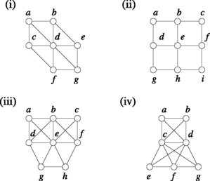
• 5. List all Hamiltonian cycles in the graphs shown.

  

• 6. Consider a complete graph K ₅ with vertices abcde, the costs associated with the edges being

  $$\begin{array}{l@{\qquad}l@{\qquad}l@{\qquad}l@{\qquad}l}ab=1, & ac=2, & ad=3, &ae=4, & bc=7, \\bd=8, & be=9, & cd=5, & ce=6, & de=10.\end{array} $$

  Find the cost of the cheapest Hamiltonian cycle in this graph by a complete search. Then find the costs of the routes generated by the nearest neighbor algorithm starting at each of the five vertices in turn and show that the nearest neighbor solution is never the cheapest.

• 7. In the following problems you are given the costs associated with the edges of a complete graph with vertices abcde. Find the costs of the routes generated by the nearest neighbor algorithm starting at each of the five vertices in turn and by the sorted edges algorithm.

  • (i) $\begin{array}[t]{rcl@{\qquad}l@{\qquad}l@{\qquad}l@{\qquad}l}ab&=&24, & ac=26, & ad=20, &ae=21, & bc=33, \\bd&=&29, & be=30, & cd=25, & ce=27, & de=28;\end{array}$

  • (ii) $\begin{array}[t]{rcl@{\qquad}l@{\qquad}l@{\qquad}l@{\qquad}l}ab&=&59, & ac=69, & ad=60, &ae=58, & bc=56, \\bd&=&69, & be=54, & cd=58, & ce=66, & de=61;\end{array}$

  • (iii) $\begin{array}[t]{rcl@{\qquad}l@{\qquad}l@{\qquad}l@{\qquad}l}ab&=&16, & ac=24, & ad=30, &ae=48, & bc=27, \\bd&=&29, & be=44, & cd=16, & ce=46, & de=51;\end{array}$

  • (iv) $\begin{array}[t]{rcl@{\qquad}l@{\qquad}l@{\qquad}l@{\qquad}l}ab&=&91, & ac=79, & ad=75, &ae=82, & bc=87, \\bd&=&64, & be=78, & cd=68, & ce=81, & de=88;\end{array}$

  • (v) $\begin{array}[t]{rcl@{\qquad}l@{\qquad}l@{\qquad}l@{\qquad}l}ab&=&45, & ac=28, & ad=50, &ae=36, & bc=21, \\bd&=&42, & be=34, & cd=44, & ce=39, & de=25;\end{array}$

  • (vi) $\begin{array}[t]{rcl@{\qquad}l@{\qquad}l@{\qquad}l@{\qquad}l}ab&=&11, & ac=15, & ad=13, &ae=18, & bc=20, \\bd&=&12, & be=16, & cd=14, & ce=19, & de=17;\end{array}$

  • (vii) $\begin{array}[t]{rcl@{\qquad}l@{\qquad}l@{\qquad}l@{\qquad}l}ab&=& 14, & ac=12, & ad=15, &ae=24, & bc=27, \\bd&=&29, & be=44, & cd=16, & ce=46, & de=51;\end{array}$

  • (viii) $\begin{array}[t]{rcl@{\qquad}l@{\qquad}l@{\qquad}l@{\qquad}l}ab&=&44, & ac=49, & ad=56, &ae=52, & bc=45, \\bd&=&54, & be=48, & cd=51, & ce=55, & de=50.\end{array}$

• 8. Prove that the following graph contains no Hamiltonian cycle.

  

4.7 Graph Representations and Colorings

4.7.1 Representations and Crossings

Consider these two diagrams.

They represent the same graph, the complete graph K ₄ on four vertices. But as diagrams they are quite different: in the left-hand version, two edges cross; in the right-hand diagram there are no crossings. We shall refer to the two diagrams as different representations of K ₄ in the plane. The crossing number of a representation is the number of different pairs of edges that cross; the crossing number ν(G) of a graph G is the minimum number of crossings in any representation of G. The diagram shows representations of K ₄ with crossing numbers 1 and 0, respectively. As one cannot have a representation with fewer than 0 crossings, we have shown that ν(K ₄)=0.

A representation is called planar if it contains no crossings, and a planar graph is a graph that has a planar representation. In other words, a planar graph G is one for which ν(G)=0. So K ₄ is planar.

There are many applications of crossing numbers. An early use was in the design of railway yards, where it is inconvenient to have the different lines crossing, and it is better to have longer track rather than extra intersections. An obvious extension of this idea is freeway design. At a complex intersection, fewer crossings will mean fewer expensive flyover bridges. More recently, small crossing numbers have proven important in the design of VLSI chips; if two parts of a circuit are not to be connected electrically, but they cross, a costly insulation process is necessary.

Surprisingly enough, the crossing numbers of complete graphs are not easy to calculate. A very easy (but very bad) upper bound can be found as follows. If the v vertices of K _v are arranged in a circle, and all the edges are drawn as straight lines, then every set of four vertices contributes exactly one crossing. So

$$\nu(K_v) \le C(v,4).$$

More sophisticated constructions can be used to find better upper bounds, but the exact answer is not known in general.

Sample Problem 4.25

Prove that the crossing number of the complete graph on five vertices is 1.

Solution

We start by considering smaller complete graphs. The representation of K ₃ as a triangle is essentially unique: one can introduce a crossing only by a fanciful, twisting representation of one or more edges. Adding one more vertex to obtain a K ₄, one always obtains a representation like the left-hand diagram we saw at the start of the section, and any other planar representation is essentially equivalent to this. So any planar representation of K ₅ can be obtained by introducing another vertex into this representation of K ₄. If a new vertex e is introduced inside the triangle abd, then the representation of ce must cross one of ab, ad, or bd. Similarly, the introduction of e inside any triangle causes a crossing involving the edge joining e to the vertex that is not on the triangle. (The “outer area” is considered to be the triangle abc.) The following diagrams illustrate this for the triangles abc and abc.

Therefore, ν(K ₅)≥1. A representation with one crossing is easy to find—we have found three of them already—so ν(K ₅)=1.

Your Turn

Prove that the crossing number of the complete bipartite graph K _3,3 is 1.

It is easy to calculate the crossing numbers of some small graphs. For example, the crossing number of any tree is 0. To see this, simply draw the tree as a tree diagram, as we did in Section 4.5. The diagram has no crossings. Similarly, any cycle has crossing number 0.

Suppose G is planar. If a new graph were constructed by inserting a new vertex of degree 2 into the middle of an edge (dividing an edge), or by deleting a vertex of degree 2 and joining the two vertices adjacent to it (eliding a vertex), that new graph will also be planar. Graphs that can be obtained from each other in this way are called homeomorphic.

As K ₅ and K _3,3 are not planar, it follows that a graph having either as a subgraph could not be planar. Moreover, a graph that is homeomorphic to one with a subgraph homeomorphic to K ₅ or K _3,3 cannot be planar. In fact, it may be shown that this necessary condition for planarity is also sufficient. The proof is too difficult for our purposes.

Theorem 15

G is planar if and only if G is homeomorphic to a graph containing no subgraph homeomorphic to K ₅ or K _3,3.

4.7.2 Maps and Planarity

By a map we shall mean what is usually meant by a map of a continent (showing countries) or a country (showing states or provinces). However, we shall make one restriction. Sometimes one state can consist of two disconnected parts (in the United States, Michigan consists of two separate land masses, unless we consider man-made constructions such as the Mackinaw Bridge). We shall exclude such cases from consideration.

Given a map, we can construct a graph as follows: the vertices are the countries or states on the map, and the two vertices are joined by an edge precisely when the corresponding countries have a common border.

Sample Problem 4.26

Represent the map of the mainland of Australia, divided into states and the Northern Territory, as a graph.

Solution

The map is shown, for reference, alongside its graph.

Vertex T represents the Northern Territory; the states (New South Wales, Queensland, South Australia, Victoria, and Western Australia) are denoted by their initials.

Your Turn

Represent the map of the New England states—Maine, New Hampshire, Massachusetts, Vermont, Connecticut, Rhode Island—as a graph.

Sometimes two states have only one point in common. An example, in the United States, occurs where Utah and New Mexico meet at exactly one point, as do Colorado and Arizona. We shall say that states with only one point in common have no border, and treat them as if they do not touch.

It is always possible to draw the graph corresponding to a map without crossings. To see this, draw the graph on top of the map by putting a vertex inside each state and joining vertices by edges that pass through common state borders so the graph of any map is planar. Conversely, any planar graph is easily represented by a map. Therefore, the theory of maps (with the two stated restrictions) is precisely the theory of planar graphs.

In 1852, William Rowan Hamilton wrote to Augustus de Morgan concerning a problem that had been posed by a student, Frederick Guthrie. Guthrie said: cartographers know that any map (our definition) can be colored using four or less colors; is there a mathematical proof? (Guthrie later pointed out that the question had come from his brother, Francis Guthrie.)

Kempe published a purported proof in 1879. It was thought that the matter was over, but in 1890 Heawood pointed out a fallacy in Kempe’s proof. Heawood did, however, repair the proof sufficiently to prove that every planar map can be colored in five colors.

After Heawood’s paper appeared, there was renewed interest in the four-color problem. Because it was easy to state and tantalizingly difficult to prove, it became one of the most celebrated unsolved problems in mathematics. In 1976, Appel and Haken finally proved that any map can be colored in at most four colors. Their proof involved computer analysis of a large number of cases, so many that human analysis of all the cases is not feasible. We state their theorem as

Theorem 16

(The Four-Color Theorem)

Every map can be colored using at most four colors.

4.7.3 Graph Colorings

Instead of coloring a map, we could instead apply the colors to the vertices of the corresponding graph. The result to divide the set of vertices into disjoint subsets, where each subset consists of the vertices that receive a specific color. The defining property is that no two elements of the same subset are adjacent. The terminology of colors and colorings is traditionally used for this sort of problem. Given a set C={c ₁,c ₂,…} is a set of labels called colors, a C-coloring (or C-vertex coloring) ξ of a graph G is a function

$$\xi: V(G) \to C,$$

that is, a rule that assigns a uniquely-defined color to each vertex. The sets V _i ={x:ξ(x)=c _i } are called color classes. A proper coloring of G is a coloring in which no two adjacent vertices belong to the same color class. In other words,

$$x \sim y \quad \Rightarrow\quad \xi(x) \ne\xi(y).$$

A proper coloring is called an n-coloring if C has n elements. If G has an n-coloring, then G is called n-colorable. So the Four-Color Theorem says that every planar graph is 4-colorable.

The chromatic number χ(G) of a graph G is the smallest integer n such that G has an n-coloring. A coloring of G in χ(G) colors is called minimal. We use the phrase “G is n-chromatic” to mean that χ(G)=n (but note that a minority of authors use n-chromatic as a synonym for n-colorable).

Some easy small cases of chromatic number are

A cycle of length v has chromatic number 2 if v is even and 3 if v is odd. The star K _1,n has chromatic number 2; this is an example of the next theorem.

Clearly, χ(G)=1 if G has no edges and χ(G)=2 if G has at least one edge.

Suppose G is a graph with a subgraph H, and suppose G has been n-colored. If all the vertices and edges that are not in H were deleted, there would remain a copy of H that is colored in at most n colors. So χ(H)≤χ(G) whenever H is a subgraph of G.

The graph of Figure 4.13 can be colored in three colors:

$$V_0 = \{ x_1, x_4 \},\qquad V_1= \{ x_2, x_5 \},\qquad V_2 = \{x_3, x_6 \}.$$

Fig. 4.13

A graph with chromatic number 3

Exercises 4.7 A

• 1. Which of the following graphs are planar?

  

• 2. For each of the following graphs, find the chromatic number and find a coloring that uses the minimum number of colors.

  

• 3. Find the chromatic number and find a coloring that uses the minimum number of colors for the graphs in Exercise 1, parts (v) and (vi).

• 4. The wheel W _n was defined in Exercise 4.3A.5 to consist of an n-cycle together with a further vertex adjacent to all n vertices. What is χ(W _n )?

• 5. Verify that there are exactly three connected incomplete graphs on four vertices with maximum degree 3, and all can be 3-colored.

• 6. G is formed from the complete graph K _v by deleting one edge. Prove that χ(G)=v−1 and describe a way of coloring G in v−1 colors.

Exercises 4.7 B

• 1. Which of the following graphs are planar?

  

• 2. Prove that ν(K _1,n )=ν(K _2,n )=0 for any n.

• 3. Prove that ν(K _3,3)=1. What is ν(K _3,4)?

• 4. In Sample Problem 4.26, we drew the graph corresponding to a map of Australia, but omitted the Australian Capital Territory (A.C.T.) and Tasmania. Draw the graph that would result if these two areas were included. (For your information, the A.C.T. lies wholly within New South Wales, and Tasmania is an island to the south.) What is the chromatic number?

• 5. Find the crossing numbers of the following graphs.

  

  For each graph in the preceding question, find the chromatic number and find a coloring that uses the minimum number of colors.

• 6. G is the union of two graphs G ₁ and G ₂ that have one common vertex. Show that χ(G)=max{χ(G ₁),χ(G ₂)}.

• 7. For each of the following graphs, find the chromatic number and find a coloring that uses the minimum number of colors.

  

• 8. Write P for the Petersen graph, which was defined in Exercise 4.3A.9

  • (i) What is χ(P)?

  • (ii) Prove that P is not planar. What is its crossing number?