Holling II predator–prey impulsive semi-dynamic model with complex Poincaré map

Abstract

Planar impulsive semi-dynamic systems arising biological applications including integrated pest management have been paid great attention recently. However, most of works only focus on very special cases of proposed models, and the complete dynamics are far from being resolved due to complexity. Therefore, a planar impulsive Holling II prey–predator semi-dynamic model has been employed with aims to develop analytical techniques and provide a comprehensive qualitative analysis of global dynamics for whole parameter space. To do this, we initially assume that the proposed ODE model does not exist positive steady state. We determine the Poincaré map for impulsive point series defined in the phase set and analyze its properties including monotonicity, continuity, discontinuity and convexity. We address the existence, local and global stability of an order-1 limit cycle and obtain sharp sufficient conditions for the global stability of the boundary order-1 limit cycle. Moreover, the existence of an order-3 limit cycle indicates that the proposed model exists any order limit cycles. If the proposed ODE model exists an unstable focus, then the results show that a finite or an infinite countable discontinuity points for the Poincaré map imply the model exists a finite or an infinite number of order-1 limit cycles. The bifurcation analyses show that the model undergoes a transition to chaos via a cascade of period-adding bifurcation and also multiple attractors can coexist.

1 Introduction

Impulsive semi-dynamical system is widely used to model biological systems with threshold control strategy, such as biological resource and pest management programmes, and chemostat cultures in ecological systems [24, 29, 34–37, 39, 40], virus dynamical systems (HIV) [26, 41, 48, 50, 51], diabetes mellitus and tumor control in pharmacological systems [18, 23, 42], vaccination strategies and epidemiological control in epidemiology [16, 31, 32, 43, 49]. These systems involve an interacting mixture of continuous and discrete dynamics exhibiting discontinuity on appropriate manifolds, which are called as impulsive sets and hence give rise to impulsive dynamics [2, 4, 19–21].

Recently, the qualitative theory for impulsive semi-dynamical system has been developed extensively, and the analytical techniques include the Lyapunov method [24, 34, 36, 37, 39, 40], invariant and limiting sets [5, 7–10, 27], the LaSalle’s invariance principle [6] and the Poincaré–Bendixson theorem [8, 52]. Moreover, some prototype models with biological motivations have been proposed and investigated with aims to guide the development of a general qualitative theory of semi-dynamical systems [34, 36, 37, 39, 40].

State-dependent feedback control strategy can be defined in broad terms in real biological problems, which is usually modeled by an impulsive semi-dynamical system. For example, control tactic (grazing, harvesting, pesticide application, treatment, etc.) is implemented only when a specific species abundance reaches a previously given threshold density. In particular, a good example in the series of models motivated by integrated pest management (IPM) [34, 36, 39, 40] has been formulated and investigated. Note that IPM is a long-term management strategy that uses a combination of biological, cultural and chemical tactics to reduce pests to tolerable levels, control tactics must be taken once a critical density of pests (economic threshold, ET) is observed in the field so that the economic injury level (EIL) is not exceeded [34, 40, 46, 47].

For the model with IPM strategy [34, 40], the classical Lotka–Volterra system with state-dependent feedback control is used, and some novel techniques are developed to examine the existence and stability of an order-1 limit cycle, nonexistence of limit cycles with order no less than 3, the coexistence of multiple attractors and their basins of attraction. Liu et al. [25] have extended those methods to study the Holling II predator–prey model with IPM under which the model exits a stable focus, and similar results have been obtained. Recently, the modeling framework and the developed analytical techniques in [34, 40] have been used in a number of recent studies. For example, Huang et al. [18] proposed mathematical models depicting impulsive injection of insulin for type 1 and type 2 diabetes mellitus and considered the existence and local stability of an order-1 limit cycle. When considering the biomass concentration as an index, chemostat models with state-dependent feedback control have been proposed and analyzed in [29, 33, 45]. The work [43] also considered the existence and stability of limit cycles with different orders, in relation to the biological issue of maintaining the density of infected plant population below a certain threshold level. See also similar work on population dynamics [28, 44, 52] and epidemiology [43].

Based on the properties of the successor function and the Poincaré map, the existence and local stability of the order-1 periodic solution have been addressed in the above-mentioned work. One common assumption in those papers is that any solution initiating from the phase set must experience infinite many impulses. Further, if the proposed model exists a first integral [34, 40], the existence of the order-2 periodic solutions and other rich dynamics can be discussed in more detail. Even so the global dynamics of proposed models with state-dependent feedback control arising from modeling IPM and other fields are far from being solved [25, 34, 36, 39, 40]. The challenge for investigating the global dynamics remains due to the state-dependent impulsive control and the complexity of the Poincaré map. For example, the Poincaré map still includes several discontinuous points even if any solution starting from phase set experiences infinitely many impulsive effects (see more details from the main text). Moreover, a more and more extensive applications in the wide fields require much more advanced qualitative techniques and new methods to reveal complete dynamics of the proposed model with threshold control policy and consequently to discuss the biological implications.

The main purpose of this study is to develop analytical techniques and provide a comprehensive qualitative analysis of the global dynamics through analyzing a planar impulsive Holling II prey–predator semi-dynamic model. To do this, we firstly examine the properties of the Poincaré map for impulsive point series defined in the phase set including monotonicity, continuity, discontinuity and convexity. The existence, local and global stability of an order-1 limit cycle have been addressed and sharp sufficient conditions for the global stability of the boundary order-1 limit cycle are obtained. Moreover, the existence of an order-3 limit cycle indicates that the proposed model exists any order limit cycles. An infinite countable discontinuity points for the Poincaré map imply the model may exist an infinite number of order-1 limit cycles, and the bifurcation analyses show that the model undergoes a transition to chaos via a cascade of period-adding bifurcation and also multiple attractors can coexist. All the results can help us to further understand and give insight into the qualitative theory and the dynamic complexity of impulsive semi-dynamical system.

2 The model with state-dependent feedback control

The basic ODE model employed in this work is the following classical Holling II predator–prey model [38]

$$\begin{aligned} \left\{ \begin{array}{l} \displaystyle \frac{\hbox {d}x(t)}{\hbox {d}t}= rx(t)\left[1-\frac{x(t)}{K}\right] -\frac{\beta x(t)y(t)}{1+\omega x(t)}, \\ \displaystyle \frac{\hbox {d}y(t)}{\hbox {d}t}= \displaystyle \frac{\eta \beta x(t)y(t)}{1+\omega x(t)}-\delta y(t),\\ \end{array}\right. \end{aligned}$$

(1)

where $x(t)$ and $y(t)$ represent the densities of prey (pest) and predator (natural enemy), respectively, $r$ is the intrinsic growth rate of the prey population and $K$ represents its carrying capacity, ${(\beta x(t))}/({1+\omega x(t)})$ denotes the Holling II functional response, which is a saturating function of the amount of pest present, and $\delta$ denotes the death rate of the predator population.

Model (1) always exists a $(0, 0)$ steady state, which is unstable and a boundary equilibrium $(K,0)$. The positive steady state

$$\begin{aligned} E^*=(x_e,y_e)=\left( \frac{\delta }{\eta \beta -\delta \omega }, \frac{r\eta (K\eta \beta -K\delta \omega -\delta )}{K(\eta \beta -\delta \omega )^2}\right) \end{aligned}$$

exists provided

$$\begin{aligned} \eta \beta -\delta \omega >\delta /K\Leftrightarrow R_0\doteq \frac{K[\eta \beta -\delta \omega ]}{\delta }>1. \end{aligned}$$

Moreover, if $R_0\le 1$, then $(K, 0)$ is globally stable, and if $R_0>1$, then $(K,0)$ becomes unstable. Further, if

$$\begin{aligned} \omega K\le \frac{\eta \beta +\omega \delta }{\eta \beta -\omega \delta }\Leftrightarrow R_1\doteq \frac{\eta \beta +\omega \delta }{\eta \beta -\omega \delta }\frac{1}{\omega K}\ge 1, \end{aligned}$$

then $E^*$ is a globally stable node or focus. Otherwise, it is an unstable node or focus, and model (1) has a unique limit cycle which is stable.

The eigenfunction at $E^*$ is as follows

$$\begin{aligned}&\lambda ^2-\frac{r\delta (-\beta \eta +K\beta \eta \omega -K\delta \omega ^2-\delta \omega )}{K\beta \eta (\beta \eta -\delta \omega )}\lambda \nonumber \\&\quad +\frac{r\delta (K\beta \eta -K\delta \omega -\delta )}{K\beta \eta }=0, \end{aligned}$$

i.e., we have

$$\begin{aligned} \lambda ^2-\frac{C_3 C_1}{C_0}\lambda +C_3 C_2=0 \end{aligned}$$

with $C_0=\beta \eta -\delta \omega ,\, C_1=-\beta \eta +K\omega \xi -\delta \omega , C_2=K\xi -\delta$ and $C_3={(r\delta )}/({K\beta \eta })$. Therefore, we denote

$$\begin{aligned} \triangle =\left(\frac{C_3 C_1}{C_0}\right)^2-4C_3 C_2. \end{aligned}$$

Two isoclines can be defined as follows:

$$\begin{aligned} L_1: y\!=\!\frac{r}{\beta }\left[1\!-\!\frac{x}{K}\right](1\!+\!\omega x), \hbox {and}\ L_2: x\!=\!\frac{\delta }{\eta \beta \!-\!\delta \omega }. \end{aligned}$$

Now, we take the integrated control tactics into account for model (1). Once the density of the pest population reaches the ET, impulsive reduction in its density is possible after its partial destruction by trapping or by poisoning with chemicals, and an impulsive increase in a controlling predator or parasitoid population density is possible by artificial breeding and releases [3, 34, 40]. Then, model (1) becomes

$$\begin{aligned} \left\{ \begin{array}{l} \left. \begin{array}{l} \displaystyle \frac{\hbox {d}x(t)}{\hbox {d}t}\!=\! rx(t)\left[1\!-\!\frac{x(t)}{K}\right] \!-\!\frac{\beta x(t)y(t)}{1\!+\!\omega x(t)}, \\ \displaystyle \frac{\hbox {d}y(t)}{\hbox {d}t}= \displaystyle \frac{\eta \beta x(t)y(t)}{1+\omega x(t)}-\delta y(t),\\ \end{array}\right\} \quad x\!<\!\hbox {ET}, \\ \left. \begin{array}{l} x(t^+)= (1-\theta )x(t), \\ y(t^+)= y(t)+\tau ,\\ \end{array}\right\} \quad x=\hbox {ET},\\ \end{array}\right. \end{aligned}$$

(2)

where $x(t^+)\doteq x^+$ and $y(t^+)\doteq y^+$ denote the numbers of pests and natural enemies after an integrated control strategy is applied at time $t$, and $x(0^+)$ and $y(0^+)$ denote the initial densities of pest and natural enemy populations. Throughout this paper, we assume that the initial density of the pest population is always less than $ET$ (i.e., $x(0^+)\doteq x_0^+<ET, \quad y(0^+)\doteq y_0^+>0$) and $ET<K$. Otherwise, the initial values are taken after an integrated control strategy application. In model (2), $0\le \theta <1$ is the proportion by which the pest density is reduced by killing and/or trapping once the number of pests reaches $ET$, while $\tau$ ($\tau \ge 0$) is the constant number of natural enemies released at this time $t$.

The above model can be defined as an impulsive semi-dynamic system in the sense that it is defined by both a continuous and a discrete event. This structure makes the model very interesting and complexity. Note that this model has been investigated recently [25], but the authors only focused on the very special case, i.e., model (1) has a global stable equilibrium $E^*$, which cannot reveal the rich dynamics. Indeed, the state-dependent feedback control to the classical Holling II predator–prey model will result in rich dynamic behaviors, which cannot appear in model (1), including multiple limit cycles, period-adding bifurcations and chaotic solutions. Thus, in this work we would like to rigorously address these different behaviors from a mathematical point of view. To do this, we first introduce some basic definitions and preliminaries related to impulsive semi-dynamic system, which are useful throughout this work.

3 Planar impulsive semi-dynamic systems and preliminaries

The generalized planar impulsive semi-dynamical systems with state-dependent feedback control can be described as follows:

$$\begin{aligned} \left\{ \begin{array}{l} \begin{array}{l} \displaystyle \frac{\hbox {d}x}{\hbox {d}t}= P(x, y),\quad \displaystyle \frac{\hbox {d}y}{\hbox {d}t}= Q(x,y),\\ \end{array}\quad (x,y)\notin {\mathcal {M}},\\ \begin{array}{l} \triangle x=a(x,y), \quad \triangle y=b(x,y), \end{array}\quad (x,y)\in {\mathcal {M}}, \end{array}\right. \end{aligned}$$

(3)

where $(x, y)\in R^2,\, \triangle x=x^+-x$ and $\triangle y=y^+-y$. $P, Q, a, b$ are continuous functions from $R^2$ into $R,\, {\mathcal {M}}\subset R^2$ denotes the impulsive set. For each point $z(x,y)\in {\mathcal {M}}$, the map or impulsive function $I: R^2\rightarrow R^2$ is defined as

$$\begin{aligned}&I(z) = z^+=(x^+, y^+)\in R^2,\, x^+=x+a(x,y), \\&y^+= y+b(x,y) \end{aligned}$$

and $z^+$ is called as an impulsive point of $z$.

Let ${\mathcal {N}}=I({\mathcal {M}})$ be the phase set (i.e., for any $z\in {\mathcal {M}}, I(z)=z^+\in {\mathcal {N}}$), and ${\mathcal {N}}\cap {\mathcal {M}}=\emptyset$. Let $(X, {\varPi }, R_+)$ or $(X, {\varPi })$ be a semi-dynamical system [1], where $X=R^2$ is a metric space, $R_+$ is the set of all nonnegative reals. For any $z\in X$, the function ${\varPi }_z: R_+\rightarrow X$ defined by ${\varPi }_z(t)={\varPi }(z, t)$ is clearly continuous such that ${\varPi }(z,0)=z$ for all $z\in X$, and ${\varPi }({\varPi }(z,t),s)={\varPi }(z,t+s)$ for all $z\in X$ and $t,s\in R_+$. The set

$$\begin{aligned} C^+(z)=\{{\varPi }(z,t)| t\in R_+\} \end{aligned}$$

is called the positive orbit of $z$. For all $t\ge 0$ and $z\in X$, we define $F(z,t)=\{w: {\varPi }(w,t)=z\}$, and further for any set ${\mathcal {M}} \subset X$, let

$$\begin{aligned} {\mathcal {M}} ^+(z)=C^+(z)\cap {\mathcal {M}} -\{z\}. \end{aligned}$$

Based on above notations, we now provide the definitions of impulsive semi-dynamic system and order-$k$ periodic solution as follows [8, 11–13, 19, 20, 22].

Definition 1

An planar impulsive semi-dynamic system $(R^2, {\varPi }; {\mathcal {M}}, I)$ consists of a continuous semi-dynamic system $(R^2, {\varPi })$ together with a nonempty closed subset ${\mathcal {M}}$ (or impulsive set) of $R^2$ and a continuous function $I: {\mathcal {M}}\rightarrow R^2$ such that for every $z\in {\mathcal {M}}$, there exists a $\epsilon _z>0$ such that

$$\begin{aligned}F(z, (0, \epsilon _z))\cap {\mathcal {M}}=\emptyset \ \mathrm {and}\ {\varPi }(z, (0, \epsilon _z))\cap {\mathcal {M}}=\emptyset .\end{aligned}$$

Throughout the paper, we denote the points of discontinuity of ${\varPi }_z$ by $\{z^+_n\}$ and call $z_n^+$ an impulsive point of $z_n$. We define a function ${\varPhi }$ from $X$ into the extended positive reals $R_+\cup \{\infty \}$ as follows: let $z\in X$, if ${\mathcal {M}}^+(z)=\emptyset$ we set ${\varPhi }(z)=\infty$, otherwise ${\mathcal {M}}^+(z)\ne \emptyset$ and we set ${\varPhi }(z)=s$, where ${\varPi }(z,t)\notin {\mathcal {M}}$ for $0<t<s$ but ${\varPi }(z,s)\in {\mathcal {M}}$.

Definition 2

A trajectory ${\varPi }_z$ in $(R^2, {\varPi }, M, I)$ is said to be periodic of period $T_k$ and order $k$ if there exist nonnegative integers $m\ge 0$ and $k\ge 1$ such that $k$ is the smallest integer for which $z_m^+=z_{m+k}^+$ and $T_k=\sum \nolimits _{i=m}^{m+k-1}{\varPhi }(z_i)=\sum \nolimits _{i=m}^{m+k-1}s_i$.

For more details of the concepts and properties of continuous semi-dynamic systems and impulsive semi-dynamic systems, see [1, 8, 19, 27, 53] for more details. For simplicity, we denote a periodic trajectory of period $T_k$ and order-$k$ by an order- $k$ periodic solution. An order-$k$ periodic solution is called as an order- $k$ limit cycle if it is isolated. The local stability of an order-$k$ periodic solution can be determined by using following analogue of Poincaré criterion [30].

Lemma 1

Let $\phi (x,y)$ be a sufficiently smooth function with $\mathrm {grad}\phi (x,y)\ne 0$, and we denote $\phi (x,y)\ne 0$ as $(x,y)\notin {\mathcal {M}}$ and $\phi (x,y)=0$ as $(x,y)\in {\mathcal {M}}$. The order-$k$ periodic solution $x=\xi (t), y=\eta (t)$ of model (3) is orbitally asymptotically stable and enjoys the property of asymptotic phase if the multiplier $\mu _2$ satisfies the condition $|\mu _2|<1$. Where

$$\begin{aligned}&\mu _2 \!=\! \prod \limits _{k=1}^{q}\triangle _k \mathrm{exp}\left[ \int _0^T\left( \frac{\partial P}{\partial x}(\xi (t),\eta (t)) \!+\!\frac{\partial Q}{\partial y}(\xi (t),\eta (t))\right) \mathrm{d}t\right] , \\&\triangle _k \!=\! \frac{P_+\left( \frac{\partial b}{\partial y}\frac{\partial \phi }{\partial x}\!-\!\frac{\partial b}{\partial x} \frac{\partial \phi }{\partial y}\!+\!\frac{\partial \phi }{\partial x}\right) + Q_+\left( \frac{\partial a}{\partial x}\frac{\partial \phi }{\partial y}\!-\!\frac{\partial a}{\partial y} \frac{\partial \phi }{\partial x}\!+\!\frac{\partial \phi }{\partial y}\right) }{P\frac{\partial \phi }{\partial x}\!+\! Q\frac{\partial \phi }{\partial y}}, \end{aligned}$$

and $P, Q, ({\partial a})/({\partial x}),({\partial a})/({\partial y})$, $({\partial b})/({\partial x})$, $({\partial b})/ ({\partial y}), ({\partial \phi })/({\partial x})$, $({\partial \phi })/({\partial y})$ are calculated at the point $(\xi (\tau _k),\eta (\tau _k))$ and $P_+=P(\xi (\tau _k^+), \eta (\tau _k^+))$, $Q_+=Q(\xi (\tau _k^+),\,\eta (\tau _k^+))$ with $\tau _k^+={\varPhi }(\xi (\tau _{k-1}^+),\eta (\tau _{k-1}^+))$.

It is interesting to know as well that given $z\in R^2$, one of the three properties for the positive orbits of model (3) or planar impulsive semi-dynamic system holds:

• ${\mathcal {M}}^+(z)={\mathcal {M}}^+(z_0^+)=\emptyset$, and thus, the orbit of $z_0^+$ has no discontinuities, i.e., it is completely determined by the corresponding orbit of ODE model.

• There exists a positive integer $n$ such that $z_k^+$ is defined for any $k=1,2, \ldots ,n,\, {\mathcal {M}}^+(z_k^+)\ne \emptyset$ for $k<n$ and ${\mathcal {M}}^+(z_n^+)= \emptyset$. In this case, the trajectory of $z$ exists a finite number of discontinuities, i.e., the trajectory experiences finitely many impulses.

• If for any $k\ge 1,\, z_k^+$ is defined and ${\mathcal {M}}^+(z_k^+)\ne \emptyset$, then the trajectory of $z$ has infinitely many discontinuities, i.e., the trajectory experiences infinitely many impulses.

4 Poincaré map and its properties

In order to address the dynamic behavior of system (2), we first construct a Poincaré map determined by the impulsive points in phase set. From a biological point of view, we focus on the space $R_+^2=\{(x,y): x\ge 0, y\ge 0\}$ to investigate model (2).

4.1 Impulsive semi-dynamic system defined by model (2)

Define two straight lines as follows:

$$\begin{aligned} L_3: x=(1-\theta )\hbox {ET}; \, \, \text {and} \, \, L_4: x=\hbox {ET}. \end{aligned}$$

According to the fact of $0<\hbox {ET}<K$ and substituting $x=\hbox {ET}$ into the line $L_1$, one yields the intersection point of two lines $L_1$ and $L_4$, denoted by $Q_\mathrm{ET}=(\hbox {ET}, y_\mathrm{ET})$ with

$$\begin{aligned} y_\mathrm{ET}=\frac{r}{\beta }\left[1-\frac{\hbox {ET}}{K}\right](1+\omega \hbox {ET}). \end{aligned}$$

Similarly, we denote the intersection point of two lines $L_1$ and $L_3$ as $Q_{\theta \hbox {ET}}=((1-\theta )\hbox {ET}, y_{\theta \mathrm{ET}})$ with

$$\begin{aligned} y_{\theta \mathrm{ET}}=\frac{r}{\beta }\left[1-\frac{(1-\theta )\hbox {ET}}{K}\right](1+\omega (1-\theta ) \hbox {ET}). \end{aligned}$$

Define the open set in $R_+^2$ as follows

$$\begin{aligned} {\varOmega }=\{(x,y)| x>0, y> 0, x<\hbox {ET}\}\subset R_+^2. \end{aligned}$$

(4)

To address the exact domains of the impulsive sets and phase sets and consequently define the impulsive semi-dynamic system for model (2), based on the existence and stability of the steady state $E^*$ of model (1), we consider the following three cases:

$$\begin{aligned}&(C_1): \, R_0\le 1; \quad (C_2): \, R_0>1 \, \mathrm {and}\, R_1< 1;\\&(C_3):\, \, R_0>1 \, \mathrm {and}\, R_1\ge 1. \end{aligned}$$

For case $(C_1)$, the interior equilibrium $E^*$ does not exist, and there are two feasible equilibria $(0, 0)$ which is an unstable saddle and $(K, 0)$ which is globally stable in first quadrant. This indicates that any solution of model (1) initiating from ${\varOmega }$ will reach at the line $L_4$ in a finite time. Now we can define the impulsive set ${\mathcal {M}}$ of model (2)

$$\begin{aligned} \mathcal {M}=\{(x,y)|\ x=\hbox {ET}, 0\le y\le y_\mathrm{ET}\}, \end{aligned}$$

(5)

which is a closed subset of $R_+^2$. Define the continuous function $I: (\hbox {ET}, y)\in {\mathcal {M}}\rightarrow (x^+,y^+)=((1-\theta )\hbox {ET}, y+\tau )\in {\varOmega }$. Thus, the phase set ${\mathcal {N}}$ can be defined as follows

$$\begin{aligned} {\mathcal {N}}= & {} I({\mathcal M})=\left\{ (x^+, y^+)\in {\varOmega }|\ x^+=(1-\theta )\hbox {ET}, \right. \nonumber \\&\left. \tau \le y^+\le y_\mathrm{ET}+\tau \right\} \doteq \left\{ (x^+,y^+)\in {\varOmega }|\ x^+\right. \nonumber \\&\left. =(1-\theta )V_L, y^+\in Y_D\right\} \end{aligned}$$

(6)

with $Y_D\!=\!\left[\tau , y_\mathrm{ET}+\tau \right]$. Therefore, $(R_+^2, {\varPi }; {\varOmega }, \mathcal {M}, I)$ or $(R_+^2, {\varPi }; \mathcal {M}, I)$ with respect to model (2) defines an impulsive semi-dynamic system.

Unless otherwise specified in the following, we assume the initial point $(x_0^+, y_0^+)\in {\mathcal {N}}$. For convenience in defining the Poincaré map, we use $Y_D=\left[\tau , +\infty \right)$ in the rest work due to any solution of model (2) initiating from $(x_0^+, y_0^+)$ with $y_0^+>y_\mathrm{ET}+\tau$ will satisfy $y_k^+\le y_\mathrm{ET}+\tau$ for all $k\ge 1$.

Note that for case $(C_2)$, there exists a unique stable limit cycle of model (1), denoted by ${\varGamma }_{(1)}$, which intersects with the isocline $L_1$ at two points $E_{{\varGamma }_1}(x_{{\varGamma }_1}, y_{{\varGamma }_1})$ and $E_{{\varGamma }_2}(x_{{\varGamma }_2}, y_{{\varGamma }_2})$ with $x_{{\varGamma }_1}<x_{{\varGamma }_2}$. Therefore, any solution starting from $((1-\theta )\hbox {ET}, y_0^+)$ with $y_0^+\ge 0$ will experience infinitely many impulses for case $(C_2)$ provided $\hbox {ET}\le x_{{\varGamma }_2}$ and case $(C_3)$ provided $\hbox {ET}<x_e$. Otherwise, any solution starting from $((1-\theta )\hbox {ET}, y_0^+)$ with $y_0^+\ge 0$ may be free from pulse effect or experiences finitely (infinitely) many impulses which depends on the initial conditions. Therefore, the impulsive sets and phase sets of model (2) could vary, which will result in complex dynamics for model (2) under cases $(C_2)$ and $(C_3)$, and we will address those in next section.

4.2 Poincaré map and its properties for case $(C_1)$

The Poincaré map of model (2) could be defined in different ways, and all of them are useful for investigating the dynamics of model (2).

Define two sections as follows:

$$\begin{aligned}&S_\mathrm{ET}= \Big \{(x,y)| x = \hbox {ET}, y\ge 0\Big \}, \\&S_{\theta \hbox {ET}}= \Big \{(x,y)| x=(1-\theta )\hbox {ET}, \quad y\ge 0\Big \}. \end{aligned}$$

Choosing the section $S_{\theta \mathrm{ET}}$ as a Poincaré section. Assume that the point $P_{k}^+=((1-\theta )\hbox {ET}, y_k^+)$ lies in the section $S_{\theta \mathrm{ET}}$, and the trajectory ${\Psi }(t,t_0,(1-\theta )\hbox {ET},y_k^+)\doteq (x(t,t_0,(1-\theta )\hbox {ET},y_k^+),y(t,t_0,(1-\theta )\hbox {ET},y_k^+))$ initiating from $P_k^+$ will reach at the section $S_\mathrm{ET}$ in a finite time $t_1$ (i.e., $x(t_1,t_0,(1-\theta )\hbox {ET},y_k^+)=\hbox {ET}$) denote the intersection point as $P_{k+1}=(\hbox {ET}, y_{k+1})$. This indicates that $y_{k+1}$ is determined by $y_{k}^+$, i.e., we have $y_{k+1}=y(t_1,t_0,(1-\theta )\hbox {ET},y_k^+)\doteq \mathcal {P}(y_k^+)$. For simplification of notation, we denote $y((1-\theta )\hbox {ET},y_k^+)= y(t_1,t_0,(1-\theta )\hbox {ET},y_k^+)$ throughout this work. One time state-dependent feedback control action is implemented at point $P_{k+1}$ such that it jumps to point $P_{k+1}^+=((1-\theta )\hbox {ET}, y_{k+1}^+)$ with $y_{k+1}^+=y_{k+1}+\tau$ on $S_{\theta \mathrm{ET}}$. Therefore, we can define the Poincaré map $P_M$ as

$$\begin{aligned}&y_{k+1}^+\!=\!\mathcal {P}(y_k^+)+\tau \!=\!y((1-\theta )\hbox {ET},y_k^+)+\tau \!\doteq \! P_M(y_k^+).\nonumber \\ \end{aligned}$$

(7)

Similarly, if we choose the section $S_\mathrm{ET}$ as another Poincaré section. Assume that the point $P_k=(\hbox {ET}, y_k)$ lies on the Poincaré section $S_\mathrm{ET}$, then $P_k^+=((1-\theta )\hbox {ET}, y_k+\tau )$ lies on the section $S_{\theta \mathrm{ET}}$ due to impulsive effects, and the trajectory starting from $P_k^+$ will reach at the Poincaré section $S_\mathrm{ET}$ within a finite time at point $P_{k+1}=(\hbox {ET}, y_{k+1})$, in which $y_{k+1}$ is determined by $y_k$. Thus, the Poincaré map $P_M$ can be also defined as

$$\begin{aligned} y_{k+1}=P_M(y_k+\tau ). \end{aligned}$$

(8)

In order to address the dynamic behavior of system (2) more details, we could define the Poincaré map determined by the impulsive points in phase set according to the phase portrait. To do this, we denote

$$\begin{aligned} \displaystyle P(x(t),y(t))= & {} rx(t)\left[1-\frac{x(t)}{K}\right]-\frac{\beta x(t)y(t)}{1+\omega x(t)}, \\ \displaystyle Q(x(t),y(t))= & {} \frac{\eta \beta x(t)y(t)}{1+\omega x(t)}-\delta y(t) \end{aligned}$$

and we have following scalar differential equation in phase space

$$\begin{aligned} \left\{ \begin{array}{l} \displaystyle \frac{\mathrm {d}y}{\mathrm {d}x}=\displaystyle \frac{\displaystyle \frac{\eta \beta xy}{1+\omega x}-\delta y}{rx\left( 1-\displaystyle \frac{x}{K}\right) -\displaystyle \frac{\beta xy}{1+\omega x}}\dot{=}g(x,y),\\ y((1-\theta )\hbox {ET})=y_0^+. \end{array} \right. \end{aligned}$$

(9)

For model (9), we only focus on the region

$$\begin{aligned} {\varOmega }_1\!=\!\left\{ (x, y)\left|\ x\!>\!0, y\!>\!0, y\!<\!\frac{r}{\beta }\left[1\!-\!\frac{x}{K}\right](1\!+\!\omega x)\right.\right\} , \end{aligned}$$

(10)

in which the function $g(x,y)$ is continuously differentiable. Further, we denote $x_0^+=(1-\theta )\hbox {ET},\, y_0^+\doteq S,\, S\in {\mathcal {N}}$ with $S<y_{\theta \mathrm{ET}}$, i.e., we have $(x_0^+, y_0^+)\in {\varOmega }_1$. Then, we have

$$\begin{aligned} y(x)= & {} y(x;(1-\theta )\hbox {ET},S) \nonumber \\= & {} y(x,S),(1-\theta )\hbox {ET}\le x\le \hbox {ET} \end{aligned}$$

(11)

and it follows from model (9) that

$$\begin{aligned} y(x, S)=S+\int _{(1-\theta )\mathrm{ET}}^x g(s,y(s, S))\mathrm {d}s. \end{aligned}$$

(12)

Thus, the Poincaré map $P_M$ in the region ${\varOmega }_1$ takes the form

$$\begin{aligned} P_M(S)=y(\hbox {ET}, S)+\tau . \end{aligned}$$

(13)

Theorem 1

Assume that there is no interior equilibrium for model (1), i.e., $R_0\le 1$, then the Poincaré map $P_M$ of model (2) satisfies the following properties, as described in Fig. 1.

• (i) The domain and range of $P_M$ are $[0,+\infty )$ and $[\tau , P_M(y_{\theta \mathrm{ET}}))=[\tau ,y((1-\theta )\mathrm{ET}, y_{\theta \mathrm{ET}})+\tau )$, respectively. It is increasing on $[0, y_{\theta \mathrm{ET}}]$ and decreasing on $[y_{\theta \mathrm{ET}},+\infty )$.

  Fig. 1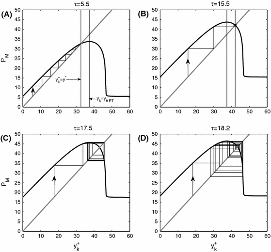

  

  The Poincaré map $P_M$ and stability of fixed point $y^*$. The parameter values are fixed as follows: $r=1.5, K=100, \beta =0.3, \eta =0.75, \omega =0.3, \hbox {ET}=50, \delta =0.8, \tau =15.5$ and $\theta =0.3$. a $\tau =5.5$, b $\tau =15.5$, c $\tau =17.5$, $\mathrm{d}\tau =18.2$

• (ii) $P_M$ is continuously differentiable.

• (iii) $P_M$ is concave on $[0,y_{\theta \mathrm{ET}})$.

• (iv) A unique positive fixed point $\tilde{y}$ exists for $P_M$. In particular, if $\tau >0$ and $P_M(y_{\theta \mathrm{ET}})<y_{\theta \mathrm{ET}}$, then $\tilde{y}\in (0, y_{\theta \mathrm{ET}})$; if $\tau >0$ and $P_M(y_{\theta \mathrm{ET}})> y_{\theta \mathrm{ET}}$, then $\tilde{y}\in (y_{\theta \mathrm{ET}}, +\infty )$.

• (v) There is a horizontal asymptote $y=\tau$ for $P_M$ as $y_k^+\rightarrow +\infty$.

Proof

• (i) It follows from the vector field of system (2) without impulsive effects that the definition domain of $P_M$ is $[0,+\infty )$. For any $y_{k_1}^+, y_{k_2}^+\in [0, y_{\theta \mathrm{ET}}]$ with $y_{k_1}^+<y_{k_2}^+$, it is easy to see that $y((1-\theta )\mathrm{ET}, y_{k_1}^+)<y((1-\theta )\mathrm{ET}, y_{k_2}^+)$ according to the uniqueness of the solution of model (1), and consequently we have $P_M(y_{k_1}^+)<P_M(y_{k_1}^+)$. For $y_{k_i}^+\in [y_{\theta \mathrm{ET}},+\infty ), i=1,2$ with $y_{k_1}^+<y_{k_2}^+$, the orbits $\Psi (t,t_0,(1-\theta )\mathrm{ET}, y_{k_i}^+)$ will cross the line $L_3$ once before it hits the line $L_4$. Denote the vertical coordinates of two orbits $\Psi (t,t_0,(1-\theta )$ET, $y_{k_i}^+)$ intersecting with the line $L_3$ are as $y_{q_i}^+, i=1,2$, and note that the order of the two new positions $y_{q_1}^+, y_{q_2}^+$ are inverted (i.e., $y_{q_1}^+> y_{q_2}^+$). The similar process of the previous case yields

  $$\begin{aligned} P_M(y_{k_1}^+)=P_M(y_{q_1}^+)>P_M(y_{q_2}^+)=P_M(y_{k_2}^+). \end{aligned}$$

  Therefore, $P_M$ is increasing on $[0, y_{\theta \mathrm{ET}}]$ and decreasing on $[y_{\theta }$ ET,$+\infty )$. Meanwhile, the range of $P_M$ takes the form $[\tau , y((1-\theta )$ET,$y_{\theta \mathrm{ET}})+\tau ].$

• (ii) It follows from model (1) that both functions $P(x,y)$ and $Q(x,y)$ are continuous and differentiable in the first quadrant. Therefore, the continuity and differentiability of $P_M$ can be confirmed by using the theorem of continuity and differentiability of the solution of an ordinary differential equation with respect to its initial condition, i.e., the theorem of Cauchy and Lipschitz with parameters. Furthermore, since $P(x,y)$ and $Q(x,y)$ are $C^{\infty }$, and thus, the theorem of Cauchy and Lipschitz with parameters implies that the Poincaré map $P_M$ is also $C^{\infty }$.

• (iii) It follows from (9) that

  $$\begin{aligned}&\displaystyle \frac{\partial g}{\partial y} = \displaystyle \frac{rx\Big (1-\frac{x}{K}\Big )\Big (\frac{\eta \beta x}{1+\omega x}-\delta \Big )}{\Big [rx\Big (1-\frac{x}{K}\Big )-\frac{\beta xy}{1+\omega x}\Big ]^2},\\&\displaystyle \frac{\partial ^2 g}{\partial y^2} = \displaystyle \frac{2rx\Big (1-\frac{x}{K}\Big )\Big (\frac{\eta \beta x}{1+\omega x}-\delta \Big ) \frac{\beta x}{1+\omega x}}{\Big [rx\Big (1-\frac{x}{K}\Big )-\frac{\beta xy}{1+\omega x}\Big ]^3}. \end{aligned}$$

  Since $x\le \mathrm{ET}$, we obtain $({\eta \beta x})/({1+\omega x})-\delta <0$ while $rx\Big (1-{x}/{K}\Big )-({\beta xy})/({1+\omega x})>0$ for $y<y_{\theta \mathrm{ET}}$ and $rx(1-{x}/{K})-({\beta xy})/({1+\omega x})<0$ for $y>y_{\theta \mathrm{ET}}$. Those indicate that $({\partial g})/({\partial y})<0$ and $({\partial ^2 g})/({\partial y^2})<0$ for all $y<y_{\theta \mathrm{ET}}$. According to the theorem of Cauchy and Lipschitz with parameters on the scalar differential equation, we have

  $$\begin{aligned}&\frac{\partial y(x,S)}{\partial S} \nonumber \\&\quad = \exp \left( \int _{(1-\theta )\mathrm{ET}}^{x}\frac{\partial }{\partial y}\left( \frac{Q(z,y(z,S))}{P(z,y(z,S))}\right) \mathrm{d}z\right) \nonumber \\&\quad >0 \end{aligned}$$

  (14)

  and

  $$\begin{aligned} \frac{\partial ^2y(x,S)}{\partial S^2}= & {} \frac{\partial y(x,S)}{\partial S}\int _{(1-\theta )\mathrm{ET}}^{x}\frac{\partial ^2}{\partial y^2} \nonumber \\&\left( \frac{Q(z,y(z,S))}{P(z,y(z,S))}\right) \frac{\partial y(z,S)}{\partial S}\mathrm{d}z. \end{aligned}$$

  (15)

  It is easy to see that $({\partial ^2y(x,S)})/({\partial S^2})<0$, and consequently we have $P_M$ is monotonic increasing and concave for $y<y_{\theta \mathrm{ET}}$, as shown in Fig. 1.

• (iv) Since $P_M$ is decreasing on $[y_{\theta \mathrm{ET}}, +\infty )$, there exists a $\overline{y}\in [y_{\theta \mathrm{ET}},+\infty )$ such that $P_M(\overline{y})<\overline{y}$. Moreover, it is easy to see that $P_M(0)=\tau \ge 0$, which indicates that there is $\tilde{y}\in [0,\overline{y})$ such that $P_M(\tilde{y})=\tilde{y}$, i.e., there exists a fixed point on $[0,+\infty )$ for $P_M$. Note that if $\tau >0$, then $\tilde{y}\in (0,\overline{y})$ must hold true. If $\tau >0$ and $P_M(y_{\theta \mathrm{ET}})<y_{\theta \mathrm{ET}}$, then the fixed point $\tilde{y}\in (0, y_{\theta \mathrm{ET}})$. On the one hand, since $P_M$ is decreasing on $[y_{\theta \mathrm{ET}}, +\infty )$, we have $P_M(y_k^+)<P_M(y_{\theta \mathrm{ET}})<y_{\theta \mathrm{ET}}$ for $y_k^+\in [y_{\theta \mathrm{ET}}, +\infty )$, which indicates no fixed point exists for $P_M$ on $[y_{\theta \mathrm{ET}}, +\infty )$. On the other hand, $P_M$ is concave on $(0, y_{\theta \mathrm{ET}})$, so a unique fixed point exists for $P_M$ on $(0, y_{\theta \mathrm{ET}})$. If $\tau >0$ and $P_M(y_{\theta \mathrm{ET}})>y_{\theta \mathrm{ET}}$, on the one hand, no fixed point exists for $P_M$ on $(0, y_{\theta \mathrm{ET}}]$ due to the concavity and $P_M(0)>0$; on the other hand, since $P_M$ is decreasing on $(y_{\theta \mathrm{ET}}, +\infty )$, there is a unique fixed point for $P_M$ on $(y_{\theta \mathrm{ET}}, +\infty )$.

• (v) Denote the closure of the ${\varOmega }_1$ as

  $$\begin{aligned} \bar{{\varOmega }}_1= & {} \left\{ (x,y): y\le \frac{r}{\beta }\left[1-\frac{x}{K}\right] \right. \nonumber \\&\left. (1+\omega x), x\ge 0\, \mathrm {and}\, y\ge 0 \right\} . \end{aligned}$$

We claim that the set $\bar{{\varOmega }}_1$ is an invariant set of system (1) if model (1) does not exist interior equilibrium $E^*$. In fact, let

$$\begin{aligned} L=y-\frac{r}{\beta }\left[1-\frac{x}{K}\right](1+\omega x) \end{aligned}$$

and $\bar{{\varOmega }}_1$ is an invariant set of system (1) if the vector field is flowing into of the boundary $\bar{{\varOmega }}_1$. This is true if

where stands for the scalar product of two vectors, so it is equivalent to

Moreover, for any $(x,y)$ belongs to the interior of $\bar{{\varOmega }}_1$ (i.e., ${\varOmega }_1$), we have $({\hbox {d}x(t)})/({\hbox {d}t})>0$ and $({\hbox {d}y(t)})/({\hbox {d}t})<0$. Therefore, we claim that $\mathcal {P}(+\infty )=0$ with $((1-\theta )\hbox {ET}, +\infty )\in {\mathcal {N}}$, i.e., $P_M(+\infty )=\tau$. Otherwise, there exists a positive $y_*$ such that $\mathcal {P}(+\infty )=y^*$ with $P_*=(\hbox {ET}, y_*)\in {\mathcal {M}}$. Taking any point $P_1=(\hbox {ET}, y_1)$ with $0<y_1<y_*$, then according to the invariance of the set $\bar{{\varOmega }}_1$ and the uniqueness of solution of model (1) the backward orbit initiating $P_1$ will reach a point $P_0^+=((1-\theta )\hbox {ET}, y_0^+)\in {\mathcal {N}}$ with $y_0^+>+\infty$, which is a contradiction. Thus, we have $\mathcal {P}(+\infty )=0$ and $P_M(+\infty )=\tau$, and consequently, there does exist a horizontal asymptote $y=\tau$ for $P_M$, as shown in Fig. 1. This completes the proof. $\square$

It is worth mentioning that the unique fixed point of Poincaré map $P_M$ corresponds to an order-1 periodic solution or order-1 limit cycle of system (2), which we address in more detail in the following subsection.

4.3 Global stability of boundary order-1 limit cycle for $\tau =0$

Letting $\tau =0$ and considering the following subsystem

$$\begin{aligned} \left\{ \begin{array}{l} \begin{array}{l} \displaystyle \frac{\hbox {d}x(t)}{\hbox {d}t}= rx(t)\left[1-\frac{x(t)}{K}\right] \end{array}\quad x<\hbox {ET},\\ \begin{array}{l} x(t^+)= (1-\theta )x(t),\\ \end{array}\quad x=\hbox {ET}.\\ \end{array}\right. \end{aligned}$$

(16)

Solving the first equation with initial condition $x(0^+)=(1-\theta )\hbox {ET}$, one yields

$$\begin{aligned} x(t)=\frac{K}{1+\left[\frac{K}{(1-\theta )\hbox {ET}}-1\right]\exp (-rt)}. \end{aligned}$$

Assume that $x(t)$ reaches the line $L_4$ at time $T$, then we have

$$\begin{aligned} \hbox {ET}=\frac{K}{1+\left[\frac{K}{(1-\theta )\hbox {ET}}-1\right]\exp (-rT)}. \end{aligned}$$

Further, solving the above equation with respect to $T$, one has

$$\begin{aligned} T=\frac{1}{r}\ln \left[\frac{K-\hbox {ET}(1-\theta )}{(1-\theta )(K-\hbox {ET})}\right]. \end{aligned}$$

Therefore, model (16) has a periodic solution, denoted by $x^T(t)$ and

$$\begin{aligned} x^T(t)=\frac{K}{1+\left[\frac{K}{(1-\theta )\hbox {ET}}-1\right]\exp (-rt)} \end{aligned}$$

with period $T$, which means that for model (2) there exists a boundary order-1 limit cycle $(x^T(t),0)$, and we have following main results.

Theorem 2

For case $(C_1)$, if $\tau =0$, then the boundary order-1 limit cycle $(x^T(t), 0)$ is globally asymptotically stable.

Proof

We first prove that the boundary order-1 limit cycle $(x^T(t),0)$ is locally stable. To do this, by using Lemma 1, we denote $\phi (x,y)=x-\hbox {ET},\, a(x,y)=-\theta x$ and $b(x,y)=\tau$. By simple calculations, we have

$$\begin{aligned}&\frac{\partial P}{\partial x} = \frac{r(K-2x)}{K}-\frac{\beta y}{(1+\omega x)^2}, \frac{\partial Q}{\partial y}=\frac{\eta \beta x}{1+\omega x}-\delta ,\\&\frac{\partial a}{\partial x} = -\theta , \frac{\partial a}{\partial y}=\frac{\partial b}{\partial x}=\frac{\partial b}{\partial y}=0,\\&\frac{\partial \phi }{\partial x} = 1, \frac{\partial \phi }{\partial y}=0 \end{aligned}$$

and $\triangle _1={P_+((1-\theta )\hbox {ET}, 0)}/{P(\hbox {ET}, 0)}={((1-\theta )}$ ${(K-(1-\theta )\hbox {ET}))}/({K-\hbox {ET}})$. Thus,

$$\begin{aligned} \displaystyle \int _0^T\left( \frac{\partial P}{\partial x} +\frac{\partial Q}{\partial y}\right) \hbox {d}t= & {} \displaystyle \int _0^T\left( \frac{r(K-2x^T(t))}{K} \right. \nonumber \\&\left. +\frac{\eta \beta x^T(t)}{1+\omega x^T(t)}-\delta \right) \hbox {d}t \\\doteq & {} I_1+I_2+I_3, \end{aligned}$$

where the first term can be calculated as follows

$$\begin{aligned} I_1=\ln \left[\frac{K-ET}{(1-\theta )(K-ET(1-\theta ))}\right], \end{aligned}$$

the second term can be calculated as

and the third term is as follows

$$\begin{aligned} I_3=-\delta T=-\frac{\delta }{r}\ln \left[\frac{K-\hbox {ET}(1-\theta )}{(1-\theta )(K-\hbox {ET})}\right]. \end{aligned}$$

Hence, we have

$$\begin{aligned} |\mu _2|= & {} \frac{(1-\theta )(K-(1-\theta )\hbox {ET})}{K-\hbox {ET}}\exp \left( I_1+I_2+I_3\right) \\= & {} \exp (A_\mathrm{ET}) \end{aligned}$$

with

$$\begin{aligned} A_{ET}=I_2+I_3. \end{aligned}$$

(17)

Therefore, if $|\mu _2|<1$ (i.e., $A_\mathrm{ET}<0$), then the boundary order-1 limit cycle is orbitally asymptotically stable and enjoys the property of asymptotic phase.

Now, we claim $|\mu _2|<1$ when $R_0\le 1$. In fact, it follows from $[1+\omega \hbox {ET}(1-\theta )][K-\hbox {ET}]-[1+\omega \hbox {ET}][K-\hbox {ET}(1-\theta )]=-\theta \hbox {ET}(1+\omega K)<0$ that we have $I_2>0$, and it is easy to see that $I_3<0$ always holds true. This indicates that the sign of $A_\mathrm{ET}$ could vary which depends on the different parameter sets. It follows from $R_0\le 1$ (i.e., $\eta \beta -\delta \omega \le \delta /K$) that we have $\eta \beta K\le \delta (1+\omega K)$, and consequently, we have

Finally, we show that the boundary order-1 limit cycle $(x^T(t), 0)$ is globally attractive. To do this, we assume, without loss of generality, that the impulsive point series $y_k^+$ of any solution starting from the phase set ${\mathcal {N}}$ satisfies $y_k^+\in [0, y_{\theta \mathrm{ET}}]$ for all $k\ge 0$. Since $R_0\le 1$ and $\hbox {ET}<K$, we have $({\hbox {d}y})/({\hbox {d}t})<0$ for $x\le \hbox {ET}$. Thus, we conclude that $y_k^+$ is a strictly decreasing sequence with $\lim \nolimits _{k\rightarrow \infty }y_k^+=y^*$. Moreover, $y^*=0$ must hold; otherwise, it contradicts with $({\hbox {d}y})/({\hbox {d}t})<0$ for $x\le \hbox {ET}$. Therefore, the boundary order-1 limit cycle $(x^T(t), 0)$ is globally attractive. This completes the proof.$\square$

The stability of the boundary order-1 limit cycle has been numerically shown in Fig. 2a–c for case $(C_1)$, from which we can see that the natural enemy population decreases and dies out eventually if the releasing constant $\tau =0$, while the pest population will oscillate periodically with a relative high frequency.

Fig. 2

Stability of the boundary order-1 limit cycles for cases $(C_1)$ and $(C_2)$. The parameter values are fixed as follows: a–c $r=1.5, K=100, \beta =0.3, \eta =0.75, \omega =0.3, \hbox {ET}=50, \delta =0.8, \theta =0.3, \tau =0$ for case $(C_1)$; d–i $r=1, K=52, \beta =0.19, \eta =0.45, \omega =0.19, \hbox {ET}=35, \delta =0.56$ in d–f with $A_\mathrm{ET}<0$ and $\delta =0.36$ in g–i with $A_\mathrm{ET}>0$, $\tau =0$ for case $(C_2)$

4.4 Existence and stability of order-$k$ periodic solutions for $\tau >0$

Before we address the existence of order-$k$ periodic solution, we initially provide a generalized result for the stability of the order-1 limit cycle $(\xi (t), \eta (t))$. To do this, without loss of generality, we assume that the period of the order-1 periodic solution is $T$, and we have

$$\begin{aligned} (\xi (T), \eta (T))= & {} (\hbox {ET}, y^*), \quad (\xi (T^+), \eta (T^+)) \\= & {} ((1-\theta )\hbox {ET}, y^*+\tau ). \end{aligned}$$

Thus, $\triangle _1=\frac{P_+((1-\theta )\hbox {ET}, y^*+\tau )}{P(\hbox {ET}, y^*)}$ and

$$\begin{aligned}&\displaystyle \int _0^T\left( \frac{\partial P}{\partial x}+\frac{\partial Q}{\partial y}\right) \hbox {d}t = \displaystyle \int _0^T\left( \frac{r(K-2\xi (t))}{K} \right. \\&\quad \left. -\frac{\beta \eta (t)}{(1+\omega \xi (t))^2}+\frac{\eta \beta \xi (t)}{1+\omega \xi (t)}-\delta \right) \hbox {d}t\\&\quad \doteq \displaystyle \int _0^TG(t)\hbox {d}t. \end{aligned}$$

Therefore, according to Lemma 1, we have the following generalized result.

Theorem 3

For case $(C_1)$, the order-1 limit cycle $(\xi (t), \eta (t))$ of model (2) is locally stable if $|\triangle _1|\exp \left( \int _0^TG(t)\mathrm{d}t\right) <1$.

For case $(C_1)$, there is an infinite sequence $\{y_n^+\}$ for any $y_0^+\in [0, +\infty )$, where $y_n^+=P_M^n(y_0^+)$. In the following, we examine the convergence of $\{y_n^+\}$, which indeed refers to the stability of the order-$k\,(k\ge 1)$ periodic solutions or limit cycles of system (2).

Theorem 4

If $P_M(y_{\theta \mathrm{ET}})< y_{\theta \mathrm{ET}}$, then the Poincaré map $P_M$ has a unique fixed point $y^*$ (i.e., model (2) exists a unique order-1 limit cycle), which is globally asymptotically stable.

Proof

To prove Theorem 4, we only need to show that the unique fixed point of the Poincaré map $P_M$ is globally asymptotically stable. It follows from property (iv) of the Poincaré map $P_M$ shown in Theorem 1 that there exists a unique $y^* \in (0, y_{\theta \mathrm{ET}})$ such that $P_M(y^*)=y^*$ if $P_M(y_{\theta \mathrm{ET}})< y_{\theta \mathrm{ET}}$.

For any $y_0^+\in [0, y^*)$, according to the concavity of the $P_M$ on $[0, y_{\theta \mathrm{ET}})$, we have $y^*>P_M(y_0^+)>y_0^+$, which indicates that $P_M^n(y_0^+)$ is monotonically increasing as $n$ increases and $\lim _{n\rightarrow +\infty }P_M^n(y_0^+)=y^*$, as shown in Fig. 1a.

For any $y_0^+>y^*$, we consider the following two cases: (a) for all $n$, we have $P_M^n(y_0^+)>y^*$. It follows from $P_M(y_0^+)<y_0^+$ that the series of $P_M^n(y_0^+)$ is monotonically decreasing as $n$ increases and $\lim _{n\rightarrow +\infty }P_M^n(y_0^+)=y^*$. (b) $P_M^n(y_0^+)>y^*$ does not hold true for all $n$, and according to the property (v) of the $P_M$, we conclude that there exists a smallest positive integer $n_1$ such that $P_M^{n_1}(y_0^+)<y^*$. Therefore, by employing the same method as those in case (a), we have that $P_M^{n_1+j}(y_0^+)$ is monotonically increasing as $j$ increases and $\lim _{j\rightarrow +\infty }P_M^{n_1+j}(y_0^+)=y^*$. Thus, the results shown in Theorem 4 are true, and this completes the proof. $\square$

Remark 1

By using same methods as those in Theorem 4, we can prove that if $P_M(y_{\theta \mathrm{ET}})= y_{\theta \mathrm{ET}}$, then the Poincaré map $P_M$ has a unique fixed point $y_{\theta \mathrm{ET}}$ (i.e., model (2) exists a unique order-1 limit cycle), which is globally asymptotically stable.

If $P_M(y_{\theta \mathrm{ET}})>y_{\theta \mathrm{ET}}$, then the dynamics of the Poincaré map $P_M$ and model (2) could be very complex, as shown in Fig. 1. Therefore, for the existence and stability of order-1 or order-2 limit cycles, we first provide some sufficient or sufficient and necessary conditions, and then, we address the complex dynamics.

Theorem 5

If $P_M(y_{\theta \mathrm{ET}})>y_{\theta \mathrm{ET}}$ and $P_M^2(y_{\theta \mathrm{ET}})\ge y_{\theta \mathrm{ET}}$, then the Poincaré map $P_M$ has a stable fixed point or a stable two-point cycle. Consequently, there is a stable order-1 or order-2 limit cycle for system (2), as shown in Fig. 1b, c.

Proof

We claim that for $((1-\theta )\hbox {ET}, y_0^+)\in {\mathcal {N}}$ with $y_0^+\in [0,+\infty )$, there is an integer $p$ such that $y_p^+=P_M^p(y_0^+)\in [y_{\theta \mathrm{ET}}, P_M(y_{\theta \mathrm{ET}})]$. In fact, for $y_0^+$ $\in [0,y_{\theta \mathrm{ET}}]$, according to the Theorem 1, we conclude that there is no fixed point for $P_M$ on interval $[0,y_{\theta \mathrm{ET}}]$ and $P_M$ is monotonically increasing on $[0, y_{\theta \mathrm{ET}}]$. Therefore, there is an integer $p$ such that $y_{p-1}^+<y_{\theta \mathrm{ET}}$ and $y_p^+\ge y_{\theta \mathrm{ET}}$. It follows that $y_p^+=P_M(y_{p-1}^+)\le P_M(y_{\theta \mathrm{ET}})$, which indicates that $y_p^+\in [y_{\theta \mathrm{ET}},P_M(y_{\theta \mathrm{ET}})]$. For $y_0^+\in (y_{\theta \mathrm{ET}}, +\infty )$, since $P_M$ is monotonically decreasing on $(y_{\theta \mathrm{ET}}, +\infty ),\, y_1^+=P_M(y_0^+)\le P_M(y_{\theta \mathrm{ET}})$ and further there is an integer $p\ge 1$ such that $y_p^+\in [y_{\theta \mathrm{ET}}, P_M(y_{\theta \mathrm{ET}})]$.

It follows from $P_M$ is monotonically decreasing on $[y_{\theta \mathrm{ET}}, P_M(y_{\theta \mathrm{ET}})]$ and $P_M^2$ is monotonically increasing on $[y_{\theta \mathrm{ET}}, P_M(y_{\theta \mathrm{ET}})]$ that

$$\begin{aligned}&P_M([y_{\theta \mathrm{ET}}, P_M(y_{\theta \mathrm{ET}})])\\&\quad =[P_M^2(y_{\theta \mathrm{ET}}), P_M(y_{\theta \mathrm{ET}})] \subset [y_{\theta \mathrm{ET}}, P_M(y_{\theta \mathrm{ET}})]. \end{aligned}$$

Based on above relations, for any $y_0^+\in [y_{\theta \mathrm{ET}}, P_M(y_{\theta \mathrm{ET}})]$ without loss of generality, we assume that $y_1^+=P_M(y_0^+)\ne y_0^+$ and $y_2^+=P_M^2(y_0^+)\ne y_0^+$ with $y_n^+=P_M^n(y_0^+)$, i.e., the solution of model (2) initiating from $((1-\theta )\hbox {ET}, y_0^+)$ is neither an order-1 periodic solution nor an order-2 periodic solution. Thus, we only need to consider the following four possible cases:

• (i) $P_M(y_{\theta \mathrm{ET}})\ge y_1^++>y_0^+>y_2^+\ge y_{\theta \mathrm{ET}}$. In this case, we have $y_3^+=P_M(y_2^+)>P_M(y_0^+)=y_1^+$ and further $y_4^+=P_M(y_3^+)<P_M(y_1^+)=y_2^+$, so $y_3^+>y_1^+>y_0^+>y_2^+>y_4^+$. By induction, we obtain

  

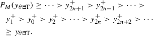  (18)

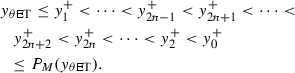
• (ii) $P_M(y_{\theta \mathrm{ET}})\ge y_1^+>y_2^+>y_0^+\ge y_{\theta \mathrm{ET}}$. In this scenario, we obtain that $P_M(y_1^+)=y_2^+<y_3^+=P_M(y_2^+)<P_M(y_0^+)=y_1^+$ and $P_M(y_2^+)=y_3^+>y_4^+=P_M(y_3^+)>P_M(y_1^+)=y_2^+$, which results in $y_1^+>y_3^+>y_4^+>y_2^+>y_0^+$. Again, by induction, we derive

  

  (19)

• (iii) $y_{\theta \mathrm{ET}}\le y_1<y_2<y_0\le P_M(y_{\theta \mathrm{ET}})$. The similar process to (ii) yields

  

  (20)

• (iv) $y_{\theta \mathrm{ET}}\le y_1^+<y_0^+<y_2^+\le P_M(y_{\theta \mathrm{ET}})$. Performing the similar discussion to (1) gives

  

  (21)

For cases (ii) and (iii), there either exists a unique $y^*$ with $y^*\in [y_{\theta \mathrm{ET}},P_M(y_{\theta \mathrm{ET}})]$ such that $\lim _{n\rightarrow \infty }y_{2n+1}=\lim _{n\rightarrow \infty }y_{2n}=y^*$ or exists two distinct values $y_1^*, y_2^*$ with $y_1^*, y_2^*\in [y_{\theta \mathrm{ET}},P_M(y_{\theta \mathrm{ET}})]$ and $y_1^*\ne y_2^*$ such that $\lim _{n\rightarrow \infty }y_{2n+1}=y_1^*$ and $\lim _{n\rightarrow \infty }y_{2n}=y_2^*$. While for cases (i) and (iv), only the late case can be true. All those confirm that the results shown in Theorem 5 hold true. $\square$

Although Theorem 5 provides a useful sufficient condition for existence and stability of an order-1 or order-2 limit cycle of model (2) when $P_M(y_{\theta \mathrm{ET}})>y_{\theta \mathrm{ET}}$, this can not determine whether the order-1 limit cycle is globally stable or not. So we present the following main results with respect to the global stability of order-1 limit cycle [19–21].

Theorem 6

If $P_M(y_{\theta \mathrm{ET}})>y_{\theta \mathrm{ET}}$, then the sufficient and necessary condition for the global stability of the order-1 limit cycle of model (2) is $P_M^2(y^+)>y^+$ for all $y^+\in [y_{\theta \mathrm{ET}}, y^*)$, as shown in Fig. 1b.

Proof

If $P_M(y_{\theta \mathrm{ET}})>y_{\theta \mathrm{ET}}$, then according to the Theorem 1, we conclude that there exists a unique fixed point $y^*$ of the Poincaré map such that it satisfies: (i) $P_M(y^+)>y^+$ for $y^+\in [0, y^*)$ and $P_M(y^+)<y^+$ for $y^+\in (y^*, +\infty )$; (ii) $P_M(y^+)$ reaches its maximal value at $y_{\theta \mathrm{ET}}$ with $y_{\theta \mathrm{ET}}\in (0, y^*)$; moreover, $P_M(y^+)$ is monotonically decreasing for $y^+\in (y_{\theta \mathrm{ET}}, y^*)$, as shown in Fig. 1b, c.

Sufficient condition In order to prove the sufficient condition of Theorem 6, based on above discussion, we consider the following three intervals: (a) $y^+\in [y_{\theta \mathrm{ET}}, y^*)$; (b) $y^+\in [0, y_{\theta \mathrm{ET}})$; and (c) $y^+\in (y^*, +\infty )$.

For case (a), it follows from $y_{\theta \mathrm{ET}}\le y^+<y^*$ and the monotonicity of $P_M$ in this interval that we have $P_M(y_{\theta \mathrm{ET}})\ge P_M(y^+)>y^*$, and further from $P_M^2(y^+)>y^+$ for all $y^+\in [y_{\theta \mathrm{ET}}, y^*]$ that $y^+<P_M^2(y^+)<y^*$. By induction, we conclude that $P_M^{2(j-1)}<P_M^{2j}<y^*$ for all $j\ge 1$, which indicates that $P_M^{2j}(y^+)$ is monotonically increasing with $\lim _{j\rightarrow +\infty }P_M^{2j}(y^+)=y^*$ and the monotonicity of $P_M^{2j-1}(y^+)$ follows as well.

For case (b), it is easy to know that $P_M$ is monotonically increasing, and then, there exists a positive integer $p$ such that either $P_M^p(y^+)\in [y_{\theta \mathrm{ET}}, y^*)$ or $P_M^p(y^+)>y^*$. It follows from case (a) that the former case $P_M^p(y^+)\in [y_{\theta \mathrm{ET}}, y^*)$ indicates that $\lim \nolimits _{j\rightarrow +\infty }P_M^{p+2j}(y^+)=y^*$ monotonically. The late case $P_M^p(y^+)>y^*$ implies that there exists a $\bar{y}^+\in (y_{\theta \mathrm{ET}}, y^*)$ such that $P_M^p(y^+)=P_M(\bar{y}^+)$. Again it follows from case (a) that we have $\lim \limits _{j\rightarrow +\infty }P_M^{p+2j}(y^+)=y^*$ monotonically.

For case (c), if for all $j$ we have $P_M^j(y^+)>y^*$, then it follows from $P_M(y^+)<y^+$ that $P_M^{j}(y^+)$ is monotonically decreasing with $\lim \limits _{j\rightarrow +\infty }P_M^{j}(y^+)=y^*$; if there exists a positive integer $p$ such that $P_M^{p}(y^+)\in (0, y_{\theta \mathrm{ET}}) (\mathrm {or} \ [y_{\theta \mathrm{ET}}, y^*))$, then according to cases (a) and (b) we see that the result is true.

Necessary condition Assume that $y^*$ is globally stable and we prove $P_M^2(y^+)>y^+$ for all $y^+\in [y_{\theta \mathrm{ET}}, y^*)$. Otherwise, there exists at least a $\hat{y}^+\in [y_{\theta \mathrm{ET}}, y^*)$ such that $P_M^2(\hat{y}^+)<\hat{y}^+$. It follows from the local stability of $y^*$ that there exists $\check{y}^+\in (y^*-\epsilon , y^*+\epsilon )$ (where $\epsilon$ is small enough) such that $P_M^2(\check{y}^+)>\check{y}^+$. Therefore, it follows from Theorem 1 that the Poincaré map is continuous and there exists a $y^{**}$ which lies between $\hat{y}^+$ and $\check{y}^+$ such that $P_M^2(y^{**})=y^{**}$, i.e., the solution of model (2) initiating from $((1-\theta )\hbox {ET}, y^{**})$ is an order-2 periodic solution. This contradicts with the global stability of $y^*$, i.e., the global stability of the order-1 limit cycle. $\square$

Theorem 7

If $P_M(y_{\theta \mathrm{ET}})>y_{\theta \mathrm{ET}}, P_M^2(y_{\theta \mathrm{ET}})<y_{c}^+$, where $y_{c}^+=\min \{y^+: P_M(y^+)=y_{\theta \mathrm{ET}}\}$, then there exists a nontrivial order-3 periodic solution for model (2), and so nontrivial order-$k\, (k\ge 3)$ periodic solution exists for system (2).

Proof

Since $P_M(y_{\theta \mathrm{ET}})>y_{\theta \mathrm{ET}}$, there is a unique fixed point $y^*$ of the Poincaré map $P_M$ satisfying $y^*\in (y_{\theta \mathrm{ET}}, P_M(y_{\theta \mathrm{ET}}))$.

Let $H(y)=P_M^3(y)-y$, and then, $H(y)$ is continuous on $[0,+\infty )$. It follows from

$$\begin{aligned} P_M^3(y_{c}^+)= & {} P_M^2(y_{\theta \mathrm{ET}})<y_{c}^+ \Rightarrow H(y_{c}^+)<0 \, \text{ and } \nonumber \\ P_M^3(0)= & {} P_M^2(\tau )>0 \Rightarrow H(0)>0 \end{aligned}$$

that there is a number $\tilde{y}^+\in (0,y_{c}^+)$ such that $P_M^3(\tilde{y}^+)=\tilde{y}^+$. It follows from $y_{c}^+<y_{\theta \mathrm{ET}},\, y^*>y_{\theta \mathrm{ET}}$ and the uniqueness of $y^*$ that model (2) exists a nontrivial order-3 periodic solution initiating from $((1-\theta )\hbox {ET},\tilde{y}^+)$. Further, it follows from Sarkovskii’s theorem [15] that any order-$k$ periodic solution exists for system (2). This completes the proof.

As an example, we fixed all parameter values as those shown in Fig. 3, from which we can see that the parameter set satisfies case $(C_1)$, i.e., model (2) does not exist interior equilibrium $E^*$. The bifurcation diagrams with respect to $\theta$ ($0.1\le \theta \le 0.95$) show that the dynamic behavior of model (2) is very complex. In particular, the order-3 periodic solution exists for a wide range of $\theta$, as shown in Fig. 3a, b), which further confirms that the results shown in Theorem 7 are true. Comparing with both bifurcation diagrams with different threshold value ET, we conclude that varying ET could dramatically change the dynamics of model (2), and it is interesting to note that the period doubling and period halving bifurcations occur as ET$\,=\,50$, as shown in Fig. 3c, d. The islands in the middle of Fig. 3c, d indicate that the densities of both pest and natural enemy populations reveal complex patterns when the instantaneous killing rate $\theta$ lies in the interval around (0.6, 0.7).

Fig. 3

Bifurcation diagrams with respect to $\theta$ under which the model does not exist interior equilibrium. The parameter values are fixed as follows: a, b $r=1.5, K=100, \beta =0.3, \eta =0.75, \omega =0.3, \hbox {ET}=30, \delta =0.8, \tau =15.5$; c, d $r=1.5, K=100, \beta =0.3, \eta =0.75, \omega =0.3, \hbox {ET}=50, \delta =0.8, \tau =15.5$

In the following, we provide a sufficient condition for the existence and global stability of an order-1 limit cycle of model (2) based on all parameters rather than using the Poincaré map $P_M$.

Theorem 8

There exists a threshold $\omega _c$ which depends on the other parameters of model (2) such that the unique order-1 limit cycle of model (2) is globally stable for $\omega >\omega _c$ and fixed all other parameters.

Proof

Note that we focus on the nonexistence of the interior equilibrium in this section, i.e., $R_0=({K[\eta \beta -\delta \omega ]})/{\delta }\le 1$. Therefore, if we consider the $R_0$ as a function of $\omega$, then there exists a threshold value $\omega _c=({\eta \beta })/{\delta }$ such that $R_0<1$ and $\eta \beta -\delta \omega <0$ for all $\omega >\omega _c$. In the interior of ${\varOmega }$, we have $P(x,y)>0$ and $Q(x,y)<0$ due to the nonexistence of equilibrium. Thus, we have following inequality within ${\varOmega }$

$$\begin{aligned} \displaystyle \frac{Q(x,y)}{P(x,y)}<\displaystyle \frac{Q(x,y)}{rx\left(1-\displaystyle \frac{x}{K}\right)}. \end{aligned}$$

(22)

Considering the following Cauchy problem

$$\begin{aligned} \left\{ \begin{array}{l} \displaystyle \frac{\mathrm {d}Y}{\mathrm {d}x}=\displaystyle \frac{\displaystyle \frac{\eta \beta xY}{1+\omega x}-\delta Y}{rx(1-\displaystyle \frac{x}{K})}\dot{=}G(x,Y),\\ Y((1-\theta )\hbox {ET})=y_{\theta \mathrm{ET}} \end{array} \right. \end{aligned}$$

(23)

and solving above equation for $x\in [(1-\theta ) \hbox {ET}, \hbox {ET}]$, one yields

(24)

which indicates that (denote $Y_\mathrm{ET}=Y(\hbox {ET})$ and $\theta _1=1-\theta$)

$$\begin{aligned} Y_\mathrm{ET}= & {} y_{\theta \mathrm{ET}}\left(\frac{\theta _1}{1}\right)^{\displaystyle \frac{\delta }{r}}\left(\frac{K-\hbox {ET}}{K-\theta _1\hbox {ET}}\right)^{\displaystyle \frac{\delta \omega K-\eta \beta K+\delta }{r(1+\omega K)}} \nonumber \\&\left(\frac{1+\omega \hbox {ET}}{1+\omega \theta _1\hbox {ET}}\right)^{\displaystyle \frac{\eta \beta K }{r(1+\omega K)}}. \end{aligned}$$

(25)

Furthermore, we have

$$\begin{aligned}&\lim _{\omega \rightarrow +\infty }\left(\displaystyle \frac{\theta _1}{1}\right)^{\displaystyle \frac{\delta }{r}}\left(\displaystyle \frac{K-\hbox {ET}}{K-\theta _1\hbox {ET}}\right)^{\displaystyle \frac{\delta \omega K-\eta \beta K+\delta }{r(1+\omega K)}} \\&\quad \left(\displaystyle \frac{1+\omega \hbox {ET}}{1+\omega \theta _1\hbox {ET}}\right)^{\displaystyle \frac{\eta \beta K }{r(1+\omega K)}} \\&\quad =\left(\displaystyle \frac{\theta _1(K-\hbox {ET})}{K-\theta _1\hbox {ET}}\right)^{\displaystyle \frac{\delta }{r}}<1 \end{aligned}$$

and $\lim \nolimits _{\omega \rightarrow +\infty }y_{\theta \mathrm{ET}}=+\infty$.

All those confirm that the difference $y_{\theta \mathrm{ET}}-Y_\mathrm{ET}$ satisfies

$$\begin{aligned}&\lim _{\omega \rightarrow +\infty }\left[y_{\theta \mathrm{ET}}-Y_\mathrm{ET}\right]=\left[1-\left(\frac{\theta _1(K-\hbox {ET})}{K-\theta _1\hbox {ET}}\right)^{\displaystyle \frac{\delta }{r}}\right] \nonumber \\&\quad \lim _{\omega \rightarrow +\infty }y_{\theta \mathrm{ET}}=+\infty . \end{aligned}$$

(26)

Moreover, it follows from the comparison theorem of scalar differential equation and the theorem of Cauchy and Lipschitz with parameters that

$$\begin{aligned} y_{\theta \mathrm{ET}}-y_\mathrm{ET}>y_{\theta \mathrm{ET}}-Y_\mathrm{ET} \end{aligned}$$

(27)

and $P_M(y_{\theta \mathrm{ET}})=y_\mathrm{ET}+\tau$. Thus, according to the limitation (26), we conclude that for the fixed parameter set there exists a threshold value $\omega _c=(\eta \beta )/\delta$ which depends on the parameters of model (2) such that $y_\mathrm{ET}+\tau <y_{\theta \mathrm{ET}}$, i.e., we have $P_M(y_{\theta \mathrm{ET}})<y_{\theta \mathrm{ET}}$ for all $\omega >\omega _c$. Further, it follows from Theorem 4 that the fixed point $y^*$ of the Poincaré map $P_M$ is globally stable, and consequently, the unique order-1 limit cycle of system (2) is globally stable. This completes the proof.

5 Complexity of definition domain of map $P_M$ for existence of $E^*$

For case $(C_2)$, we see that the equilibrium $E^*$ exists and it is an unstable node or focus. In this case, the definition domain of $P_M$ could be very complex, which depends on the relations among the positions of $(1-\theta )\hbox {ET}, \hbox {ET}$, $x_{{\varGamma }_1}$ and $x_{{\varGamma }_2}$. Thus, we investigate the dynamics of model (2) based on those relations.

We first assume that $(1-\theta )\hbox {ET}\le x_{{\varGamma }_1}$ and $\hbox {ET}< x_{{\varGamma }_2}$, then any solution starting from $((1-\theta )ET, y_0^+)$ with $y_0^+\ge 0$ will not only experience infinite many impulsive effects, but also the Poincaré map $P_M$ can be well defined which satisfies all properties listed in Theorem 1. Those indicate that the existence and stability of the order-$k$ periodic solutions can be discussed similarly. Thus, we only provide the different main result with regard to the boundary order-1 limit cycle in the following for this subcase.

Theorem 9

For case $(C_2)$, let $\tau =0$ and $(1-\theta )\mathrm{ET}\le x_{{\varGamma }_1}$ and $\mathrm{ET}< x_{{\varGamma }_2}$. The boundary order-1 limit cycle $(x^T(t), 0)$ is locally asymptotically stable provided $A_\mathrm{ET}<0$; the boundary order-1 limit cycle $(x^T(t), 0)$ is unstable and model rm (2) exists an interior order-1 periodic solution if $A_\mathrm{ET}>0$.

Proof

It follows from the proof of Theorem 2 that the boundary order-1 limit cycle $(x^T(t), 0)$ is locally asymptotically stable provided $A_\mathrm{ET}<0$, and it is unstable if $A_\mathrm{ET}>0$.

To show model (2) exists an interior order-1 periodic solution when $A_\mathrm{ET}>0$, we first show $P_M'(0)>1$. It follows from (11) and (14) that $({\partial y(x,S)})/({\partial S})>0$ and

(28)

This indicates that ${\mathcal {P}}'(0)=P_M'(0)>1$, and it follows from the properties of the Poincaré map $P_M$ shown in Theorem 1 that there must exist an intersection point between $P_M$ and identical map, as shown in Fig. 1. Thus, model (2) exists an interior order-1 periodic solution provided $A_\mathrm{ET}>0$. This completes the proof.

Taking the parameter values as those shown in Fig. 2 for case $(C_2)$, we can see that the boundary order-1 limit cycle is stable if $A_\mathrm{ET}<0$, and it becomes unstable once $A_\mathrm{ET}>0$ and an interior periodic solution appears in this case, as shown in Fig. 2g–i).

Now, we assume that $x_{{\varGamma }_1}<(1-\theta )\hbox {ET}<\hbox {ET}<x_{{\varGamma }_2}$, then the properties of the Poincaré map could be very complex, i.e., the definition domain of the map $P_M$ has a complex shape with discontinuity points. For convenience, we assume, without loss of generality, that the unstable equilibrium $E^*$ of model (1) is a focus, i.e., we have $\triangle =\left(({\mu C_1})/{\xi }\right)^2-4\mu C_2<0.$

If we fixed all parameter values as those shown in Fig. 4, then the Poincaré map $P_M$ has six discontinuity points at $y_k^+\approx 11.28, 14.50, 15.38, 15.74 16.15$ and $16.93$, as shown in Fig. 4a which are indicated as $D_i, i=1,2,\ldots 6$. Meanwhile, it has six fixed points with $y^*\approx 11.48, 13.42, 15.22, 15.81, 16.24$ and $17.00$, and consequently, model (2) exists six order-1 periodic solutions which lie in the interior of the unique limit cycle of model (1), as shown in Fig. 4b. Furthermore, numerical simulations indicate that only the order-1 periodic solution initiating from $((1-\theta )\hbox {ET}, 11.48)$ (i.e., the red one) is stable and all others are unstable. Therefore, compared with the main results for ODE model (1), the interesting question is how to determine the uniqueness of stable order-1 periodic solution or limit cycle of model (2), which could correspond to the uniqueness of the limit cycle of model (1).

Fig. 4

Discontinuity of Poincaré map and multiple fixed points with parameter set $r=1, K=52, \beta =0.19, \eta =0.45, \omega =0.19, \delta =0.36, \theta =0.42, \tau =5, ET=35$. In this case, the Poincaré map has six discontinuity points and six fixed points, and consequently, model (2) exists six order-1 limit cycles

We note that the number of discontinuity points of the Poincaré map $P_M$ for $x_{{\varGamma }_1}<(1-\theta )\hbox {ET}<\hbox {ET}<x_{{\varGamma }_2}$ depends on the number of intersection points of spiral orbits initiating from the line $L_3$ with the phase set ${\mathcal {N}}$ before it reaches at the line $L_4$, as shown in Fig. 4a. At each of these intersection points, the map $P_M$ is undefined and there exists a jump of the values of the map $P_M$, as shown in Fig. 5 for different $\theta$ and the bifurcation diagrams with respect to $\theta$ shown in Fig. 6. Figure 5 clearly shows the complexity of the definition domain of the Poincaré map $P_M$, at which we can see that the numbers of discontinuity points and fixed points depend on the parameter $\theta$, i.e., depend on the positions of reset line $L_3$.

Fig. 5

Complex shapes of the Poincaré map $P_M$ with different $\theta$. The other parameter values are fixed as: $r=1, K=52, \beta =0.19, \eta =0.45, \omega =0.19, \delta =0.36, \tau =5, \hbox {ET}=35$. a $\theta =0.8$, b $\theta =0.6$, c $\theta =0.52$, d $\theta =0.48$, e $\theta =0.3$, f $\theta =0.1$

Fig. 6

Bifurcation diagrams of discontinuity points and values of $y_0^+$ for $P_M$ with respect to parameter $\theta$ in a, and bifurcation diagram of number of fixed points and values of $y^*$ for $P_M$ with respect to parameter $\theta$ in b. The other parameter values are fixed as: $r=1, K=52, \beta =0.19, \eta =0.45, \omega =0.19, \delta =0.36, \tau =5, \hbox {ET}=35$

The bifurcation diagrams shown in Fig. 6 show how the numbers of discontinuity points and fixed points of map $P_M$ change as the parameter $\theta$ varies. There exists only one discontinuity point and does not has any fixed point once $\theta$ is small enough, for example, Fig. 5f. Two fixed points emerge as $\theta$ increases, and then, one more fixed point appears once the $\theta$ reaches another threshold value which corresponds to one discontinuity point. After that the numbers of discontinuity points and fixed points of map $P_M$ increase dramatically as $\theta$ increases. In particular, it is interesting to note that once the reset line $L_3$ coincides with the unstable equilibrium $E^*$, i.e., $(1-\theta )\hbox {ET}=x_e$, then the $E^*$ could be considered as a singularity point of model (2). If so the negative orbit spirals around $E^*$ and converges to it, there exists an infinite countable sequence of intersection points in the reset line $L_3$. This indicates that the Poincaré map $P_M$ for $x_{{\varGamma }_1}<(1-\theta )\hbox {ET}<\hbox {ET}<x_{{\varGamma }_2}$ with $(1-\theta )\hbox {ET}=x_e$ exists an infinite countable discontinuity points and the fixed points could also be infinite, as shown in Fig. 6. Consequently, model (2) may have infinite order-1 periodic solutions or limit cycles. Once the $\theta$ increases and exceeds another threshold value such as $\theta =0.8$ shown in Fig. 5a, then the map $P_M$ becomes continuous and exists a uniqueness fixed point.

Fig. 7

Bifurcation diagrams with respect to $\omega$ under which model (1) could exist a stable limit cycle ${\varGamma }_{(1)}$. The parameter values are fixed as follows: a, b $r=1.5, K=100, \beta =0.2, \eta =0.9, \hbox {ET}=40, \delta =0.2, \theta =0.9, \tau =4.5$; c, d $r=1.5, K=100, \beta =0.2, \eta =0.9, \hbox {ET}=80, \delta =0.2, \theta =0.9, \tau =4.5$

The period-incrementing or period-adding cascade of bifurcation scenarios has been recently studied, and such behavior has been observed with complex neuron models [14]. Here, if we choose $\omega$ as a bifurcation parameter and fixed all others as those in Fig. 7, then a period-adding bifurcation interspersed with windows of chaos has been observed. Thus, model (2) presents sharp transitions from chaotic windows to order-2 periodic solutions via a period halving bifurcation and then from order-$k$ periodic solutions to order-$(k+1)$ periodic solutions for $k\ge 2$ via period-adding bifurcations. It is interesting to note that the order-$k$ and order-$(k+1)$ periodic solutions for $k\ge 2$ can coexist [17]. For examples, in Fig. 8, we show that an order-2 and an order-3, an order-3 and an order-4, an order-4 and an order-5 periodic solutions can coexist. This indicates that the outbreak patterns and frequencies of the pest population depend on the initial conditions.

Fig. 8

Multiple attractors coexist with different $\omega$, here order-2 and order-3, order-3 and order-4, order-4 and order-5 coexistences are shown in a–f, respectively. The other parameter values are same as those shown in Fig. 7. The initial conditions for the first row are $(1-\theta )\hbox {ET}, 1)$, for the second row are $(1-\theta )\hbox {ET}, 0.7)$

Now, we assume that $\hbox {ET}\ge x_{{\varGamma }_2}$, then there exists a trajectory of model (1) which tangents to the impulsive set ${\mathcal {M}}$ at point $(\hbox {ET}, y_\mathrm{ET})$ in the isocline $L_1$, denoted by ${\varGamma }_T$. If we denote the smaller intersection point between the trajectory ${\varGamma }_T$ and the isocline $L_1$ as $x_{\min }$, then we have following main results.

Lemma 2

If $(1-\theta )\mathrm{ET}\le x_{\min }$, then the definition domain of $P_M$ is $[0, +\infty )$, and any trajectory initiating from ${\mathcal {N}}$ satisfies ${\mathcal {M}}^+(z_k^+)\ne \emptyset$ for any $k\ge 1$; If $(1-\theta )\mathrm{ET}> x_{\min }$, then the line $L_3$ intersects the orbit ${\varGamma }_T$ on a bounded interval $(y_{\min }, y_{\max })$ (as shown in Fig. 9a), from which we have ${\mathcal {M}}^+(z_0^+)=\emptyset$, and the definition domain of the $P_M$ is the union of two intervals, i.e.,

$$\begin{aligned} Y_D=[0, y_{\min }]\cup [y_{\max }, +\infty )\doteq Y_{D_1}\cup Y_{D_2} \end{aligned}$$

with $P_M(Y_{D_2})\subset P_M(Y_{D_1})$.

Proof

If $(1-\theta )\hbox {ET}\le x_{\min }$, then the results are obvious. If $(1-\theta )\hbox {ET}> x_{\min }$, then it follows from the properties of the trajectory ${\varGamma }_T$ that the definition domain is defined by $Y_D$. Moreover, any orbit initiating from $((1-\theta )\hbox {ET}, y_0^+)$ with $y_0^+\in Y_{D_2}$ will cross the line $L_3$ on the interval $Y_{D_1}$ after one time impulsive effect, and thus, we have $P_M(Y_{D_2})\subset P_M(Y_{D_1})$. $\square$

Fig. 9

Illustrations of $P_M$ with respect to parameter $\theta$ for $(1-\theta )\hbox {ET}> x_{\min }$ and $\hbox {ET}\ge x_{{\varGamma }_2}$. The other parameter values are fixed as: $r=1, K=52, \beta =0.19, \eta =0.45, \omega =0.19, \delta =0.36, \hbox {ET}=48$

Theorem 10

If $P_M(y_{\min })\in (y_{\min }, y_{\max })$, then any trajectory of model (2) initiating from $z_0^+=((1-\theta )\mathrm{ET}, y_0^+)$ either exists a positive integer $n$ such that $z_k^+$ is defined for any $k=1,2, \ldots ,n$ with ${\mathcal {M}}^+(z_k^+)\ne \emptyset$ for $k<n$ and ${\mathcal {M}}^+(z_n^+)= \emptyset$ or ${\mathcal {M}}^+(z_0^+)=\emptyset$.

Proof

It follows from $P_M(y_{\min })\in (y_{\min }, y_{\max })$ that we have $P_M(y_{\min })>y_{\min }$ and $P_M(y_{\min })<y_{\max }$, and we show that any solution starting from $((1-\theta )\hbox {ET}, y_0^+)$ with $y_0^+\in Y_{D_1}$ will reach the interval $(y_{\min }, y_{\max })$ after finitely many impulsive effects. In fact, by using the same methods as those in proof of Theorem 1, we can show that the Poincaré map on the interval $Y_{D_1}$ is continuous and convex, and this indicates that $P_M$ does not exist any fixed point on the interval $Y_{D_1}$ due to $P_M(y_{\min })>y_{\min }$, as shown in Fig. 9b for $\tau =5$. All those confirm that there exists a positive integer $j$ such that $y_{j-1}^+$ is monotonically increasing for all $y_k^+\in Y_{D_1}$ with $k<j$ and $y_j^+\in (y_{\min }, y_{\max })$. Moreover, for any initial $y_0^+\in Y_{D_2}$, we have $P_M(y_0^+)\subset P_M(Y_{D_1})$. Based on above proof, we conclude that the results of Theorem 10 are true.

Theorem 11

If $P_M(y_{\min })<y_{\min }$, then any trajectory of model (2) starting from $Y_{D}$ experiences infinitely many impulsive effects, and there exists a stable order-1 limit cycle (Fig. 9b for $\tau =0.8$); if $P_M(y_{\min })>y_{\max }$, then the trajectory starting from $Y_{D}$ experiences either finitely or infinitely many impulsive effects, depending on the initial conditions, and also there exists a unique fixed point $y^*\in Y_{D_2}$ (Fig. 9b for $\tau =8$).

Proof

If $P_M(y_{\min })<y_{\min }$, then we conclude that any trajectory starting from $((1-\theta )\hbox {ET}, y_0^+)$ with $y_0^+\in Y_{D}$ will experience infinitely many impulsive effects and satisfies $y_k^+\in Y_{D_1}$ for all $k\ge 1$, i.e., ${\mathcal {M}}^+(z_k^+)\ne \emptyset$ for any $k\ge 1$. There are two possibilities: $y_k^+\in Y_{D_1}$ is either monotonically increasing or monotonically decreasing, and consequently, we have $\lim _{k\rightarrow \infty }y_k^+=y^*$ with $y^*\in Y_{D_1}$ and $P_M(y^*)=y^*$, as shown in Fig. 9b for $\tau =0.8$. Thus, model (2) exists a stable order-1 limit cycle.

Assume that $P_M(y_{\min })>y_{\max }$, we consider the following two cases: (i) $\tau < y_{\max }$ and (ii) $\tau \ge y_{\max }$. For the former case, we claim that there exists a critical value $y_c$ satisfied $P_M(y_c)=y_{\max }$ such that all the trajectory with initial condition $((1-\theta )\hbox {ET}, y_0^+)$ with $y_0^+\in [0, y_c)\ (\mathrm {or}\ (y_{c_1}, y_c)\ \mathrm {with}\ 0<y_{c_1}<y_c)\subset Y_{D_1}$ will be free from impulsive effects after one impulse, ${\mathcal {M}}^+(z_0^+)\ne \emptyset$ and ${\mathcal {M}}^+(z_1^+)=\emptyset$. This indicates that the behavior of model (2) depends on the initial condition and that the shape of the Poincaré map could be very complex. For the later case, it is easy to see that all the trajectory with initial condition $((1-\theta )\hbox {ET}, y_0^+)$ with $y_0^+\in Y_{D}$ will experience infinitely many impulses. Finally, since the Poincaré map on the interval $Y_{D_1}$ is continuous and convex, the unique fixed point $y^*$ exists which belongs to $Y_{D_2}$ due to $P_M(y_{\min })>y_{\max }$, as shown in Fig. 9b for $\tau =8$.

6 Discussion

It follows from introduction and main results obtained in present work that the models with state-dependent feedback control cannot only provide natural descriptions of real-life problems, but can also result in the rich dynamics [25, 34, 40]. In present work, we have developed novel analytical techniques and numerical methods to reveal the new dynamics of proposed Holling II predator–prey model with state-dependent feedback control.

Compared with the previous studies mentioned in the introduction, we can see that the rich dynamics appear when model (2) does not exist the interior equilibrium $E^*$, which have not been addressed in previous studies [18, 25, 28, 29, 34, 40, 52]. Moreover, this is a reasonable assumption, i.e., the density of the pest population could reach its carrying capacity if there is no any control actions. For this scenario, the Poincaré map in the phase set is continuously differentiable, and its monotonicity and convexity are also well defined. Those allow us to provide sharp threshold conditions for the global stability of the order-1 limit cycle and to address the dynamic complexity of the proposed model such as the existence of order-3 limit cycles or periodic solutions. This confirms that model (2) exists any order-$k$ periodic solutions under certain conditions. Further, in Theorem 8 we have provided the sufficient conditions for global stability of the order-1 limit cycle in whole parameter space. In particular, the threshold value for the parameter $\omega$ which guarantees the existence and global stability of an order-1 limit cycle has been obtained.

Once model (1) has an interior steady state which lies in the first quadrant; then, the dynamics of model (2) depends on a number of facts including the stability of $E^*$ and its type (node or focus), the positions of the two lines $L_3$ and $L_4$ related to the limit cycle of model (1). To reveal the interesting dynamics of the proposed model, we first provide the threshold conditions for the local stability of boundary order-1 limit cycle and the existence of an interior order-1 periodic solution when $(1-\theta )\hbox {ET}\le x_{{\varGamma }_1}$ and $\hbox {ET}<x_{{\varGamma }_2}$, and then, we mainly focus on the case $x_{{\varGamma }_1}<(1-\theta )\hbox {ET}<\hbox {ET}<x_{{\varGamma }_2}$ for model (2) with an unstable focus $E^*$.

The definition domain of the Poincaré map $P_M$ is quite complex for this case, which could have a finite number of discontinuous points or an infinite countable discontinuity points. Furthermore, the Poincaré map may have multiple fixed points even an infinite countable fixed points, and consequently, model (2) exists multiple order-1 periodic solutions, as shown in Figs. 4 and 7. Moreover, the period-incrementing or period-adding cascade of bifurcation scenarios has been observed if we choose $\omega$ as a bifurcation parameter, see Fig. 7 for more details. The coexistence of the order-$k$ and order-$(k + 1)$ periodic solutions for $k\ge 2$ indicates that the outbreak patterns and frequencies of the pest population depend on the initial conditions.

Note that any solution initiating from the phase set experiences infinitely many pulse actions in this case. However, our results reveal that we cannot simply show the existence of an order-1 limit cycle or periodic solution by using the successor function or the Poincaré map [18, 25, 33, 44, 45], unless we can prove the continuity of the successor function or the Poincaré map, and obviously, this itself is a highly nontrivial task.

For the case $ET\ge x_{{\varGamma }_2}$, the Poincaré map $P_M$ could be defined on the two subintervals. This indicates that there are three possibilities for any solution initiating from the basic phase set: (a) be free from reset pulses; (b) experiences finite many impulses and (c) experiences infinite many pulse actions. Those confirm that the dynamics of model (2) strictly depend on the initial conditions. We need to emphasize here is that model (2) also has complex dynamics when the equilibrium $E^*$ of model (1) is a stable node or focus, as shown in Fig. 10, and as mentioned before, this special case has been investigated by Liu et al. [25].

Fig. 10

Bifurcation diagrams with respect to $\theta$ under which model (1) exists a stable interior node $E^*$. The parameter values are fixed as follows: a, b $r=1.2, K=100, \beta =0.185, \eta =0.7, \omega =0.15, \hbox {ET}=50, \delta =0.8, \tau =15.5$; c, d $r=1.2, K=100, \beta =0.185, \eta =0.7,$ $\omega =0.15, \hbox {ET}=68,$ $\delta =0.8, \tau =15.5$

The innovative analytical techniques developed in this paper could not only be easily employed to study more generalized models with state-dependent feedback control [18, 25, 33, 44, 45], but also can help us to further understand the qualitative behavior of the planar impulsive semi-dynamical system and facilitate us to address more comprehensive issues. For example, what are the relationships between the uniqueness of the limit cycle of model (1) and multiple order-1 limit cycles of model (2)?

Moreover, our results have provided some fundamental theoretical conclusions that could be of applied importance to the pest control. For instance, under some conditions, any solution of our main model (2) will jump into a positive invariant set and then free from impulsive effects, which means that finite many impulsive actions can successfully control the pest population such that its density is below the previously chosen ET. The stability of an order-1 or order-2 limit cycle implies that the periodic interventions with fixed period can maintain the density of the pest population below the ET.

References

Andronov, A.A., Leontovich, E.A., Gordan, L.L., Maier, A.G.: Qualitative Theory of Second-Order Dynamic Systems. Wiley, New York (1973). Translated from Russian
Bainov, D.D., Simeonov, P.S.: Systems with Impulsive Effect: Stability, Theory and Applications. Wiley, New York (1989)
Barclay, H.J.: Models for pest control using predator release, habitat management and pesticide release in combination. J. Appl. Ecol. 19, 337–348 (1982)
Benchohra, M., Henderson, J., Ntouyas, S.: Impulsive Differential Equations and Inclusions. Hindawi Publishing Corporation, New York (2006)
Bonotto, E.M.: Flows of characteristic \(0^+\) in impulsive semidynamical systems. J. Math. Anal. Appl. 332, 81–96 (2007)
Bonotto, E.M.: LaSalle’s theorems in impulsive semidynamical systems. Nonlinear Anal. TMA 71, 2291–2297 (2009)
Bonotto, E.M., Federson, M.: Topological conjugation and asymptotic stability in impulsive semidynamical systems. J. Math. Anal. Appl. 326, 869–881 (2007)
Bonotto, E.M., Federson, M.: Limit sets and the Poincare Bendixson theorem in impulsive semidynamical systems. J. Differ. Equ. 244, 2334–2349 (2008)
Bonotto, E.M., Grulha Jr, N.G.: Lyapunov stability of closed sets in impulsive semidynamical systems. Electron. J. Differ. Equ. 8, 199–214 (2007)
Chellaboina, V.S., Bhat, S.P., Haddad, W.M.: An invariance principle for nonlinear hybrid and impulsive dynamical systems. Nonlinear Anal. TMA 53, 527–550 (2003)
Ciesielski, K.: On semicontinuity in impulsive dynamical systems. Bull. Pol. Acad. Sci. Math. 52, 71–80 (2004)
Ciesielski, K.: On stability in impulsive dynamical systems. Bull. Pol. Acad. Sci. Math. 52, 81–91 (2004)
Ciesielski, K.: On time reparametrizations and isomorphisms of impulsive dynamical systems. Ann. Pol. Math. 84, 1–25 (2004)
Coombes, S., Osbaldestin, A.H.: Period-adding bifurcations and chaos in a periodically stimulated excitable neural relaxation oscillator. Phy. Rev. E 62, 4057–4066 (2000)
Devaney, R.L.: An Introduction to Chaotic Dynamical Systems. Westview Press, Boulder (2003)
d’Onofrio, A.: On pulse vaccination strategy in the SIR epidemic model with vertical transmission. Appl. Math. Lett. 18, 729–732 (2005)
Ghosh, D., Roy Chowdhury, A.: Nonlinear observer-based impulsive synchronization in chaotic systems with multiple attractors. Nonlinear Dyn. 60, 607–613 (2010)
Huang, M.Z., Li, J.X., Song, X.Y., Guo, H.J.: Modeling impulsive injections of insulin: towards artificial pancreas. SIAM J. Appl. Math. 72, 1524–1548 (2012)
Kaul, S.K.: On impulsive semidynamical systems. J. Math. Anal. Appl. 150, 120–128 (1990)
Kaul, S.K.: On impulsive semidynamical systems III: Lyapunov stability. Recent Trends Differ. Equ. Ser. Appl. Anal. 1, 335–345 (1992)
Kaul, S.K.: Stability and asymptotic stability in impulsive semidynamical systems. J. Appl. Math. Stoch. Anal. 7, 509–523 (1994)
Lakshmikantham, V., Bainov, D.D., Simeonov, P.S.: Theory of impulsive differential equations. World Sci. Ser. Mod. Math. 6, (1989)
Li, Z.X., Chen, L.S.: Dynamical behaviors of a trimolecular response model with impulsive input. Nonlinear Dyn. 62, 167–176 (2010)
Liang, J.H., Tang, S.Y., Nieto, J.J., Cheke, R.A.: Analytical methods for detecting pesticide switches with evolution of pesticide resistance. Math. Biosci. 245, 249–257 (2013)
Liu, B., Tian, Y., Kang, B.L.: Dynamics on a Holling II predator–prey model with state-dependent impulsive control. Int. J. Biomath. 5, 1–18 (2012)
Lou, J., Lou, Y.J., Wu, J.H.: Threshold virus dynamics with impulsive antiretroviral drug effects. J. Math. Biol. 65, 623–652 (2012)
Matveev, A.S., Savkin, A.V.: Qualitative Theory of Hybrid Dynamical Systems. cc, Cambridge (2000)
Nie, L.F., Peng, J.G., Teng, Z.D., Hu, L.: Existence and stability of periodic solution of a Lotka–Volterra predator–prey model with state-dependent impulsive effects. J. Comput. Appl. Math. 224, 544–555 (2009)
Nie, L.F., Teng, Z.D., Hu, L.: The dynamics of a chemostat model with state dependent impulsive effects. Int. J. Bifurc. Chaos 21, 1311–1322 (2011)
Simenov, P.S., Bainov, D.D.: Orbital stability of the periodic solutions of autonomous systems with impulse effect. Int. J. Syst. Sci. 19, 2561–2585 (1988)
Shulgin, B., Stone, L., Agur, Z.: Pulse vaccination strategy in the SIR epidemic model. Bull. Math. Biol. 60, 1123–1148 (1998)
Stone, L., Shulgin, B., Agur, Z.: Theoretical examination of the pulse vaccination policy in the SIR epidemic model. Math. Comput. Model. 31, 207–215 (2000)
Sun, K.B., Tian, Y., Chen, L.S., Kasperski, A.: Nonlinear modelling of a synchronized chemostat with impulsive state feedback control. Math. Comput. Model. 52, 227–240 (2010)
Tang, S.Y., Cheke, R.A.: Stage-dependent impulsive models of integrated pest management (IPM) strategies and their dynamic consequences. J. Math. Biol. 50, 257–292 (2005)
Tang, S.Y., Cheke, R.A.: Models for integrated pest control and their biological implications. Math. Biosci. 215, 115–125 (2008)
Tang, S.Y., Chen, L.S.: Modelling and analysis of integrated pest management strategy. Discrete Contin. Dyn. Syst. B 4(759–76), 8 (2004)
Tang, S.Y., Liang, J.H., Tan, Y.S., Cheke, R.A.: Threshold conditions for integrated pest management models with pesticides that have residual effects. J. Math. Biol. 66, 1–35 (2013)
Tang, G.Y., Tang, S.Y., Cheke, R.A.: Global analysis of a Holling type II predator–prey model with a constant prey refuge. Nonlinear Dyn. 76, 635–647 (2014)
Tang, S.Y., Xiao, Y.N., Cheke, R.A.: Multiple attractors of host-parasitoid models with integrated pest management strategies: eradication, persistence and outbreak. Theor. Popul. Biol. 73, 181–197 (2008)
Tang, S.Y., Xiao, Y.N., Chen, L.S., Cheke, R.A.: Integrated pest management models and their dynamical behaviour. Bull. Math. Biol. 67, 115–135 (2005)
Tang, S.Y., Xiao, Y.N., Wang, N., Wu, H.L.: Piecewise HIV virus dynamic model with \(\text{ CD }4^+\) T cell count guided therapy: I. J. Theor. Biol. 308, 123–134 (2012)
Tang, S.Y., Xiao, Y.N.: One-compartment model with Michaelis–Menten elimination kinetics and therapeutic window: an analytical approach. J. Pharmacokinet. Biopharmacodyn. 34, 807–827 (2007)
Tang, S.Y., Xiao, Y.N., Cheke, R.A.: Dynamical analysis of plant disease models with cultural control strategies and economic thresholds. Math. Comput. Simul. 80, 894–921 (2010)
Tian, Y., Sun, K.B., Chen, L.S.: Modelling and qualitative analysis of a predator–prey system with state-dependent impulsive effects. Math. Comput. Simul. 82, 318–331 (2011)
Tian, Y., Sun, K.B., Kasperski, A., Chen, L.S.: Nonlinear modelling and qualitative analysis of a real chemostat with pulse feeding. Discrete Dyn. Nat. Soc 640594, 1–18 (2010)
Van Lenteren, J.C.: Integrated pest management in protected crops. In: Integrated Pest Management, Chapman & Hall, London 311–320 (1995)
Van Lenteren, J.C., Woets, J.: Biological and integrated pest control in greenhouses. Annu. Rev. Ent. 33, 239–250 (1988)
Xiao, Y.N., Miao, H.Y., Tang, S.Y., Wu, H.L.: Modeling antiretroviral drug responses for HIV-1 infected patients using differential equation models. Adv. Drug Deliv. Rev. 65, 940–953 (2013)
Xiao, Y.N., Xu, X.X., Tang, S.Y.: Sliding mode control of outbreaks of emerging infectious diseases. Bull. Math. Biol. 74, 2403–2422 (2012)
Yang, Y.P., Xiao, Y.N.: Threshold dynamics for compartmental epidemic models with impulses. Nonlinear Anal. RWA 13, 224–234 (2012)
Yang, Y.P., Xiao, Y.N., Wu, J.H.: Pulse HIV vaccination: feasibility for virus eradication and optimal vaccination schedule. Bull. Math. Biol. 75, 725–751 (2013)
Zeng, G.Z., Chen, L.S., Sun, L.H.: Existence of periodic solution of order one of planar impulsive autonomous system. J. Comput. Appl. Math. 186, 466–481 (2006)
Zhang, Z.F., Ding, T.R., Huang, W.Z., Dong, Z.X.: Qualitative Theory of Differential Equations. Translations of Mathematical Monographs, vol. 101. American Mathematical Society, Providence (1992)
Acknowledgments
This work was supported by the National Natural Science Foundation of China (NSFC 11171199, 11471201 (ST) and 11171268 (YX)) and by the Fundamental Research Funds for the Central Universities GK201003001,GK201401004.
Author information
Authors and Affiliations
Corresponding author
Rights and permissions
About this article
Cite this article
Tang, S., Tang, B., Wang, A. et al. Holling II predator–prey impulsive semi-dynamic model with complex Poincaré map. Nonlinear Dyn 81, 1575–1596 (2015). https://doi.org/10.1007/s11071-015-2092-3
Received:
Accepted:
Published:
Issue Date:
DOI: https://doi.org/10.1007/s11071-015-2092-3