A unified approach to dynamic analysis of tensegrity structures with arbitrary rigid bodies and rigid bars

Abstract

We propose a unified approach to dynamic modeling and simulations of general tensegrity structures with rigid bars and rigid bodies of arbitrary shapes. The natural coordinates are adopted as a nonminimal description in terms of different combinations of basic points and base vectors to resolve the heterogeneity between rigid bodies and rigid bars in the three-dimensional space. This leads to a set of differential-algebraic equations with constant mass matrix free from trigonometric functions. Formulations for linearized dynamics are derived to enable modal analysis around static equilibrium. For numerical analysis of nonlinear dynamics, we derive a modified symplectic integration scheme that yields realistic results for long-time simulations and accommodates nonconservative forces and boundary conditions. Numerical examples demonstrate the efficacy of the proposed approach for dynamic simulations of Class-1-to-$k$ general tensegrity structures under complex situations, including dynamic external loads, cable-based deployments, and moving boundaries. The novel tensegrity structures also exemplify new ways to create multifunctional structures.

1 Introduction

1.1 Background

The term tensegrity, combining “tensile” and “integrity”, was coined by Fuller [1] to describe a kind of prestressed structure created by Ioganson and Snelson [2]. A commonly adopted definition is given in [3]: a tensegrity structure is a self-sustaining composition of rigid members and tensile members, and if there is at least a torqueless joint connecting $k$ rigid members, then it is called a Class-$k$ tensegrity. Since its invention, the outstanding features of tensegrity structures were gradually recognized, including high stiffness-to-mass ratio [4], deployability [5–7], the ability to integrate structure design with control [3], etc. Thus it has drawn increasing attention from multiple fields, such as civil engineering [8–10], aerospace [6, 11–13], and robotics [14–18].

Recent decades have witnessed two trends of developments in the tensegrity literature. One trend focuses on “bars-only” tensegrity structures (see, for example, Fig. 1(a)), where the rigid members are axial-loaded thin bars. This setting maximizes material efficiency, making them strong and lightweight [3]. They are also deployable using simple cable-based actuations [5–7] and are mostly seen in civil and aerospace engineering [8–11, 19, 20]. The other trend concerns tensegrities with rigid bodies, which are allowed to have complex shapes such as the “X-Piece” [21]. These structures usually have simpler connectivity and larger capacity spaces while still being modular and compliant. They mimic the interactions of muscles and bones [3, 8], such as the vertebrate spine [22] (Fig. 1(b)), leading to bioinspired designs like tensegrity joints [23] and tensegrity fishes [17].

Fig. 1

Different types of tensegrity structures: (a) a “bars-only”tensegrity [24]; (b) a vertebrate spine (Copyright © Intension Designs [25]) and spine-like tensegrities with rigid bodies; (c) a fusiform tensegrity [26], and (d) a tensegrity bridge [27]. (a,c,d) are reprinted with permission from Elsevier

1.2 Formulation of the problem of interest to this investigation

In recent years, a growing interest in merging these two trends has led to the so-called general tensegrity structures, which have the potential of combining the above advantages. For instance, Liu et al. [26] studied the kinematics and statics of a fusiform tensegrity (Fig. 1(c)), which combines a triangular rigid body and a rigid bar. Ma et al. [28] formulated the static equilibrium equations for form-finding problems of Class-1 general tensegrities. Wang et al. [27, 29] studied the topology-finding method and the self-stress design method for new structures like the tensegrity bridge (Fig. 1(d)), which has bars as supporting struts and a rigid plate as the bridge deck.

However, none of these works addresses the dynamic analysis problem of general tensegrity structures with arbitrary rigid bodies and rigid bars, which is the problem of interest in this paper.

The primary challenge that arises in this quest is the heterogeneity between rigid bodies and rigid bars in 3D space. This heterogeneity is threefold. Firstly, since the rotational inertia of a normal rigid body is defined by a nonsingular inertia matrix, the rotational inertia about the longitudinal axis of a thin bar is vanishing as compared to other axes. This eventually leads to singular inertia matrices [30]. Secondly, the rotation and angular velocity about the longitudinal axis of a rigid bar is ill-defined [31]. Thirdly, a rigid bar can have ball joints or boundary conditions only at its two endpoints, whereas a rigid body can be jointed anywhere.

The secondary challenge is the formulation of the tensional forces of tensile cables. To induce active movements of tensegrity structures by cable-based actuation, the cable variables (e.g., force densities or rest lengths) are used as control inputs. Therefore it is beneficial to the design of control schemes that the dependence on the cable variables is explicitly revealed in the dynamic formulations of general tensegrity structures.

In short, the dynamic formulations of general tensegrity structures should have not only the flexibility to model the heterogeneous rigid bodies and rigid bars, but also the clarity to express the cable variables. Furthermore, both linearized and nonlinear dynamic analysis methods should be provided to guarantee the practicality of the dynamic formulations.

1.3 Literature survey

For “bars-only” tensegrity structures, the dynamic analysis problems were studied in early works by Sultan et al. [7, 32]. However, their use of the Euler angle-based modeling method leads to highly complex formulations as the number of structural components increases. Cefalo et al. [31] propose a comprehensive dynamic model based on quaternions without the use of Euler angles. However, this model is limited to Class-1 tensegrity structures. Skelton et al. [33–37] proposed and investigated a nonminimal description approach, which uses Cartesian coordinates to describe rigid bars and naturally incorporates Class-$k$ tensegrities. Compared to other description approaches, the nonminimal description approach is not only free from trigonometric terms but also has the advantage of leading to elegant differential algebraic equations (DAEs) with constant mass matrix. Furthermore, the tensional force of cables can be concisely expressed by the nonminimal description approach, and linear dependence on the cable variables is revealed and utilized in the dynamic and control problems [19, 38].

For tensegrity structures with rigid bodies, the dynamic problems can be addressed by incorporating tensile cables into established multi-rigid-body dynamics. For example, commercial softwares like MSC Adams [39] and physics engines like Bullet [40] have been used. In particular, based on the versatile Bullet Physics engine, NASA developed the NASA Tensegrity Robotics Toolkit (NTRT) [41] to simulate a number of tensegrity robots with rigid bodies [23, 42–45]. However, the underlying dynamic models and formulations of commercial softwares and physics engines are implicit to users, meaning that the cable variables are not explicitly revealed. This fact hinders the deeper understanding of tensegrity dynamics and developments of model-based control methods.

For general tensegrity structures with both arbitrary rigid bodies and rigid bars, no dynamic formulations have been proposed in the literature. The statics problems, such as form-finding, topology-finding, and self-stress design, have been studied recently [27–29], but these methods cannot be extended to dynamic problems straightforwardly because of the aforementioned heterogeneity of different rigid members. In particular, if the minimal description approach [28] is adopted, then the complexity of trigonometric terms is inevitably introduced into the dynamic formulations. On the other hand, if a fully nonminimal description is developed to include both rigid bodies and rigid bars, then its aforementioned advantages are expected to be retained. However, a nonminimal description generally leads to dynamic equations in the form of DAEs, which require careful treatments of the algebraic constraints to avoid constraint drift that could degrade the numerical accuracy in longtime simulations.

1.4 Scope and contribution of this study

In this study, we aim to develop a unified approach for the dynamic analysis of general tensegrity structures with both rigid bodies and rigid bars.

The key idea is to develop a fully nonminimal description method by reforming the natural coordinates formulations [46–49], so that both rigid bars and rigid bodies are described by different combinations of basic points and base vectors, which form different types of natural coordinates.

This nonminimal description method addresses the above-mentioned primary challenge of heterogeneity, because it effectively resolves the singularity and ill-definedness problems. Furthermore, the exhaustive types of coordinates facilitate the sharing of basic points for jointed rigid members, whereas boundary conditions can be dealt with a coordinate-separating strategy.

To address the secondary challenge, we employ the concept of polymorphism and conversion matrices for abstract formulations in succinct mathematical expressions. Thereby, the generalized tension forces of tensile cables, which may connect different types of rigid members with different types of natural coordinates, can be explicitly expressed unifyingly, and the linear dependence on cable variables can be easily revealed.

Therefore the main contribution of this study is the developing of a unified approach for dynamic analysis of 3D Class-$k~(k\ge 1)$ general tensegrity structures, addressing both the primary and secondary challenges.

The proposed approach retains the advantages of nonminimal coordinates, such as the constant mass matrix and the absence of trigonometric functions. Nonetheless, it also formulates dynamic equations in the form of DAEs, where algebraic equations are present to enforce the constraints for rigid members and joints. With this consideration in mind, we develop solution methods for both constrained linearized dynamics and constrained nonlinear dynamics. Specifically, the dynamics linearized around static equilibrium is reduced to the degrees of freedom using the reduced-basis method, allowing accurate computations of natural frequencies and mode shapes. On the other hand, a modified symplectic integration (MSI) scheme is derived for numerical simulations of the constrained nonlinear dynamics, featuring realistic behaviors in long-time simulations and exact enforcement of algebraic constraints.

The effectiveness of the proposed approach is tested by means of numerical examples. They demonstrate intuitive ways to design innovative general tensegrities with potential multi-functionalities.

The proposed approach is different from the existing methods already established in the literature in several aspects. Firstly, although the existing nonminimal descriptions provide dynamic formulations for either rigid bodies [47–50] or rigid bars [33–37], the proposed approach covers both of these heterogeneous rigid members thanks to the flexibility in selecting basic points and base vectors. Secondly, compared to existing natural coordinate formulations for rigid multibody systems [47–50], the proposed approach develops unified formulations for the tension force of cables, which is unique in tensegrity systems. Furthermore, while the proposed MSI scheme belongs to the Zu-class symplectic schemes [51, 52], this scheme is recast from the viewpoint of approximations and limits to accommodate nonconservative forces and boundary conditions. Finally, Class-$k~(k>1)$ tensegrities with jointed rigid bars and rigid bodies, which are rarely seen in the literature, are presented in the numerical examples.

1.5 Organization of the paper

The rest of this paper is organized as follows. In Sect. 2, we derive the unified formulations for 3D rigid bodies and rigid bars, based on which Sect. 3 models general tensegrity structures. In Sect. 4, we derive modal analysis and nonlinear dynamic analysis methods, followed by numerical examples in Sect. 5. Finally, conclusions are drawn in Sect. 6.

2 Unifying rigid bodies and rigid bars using natural coordinates

In this section, the natural coordinates [50, 53] are adapted for unifying the nonminimal descriptions of rigid bodies and rigid bars, which are collectively called rigid members and indistinguishably labeled by circled numbers , , …or circled capital letters , , …, etc. Thus a quantity with a capital subscript, such as $()_{I}$, indicates that the quantity belongs to the $I$th rigid member.

2.1 Rigid bodies of arbitrary shapes

2.1.1 3D rigid bodies

Consider a tetrahedron that exemplifies an arbitrary 3D rigid body, as shown in Fig. 2, where basic points $\boldsymbol{r}_{I,i},\boldsymbol{r}_{I,j},\boldsymbol{r}_{I,k},\boldsymbol{r}_{I,l}\in \mathbb{R}^{3}$ and base vectors $\boldsymbol{u}_{I},\boldsymbol{v}_{I},\boldsymbol{w}_{I}\in \mathbb{R}^{3}$ are fixed on the rigid body and expressed in the global inertial frame $Oxyz$. Four types of natural coordinates,

$$ \begin{aligned} \boldsymbol{q}_{I,\mathrm{ruvw}}&=[\boldsymbol{r}^{\mathrm{T}}_{I,i},\boldsymbol{u}_{I}^{ \mathrm{T}},\boldsymbol{v}_{I}^{\mathrm{T}},\boldsymbol{w}_{I}^{\mathrm{T}}]^{ \mathrm{T}},\ \ \boldsymbol{q}_{I,\mathrm{rrvw}}=[\boldsymbol{r}^{\mathrm{T}}_{I,i}, \boldsymbol{r}^{\mathrm{T}}_{I,j},\boldsymbol{v}_{I}^{\mathrm{T}},\boldsymbol{w}_{I}^{ \mathrm{T}}]^{\mathrm{T}}, \\ \boldsymbol{q}_{I,\mathrm{rrrw}}&=[\boldsymbol{r}^{\mathrm{T}}_{I,i},\boldsymbol{r}^{ \mathrm{T}}_{I,j},\boldsymbol{r}^{\mathrm{T}}_{I,k},\boldsymbol{w}_{I}^{\mathrm{T}}]^{ \mathrm{T}},\ \ \mathrm{and}\ \ \boldsymbol{q}_{I,\mathrm{rrrr}}=[\boldsymbol{r}^{\mathrm{T}}_{I,i},\boldsymbol{r}^{ \mathrm{T}}_{I,j},\boldsymbol{r}^{\mathrm{T}}_{I,k},\boldsymbol{r}^{\mathrm{T}}_{I,l}]^{ \mathrm{T}}\in \mathbb{R}^{12}, \end{aligned} $$

(1)

can be used to describe a 3D rigid body, corresponding to Fig. 2 (a)–(d), respectively, where $()_{\mathrm{ruvw}}$, etc., denote the type of natural coordinates. For the latter three types of natural coordinates, we can formally define $\boldsymbol{u}_{I}=\boldsymbol{r}_{I,j}{-}\boldsymbol{r}_{I,i}$, $\boldsymbol{v}_{I}=\boldsymbol{r}_{I,k}{-}\boldsymbol{r}_{I,i}$, and $\boldsymbol{w}_{I}=\boldsymbol{r}_{I,l}{-}\boldsymbol{r}_{I,i}$, so that they can be converted to the first type by

$$ \boldsymbol{q}_{I,\mathrm{ruvw}}= \boldsymbol{Y}_{\mathrm{ruvw}}\boldsymbol{q}_{I, \mathrm{ruvw}}= \boldsymbol{Y}_{\mathrm{rrvw}}\boldsymbol{q}_{I,\mathrm{rrvw}}= \boldsymbol{Y}_{\mathrm{rrrw}}\boldsymbol{q}_{I,\mathrm{rrrw}}= \boldsymbol{Y}_{\mathrm{rrrr}} \boldsymbol{q}_{I,\mathrm{rrrr}}, $$

(2)

where the conversion matrices are defined, respectively, as

(3)

where $\mathbf{I}_{3}$ is the $3\times 3$ identity matrix, and ⊗ denotes the Kronecker product.

Fig. 2

A 3D rigid body described by four types of natural coordinates. Rigid bodies are drawn by red lines. Basic points and base vectors are colored in green (Color figure online)

Note that the base vectors are assumed to be noncoplanar, and thus the natural coordinates in fact form an affine frame attached to the 3D rigid body. Consequently, the position vector of a generic point on the 3D rigid body can be expressed by

$$ \boldsymbol{r}=\boldsymbol{r}_{I,i}+c_{I,1}\boldsymbol{u}_{I}+c_{I,2}\boldsymbol{v}_{I}+c_{I,3}\boldsymbol{w}_{I}= \boldsymbol{C}_{I,\mathrm{body}}\boldsymbol{q}_{I,\mathrm{body}}, $$

(4)

where $c_{I,1}$, $c_{I,2}$, and $c_{I,3}$ are the affine coordinates, $\boldsymbol{C}_{I,\mathrm{body}}=\left (\left [1, c_{I,1}, c_{I,2}, c_{I,3} \right ] \otimes \mathbf{I}_{3}\right )\boldsymbol{Y}_{\mathrm{body}}$ is a transformation matrix for $\boldsymbol{q}_{I,\mathrm{body}}$, and $()_{\mathrm{body}}$ can be any of $()_{\mathrm{ruvw}}$, $()_{\mathrm{rrvw}}$, $()_{\mathrm{rrrw}}$, or $()_{\mathrm{rrrr}}$.

To ensure rigidity of the body, the natural coordinates $\boldsymbol{q}_{I,\mathrm{body}}$ must satisfy six intrinsic constraints

(5)

where $\bar{\boldsymbol{u}}_{I}$, $\bar{\boldsymbol{v}}_{I}$, and $\bar{\boldsymbol{w}}_{I}$ are constant vectors in a local frame, which is fixed on the rigid member (see also Sect. 2.3). Then the position and orientation of a 6-DoF 3D rigid body can be defined by twelve coordinates (any type in (1)) and six constraints (5)).

2.2 3D rigid bars

Two types of natural coordinates, $\boldsymbol{q}_{I,\mathrm{ru}}=[\boldsymbol{r}^{\mathrm{T}}_{I,i},\boldsymbol{u}_{I}^{ \mathrm{T}}]^{\mathrm{T}}$ and $\boldsymbol{q}_{I,\mathrm{rr}}=[\boldsymbol{r}_{I,i}^{\mathrm{T}},\boldsymbol{r}_{I,j}^{ \mathrm{T}}]^{\mathrm{T}}\in \mathbb{R}^{6}$, can describe a 3D rigid bar, corresponding to Fig. 3 (a) and (b), respectively. Define the conversion matrices

(6)

Then the position vector of a generic point along the longitudinal axis of the rigid bar is given by

$$ \boldsymbol{r}=\boldsymbol{r}_{I,i}+c_{I}\boldsymbol{u}_{I}=\boldsymbol{C}_{I,\mathrm{bar}}\boldsymbol{q}_{I, \mathrm{bar}}, $$

(7)

where the coefficient $c_{I}$ depends on the relative position of the generic point, $\boldsymbol{C}_{I,\mathrm{bar}}=\left (\left [1, c_{I}\right ] \otimes \mathbf{I}_{3} \right )\boldsymbol{Y}_{\mathrm{bar}}$ is the transformation matrix for $\boldsymbol{q}_{I,\mathrm{bar}}$, and $()_{\mathrm{bar}}$ can be either $()_{\mathrm{ru}}$ or $()_{\mathrm{rr}}$. The intrinsic constraint to preserve the bar length is

$$ \varPhi _{I}( \boldsymbol{q}_{I,\mathrm{bar}} )=\boldsymbol{u}_{I}^{\mathrm{T}}\boldsymbol{u}_{I}- \bar{\boldsymbol{u}}_{I}^{\mathrm{T}}\bar{\boldsymbol{u}}_{I}=0. $$

(8)

Fig. 3

A 3D rigid bar described by two types of natural coordinates (Color figure online)

Hence the position and orientation of a 5-DoF 3D rigid bar can be defined by six coordinates and one constraint (8).

2.3 Unified formulations and mass matrices

The transformation relations (4) and (7) for the standard types of natural coordinates can be put into a unifying form

$$ \boldsymbol{r}=\boldsymbol{C}_{I}\boldsymbol{q}_{I}, $$

(9)

which is a polymorphic expression, meaning that the formulations of $\boldsymbol{C}_{I}$ and $\boldsymbol{Y}_{I}$ vary with the type of $\boldsymbol{q}_{I}$, as summarized in Table 1. However, note that $\boldsymbol{C}_{I}$ is not a function of $\boldsymbol{q}_{I}$. Consequently, the velocity of a generic point is given by $\dot{\boldsymbol{r}}=\boldsymbol{C}_{I}\dot{\boldsymbol{q}}_{I}$, which can be used to derive the mass matrix. Let $\rho _{I}$ denote the longitudinal or volume density of the rigid member . Then the kinetic energy can be computed by an integral over its entire domain $\Omega$ as

$$ \textstyle \begin{aligned} \textstyle T_{I} &=\frac{1}{2}{\textstyle \int \limits _{\Omega}}{ \rho _{I}\boldsymbol{\dot{r}}^{\mathrm{T}}\boldsymbol{\dot{r}}\mathrm{d}\Omega} = \frac{1}{2}{\textstyle \int \limits _{\Omega}}{\rho _{I} \dot{\boldsymbol{q}}_{I}^{ \mathrm{T}}\boldsymbol{C}_{I}^{\mathrm{T}}\boldsymbol{C}_{I}\dot{\boldsymbol{q}}_{I} \mathrm{d}\Omega}=\frac{1}{2}\dot{\boldsymbol{q}}_{I}^{\mathrm{T}}\boldsymbol{M}_{I} \dot{\boldsymbol{q}}_{I}, \end{aligned} $$

(10)

where $\boldsymbol{M}_{I}$ is a constant mass matrix with polymorphism defined by

Table 1 Polymorphism of natural coordinates for rigid bodies and rigid bars

It is possible to express the mass matrix by conventional inertia properties, such as the mass, the center of mass, and the moments of inertia of a rigid member. To this end, let us introduce a local Cartesian frame $\bar{O}\bar{x}\bar{y}\bar{z}$, which is fixed on the rigid member , as shown in Fig. 4. Quantities expressed in this local frame are denoted by an overline $\bar{()}$. Without loss of generality, let its origin $\bar{O}$ coincide with the mass center, so that $\bar{\boldsymbol{r}}_{I,g}=\boldsymbol{0}$. For a 3D rigid body, let its axes align along the principal axes of inertia. For a 3D rigid bar, let its $\bar{x}$ axis align along the longitudinal direction.

Fig. 4

The basic point $\bar{\boldsymbol{r}}_{I,i}$, the base vectors $\bar{\boldsymbol{u}}_{I}$, $\bar{\boldsymbol{v}}_{I}$, and $\bar{\boldsymbol{w}}_{I}$, the mass center $\bar{\boldsymbol{r}}_{I,g}$, and a generic point $\bar{\boldsymbol{r}}_{I}$ in the local Cartesian frame of (a) a 3D rigid body or (b) a 3D rigid bar (Color figure online)

Because the basic points and base vectors are fixed on the rigid members, their coordinates in the local frame are constant. Let us define the polymorphic matrix

Then, according to (9), the position vector of a generic point in the local frame can be expressed by $\bar{\boldsymbol{r}} = \bar{\boldsymbol{r}}_{I,i} + \bar{\boldsymbol{X}}_{I} \boldsymbol{c}_{I}$, which gives

$$ \boldsymbol{c}_{I}=\bar{\boldsymbol{X}}^{+}_{I}( \bar{\boldsymbol{r}}-\bar{\boldsymbol{r}}_{I,i} ), $$

(13)

where $()^{+}$ denotes the Moore–Penrose pseudoinverse. For (12a), because the columns are linearly independent, i.e., $\bar{\boldsymbol{X}}$ has full rank, the pseudoinverse is equal to the matrix inverse.

Using (13), the following expressions for use in (11) can be derived:

where $m_{I}$ is the mass of the rigid member ; $\bar{\boldsymbol{J}}_{I}$ contains the moments of inertia and necessitates some discussions:

For a 3D rigid body, $\bar{\boldsymbol{J}}_{I}$ is given by

$$ \bar{\boldsymbol{J}}_{I} =\int _{\Omega}\rho _{I}\bar{\boldsymbol{r}}\bar{\boldsymbol{r}}^{ \mathrm{T}}\mathrm{d}\Omega =\int _{\Omega}\rho _{I} \begin{bmatrix} \bar{x}^{2} & \bar{y}\bar{x}& \bar{z}\bar{x} \\ \bar{x}\bar{y}& \bar{y}^{2}& \bar{z}\bar{y} \\ \bar{x}\bar{z}& \bar{y}\bar{z}& \bar{z}^{2} \end{bmatrix} \mathrm{d}\Omega , $$

(15)

whereas the conventional inertia matrix is given by

$$ \bar{\boldsymbol{I}}_{I}=\int _{\Omega}\rho _{I} \begin{bmatrix} \bar{y}^{2}+\bar{z}^{2} & -\bar{y}\bar{x}& -\bar{z}\bar{x} \\ -\bar{x}\bar{y}& \bar{x}^{2}+\bar{z}^{2}& -\bar{z}\bar{y} \\ -\bar{x}\bar{z}& -\bar{y}\bar{z}& \bar{x}^{2}+\bar{y}^{2} \end{bmatrix} \mathrm{d}\Omega . $$

(16)

Hence $\bar{\boldsymbol{J}}_{I} =\tfrac{1}{2}\mathrm{trace}\left ( \bar{\boldsymbol{I}}_{I} \right ) \mathbf{I}_{3}-\bar{\boldsymbol{I}}_{I}$.

For a 3D rigid bar, the expression of $\bar{\boldsymbol{J}}_{I}$ is the same as (15), except that only the element $\bar{x}^{2}$ is nonzero, and the pseudoinverse of $\bar{\boldsymbol{X}}_{I}=\left [ \bar{u}_{x},0,0 \right ] ^{\mathrm{T}}$ is $\bar{\boldsymbol{X}}_{I}^{+}=\left [{1}/{\bar{u}_{x}},0,0\right ]$. Therefore we have $\bar{\boldsymbol{X}}_{I}^{+}\bar{\boldsymbol{J}}_{I}\bar{\boldsymbol{X}}_{I}^{+\mathrm{T}}= \left (\int _{\Omega}\rho _{I}\bar{x}^{2}\mathrm{d}\Omega \right )/{ \bar{u}^{2}_{x}}$.

For an advanced treatment of the inertia representation for rigid multibody systems in terms of natural coordinates, we refer the interested readers to our previous paper [46].

3 Modeling tensegrity structures

Given the formulations of rigid members, the modeling of general Class-$k$ $(k\ge 1)$ tensegrity structures additionally requires formulations for tensile cables, torqueless joints, and boundary conditions, which are derived in this section. A system is assumed to have $n_{b}$ rigid members and $n_{s}$ tensile cables.

3.1 Ball joints

A Class-$k~(k > 1)$ tensegrity structure allows us to use torqueless ball joints, each of which can connect up to $k$ different rigid members. Depending on the placements of basic points, there are two modeling methods.

The first is a general method, as exemplified by Fig. 5 (a), where a ball joint connects point $a$ of rigid body on point $b$ of rigid body , consequently imposing a set of extrinsic constraints

$$ \boldsymbol{\varPhi}^{\mathrm{ex}}(\boldsymbol{q}_{I},\boldsymbol{q}_{J})= \boldsymbol{r}_{I,a} - \boldsymbol{r}_{J,b}= \boldsymbol{C}_{I,a}\boldsymbol{q}_{I}-\boldsymbol{C}_{J,b}\boldsymbol{q}_{J}=\boldsymbol{0}, $$

(17)

where (9) is used for the second equality.

Fig. 5

(a) Two 3D rigid bodies or (b) a 3D rigid body and a 3D rigid bar connected by a ball joint, which is represented by a circle filled with light blue (Color figure online)

The second method is to share the basic points between rigid members, as exemplified by Fig. 5 (b), where a ball joint is located at the basic point $a$. So we have natural coordinates $\boldsymbol{q}_{I}=[\boldsymbol{r}^{\mathrm{T}}_{I,i},\boldsymbol{r}^{\mathrm{T}}_{a},\boldsymbol{v}^{ \mathrm{T}}_{I},\boldsymbol{w}^{\mathrm{T}}_{I}]^{\mathrm{T}}$ for the rigid body , and $\boldsymbol{q}_{J}=[\boldsymbol{r}^{\mathrm{T}}_{a},\boldsymbol{r}^{\mathrm{T}}_{J,j}]^{ \mathrm{T}}$ for the rigid bar : they share the basic point’s vector $\boldsymbol{r}_{a}$.

If a ball joint connects $k{>}2$ rigid members, then it can be modeled as $k{-}1$ ball joints overlapping at one place.

The second method has computational advantages over the first one because it needs no extrinsic constraint, and it reduces the number of system coordinates. Thanks to the exhaustion in deriving different combinations of the natural coordinates (Sects. 2.1 and 2.2), up to four or two basic points of a 3D rigid body or rigid bar can be used for sharing with other rigid members. Therefore the second method is generally sufficient to model most Class-$k$ $(k{>}1)$ tensegrities, and the extrinsic constraints (17) are rarely needed.

3.2 Boundary conditions

In practice, most tensegrity structures have some members with prescribed motions, such that their positions, velocities, and accelerations are either partly or entirely given. For example, some rigid members in geodesic tensegrity domes are pin-jointed to the ground, or the rigid body motions of a self-standing tensegrity structure are to be eliminated. It would be cumbersome to derive case-by-case formulations for these prescribed rigid members. Alternatively, we can extend the above derivations, but also without loss of flexibility, by separating the prescribed and free (unprescribed) coordinates. To do this, denote the numbers of prescribed, free, and total coordinates for the rigid member by $\tilde{n}_{I}$, $\check{n}_{I}$, and $n_{I}=\tilde{n}_{I}+\check{n}_{I}$, respectively, and for the system, by $\tilde{n}$, $\check{n}$, and $n=\tilde{n}+\check{n}$, respectively. Then the separation and reintegration of the coordinates of the rigid member and of the system are defined by

$$ \begin{aligned} \begin{pmatrix} \tilde{\boldsymbol{q}}_{I} \\ \check{\boldsymbol{q}}_{I}\end{pmatrix} &= \begin{bmatrix} \tilde{\boldsymbol{E}}_{I}^{\mathrm{T}} \\ \check{\boldsymbol{E}}_{I}^{\mathrm{T}}\end{bmatrix} \boldsymbol{q}_{I},\ \ \boldsymbol{q}_{I}= \begin{bmatrix} \tilde{\boldsymbol{E}}_{I},\check{\boldsymbol{E}}_{I}\end{bmatrix} \begin{pmatrix} \tilde{\boldsymbol{q}}_{I} \\ \check{\boldsymbol{q}}_{I}\end{pmatrix} , \\ \begin{pmatrix} \tilde{\boldsymbol{q}} \\ \check{\boldsymbol{q}}\end{pmatrix} &= \begin{bmatrix} \tilde{\boldsymbol{E}}^{\mathrm{T}} \\ \check{\boldsymbol{E}}^{\mathrm{T}}\end{bmatrix} \boldsymbol{q},\ \ \mathrm{and}\ \ \boldsymbol{q}= \begin{bmatrix} \tilde{\boldsymbol{E}},\check{\boldsymbol{E}}\end{bmatrix} \begin{pmatrix} \tilde{\boldsymbol{q}} \\ \check{\boldsymbol{q}}\end{pmatrix} , \end{aligned} $$

(18)

where $\tilde{\boldsymbol{q}}_{I}\in \mathbb{R}^{\tilde{n}_{I}}$ and $\tilde{\boldsymbol{q}}\in \mathbb{R}^{\tilde{n}}$ are prescribed coordinates, $\check{\boldsymbol{q}}_{I}\in \mathbb{R}^{\check{n}_{I}}$ and $\check{\boldsymbol{q}}\in \mathbb{R}^{\check{n}}$ are free coordinates, and $[\tilde{\boldsymbol{E}}_{I},\check{\boldsymbol{E}}_{I}]\in \mathbb{Z}^{n_{I}\times n_{I}}$ and $[\tilde{\boldsymbol{E}},\check{\boldsymbol{E}}]\in \mathbb{Z}^{n\times n}$ are constant orthonormal matrices that only have zeros and ones as elements.

The relations between the system coordinates and those of rigid members and prescribed points are given by

$$ \boldsymbol{q}_{I}=\boldsymbol{T}_{I}\boldsymbol{q}=\tilde{\boldsymbol{T}}_{I}\tilde{\boldsymbol{q}}+ \check{\boldsymbol{T}}_{I}\check{\boldsymbol{q}}\ \ \mathrm{for}\ \ I=1,\dots ,n_{b}, $$

(19)

where $\boldsymbol{T}_{I}$, $\tilde{\boldsymbol{T}}_{I}=\boldsymbol{T}_{I}\tilde{\boldsymbol{E}}$, and $\check{\boldsymbol{T}}_{I}=\boldsymbol{T}_{I}\check{\boldsymbol{E}}$ are constant matrices that select the right elements from the system and also properly embody the sharing of basic points as presented in Sect. 3.1. Consequently, the relations for velocities and accelerations are simply $\dot{\boldsymbol{q}}_{I}=\boldsymbol{T}_{I}\dot{\boldsymbol{q}}$ and $\ddot{\boldsymbol{q}}_{I}=\boldsymbol{T}_{I}\ddot{\boldsymbol{q}}$, respectively. On the other hand, the variation should exclude the prescribed coordinates as

$$ \delta \boldsymbol{q}_{I}=\check{\boldsymbol{T}}_{I}\delta \check{\boldsymbol{q}}. $$

(20)

Note that relations (18) and (19) are in fact implemented as index-selecting methods in the computer code so that expensive matrix multiplications are avoided.

Last but not the least, any intrinsic constrains in (5) and (8) and extrinsic constrains in (17) that contain no free coordinates should be dropped. The remaining constraints are collected by $\check{\boldsymbol{\varPhi}}(\boldsymbol{q})$, whose Jacobian matrix is defined as $\check{\boldsymbol{A}}(\boldsymbol{q})=\partial \check{\boldsymbol{\varPhi}}/{\partial \check{\boldsymbol{q}}}$.

3.3 Generalized forces

Using (9), (19), and (20), the position and its variation of a point of action $p$ on the rigid member are, respectively,

$$ \boldsymbol{r}_{I,p}=\boldsymbol{C}_{I,p}\boldsymbol{T}_{I}\boldsymbol{q}\ \ \mathrm{and}\ \ \delta \boldsymbol{r}_{I,p}=\boldsymbol{C}_{I,p}\check{\boldsymbol{T}}_{I}\delta \check{\boldsymbol{q}}. $$

(21)

Consider a concentrated force $\boldsymbol{f}_{I,p}$ exerted on point $p$, as shown on the left of Fig. 6. The virtual work done by $\boldsymbol{f}_{I,p}$ is $\delta W_{I,p}=\delta \boldsymbol{r}_{I,p}^{\mathrm{T}}\boldsymbol{f}_{I,p}=\delta \check{\boldsymbol{q}}^{\mathrm{T}}\check{\boldsymbol{F}}_{I,p}$, where

$$ \check{\boldsymbol{F}}_{I,p}=\check{\boldsymbol{T}}^{\mathrm{T}}_{I}\boldsymbol{C}_{I,p}^{ \mathrm{T}}\boldsymbol{f}_{I,p} $$

(22)

is the generalized force for $\boldsymbol{f}_{I,p}$.

Fig. 6

Two 3D rigid bodies subjected to gravity, a concentrated force, and tension forces of a cable. The points of action are colored in blue (Color figure online)

In particular, the gravity force $\boldsymbol{f}_{I,g}$ is exerted on the mass center $\boldsymbol{r}_{I,g}$. Therefore the generalized gravity force for the rigid member is given by $\check{\boldsymbol{F}}_{I,g}=\check{\boldsymbol{T}}^{\mathrm{T}}_{I}\boldsymbol{C}_{I,g}^{ \mathrm{T}}\boldsymbol{f}_{I,g}$, which is a constant vector.

3.4 Tensile cables

In this paper, we adopt a common practice [31, 36, 54], which assumes that the cables are massless, so that their inertia forces are ignored. The extensions to consider massive cables will be discussed in Sect. 6. In the following, the tension forces of cables acting on the rigid members are formulated.

Suppose the $j$th cable connects point $a$ of the rigid member and point $b$ of the rigid member , as shown in Fig. 6. It can be represented by the vector

$$ \boldsymbol{l}_{j}=\boldsymbol{r}_{J,b}-\boldsymbol{r}_{I,a}=\boldsymbol{C}_{J,b}\boldsymbol{T}_{J}\boldsymbol{q}- \boldsymbol{C}_{I,a}\boldsymbol{T}_{I}\boldsymbol{q}=\boldsymbol{J}_{j}\boldsymbol{q}, $$

(23)

where we use (21), and $\boldsymbol{J}_{j}=\boldsymbol{C}_{J,b}\boldsymbol{T}_{J}-\boldsymbol{C}_{I,a}\boldsymbol{T}_{I}$ is a constant matrix. Consequently, the current length and its time derivative of the cable are given by, respectively,

$$ l_{j}=\sqrt{\boldsymbol{l}_{j}^{\mathrm{T}}\boldsymbol{l}_{j}} =\sqrt{\boldsymbol{q}^{ \mathrm{T}}\boldsymbol{U}_{j}\boldsymbol{q}}\ \ \mathrm{and}\ \ \dot{l}_{j} = \frac{\boldsymbol{l}_{j}^{\mathrm{T}}\boldsymbol{\dot{l}}_{j}}{\sqrt{\smash[b]{\boldsymbol{l}_{j}^{\mathrm{T}}\boldsymbol{l}_{j}}}} = \frac{\left (\boldsymbol{q}^{\mathrm{T}}\boldsymbol{U}_{j}\boldsymbol{\dot{q}}\right )}{l_{j}}, $$

(24)

where $\boldsymbol{U}_{j}=\boldsymbol{J}_{j}^{\mathrm{T}}\boldsymbol{J}_{j}$ is also constant.

Define the force density by $\gamma _{j}={f_{j}/{l_{j}}}$, where $f_{j}$ is the tension force. Then the tension force is given by either $\boldsymbol{f}_{j}=f_{j}\hat{\boldsymbol{l}}_{j}$ or $\boldsymbol{f}_{j}=\gamma _{j}\boldsymbol{l}_{j}$, where $\hat{\boldsymbol{l}}_{j}=\boldsymbol{l}_{j}/{l_{j}}$ is the unit direction vector.

Note that a cable generates a pair of tension forces exerted on points $a$ and $b$ with opposite directions. Therefore, according to (22), the generalized tension force for the $j$th cable reads

$$ \check{\boldsymbol{Q}}_{j}= \check{\boldsymbol{T}}^{\mathrm{T}}_{I}\boldsymbol{C}_{I,a}^{ \mathrm{T}}\boldsymbol{f}_{j}- \check{\boldsymbol{T}}^{\mathrm{T}}_{J}\boldsymbol{C}_{J,b}^{ \mathrm{T}}\boldsymbol{f}_{j} =-\check{\boldsymbol{E}}^{\mathrm{T}}\boldsymbol{J}_{j}^{ \mathrm{T}}\boldsymbol{f}_{j}. $$

(25)

Consequently, the generalized tension force of the system is the sum over all cables

$$ \check{\boldsymbol{Q}} =\sum \nolimits _{j=1}^{n_{s}}{\left (-\check{\boldsymbol{E}}^{ \mathrm{T}}\boldsymbol{J}_{j}^{\mathrm{T}}\boldsymbol{f}_{j}\right )} =- \check{\boldsymbol{E}}^{\mathrm{T}}\mathop{\oplus}_{j=1}^{n_{s}}(\boldsymbol{J}^{ \mathrm{T}}_{j}\boldsymbol{l}_{j})\boldsymbol{\gamma}, $$

(26)

where $\boldsymbol{\gamma}=[\gamma _{1},\dots ,\gamma _{n_{s}}]^{\mathrm{T}}$ collects the force densities, and ⊕ means the direct sum of matrices. Expression (26) shows that the generalized tension force of the system is linear in the force densities of the cables. This notable property is also found in the dynamics framework for “bars-only” tensegrities by Skelton et al. [35, 36]. It is beneficial for the design of cable-based control schemes, which, however, will not be elaborated in this paper and subject to further research.

Expression (26) allows any constitutive laws of the cables. Following common practices, we assume linear stiffness, linear damping, and a slacking behavior. Denote the rest length by $\mu _{j}$, the stiffness coefficient by $\kappa _{j}$, and the damping coefficient by $\eta _{j}$. Then the tension force magnitude is given by

$$f_j=\{\begin{array}{cc}{f}_j^{+}& \mathrm{if}{f}_j^{+}\ge 0\mathrm{and}{l}_j\ge {\mu }_j,\\ 0& \mathrm{o}\mathrm{t}\mathrm{h}\mathrm{e}\mathrm{r}\mathrm{w}\mathrm{i}\mathrm{s}\mathrm{e},\end{array}\mathrm{with}{f}_j^{+}={\kappa }_j(l_j-{\mu }_j)+{\eta }_j{\dot{l}}_j.$$

(27)

4 Dynamic analysis formulations

4.1 Dynamic equation

Recalling the rigid member’s kinetic energy (10) and the coordinate selection (19), the system kinetic energy is simply the sum over all rigid members, $T=\sum _{I=1}^{n_{b}}T_{I}=\frac{1}{2}\dot{\boldsymbol{q}}^{\mathrm{T}} \boldsymbol{M}\dot{\boldsymbol{q}}$, where $\boldsymbol{M}=\sum _{I=1}^{n_{b}}\boldsymbol{T}_{I}^{\mathrm{T}}\boldsymbol{M}_{I}\boldsymbol{T}_{I}$ is a constant mass matrix. Then the generalized inertial force is derived with respect to the free coordinates:

$$ \frac{\mathrm{d}}{\mathrm{d}t}\left ( \frac{\partial T}{\partial \dot{\check{\boldsymbol{q}}}^{\mathrm{T}}} \right ) =\frac{\mathrm{d}}{\mathrm{d}t}\left ( \acute{\boldsymbol{M}}\dot{\boldsymbol{q}} \right ) =\frac{\mathrm{d}}{\mathrm{d}t}\left ( \acute{\boldsymbol{M}}\left ( \check{\boldsymbol{E}}\dot{\check{\boldsymbol{q}}}+\tilde{\boldsymbol{E}}\dot{\tilde{\boldsymbol{q}}} \right ) \right ) =\check{\boldsymbol{M}}\ddot{\check{\boldsymbol{q}}}+\bar{\boldsymbol{M}} \ddot{\tilde{\boldsymbol{q}}}, $$

(28)

where $\acute{\boldsymbol{M}}=\check{\boldsymbol{E}}^{\mathrm{T}}\boldsymbol{M}$, $\check{\boldsymbol{M}}=\acute{\boldsymbol{M}}\check{\boldsymbol{E}}$, and $\bar{\boldsymbol{M}}=\acute{\boldsymbol{M}}\tilde{\boldsymbol{E}}$ are different mass matrices that will be used later.

Suppose a potential $V(\boldsymbol{q})$ is given as a function of the system total coordinates. Then the generalized potential force in free coordinates is given by $\check{\boldsymbol{G}} = -{\partial V( \boldsymbol{q} )}/{\partial \check{\boldsymbol{q}}^{ \mathrm{T}}}$. Furthermore, define $\check{\boldsymbol{F}}=\check{\boldsymbol{G}}+\check{\boldsymbol{Q}}+\check{\boldsymbol{F}}^{ \mathrm{ex}}$ to include the generalized potential force $\check{\boldsymbol{G}}$, the generalized tension force $\check{\boldsymbol{Q}}$, and any other external generalized forces $\check{\boldsymbol{F}}^{\mathrm{ex}}$.

For the dynamics of a tensegrity structure, the Lagrange–d’Alembert principle [55] states that the virtual work vanishes for all inertial forces, generalized forces, and constraint forces acting on the virtual displacement:

$$ \delta \check{\boldsymbol{q}}^{\mathrm{T}}\left ( \check{\boldsymbol{M}} \ddot{\check{\boldsymbol{q}}}+\bar{\boldsymbol{M}}\ddot{\tilde{\boldsymbol{q}}} \right ) - \delta \check{\boldsymbol{q}}^{\mathrm{T}}\check{\boldsymbol{F}} - \delta \check{\boldsymbol{q}}^{\mathrm{T}}\left (\check{\boldsymbol{A}}^{\mathrm{T}} \boldsymbol{\lambda }\right )=0, $$

(29)

which leads to the Lagrange equation of the first kind

where the dependency is explicated, and the rest lengths $\boldsymbol{\mu}$ will be used as cable-based actuation values. We should also keep in mind that $\boldsymbol{q}$ contains the prescribed coordinates $\tilde{\boldsymbol{q}}$, which, along with $\dot{\tilde{\boldsymbol{q}}}$ and $\ddot{\tilde{\boldsymbol{q}}}$, are interpreted as known functions of time $t$.

Thanks to the use of natural coordinates, the dynamic equation (30a)–(30b) gets rid of trigonometric functions and inertia quadratic velocity terms for centrifugal and Coriolis forces, leaving a constant mass matrix.

For later use, the differential part (30a) can be rewritten as

$$ \dot{\check{\boldsymbol{p}}}-\check{\boldsymbol{F}}-\check{\boldsymbol{A}}^{\mathrm{T}} \boldsymbol{\lambda}=\boldsymbol{0}, $$

(31)

where $\check{\boldsymbol{p}}={\partial T}/{\partial \dot{\check{\boldsymbol{q}}}^{ \mathrm{T}}}=\acute{\boldsymbol{M}}\dot{\boldsymbol{q}}$ is the generalized momentum in free coordinates.

4.2 Linearized dynamics around static equilibrium

To perform modal analysis on general tensegrity structures, this subsection derives the formulations of linearized dynamics around static equilibrium.

Dropping all time-related terms in the dynamic equation (30a)–(30b) leads to the static equation

For later use, substituting expressions (26) and (27) of tensile cables into the force-balancing part (32a) gives

$$ -\check{\boldsymbol{F}}^{\mathrm{ex}} +(\check{\boldsymbol{B}}\boldsymbol{\ell}- \check{\boldsymbol{B}}\boldsymbol{\mu}) -\check{\boldsymbol{A}}^{\mathrm{T}}(\boldsymbol{q}) \boldsymbol{\lambda } = \boldsymbol{0}, $$

(33)

where $\check{\boldsymbol{B}} = \check{\boldsymbol{E}}^{\mathrm{T}}\mathop{\oplus}_{j=1}^{n_{s}}( \kappa _{j}\boldsymbol{J}^{\mathrm{T}}_{j}\hat{\boldsymbol{l}}_{j})$, and $\boldsymbol{\ell}=[l_{1},\ldots ,l_{n_{s}}]^{\mathrm{T}}$ and $\boldsymbol{\mu}=[\mu _{1},\ldots ,\mu _{n_{s}}]^{\mathrm{T}}$ collect the cables’ current lengths and rest lengths, respectively. For the problem of inverse statics, Eq. (33) reveals the linear dependency on cables’ rest lengths $\boldsymbol{\mu}$. Therefore it will be useful for cable-based deployments of tensegrity structures, as demonstrated in the example section, Sect. 5.

Consider small perturbations in the free coordinates and Lagrange multipliers as

$$ \boldsymbol{q}=\boldsymbol{q}_{\mathrm{e}}+\check{\boldsymbol{E}}\delta \check{\boldsymbol{q}},\ \ \dot{\boldsymbol{q}}=\dot{\boldsymbol{q}}_{\mathrm{e}}+\check{\boldsymbol{E}}\delta \dot{\check{\boldsymbol{q}}},\ \ \ddot{\boldsymbol{q}}=\ddot{\boldsymbol{q}}_{\mathrm{e}}+\check{\boldsymbol{E}}\delta \ddot{\check{\boldsymbol{q}}},\ \ \mathrm{and}\ \ \boldsymbol{\lambda}=\boldsymbol{\lambda}_{\mathrm{e}}+\delta \boldsymbol{\lambda}, $$

(34)

where $\dot{\boldsymbol{q}}_{\mathrm{e}}=\ddot{\boldsymbol{q}}_{\mathrm{e}}=\boldsymbol{0}$, and $(\boldsymbol{q}_{\mathrm{e}},\boldsymbol{\lambda}_{\mathrm{e}})$ satisfies the static equation (32a)–(32b). Substituting (34) into (30a)–(30b) and expanding it in Taylor series to the first order lead to

Define $\check{\boldsymbol{N}}$ as a basis of the nullspace $\mathcal{N}(\check{\boldsymbol {A}})=\{\boldsymbol {x}|\check{\boldsymbol {A}}\boldsymbol {x}=\boldsymbol {0}\}$. So (35b) is solved by

$$ \delta \check{\boldsymbol{q}}=\check{\boldsymbol{N}}\boldsymbol{\xi}, $$

(36)

where $\boldsymbol{\xi}\in \mathbb{R}^{n_{\mathrm{dof}}}$ are independent variations, and $n_{\mathrm{dof}}$ denotes the degrees of freedom. Left-multiplying (35a) by $\check{\boldsymbol{N}}^{\mathrm{T}}$ and substituting (36) into (35a) give

$$ \boldsymbol{\mathcal{M}}\ddot{\boldsymbol{\xi}}+ \boldsymbol{\mathcal{C}}\dot{\boldsymbol{\xi}}+ \boldsymbol{\mathcal{K}}\boldsymbol{\xi} =\boldsymbol{0}, $$

(37)

where

$$ \boldsymbol{\mathcal{M}} = \check{\boldsymbol{N}}^{\mathrm{T}}\check{\boldsymbol{M}} \check{\boldsymbol{N}},\ \boldsymbol{\mathcal{C}} = \check{\boldsymbol{N}}^{\mathrm{T}}\left ( \frac{-\partial \check{\boldsymbol{F}}}{\partial \dot{\check{\boldsymbol{q}}}}\right ) \check{\boldsymbol{N}},\ \mathrm{and} \ \ \boldsymbol{\mathcal{K}} = \check{\boldsymbol{N}}^{\mathrm{T}}\left ( \frac{-\partial \check{\boldsymbol{F}}}{\partial \check{\boldsymbol{q}}}- \frac{\partial \left ( \check{\boldsymbol{A}}^{\mathrm{T}}\boldsymbol{\lambda }_{\mathrm{e}} \right )}{\partial \check{\boldsymbol{q}}} \right )\check{\boldsymbol{N}} $$

(38)

are the reduced-basis mass matrix, reduced-basis tangent damping matrix, and reduced-basis tangent stiffness matrix, respectively. Such operations are known as the reduced basis method [56], and the nullspace matrix $\check{\boldsymbol{N}}$ can be computed by the singular value decomposition of $\check{\boldsymbol{A}}$.

At this point, we have a standard linear dynamic system (37), which can be used for the modal analysis of general tensegrity structures. For simplicity, consider undamped free vibration ($\boldsymbol{\mathcal{C}}=\boldsymbol{0}$). Then the solution to (37) boils down to the generalized eigenvalue problem

$$ \left (\boldsymbol{\mathcal{K}}-\rho _{(r)}\boldsymbol{\mathcal{M}}\right )\boldsymbol{\xi}_{(r)}= \boldsymbol{0}, $$

(39)

where $\rho _{(r)}$ is the $r$th eigenvalue in the order of increasing magnitude, and $\boldsymbol{\xi}_{(r)}$ is the corresponding eigenvector. According to the Lyapunov theorem on stability in the first approximation, the stability of the structure around static equilibrium is guaranteed by the positiveness of the lowest eigenvalue,

$$ \rho _{(1)} > 0. $$

(40)

For a detailed exposition of the static stability of constrained structures, we refer the interested readers to [56]. Once the stability criterion (40) is met, we can calculate the natural frequency of the $r$th mode by $\omega _{(r)} = \sqrt{\rho _{(r)}}$ and normalize the mode shape with respect to mass by $\hat{\boldsymbol{\xi}}_{(r)} = \frac{1}{\sqrt{m_{(r)}}}\boldsymbol{\xi}_{(r)}$, where $m_{(r)}=\boldsymbol{\xi}^{\mathrm{T}}_{(r)}\boldsymbol{\mathcal{M}}\boldsymbol{\xi}_{(r)}$. Then the mode shapes in the natural coordinates can be obtained through

$$ \boldsymbol{q}_{(r)} = \boldsymbol{q}_{e} + \check{\boldsymbol{E}}\delta \check{\boldsymbol{q}}_{(r)} = \boldsymbol{q}_{e} + \check{\boldsymbol{E}}\check{\boldsymbol{N}}\hat{\boldsymbol{\xi}}_{(r)}. $$

(41)

4.3 Modified symplectic integration scheme for nonlinear dynamics

Consider deployable tensegrity structures, such as tensegrity space booms [57] and tensegrity footbridge [58], which are capable to achieve large-range movements under cable-based actuation. The deployment process would take a sufficiently long time for safety reasons but still exhibits rich behaviors [59] due to the complex rigid-tensile coupling in tensegrity dynamics. Therefore, when developing solution methods for the governing DAEs (30a)–(30b), attentions should be paid to the numerical performances in long-time simulations. In this regard, we adopt the Zu-class symplectic integration method [51, 52], which has advantages in two aspects: Firstly, it can produce realistic results with relatively large timesteps, because it preserves the symplectic map of conservative systems; it has no artificial dissipation; and it enforces the algebraic constraints; secondly, it dispenses with the computations of accelerations (and acceleration-like variables as in the generalized-$\alpha$ method [60]) and the partial derivatives of the constraint force. Hence the Zu-class method excels in numerical accuracy and efficiency for long-time simulations. Nonetheless, it did not originally accommodate nonconservative forces and boundary conditions that are present in the governing DAEs (30a)–(30b). To address these issues, a rework from the viewpoint of approximations and limits are carried out as follows.

As illustrated in Fig. 7, the time domain is divided into equally spaced segments, where $h$ is the timestep, and $\left ( \boldsymbol{q}_{k},\boldsymbol{p}_{k} \right )$ denotes the state vector at the segments’ endpoints. At each endpoint, we demand that the differential equation (31) holds as

$$ \dot{\check{\boldsymbol{p}}}_{k}-\check{\boldsymbol{F}}_{k}-\check{\boldsymbol{A}}^{ \mathrm{T}}(\boldsymbol{q}_{k})\boldsymbol{\lambda}_{k}=\boldsymbol{0}. $$

(42)

Then substituting the central difference approximations

$$ \begin{aligned} \dot{\check{\boldsymbol{p}}}_{k}&\approx \tfrac{1}{h}\left (\check{\boldsymbol{p}}_{k+1/2}- \check{\boldsymbol{p}}_{k}+\check{\boldsymbol{p}}_{k}-\check{\boldsymbol{p}}_{k-1/2}\right ), \ \ \check{\boldsymbol{F}}_{k}\approx \tfrac{1}{2}\left (\check{\boldsymbol{F}}_{k-1/2}+ \check{\boldsymbol{F}}_{k+1/2}\right ),\ \mathrm{and} \\ \boldsymbol{\lambda}_{k}&\approx \tfrac{1}{2}\left (\boldsymbol{\lambda}_{k-1/2}+ \boldsymbol{\lambda}_{k+1/2}\right ) \end{aligned} $$

(43)

into (42) leads to the discrete scheme

$$ \frac{\check{\boldsymbol{p}}_{k+1/2}-\check{\boldsymbol{p}}_{k}+\check{\boldsymbol{p}}_{k}-\check{\boldsymbol{p}}_{k-1/2}}{h}- \frac{\check{\boldsymbol{F}}_{k-1/2}+\check{\boldsymbol{F}}_{k+1/2}}{2}- \check{\boldsymbol{A}}(\boldsymbol{q}_{k})^{\mathrm{T}} \tfrac{\boldsymbol{\lambda}_{k-1/2}+\boldsymbol{\lambda}_{k+1/2}}{2}=\boldsymbol{0}, $$

(44)

where the midpoint approximations are

$$ \begin{aligned} \boldsymbol{q}_{k+1/2}&\approx \tfrac{1}{2}(\boldsymbol{q}_{k}+\boldsymbol{q}_{k+1}),\ \ \dot{\boldsymbol{q}}_{k+1/2}\approx \tfrac{1}{h}(\boldsymbol{q}_{k+1}-\boldsymbol{q}_{k}), \\ \check{\boldsymbol{p}}_{k+1/2}&\approx \tfrac{1}{h}\acute{\boldsymbol{M}}(\boldsymbol{q}_{k+1}- \boldsymbol{q}_{k}),\ \ \mathrm{and}\ \ \check{\boldsymbol{F}}_{k+1/2}\approx \check{\boldsymbol{F}}\left ( \boldsymbol{q}_{k+1/2}, \dot{\boldsymbol{q}}_{k+1/2},t_{k+1/2} \right ). \end{aligned} $$

(45)

Fig. 7

Equally spaced segments of the time domain. Each segment has two endpoints and one midpoint. The state vector $\left ( \boldsymbol{q}_{k},\boldsymbol{p}_{k} \right )$ is located at endpoint $k$

Note that (44) is in fact a two-timestep scheme but can be converted to a one-timestep scheme. As illustrated in Fig. 7, scheme (44) at endpoint $k$ has terms in both segments $\#k$ and $\#(k{+}1)$. Taking the limit $t_{k-1}\to t_{k}$, we have

$$ \lim _{h\to 0} \tfrac{\check{\boldsymbol{p}}_{k}-\check{\boldsymbol{p}}_{k-1/2}}{h/2}= \dot{\check{\boldsymbol{p}}}_{k},\ \ \lim _{h\to 0} \check{\boldsymbol{F}}_{k-1/2}= \check{\boldsymbol{F}}_{k},\ \ \mathrm{and}\ \ \lim _{h\to 0} \boldsymbol{\lambda}_{k-1/2}=\boldsymbol{\lambda}_{k}, $$

(46)

which shows that the terms in segment $\#k$ tend to (42), so they can be dropped, leaving

$$ \check{\boldsymbol{p}}_{k+1/2}-\check{\boldsymbol{p}}_{k}-\tfrac{h}{2}\check{\boldsymbol{F}}_{k+1/2}-{ \tfrac{h}{2}\check{\boldsymbol{A}}(\boldsymbol{q}_{k})^{\mathrm{T}}\boldsymbol{\lambda }_{k+1/2}}= \boldsymbol{0}. $$

(47)

Similarly, taking the limit $t_{k+1}\to t_{k}$ in (44) leads to

$$ \check{\boldsymbol{p}}_{k}-\check{\boldsymbol{p}}_{k-1/2}-\tfrac{h}{2}\check{\boldsymbol{F}}_{k-1/2}-{ \tfrac{h}{2}\check{\boldsymbol{A}}(\boldsymbol{q}_{k})^{\mathrm{T}}\boldsymbol{\lambda }_{k-1/2}}= \boldsymbol{0}. $$

(48)

Then applying (48) to endpoint $k{+}1$ and combining it with (47) and the constraint equations lead to a new scheme:

We call it the modified symplectic integration (MSI) scheme, because it automatically includes boundary conditions through prescribed coordinates and allows for nonconservative forces given by $\check{\boldsymbol{F}}$. These two aspects were not considered in its original derivations [51]. To provide a solution procedure, rearrange (49a) and (49c) as a residual expression

$$ \mathbf{Res}(\boldsymbol{x}_{k+1})= \begin{pmatrix} \textstyle -h\check{\boldsymbol{p}}_{k}+ \acute{\boldsymbol{M}}\left ( \boldsymbol{q}_{k+1}- \boldsymbol{q}_{k} \right )-\frac{h^{2}}{2}\check{\boldsymbol{F}}_{k+1/2}-s_{1} \frac{h^{2}}{2}\check{\boldsymbol{A}}^{\mathrm{T}}( \boldsymbol{q}_{k} ) \boldsymbol{\lambda }_{k+{1}/{2}} \\ \check{\boldsymbol{\varPhi}}( \boldsymbol{q}_{k+1} ) \end{pmatrix} , $$

(50)

where $\boldsymbol{x}_{k+1}{=}[\check{\boldsymbol{q}}_{k+1}^{\mathrm{T}},\boldsymbol{\lambda }_{k+1/2}^{ \mathrm{T}}] ^{\mathrm{T}}$, and $s_{1}{=}2h^{-2}$ is a scaling factor [61] needed for better conditioning of the Jacobian matrix

$$ \mathbf{Jac}(\boldsymbol{x}_{k+1})= \frac{\partial \mathbf{Res}}{\partial \boldsymbol{x}_{k+1}}= \begin{bmatrix} \check{\boldsymbol{M}}-\frac{h^{2}}{2} \frac{\partial \check{\boldsymbol{F}}_{k+1/2}}{\partial \check{\boldsymbol{q}}_{k+1}}& -\check{\boldsymbol{A}}^{\mathrm{T}}( \boldsymbol{q}_{k} ) \\ \check{\boldsymbol{A}}( \boldsymbol{q}_{k+1} )& \boldsymbol{0} \end{bmatrix} . $$

(51)

Residual (50) and its Jacobian (51) allow us to solve for $\boldsymbol{x}_{k+1}$ using the Newton–Raphson iteration method. After that, $\boldsymbol{x}_{k+1}$ is substituted into (49b) to compute $\check{\boldsymbol{p}}_{k+1}$ explicitly.

We can observe that accelerations $\ddot{\boldsymbol{q}}$ and partial derivatives of the constraint force $\check{\boldsymbol{A}}^{\mathrm{T}}(\boldsymbol{q})\boldsymbol{\lambda }$, which are needed for other schemes [60], do not appear in (50) and (51).

The complete solution procedure of MSI is summarized in Alg. 1.

Algorithm 1

Modified symplectic integration (MSI) scheme

5 Numerical examples and discussion

Numerical studies of four representative examples are presented in this section. The purpose is twofold: (1) To exemplify three-dimensional general tensegrity structures composed of arbitrary rigid bodies and rigid bars and (2) to demonstrate the efficacy of the proposed unified approach for dynamic analysis of general tensegrity structures. The first example is used to illustrate the step-by-step application of the proposed approach for ease of reproducibility. The remaining examples can be categorized into two groups. The first group includes Examples 2 and 3 designed by algorithmic methods, such as the topology-finding method [27]. The second group includes Examples 4 and 5 designed by intuitive methods, which will be called the “embedding” and “interfacing” methods. The connotation of the intuitive methods will be explained in subsections.

The different dynamic behaviors of these structures will be demonstrated, and various complex conditions will be considered, including cable-based deployments and moving boundaries. Additionally, the proposed MSI scheme will be compared against the state-of-the-art method.

5.1 Example 1: a demonstrative tensegrity structure

This section presents a simple example to demonstrate the application of the proposed method of dynamic analysis of general tensegrity structures. As illustrated in Fig. 8, this tensegrity structure simply consists of three rigid bars, three cables, and a tetrahedral rigid body. It is designed to be easily reproducible and also to highlight the strength of the proposed method. In the following, the modeling procedure is described in a step-by-step manner.

• Step 1. Description of three rigid bars

  Figure 8(a) shows three rigid bars as a building block for the whole structure. According to Sect. 2.2, each rigid bar is described by the “rr” type natural coordinates, whose initial values are given by

  $$\begin{aligned} \begin{aligned} \boldsymbol{q}_{1,\mathrm{rr}} &=[\boldsymbol{r}_{1,i}^{\mathrm{T}}, \boldsymbol{r}_{1,j}^{\mathrm{T}}]^{\mathrm{T}} = [0.1, 0, 0, {-0.067\,50}, {0.018\,54}, {0.1414}]^{\mathrm{T}}~\text{m}, \\ \boldsymbol{q}_{2,\mathrm{rr}} &=[\boldsymbol{r}_{2,i}^{\mathrm{T}},\boldsymbol{r}_{2,j}^{ \mathrm{T}}]^{\mathrm{T}} = [{-0.050\,00}, {0.086\,60}, 0, {0.017\,69}, {-0.067\,73}, {0.1414}]^{\mathrm{T}}~ \text{m}, \\ \boldsymbol{q}_{3,\mathrm{rr}} &=[\boldsymbol{r}_{3,i}^{\mathrm{T}},\boldsymbol{r}_{3,j}^{ \mathrm{T}}]^{\mathrm{T}} = [{-0.050\,00}, - {0.086\,60}, 0, {0.049\,81}, {0.049\,19}, {0.1414}]^{\mathrm{T}}~ \text{m}. \end{aligned} \end{aligned}$$

  (52)

  Fig. 8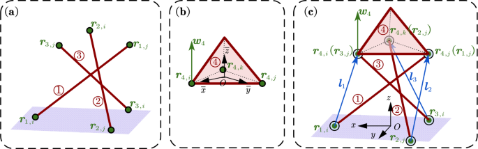

  

  Illustration of the demonstrative tensegrity structure. (a) Three rigid bars , , and ; (b) a tetrahedral rigid body ; (c) a tensegrity with ball-jointed rigid members and tensile cables

  Each rigid bar has a length $l = 0.22$ m, a virtual radius of cross-section $r = 1.833 \times 10^{-3}$ m, and a uniform density $\rho = 630$ kg/m³. According to Sect. 2.3, the mass matrix of each rigid bar is given by

  $$ \boldsymbol{M}_{I} = \begin{bmatrix} {0.000\,487\,8} & {0.000\,243\,9} \\ {0.000\,243\,9} & {0.000\,487\,8} \end{bmatrix} \otimes \mathbf{I}_{3} \text{ for } I = 1,2,3. $$

  (53)

• Step 2. Description of the tetrahedral rigid body

  Figure 8(b) shows the tetrahedral rigid body as another building block for the whole structure. According to Sect. 2.1.1, there are four types of natural coordinates to be used. Anticipating the next step, which will deal with ball joints, it is convenient to use the “rrrw” type natural coordinates $\boldsymbol{q}_{4,\mathrm{rrrw}} = [\boldsymbol{r}_{4,i}^{\mathrm{T}},\boldsymbol{r}_{4,j}^{ \mathrm{T}},\boldsymbol{r}_{4,k}^{\mathrm{T}},\boldsymbol{w}_{4}^{\mathrm{T}}]^{ \mathrm{T}}$, which consist of three basic points located at the lower three vertices of the tetrahedron and the automatically generated base vector $\boldsymbol{w}_{4}$.

  The tetrahedron has a height $h = {0.070\,71}$ m, a circumradius $R = {0.07}$ m for the base triangle, above which the mass center is located at $\bar{\boldsymbol{r}}_{g} = [0.0, 0.0, 0.0148229]~\text{m}$. The mass and inertia matrix are given by, respectively, $m = {0.2999}$ kg and $\bar{\boldsymbol{I}}= \mathrm{diag}\left ( {0.7664}, {0.7664}, {1.246} \right ) \times 10^{-3}~{\mathrm{kg\,m^{2}}}$. According to Sect. 2.3, the mass matrix of the tetrahedral rigid body is given by

  $$ \boldsymbol{M}_{4} = \begin{bmatrix} {0.089\,85} & {0.005\,060} & {0.005\,060} & {0.1164} \\ {0.005\,060} & {0.089\,85} & {0.005\,060} & {0.1164} \\ {0.005\,060} & {0.005\,060} & {0.089\,85} & {0.1164} \\ {0.1164} & {0.1164} & {0.1164} & {1.290} \end{bmatrix} \otimes \mathbf{I}_{3}. $$

  (54)

• Step 3. Description of ball joints

  Utilizing the flexibility of the proposed modeling method, ball joints can be described conveniently without introducing additional constraints. Referring to Fig. 8(c), there are two kinds of ball joints.

  • (a) The first kind connects the upper ends of the bars to the tetrahedral rigid body. According to Sect. 3.1, they can be described by sharing the basic points. Consequently, the natural coordinates for the tetrahedral rigid body are replaced by

    $$ \boldsymbol{q}_{4,\mathrm{rrrw}} = [ \boldsymbol{r}_{3,j}^{\mathrm{T}}, \boldsymbol{r}_{1,j}^{ \mathrm{T}}, \boldsymbol{r}_{2,j}^{\mathrm{T}}, \boldsymbol{w}_{4}^{\mathrm{T}} ]^{ \mathrm{T}}. $$

    (55)

  • (b) The second kind connects the lower ends of the bars with the ground, constituting boundary conditions. According to Sect. 3.2, they can be described by specifying the matrices

    $$ \begin{aligned} &\tilde{\boldsymbol{E}}_{I} = \begin{bmatrix} 1 & 0 & 0 & 0 & 0 & 0 \\ 0 & 1 & 0 & 0 & 0 & 0 \\ 0 & 0 & 1 & 0 & 0 & 0 \end{bmatrix} \text{ and} \\ &\check{\boldsymbol{E}}_{I} = \begin{bmatrix} 0 & 0 & 0 & 1 & 0 & 0 \\ 0 & 0 & 0 & 0 & 1 & 0 \\ 0 & 0 & 0 & 0 & 0 & 1 \end{bmatrix} \text{ for } I = 1,2,3. \end{aligned} $$

    (56)

    Consequently, the free coordinates for rigid bars are given by $\check{\boldsymbol{q}}_{I} = \check{\boldsymbol{E}}_{I}\boldsymbol{q}_{I,\mathrm{rr}} = \boldsymbol{r}_{I,j}$, $I = 1,2,3$.

• Step 4. Description of the system coordinates and mass matrix

  At this point, the prescribed, free, and total coordinates for the entire system can be determined as

  $$ \begin{aligned} \tilde{\boldsymbol{q}} &= \begin{bmatrix} \boldsymbol{r}_{1,i}^{\mathrm{T}}, \boldsymbol{r}_{2,i}^{\mathrm{T}}, \boldsymbol{r}_{3,i}^{ \mathrm{T}}, \end{bmatrix}^{\mathrm{T}}, \\ \check{\boldsymbol{q}} &= \begin{bmatrix} \boldsymbol{r}_{1,j}^{\mathrm{T}}, \boldsymbol{r}_{2,j}^{\mathrm{T}}, \boldsymbol{r}_{3,j}^{ \mathrm{T}}, \boldsymbol{w}_{4}^{\mathrm{T}} \end{bmatrix}^{\mathrm{T}}, \\ \boldsymbol{q} &= \begin{bmatrix} \boldsymbol{r}_{1,i}^{\mathrm{T}}, \boldsymbol{r}_{1,j}^{\mathrm{T}}, \boldsymbol{r}_{2,i}^{ \mathrm{T}}, \boldsymbol{r}_{2,j}^{\mathrm{T}}, \boldsymbol{r}_{3,i}^{\mathrm{T}}, \boldsymbol{r}_{3,j}^{\mathrm{T}}, \boldsymbol{w}_{4}^{\mathrm{T}} \end{bmatrix}^{\mathrm{T}}. \end{aligned} $$

  (57)

  We can see that the justified usage of the sharing basic points and the prescribed coordinates greatly simplifies the description of the ball joints. As a result, 12 free coordinates and 9 intrinsic constraints (1 for each bar and 6 for the rigid body) will become the unknowns in the dynamic equation. No extrinsic constraints are required.

  The system separation matrices $\tilde{\boldsymbol{E}}$ and $\check{\boldsymbol{E}}$ and the selection matrices for rigid members in (19) can be expressed explicitly. For example, we have

  $$ \begin{aligned} & \boldsymbol{T}_{1} = \begin{bmatrix} 1 & 0 & 0 & 0 & 0 & 0 & 0 \\ 0 & 1 & 0 & 0 & 0 & 0 & 0 \end{bmatrix} \otimes \mathbf{I}_{3} \text{ and}\\ & \boldsymbol{T}_{4} = \begin{bmatrix} 0 & 0 & 0 & 0 & 0 & 1 & 0 \\ 0 & 1 & 0 & 0 & 0 & 0 & 0 \\ 0 & 0 & 0 & 1 & 0 & 0 & 0 \\ 0 & 0 & 0 & 0 & 0 & 0 & 1 \end{bmatrix} \otimes \mathbf{I}_{3} \end{aligned} $$

  (58)

  for the rigid bar and the tetrahedron , respectively.

  Furthermore, the system mass matrices $\boldsymbol{M}=\sum _{I=1}^{n_{b}}\boldsymbol{T}_{I}^{\mathrm{T}}\boldsymbol{M}_{I}\boldsymbol{T}_{I}$ can be easily assembled.

• Step 5. Desciption of the cables and tensile forces

  Referring to Fig. 8(c), tensile cables are added to connect the lower end of rigid bars and the lower vertices of the tetrahedron. For example, the vector $\boldsymbol{l}_{1}$ representing the first cable is formulated by (23) as

  $$ \begin{aligned} \boldsymbol{l}_{1} = \boldsymbol{r}_{4,i} - \boldsymbol{r}_{1,i} = \boldsymbol{C}_{4,i} \boldsymbol{T}_{4}\boldsymbol{q}-\boldsymbol{C}_{1,i}\boldsymbol{T}_{1}\boldsymbol{q} = \boldsymbol{J}_{1}\boldsymbol{q}. \end{aligned} $$

  (59)

  We can see that this formula is valid regardless of the type of rigid members to which the cable connects, thanks to the unifying form (9). Then, the generalized tension force $\check{\boldsymbol{Q}}$ of the system can be derived, following the rest of Sect. 3.4, where the selection matrices (58) automatically take care of the sharing coordinates.

  Each cable has a stiffness coefficient $\kappa = 1 \times 10^{3}$ N/m, a damping coefficient $\eta = 2$ Ns/m, and a rest length $\mu = 0.05$ m.

• Step 6. Dynamic equations and dynamic analysis

  Using the above intermediate results, the formulation of the dynamic equations (30a)–(30b) becomes straightforward. Typically, the system is analyzed in three steps:

  • (a) Seek the static equilibrium configuration of the system by solving the inverse statics problem (33) or by solving a dynamic relaxation problem.

  • (b) Determine the stability and natural frequencies of the system by solving the eigenvalue problem (39) of the linearized dynamic equation.

  • (c) Study the nonlinear dynamic response of the system by solving the nonlinear dynamic equation (30a)–(30b) using the proposed MSI scheme.

  Here we directly perform step (c) with a timestep size $h=1 \times 10^{-3}$ m for 1 second. Figure 9 plots the trajectory of the point $\boldsymbol{r}_{4,i}$, showing that the dynamic responses are vibrational and are slowly damped as time progresses.

  Fig. 9

  

  Time histories of the trajectory of the point $\boldsymbol{r}_{4,i}$ in the $x$-, $y$-, and $z$-directions, respectively

5.2 Example 2: a fusiform tensegrity structure

This example considers a three-dimensional fusiform tensegrity structure, involving a punctured square rigid board and a rigid bar. In a study of topology-finding method [27], this structure represents one of the simplest Class-1 general tensegrities. A variant of this structure, which replaces the punctured square with a triangle, is studied by Liu et al. [26] as a tensegrity robot. However, due to difficulties arising from the heterogeneity of rigid members, the dynamic characteristics of this structure were not studied in the above references. To demonstrate its rich dynamic motions, an initially unbalanced configuration, where the rigid board is rotated around the $x$-axis by 45°, and the rigid bar is rotated around the $y$-axis by 15°, is shown in Fig. 10(b). Both rigid members are given a uniform density $\rho =630$ kg m⁻¹, corresponding to teak wood. All eight cables have a stiffness coefficient $\kappa = 100$ N m⁻¹ with no damping. The upper four cables are given the rest length $\mu = 0.05$ m, whereas the lower four ones have $\mu = 0.1$ m. The structure is free-floating.

Fig. 10

(a) Dimensions of a rigid square board; (b) initial configuration of a fusiform tensegrity structure composed of a rigid bar and a rigid square board

Consider 100-second long-time simulations with timestep $h = 1 \times 10 ^{-3}$ s, carried out by the MSI scheme and the generalized-$\alpha$ scheme [60]. Figure 11 visualizes the structural movements, whereas Fig. 12 compares the trajectories of the marker point and the mechanical energy $E=T+V$ produced by the two schemes. These results show that the motions of a 3D rigid bar are correctly described by the natural coordinates without any difficulty and that the trajectories between the two schemes are very close in the beginning of the simulations. In particular, the MSI scheme conserves the mechanical energy $E$ and obtains vibrations between the two rigid members throughout the entire process. In contrast, the generalized-$\alpha$ scheme with $\rho _{\infty}=0.7$ gradually damps out such high-frequncy vibrations and dissipates the associated energy. Therefore the MSI scheme is more suitable to faithfully simulate the long-time dynamics of general tensegrity structures.

Fig. 11

Snapshots of the fusiform tensegrity structure at different time instances simulated by (a,b,c,d,e) the MSI scheme and (f,g,h,i,j) the generalized-$\alpha$ scheme. Blue dots indicate the marker point (Color figure online)

Fig. 12

(a) Trajectories of the marker point in the $y$-direction and (b) time histories of the mechanical energy $E$ given by the MSI scheme and generalized-$\alpha$ scheme

5.3 Example 3: a tensegrity bridge

This example is a Class-1 tensegrity bridge composed of a rectangular rigid body as the bridge deck and inclined rigid bars as supporting struts, as shown in Fig. 13. It represents another example resulting from the design method of topology-finding [27]. Because the bars have no contact with the deck, it is a Class-1 tensegrity structure. Each rigid bar has a length $l = 15.95$ m and a virtual radius of cross-section $r = 0.13$ m, and the deck has dimensions $24~\text{m}\times 6~\text{m}\times 0.25~\text{m}$ (length × width × height). Note that material properties were not considered in the above reference. For demonstration purpose, rigid members are given a uniform density of teak wood $\rho = 630$ kg/m³, and cables are given a stiffness coefficient $\kappa = 25.92$ kN m⁻¹. Furthermore, the lower end of each bar is fixed to the ground, so that the structure can support self-weight and loading forces.

Fig. 13

Schematic figures of the tensegrity bridge from (a) left view, (b) top view, and (c) oblique view with a concentrated loading force. Blue dots indicate the marker point (Color figure online)

Due to the heterogeneity between rigid bodies and rigid bars, it is difficult to obtain reference results for the dynamic behaviors of the bridge in commercial software that uses minimal coordinates, such as Adams. Therefore, to validate the dynamic formulations and the MSI scheme, the resonance phenomenon will be simulated. Firstly, a static equilibrium configuration and the rest lengths of cables are sought by the geodesic dynamic relaxation method [62]. Then linearized dynamic analysis is performed to compute the natural frequencies and mode shapes, which reveal how the structure vibrates around the initial static equilibrium. The first four vibration modes are shown in Fig. 14. In particular, a tilting movement of the deck can be observed from the second mode with a natural frequency 0.553 Hz. Based on this observation, the nonlinear dynamics simulations can be validated by inducing vibrations resonating with this frequency. To this end, a concentrated loading force $\boldsymbol{f}(t)$ with different frequencies is exerted to the edge of the deck, as shown in Fig. 13(c). The force magnitude is a function of time $f(t)= 2\times 10^{4}\left ( \sin \left (2\pi \nu t\right ) + 1\right )$ N, where $\nu = 0.453, 0.553, 0.653$ Hz are three excitation frequencies, representing three simulation cases. Nonlinear dynamic simulations for 10 seconds are performed for each case with timestep $h = 1 \times 10^{-2}$ s, using the MSI scheme. Trajectories of the loading point in the $z$-direction is plotted in Fig. 15. It shows that the amplitude of response is significantly increased only for $\nu = 0.553$ Hz, indicating vibrations resonant with the second mode and hence validates the proposed modeling formulations and integration scheme.

Fig. 14

The mode shapes and natural frequencies for the first four vibration modes of the tensegrity bridge. The configuration of static equilibrium is colored in gray for reference (Color figure online)

Fig. 15

Trajectories of the loading point in the $z$-direction for the three simulation cases with different excitation frequencies

5.4 Example 4: a tensegrity structure designed by embedding

5.4.1 Structural design using the “embedding” method

Besides using algorithmic methods such as topology-finding, intuitive methods are also viable to design general tensegrity structures. One such method can be called “embedding” as exemplified by Fig. 16. Firstly, the design process starts with known primitive tensegrities, such as a rotatable Class-2 tensegrity with two tetrahedrons in contact (Fig. 16(a)), and a deployable two-stage tensegrity prism (Fig. 16(b)). Secondly, the latter one can be embedded into the former one, replacing the ball joint (Fig. 16(c)). Lastly, multiple modules can be stacked sequentially to build multistage structures (Fig. 16(d,e)). In this way, the new structure is a Class-3 tensegrity endowed with the rotatable and deployable functionalities of the primitives.

Fig. 16

Schematic figures of (a,b) the primitive tensegrities, (c) a “embedded” tensegrity structure, and a 4-stage “embedded” tensegrity structure in the (d) folded and (e) unfolded configurations (Color figure online)

Note that the “embedding” method is akin to the concept of “self-similar” iterations (see, for example, [3]) but not limited to “bars-only” compressive tensegrity structures. Further in-depth investigations are still needed to broaden the applications of the “embedding” method, but those are beyond the scope of this paper.

The structural properties are as follows. Each rigid bar has a length $l = 0.14$ m and a virtual radius of cross-section $r = 1.167 \times 10^{-3}$ m, and the triangular rigid plate has a side length $l = 0.2939$ m and a height $h = 0.01$ m. All rigid members are given a uniform density of teak wood $\rho = 630$ kg/m³, and tensile cables are given a stiffness coefficient $\kappa = 25.92$ kN m⁻¹. Furthermore, to support the self-weight of the structure, the lowermost plate is fixed to the ground by giving boundary conditions.

5.4.2 Determining the cable-based actuation values

Deployments of the structure are achieved by cable-based actuation [59, 63], which is implemented by timely changing the rest lengths of the cables $\boldsymbol{\mu}$. In other words, the variables $\boldsymbol{\mu}(t)$ in the dynamic equations (30a)–(30b) are specified as a time-dependent function during the simulation. As time progresses, the internal unbalanced tensile forces due to varied rest lengths cause the structure to move.

To ensure that the structure reaches the desired configuration and a smooth transition during the deployment process, the actuation values $\boldsymbol{\mu}(t)$ are determined by the following steps:

• 1. Specify the reference configurations of the tensegrity structure as shown in Fig. 16(d,e), which consist of the positions and orientations of all the rigid members.

• 2. Specify the rest lengths of inactive cables. In this example, the cables belonging to the inner prisms are considered active, whereas the outer cables of each stage are considered inactive, which are given predefined rest lengths 0.17 m, 0.15 m and 0.19 m.

• 3. Establish an inverse statics problem (33) with minimum force constraints and solve for the rest lengths of the active cables. For the folded configure, Fig. 16(d), the results are shown in $\mu _{\mathrm{diagnal}} = {0.050\,66}$ m, $\mu _{\mathrm{middle}} = {0.1390}$ m. For the unfolded configuration, Fig. 16(e), we have $\mu _{\mathrm{diagnal}} = {0.1024}$ m, $\mu _{\mathrm{middle}} = {0.069\,38}$ m.

• 4. Construct the time-dependent actuation function $\boldsymbol{\mu}(t)$ by interpolating between the calculated rest lengths corresponding to different reference configurations of the structure. For demonstration purposes, the function $\boldsymbol{\mu}(t)$ is constructed such that the active cables are released in a stage-by-stage manner, as shown in Fig. 17.

  Fig. 17

  

  The time-dependent interpolation functions of the tensile cables’ rest lengths $\boldsymbol{\mu}(t)$ (Color figure online)

5.4.3 Dynamic simulation of the deployment process

Before simulating the deployment process, it is necessary to determine the initial configuration of the structure. To this end, the geodesic dynamic relaxation method [62] is used to obtain the initial configuration, which is in static equilibrium under the tension loads and external loads (e.g., gravity), as shown in Fig. 18(a). The dynamic process of the system is then simulated by the proposed MSI scheme with time step size $h = 4 \times 10^{-3}$ s over a time span of 60 s.

Fig. 18

Snapshots of the 4-stage “embedded” tensegrity structures during cable-based deployment. Blue dots indicate the marker point (Color figure online)

During the simulation, the structure’s rest lengths are adjusted according to the interpolated time-dependent functions (Fig. 17), resulting in a stage-by-stage deployment of the structure. Additionally, the uneven tensions of the outer cables induce the structure to move in an asymmetric inclination, which is more prominent in the unfolded configuration (Fig. 18(b-e)) than in the folded configuration for an analysis of how the actuations influence the movement and stability of the structure. Figure 19 plots the trajectories of the marker point in the deployment process, showing that small vibrations occur during the dynamic deployment due to rigid-tensile coupling. The reduction of such vibrations is subject to further research.

Fig. 19

Trajectories of the marker point in (a) $x$-, (b) $y$-, and (c) $z$-directions

5.5 Example 5: a tensegrity structure designed by interfacing

5.5.1 Structural design by the “interfacing” method

Another intuitive design methods can be called “interfacing”, as exemplified by Fig. 20. Consider again the two tensegrity primitives in Example 4, as shown in Fig. 20(a,c). Additionally, a spine-like tensegrity primitive [64], composed of two tetrahedrons and six cables, are introduced as an interface to connect the former two, leading to a new multistage tower-like structure Fig. 20(d,e). In this way, the new structure also acquires the ability of rotations and deployments, albeit at different stages. The advantage of the “interfacing” method is that it can extend an existing structure, without altering its internal topology. Thus it automatically leads to modular structure designs and can be easily combined with other methods, such as topology-finding and the “embedding” method.

Fig. 20

Schematic figures of (a,b,c) the primitive tensegrities, the (d) initial and (e) target configurations of the tower-like tensegrity structure designed by interfacing (Color figure online)

The structural properties are as follows. Each rigid bar has a length $l = 0.22$ m, a virtual radius of cross-section $r = 1.833 \times 10^{-3}$ m, and a uniform density $\rho = 630$ kg/m³. Each tetrahedron has a height $h = 0.07071$ m, a circumradius $r = 0.1$ m for the base triangle, with mass $m = 0.2999$ kg, and inertia matrix $\bar{\boldsymbol{I}}= \mathrm{diag}\left ( {0.7664}, {0.7664}, {1.246} \right ) \times 10^{-3}$ kg m². Tensile cables in the prism are given the stiffness coefficient $\kappa = 1 \times 10^{3}$ N m⁻¹. Otherwise, $\kappa = 5 \times 10^{2}$ N m⁻¹. All tensile cables have the same damping coefficient $\eta = 2$ N m⁻¹ s⁻¹. The lower ends of the tensegrity prism are fixed to the ground.

5.5.2 Determining the resonance frequencies

During the deployment process, the natural frequencies of the structure are also varied continuously. This fact allows us to validate the dynamic formulations and the MSI scheme by simulating the resonance phenomenon. To this end, the expected resonance frequencies are determined in the following steps.

• 1. Obtain the two static equilibrium configurations (Fig. 20(d,e)) with different cable rest lengths using the geodesic dynamic relaxation method [62]. These two static equilibria will be referred to as the initial and target states for the deployment process.

• 2. Linearize the dynamics of the structure around the two static equilibrium states according to Sect. 4.2.

• 3. Solve the generalized eigenvalue problem (39). The resulting lowest natural frequencies for these two states are $\xi = 1.255$ Hz and $\xi = 0.8289$ Hz, respectively. The first three vibration modes of the target state are calculated by (41) and shown in Fig. 21. We can observe that the first two modes (Fig. 21(a,b)) correspond to bending movements in the $x$- and $y$-directions, whereas the third mode (Fig. 21(c)) corresponds to the torsional movement along the $z$-direction.

  Fig. 21

  

  The mode shapes of the first three vibration modes of the tower-like tensegrity structure in target configuration. The configuration of static equilibrium is colored in gray for reference (Color figure online)

5.5.3 Dynamic simulation of the deployment process

In the dynamic simulation of the deployment process, the ground under the structure is subject to a seismic wave in the $x$-direction $x(t) = 0.003 \sin (\nu 2\pi t)$ m, where $\nu$ is the seismic frequency. According to the results obtained in Sect. 5.5.2, it is expected that resonances would occur during deployment if the seismic frequency $\nu$ is within the range $\left [{0.8289}, {1.255}\right ]$ Hz.

To verify this prediction, cable-based deployment simulations are carried out with three different seismic frequencies $\nu = 0, 0.7, 1.0$ Hz. An 80-second simulation with 60-second deployment time is carried out. Trajectories of the marker point are plotted in Fig. 22. It shows that the amplitude of response in the $x$-direction is significantly increased only for $\nu =1.0$ Hz, verifying our prediction. In fact, the resonant vibrations are large enough to cause cable-slacking, as shown in Fig. 23(b). To sum up, these results validate the proposed approach and demonstrate its efficacy in dealing with complex conditions, including slack cables, cable-based deployment, and moving boundary conditions.

Fig. 22

(a) Trajectories of the marker point in the $x$-direction and (b) the enlargement view for the three deployment cases (Color figure online)

Fig. 23

Snapshots of the tower-like tensegrity structure during deployment with seismic frequency $\nu =1.0$ Hz. Dash blue lines indicate slack cables. The deployment on static ground is colored in gray for reference in (b). Blue dots indicate the marker point (Color figure online)

5.6 Discussion

In this section, five examples were presented for demonstrating the effectiveness of the proposed approach.

These examples range from simple mechanisms to full-scale bridge and multistage deployable structures. Therefore they demonstrate the broad applicability of the proposed approach and encourage collaboration between different engineering disciplines, including civil engineering, aerospace engineering, and robotics. In particular, Examples 4 and 5 demonstrate the “embedding” and “interfacing” methods as two intuitive methods to build innovative, scalable, and deployable tensegrity structures that were not previously conceived in the literature. Therefore they represent important directions in further research in the practical design of tensegrity structures, such as large-scale space structures.

The innovations in the examples are made possible only by the two main contributions of the proposed approach. The first is the fully nonminimal description that covers the heterogeneous rigid members by offering the flexibility to arrange basic points and base vectors. The second is the unified formulation of the tension forces of cables based on polymorphism and conversion matrices. These two aspects are best demonstrated by Example 1, where the complexity of tensioned, boundary-conditioned, ball-jointed rigid bodies and rigid bars are easily handled by the proposed method.

The advantages of the nonminimal methods in previous works of “bars-only” tensegrity structures [33–37] are retained. Namely, the dynamic formulations are free from trigonometric terms, having an elegant form of DAEs with a constant mass matrix and linear dependence on the cable variables. These features mean that the established dynamic control scheme problems [19, 38] for “bars-only” tensegrity structures can be ported to general tensegrity structures with little effort.

Since the proposed dynamic formulations lead to a set of DAEs, the correct treatments of algebraic constraints are crucial to obtain accurate results of linearized and nonlinear dynamic analysis problems. For modal analysis of the linearized dynamics around static equilibrium, the reduced-basis method is used to obtain the correct natural frequencies and modal shapes. For the numerical integration of constrained nonlinear dynamics, while the existing methods in the tensegrity literature predominantly employ the constraint correction method [65, 66], in this paper, we propose the MSI scheme that directly solves the discretized DAEs, such that the constraints are satisfied at every time step and longtime simulations are accurate. Compared to the original Zu-class symplectic schemes [51, 52], the proposed MSI scheme can accommodate nonconservative forces and boundary conditions, thereby ensuring the applicability and robustness to a broad range of tensegrity dynamics.

6 Summary, conclusions, and future directions of research

In this paper, we develop a unified approach for dynamic analysis of general tensegrity structures. Our method consists of a fully nonminimal description based on natural coordinates, a unified formulation of tension forces using polymorphism and conversion matrices, and a modified symplectic integration (MSI) scheme for numerical simulations of constrained nonlinear dynamics. The effectiveness and broad applicability of this approach were demonstrated through five diverse examples, from simple mechanisms to complex deployable structures.

The key conclusions are as follows. The heterogeneity between 6-DoF rigid bodies and 5-DoF rigid bars is resolved by the nonminimal description of natural coordinates. Four and two types of natural coordinates are derived for a 3D rigid body and a rigid bar, offering the flexibility to arrange basic points and base vectors. The idea of polymorphism unifies different types of coordinates and thereby facilitates the formulations for ball joints, boundary conditions, and cables’ tension forces for general tensegrity structures. The resulting dynamic equation has a constant mass matrix and is free from trigonometric functions. Using the reduced-basis method, the governing DAEs can be linearized around static equilibrium and then reduced to a linear system for modal analysis. The one-timestep MSI scheme not only yields realistic results for energy and vibrations in long-time simulations, but also accommodates nonconservative forces and boundary conditions. Five representative numerical examples are presented. Example 1 provides a detailed step-by-step demonstration of the proposed approach. Examples 2 and 3 are general tensegrity found in the topology-finding literature, whereas Examples 4 and 5 are novel multifunctional structures created by two intuitive ways, namely the “embedding” and “interfacing” methods. Various complex situations, including dynamic external loads, cable-based deployment, and moving boundaries, demonstrate the efficacy of the proposed approach for the dynamic analysis of general tensegrity structures.

Regarding future research directions, the proposed approach can be extended to include massive cables. In this direction, the cable’s mass can be distributed as point masses associated with the cable’s nodes [37]. In the simplest case, which assumes no lateral displacement of the cable [59], the cable’s point mass can be included in the mass matrices of the rigid members. Furthermore, sliding cables with clustered actuation [67–70] can also be considered. These clustered cables can slide through pulleys on the rigid members, thereby reducing the number of driving motors at the expense of increasing the coupling across multiple modules of the entire tensegrity structure. Finally, the linear dependence on cables’ force densities (26) can be exploited for optimization the structural stiffness under external loads [29, 71–73] and the design of control schemes [19], aiming to integrate structure and control design as for classical tensegrity systems [74].

References

Buckminster, F.R.: Tensile-Integrity Structures. US3063521A, November 1962
Lalvani, H.: Origins of tensegrity: views of Emmerich, Fuller and Snelson. Int. J. Space Struct. 11(1–2), 27 (1996)
Skelton, R.E., de Oliveira, M.C.: Tensegrity Systems. Springer, NY (2009)
Skelton, R.E., Adhikari, R., Pinaud, J.-P., Chan, W., Helton, J.W.: An introduction to the mechanics of tensegrity structures. In: Proceedings of the 40th IEEE Conference on Decision and Control (Cat. No. 01CH37228), vol. 5, pp. 4254–4259. IEEE, Orlando (2001)
Krishnan, S., Li, B.: Design of lightweight deployable antennas using the tensegrity principle. In: Earth and Space 2018, pp. 888–899. American Society of Civil Engineers, Cleveland (2018)
Furuya, H.: Concept of deployable tensegrity structures in space application. Int. J. Space Struct. 7(2), 143–151 (1992)
Sultan, C., Skelton, R.: Deployment of tensegrity structures. Int. J. Solids Struct. 40(18), 4637–4657 (2003)
Sultan, C.: Chap. 2 tensegrity: 60 years of art, science, and engineering. In: Advances in Applied Mechanics, vol. 43, pp. 69–145. Elsevier, Amsterdam (2009)
Sychterz, A.C., Smith, I.F.C.: Using dynamic measurements to detect and locate ruptured cables on a tensegrity structure. Eng. Struct. 173, 631–642 (2018)
Veuve, N., Safaei, S.D., Smith, I.F.C.: Deployment of a tensegrity footbridge. J. Struct. Eng. 141(11), 04015021 (2015)
Tibert, A.G., Pellegrino, S.: Deployable tensegrity reflectors for small satellites. J. Spacecr. Rockets 39(5), 701–709 (2002)
Zolesi, V.S., Ganga, P.L., Scolamiero, L., Micheletti, A., Podio-Guidugli, P., Tibert, G., Donati, A., Ghiozzi, M.: On an innovative deployment concept for large space structures. In: 42nd International Conference on Environmental Systems. American Institute of Aeronautics and Astronautics (2012)
Sultan, C., Corless, M., Skelton, R.T.: Peak-to-peak control of an adaptive tensegrity space telescope. In: Smart Structures and Materials 1999: Mathematics and Control in Smart Structures, vol. 3667, pp. 190–201. International Society for Optics and Photonics, California (1999)
Sabelhaus, A.P., Li, A.H., Sover, K.A., Madden, J.R., Barkan, A.R., Agogino, A.K., Agogino, A.M.: Inverse statics optimization for compound tensegrity robots. IEEE Robot. Autom. Lett. 5(3), 3982–3989 (2020)
Luo, J., Wu, Z., Xu, X., Chen, Y., Liu, Z., Ming, L.: Forward statics of tensegrity robots with rigid bodies using homotopy continuation. IEEE Robot. Autom. Lett. 7(2), 5183–5190 (2022)
Bruce, J., Caluwaerts, K., Iscen, A., Sabelhaus, A.P., SunSpiral, V.: Design and evolution of a modular tensegrity robot platform. In: 2014 IEEE International Conference on Robotics and Automation (ICRA), pp. 3483–3489. IEEE, Hong Kong (2014)
Chen, B., Jiang, H.: Swimming performance of a tensegrity robotic fish. Soft Robot. 6(4), 520–531 (2019)
Sabelhaus, A.P., Ji, H., Hylton, P., Madaan, Y., Yang, C., Agogino, A.M., Friesen, J., SunSpiral, V.: Mechanism design and simulation of the ULTRA spine: a tensegrity robot. In: International Design Engineering Technical Conferences and Computers and Information in Engineering Conference, vol. 57120, pp. 05–08059. American Society of Mechanical Engineers, Massachusetts (2015)
Chen, M., Liu, J., Skelton, R.E.: Design and control of tensegrity morphing airfoils. Mech. Res. Commun. 103, 103480 (2020)
Chen, M., Goyal, R., Majji, M., Skelton, R.E.: Design and analysis of a growable artificial gravity space habitat. Aerosp. Sci. Technol. 106, 106147 (2020)
Snelson, K.: The art of tensegrity. Int. J. Space Struct. 27(2–3), 71–80 (2012)
Levin, S.M.: The tensegrity-truss as a model for spine mechanics: biotensegrity. J. Mech. Med. Biol. 2(03n04), 375–388 (2002)
Lessard, S., Bruce, J., Jung, E., Teodorescu, M., SunSpiral, V., Agogino, A.: A lightweight, multi-axis compliant tensegrity joint. In: 2016 IEEE International Conference on Robotics and Automation (ICRA), pp. 630–635. IEEE, Stockholm (2016)
Koohestani, K.: Form-finding of tensegrity structures via genetic algorithm. Int. J. Solids Struct. 49(5), 739–747 (2012)
Intension Designs |. Tensegrity Modeling
Liu, S., Li, Q., Wang, P., Guo, F.: Kinematic and static analysis of a novel tensegrity robot. Mech. Mach. Theory 149, 103788 (2020)
Wang, Y., Xu, X., Luo, Y.: Topology design of general tensegrity with rigid bodies. Int. J. Solids Struct. 202, 278–298 (2020)
Ma, S., Chen, M., Peng, Z., Yuan, X., Skelton, R.E.: The equilibrium and form-finding of general tensegrity systems with rigid bodies. Eng. Struct. 266, 114618 (2022)
Wang, Y., Xu, X., Luo, Y.: Self-equilibrium, mechanism stiffness, and self-stress design of general tensegrity with rigid bodies or supports: a unified analysis approach. J. Appl. Mech. 90(8), 081004 (2023)
Wroldsen, A.S., de Oliveira, M.C., Skelton, R.E.: Modelling and control of non-minimal non-linear realisations of tensegrity systems. Int. J. Control 82(3), 389–407 (2009)
Cefalo, M., Mirats-Tur, J.M.: A comprehensive dynamic model for class-1 tensegrity systems based on quaternions. Int. J. Solids Struct. 48(5), 785–802 (2011)
Sultan, C., Corless, M., Skelton, R.E.: Linear dynamics of tensegrity structures. Eng. Struct. 24(6), 671–685 (2002)
Skelton, R.: Dynamics and control of tensegrity systems. In: Gladwell, G.M.L., Ulbrich, H., GÜnthner, W. (eds.) IUTAM Symposium on Vibration Control of Nonlinear Mechanisms and Structures, vol. 130, pp. 309–318. Springer, Dordrecht (2005)
Skelton, R.E.: Efficient models of multi-body dynamics. In: Blockley, R., Shyy, W. (eds.) Encyclopedia of Aerospace Engineering, p. 301. Wiley, Chichester (2010)
Nagase, K., Skelton, R.E.: Network and vector forms of tensegrity system dynamics. Mech. Res. Commun. 59, 14–25 (2014)
Cheong, J., Skelton, R.E.: Nonminimal dynamics of general class k tensegrity systems. Int. J. Struct. Stab. Dyn. 15(02), 1450042 (2015)
Goyal, R., Skelton, R.E.: Tensegrity system dynamics with rigid bars and massive strings. Multibody Syst. Dyn. 46(3), 203–228 (2019)
Wang, R., Goyal, R., Chakravorty, S., Skelton, R.E.: Model and data based approaches to the control of tensegrity robots. IEEE Robot. Autom. Lett. 5(3), 3846–3853 (2020)
Luo, A., Xin, H., Cao, P., Hao, X., Yu, Y., Sun, P., Tian, W.: Motion simulation of six-bar tensegrity robot based on Adams. In: 2016 IEEE International Conference on Mechatronics and Automation, pp. 264–269. IEEE, Harbin (2016)
Coumans, E.: Bullet physics simulation. In: ACM SIGGRAPH 2015 Courses, p. 1 (2015)
Mirletz, B.T., Park, I., Quinn, R.D., SunSpiral, V.: Towards bridging the reality gap between tensegrity simulation and robotic hardware. In: 2015 IEEE/RSJ International Conference on Intelligent Robots and Systems (IROS), pp. 5357–5363 (2015)
Caluwaerts, K., Despraz, J., Işçen, A., Sabelhaus, A.P., Bruce, J., Schrauwen, B., SunSpiral, V.: Design and control of compliant tensegrity robots through simulation and hardware validation. J. R. Soc. Interface 11(98), 20140520 (2014)
Lessard, S., Castro, D., Asper, W., Chopra, S.D., Baltaxe-Admony, L.B., Teodorescu, M., SunSpiral, V., Agogino, A.: A bio-inspired tensegrity manipulator with multi-DOF, structurally compliant joints. In: 2016 IEEE/RSJ International Conference on Intelligent Robots and Systems (IROS), pp. 5515–5520. IEEE, Daejeon (2016)
Mirletz, B.T., Park, I.-W., Flemons, T.E., Agogino, A.K., Quinn, R.D., SunSpiral, V.: Design and control of modular spine-like tensegrity structures. In: World Conference of the International Association for Structural Control and Monitoring (IACSM), Barcalona (2014)
Friesen, J.M., Glick, P., Fanton, M., Manovi, P., Xydes, A., Bewley, T., Sunspiral, V.: The second generation prototype of a duct climbing tensegrity robot, DuCTTv2. In: 2016 IEEE International Conference on Robotics and Automation (ICRA), pp. 2123–2128 (2016)
Xu, X.M., Luo, J.H., Feng, X.G., Peng, H.J., Wu, Z.G.: A generalized inertia representation for rigid multibody systems in terms of natural coordinates. Mech. Mach. Theory 157, 104174 (2021)
De Jalón, J.G., Unda, J., Avello, A.: Natural coordinates for the computer analysis of multibody systems. Comput. Methods Appl. Mech. Eng. 56(3), 309–327 (1986)
García de Jalón, J., Unda, J., Avello, A., Jiménez, J.M.: Dynamic analysis of three-dimensional mechanisms in “natural” coordinates. J. Mech. Transm. Autom. Des. 109(4), 460–465 (1987)
de Jalón, J.G.: Twenty-five years of natural coordinates. Multibody Syst. Dyn. 18(1), 15–33 (2007)
Pappalardo, C.M.: A natural absolute coordinate formulation for the kinematic and dynamic analysis of rigid multibody systems. Nonlinear Dyn. 81(4), 1841–1869 (2015)
Zhong, W.X., Gao, Q.: Integration of constrained dynamical system via analytical structural mechanics. Int. J. Dyn. Control 4(3), 193–200 (2006)
Wu, F., Zhong, W.: Constrained Hamilton variational principle for shallow water problems and Zu-class symplectic algorithm. Appl. Math. Mech. 37(1), 1–14 (2016)
De Jalon, J.G., Bayo, E.: Kinematic and Dynamic Simulation of Multibody Systems: The Real-Time Challenge. Mechanical Engineering Series. Springer, New York (1994)
Böhm, V., Zeidis, I., Zimmermann, K.: An approach to the dynamics and control of a planar tensegrity structure with application in locomotion systems. Int. J. Dyn. Control 3(1), 41–49 (2015)
Greiner, W.: Classical Mechanics. Springer, Heidelberg (2010)
Eriksson, A., Nordmark, A.: Constrained stability of conservative static equilibrium. Comput. Mech. 64(4), 1199–1219 (2019)
Yildiz, K., Lesieutre, G.A.: Sizing and prestress optimization of class-2 tensegrity structures for space boom applications. Eng. Comput. 38, 1451–1464 (2020)
Bel Hadj Ali, N., Rhode-Barbarigos, L., Pascual Albi, A.A., Smith, I.F.C.: Design optimization and dynamic analysis of a tensegrity-based footbridge. Eng. Struct. 32(11), 3650–3659 (2010)
Kan, Z., Peng, H., Chen, B., Zhong, W.: Nonlinear dynamic and deployment analysis of clustered tensegrity structures using a positional formulation FEM. Compos. Struct. 187, 241–258 (2018)
Arnold, M., Brüls, O.: Convergence of the generalized-\(\alpha \) scheme for constrained mechanical systems. Multibody Syst. Dyn. 18(2), 185–202 (2007)
Bauchau, O.A., Epple, A., Bottasso, C.L.: Scaling of constraints and augmented Lagrangian formulations in multibody dynamics simulations. J. Comput. Nonlinear Dyn. 4, 021007 (2009)
Miki, M., Adriaenssens, S., Igarashi, T., Kawaguchi, K.: The geodesic dynamic relaxation method for problems of equilibrium with equality constraint conditions. Int. J. Numer. Methods Eng. 99(9), 682–710 (2014)
Roffman, K.M., Lesieutre, G.A.: Cable-actuated articulated cylindrical tensegrity booms. In: AIAA Scitech 2019 Forum. AIAA SciTech Forum. American Institute of Aeronautics and Astronautics, San Diego (2019)
Tietz, B.R., Carnahan, R.W., Bachmann, R.J., Quinn, R.D., SunSpiral, V.: Tetraspine: robust terrain handling on a tensegrity robot using central pattern generators. In: 2013 IEEE/ASME International Conference on Advanced Intelligent Mechatronics, pp. 261–267. IEEE, Wollongong (2013)
Cheong, J., Skelton, R.E., Cho, Y.: A numerical algorithm for tensegrity dynamics with non-minimal coordinates. Mech. Res. Commun. 58, 46–52 (2014)
Hsu, S.-C., Tadiparthi, V., Bhattacharya, R.: A Lagrangian method for constrained dynamics in tensegrity systems with compressible bars. Comput. Mech. 67(1), 139–165 (2021)
Kan, Z., Peng, H., Chen, B., Zhong, W.: A sliding cable element of multibody dynamics with application to nonlinear dynamic deployment analysis of clustered tensegrity. Int. J. Solids Struct. 130–131, 61–79 (2018)
Kan, Z., Song, N., Peng, H., Chen, B., Song, X.: A comprehensive framework for multibody system analysis with clustered cables: examples of tensegrity structures. Int. J. Solids Struct. 210–211, 289–309 (2021)
Ma, S., Chen, M., Skelton, R.E.: Dynamics and control of clustered tensegrity systems. Eng. Struct. 264, 114391 (2022)
Bel Hadj Ali, N., Kan, Z., Peng, H., Rhode-Barbarigos, L.: On static analysis of tensile structures with sliding cables: the frictional sliding case. Eng. Comput. 37(2), 1429–1442 (2021)
Shekastehband, B., Pourmand, N.: Effects of self-stress distributions on stability of tensegrity structures. Int. J. Struct. Stab. Dyn. 17(03), 1750029 (2016)
Trinh, D.T.N., Lee, S., Kang, J., Lee, J.: Force density-informed neural network for prestress design of tensegrity structures with multiple self-stress modes. Eur. J. Mech. A, Solids 94, 104584 (2022)
Ma, S., Chen, Y., Chen, M., Skelton, R.E.: Equilibrium and stiffness study of clustered tensegrity structures with the consideration of pulley sizes. Eng. Struct. 282, 115796 (2023)
Goyal, R., Majji, M., Skelton, R.E.: Integrating structure, information architecture and control design: application to tensegrity systems. Mech. Syst. Signal Process. 161, 107913 (2021)
Funding
This research was supported by the National Natural Science Foundation of China (Grant numbers 12002396, 12372053) and Shenzhen Science and Technology Program (Grant number ZDSYS20210623091808026).
Author information
Authors and Affiliations
Contributions
J. L. developed the methodology, conducted software analysis, validated the results, and wrote the original draft. X. X. conceptualized the study, conducted formal analysis, provided supervision, and contributed to writing and editing. Z. W. managed the project and contributed to writing and editing. S. W. contributed to the methodology and participated in writing and editing. All authors reviewed the manuscript.
Corresponding author
Ethics declarations
Competing interests
The authors declare no competing interests.
Additional information
Publisher’s Note
Springer Nature remains neutral with regard to jurisdictional claims in published maps and institutional affiliations.
Rights and permissions
Springer Nature or its licensor (e.g. a society or other partner) holds exclusive rights to this article under a publishing agreement with the author(s) or other rightsholder(s); author self-archiving of the accepted manuscript version of this article is solely governed by the terms of such publishing agreement and applicable law.
About this article
Cite this article
Luo, J., Xu, X., Wu, Z. et al. A unified approach to dynamic analysis of tensegrity structures with arbitrary rigid bodies and rigid bars. Multibody Syst Dyn (2024). https://doi.org/10.1007/s11044-024-10007-3
Received:
Accepted:
Published:
DOI: https://doi.org/10.1007/s11044-024-10007-3