
Abstract
We propose in this contribution to investigate the link between the dynamic gradient damage model and the classical Griffith’s theory of dynamic fracture during the crack propagation phase. To achieve this main objective, we first rigorously reformulate two-dimensional linear elastic dynamic fracture problems using variational methods and shape derivative techniques. The classical equation of motion governing a smoothly propagating crack tip follows by considering variations of a space-time action integral. We then give a variationally consistent framework of the dynamic gradient damage model. Owing to the analogies between the variational ingredients of these two models and under some basic assumptions concerning the damage band structuration, one obtains a generalized Griffith criterion which governs the crack tip evolution within the non-local damage model. Assuming further that the internal length is small compared to the dimension of the body, the previous criterion leads to the classical Griffith’s law through a separation of scales between the outer linear elastic domain and the inner damage process zone.
1 Introduction
The gradient damage model as formulated in [25] and close in essence to that elaborated by [19] is now acknowledged as a unified theoretic and computational framework for fracture evolution problems [10, 20, 24]. The link between damage and fracture can be rigorously established by global or local minimizations. On the one hand, via \(\varGamma\)-convergence arguments, the potential energy in the gradient damage model can be regarded as an elliptic regularization of the Griffith functional in the Variational Approach to Fracture [7]. The internal length \(\eta\) serves as a purely vanishing numerical parameter and the gradient damage model converges in terms of the global minimum toward the former sharp-interface fracture model. On the other hand, by exploiting the local stability and energy balance conditions when the damage field is concentrated inside a smoothly propagating thin band, authors of [29] derive an asymptotic Griffith’s law based on the energy release rate \(\overline{G}\) of the outer problem and the dissipated energy inside the damage band \(\overline{G}_{\mathrm{c}}\). The internal length receives here another physical interpretation since it achieves a separation of scales between the classic linear elastic fracture mechanics and the damage process zone undergoing a strain softening behavior.
In this paper we propose to generalize this link between gradient damage and Griffith’s theory to the dynamic setting. The major difficulty lies in the proper definition of an energy release rate and an equivalent material fracture resistance in gradient damage models. These concepts involve, generally speaking, the derivative of a certain energy with respect to the crack length, hence the damage zone evolution should be assumed to follow a specific path parametrized by the arc length. Based on an Eulerian approach, authors of [29] then identify a generalized damage-dependent Rice’s \(J\)-integral automatically induced by the variational formulation of quasi-static gradient damage models. To accomplish our objective in dynamics, we first revisit the Griffith’s linear elastic dynamic fracture mechanics theory and rigorously provide a variational interpretation of the dynamic \(J\)-integral obtained classically from an energy flux integral entering into the crack tip which balances the energy dissipated due to crack propagation [11]. We propose in Sect. 2 a Lagrangian energetic approach to the dynamic energy release rate using calculus of variations and shape optimization. The desired evolution laws for the cracked body and the crack itself automatically follow by considering variations of a space-time action integral.
It turns out this off-course journey furnishes precisely an adequate framework for deriving the crack tip equation of motion in dynamic gradient damage models. The variational formulation presented in Sect. 3 can be regarded as a generalization of the regularized dynamic fracture model [8] and the phase-field approaches originating from the computational mechanics community [6]. Under the same assumption in [29] concerning the damage band structuration and applying the same shape derivative techniques as before to a generalized space-time action integral containing the damage dissipation energy, we identify automatically a generalization of the dynamic \(J\)-integral and the dynamic energy release rate. The equation of motion of the crack tip predicted by the dynamic gradient damage model is then governed by Griffith-like scalar equations involving these concepts. This property can thus be seen as a generalization of the results obtained in [29]. With the help of a similar separation of scales in Sect. 4, the former derived generalized Griffith criterion admits also an asymptotic interpretation. Assuming that the internal length \(\eta\) is small compared to the dimension of the body, we retrieve the classical Griffith’s law of cracks involving the dynamic energy release rate of the outer problem and the material toughness defined as the amount of energy dissipated across the damage process zone.
General notation conventions adopted in this paper are summarized as follows. Scalar-valued quantities will be denoted by italic Roman or Greek letters like the crack length \(l_{t}\) or the damage field \(\alpha _{t}\). Vectors and second-order tensors will be represented by boldface letters such as the displacement field \(\mathbf{u}_{t}\) and the stress tensor \(\boldsymbol{\sigma}_{t}\). Higher order tensors considered as linear operators will be indicated by sans-serif letters: the elasticity tensor \(\mathsf{A}\) for instance. Intrinsic notation is adopted and contraction on lower-order tensors will be written without dots \(\mathsf{A}\boldsymbol{\varepsilon}_{t}=\mathsf{A}_{ijkl}\boldsymbol {\varepsilon}_{kl}\) (the summation convention is assumed). Inner products between two vectors or tensors of the same order will be denoted with a dot, such as \(\mathsf{A}\boldsymbol{\varepsilon}_{t}\cdot\boldsymbol{\varepsilon }_{t}=\mathsf{A}_{ijkl}\boldsymbol{\varepsilon}_{kl}\boldsymbol {\varepsilon}_{ij}\) (the summation convention is assumed). Time dependence will be indicated by a subscript, like \(\mathbf{u}:(t,\mathbf{x})\mapsto\mathbf{u}_{t}(\mathbf{x})\). In particular, \(\mathbf{u}_{t}\) is understood as the displacement field at time \(t\), whereas \(\mathbf{u}\) refers to the time evolution of the displacement field.
2 Variational Approach to Dynamic Fracture
As discussed in the introduction, this section will be devoted to a rigorous reformulation of an energetic approach to dynamic fracture. The basic assumptions will be a two-dimensional homogeneous and isotropic linear elastic body \(\varOmega\) containing a smoothly propagating crack \(\varGamma_{t}\) with a pre-defined path \(l\mapsto\boldsymbol{\gamma}(l)\in\mathbb{R}^{2}\) parametrized by its arc length \(t\mapsto l_{t}\geq0\). The symbol \(\mathbf{P}_{t}=\boldsymbol{\gamma}(l_{t})\) will be used to represent the crack tip at time \(t\). The current cracked configuration will be denoted by \({\varOmega\setminus\varGamma_{t}}\) on which the kinematic quantities are defined. For the sake of simplicity, the crack \(\varGamma_{t}\) is assumed to remain far from the boundary \(\partial\varOmega\). The spatial crack path \(l\mapsto\boldsymbol{\gamma}(l)\) can be curved but in this contribution we will only consider a straight crack with a constant tangent \(\boldsymbol{\gamma}'(l_{t})=\boldsymbol{\tau}_{t}=\boldsymbol{\tau}_{0}\). Generalization to a curved crack path will be briefly discussed at the end of this section.
The basic energetic ingredients of the variational formulation are defined as follows. Under the small strain hypothesis, the elastic energy is given by
where \(\mathsf{A}\) is the elasticity tensor, \(\boldsymbol{\varepsilon}\) denotes the symmetrized gradient operator which gives the linearized strain \(\boldsymbol{\varepsilon} (\mathbf{u}_{t})=\frac{1}{2}(\nabla\mathbf{u}_{t}+\nabla^{\mathsf{T}}\mathbf{u}_{t})\) when applied to the displacement vector, and \(\boldsymbol{\sigma}_{t}=\mathsf {A}\boldsymbol{\varepsilon}(\mathbf{u}_{t})\) represents the stress tensor. The kinetic energy defined on the uncracked bulk is the usual quadratic function of the velocity field modulated by the material density
The Griffith surface energy [12] illustrates the hypothesis that the crack creation is accompanied by an energy dissipation solely proportional to its area (or length in 2-d cases) with a material dependent factor \(G_{\mathrm{c}}\) called the fracture toughness. It reads in our case
Finally we define the external work potential \(\mathcal{W}_{t}\) taking into account any possible body forces or surface tractions applied on a subset \({\partial\varOmega_{F}}\) of the boundary
We suppose that they are sufficiently regular in time and in space.
2.1 Lagrangian Description in the Initial Cracked Configuration
The displacement \(\mathbf{u}_{t}\) is defined in the current crack configuration \({\varOmega\setminus\varGamma_{t}}\), consequently its total variation depends on that of the crack. A Lagrangian description of the fracture problem is thus preferred if one needs to rigorously define an energy release rate with respect to the crack length [9]. The current cracked material configuration \({\varOmega\setminus\varGamma_{t}}\) is transformed to the initial one \({\varOmega\setminus\varGamma_{0}}\) thanks to a well-defined bijection \(\boldsymbol{\phi} _{l_{t}}\) whose inverse as well as itself is differentiable, see Fig. 1. Proving existence of such diffeomorphisms may be technical [16] and consequently will be directly admitted. This bijection \(\boldsymbol{\phi}\) should not be confused with the actual deformation \(\boldsymbol{\varphi}_{t}\) of the body which takes a particular material point \(\mathbf{x}\in{\varOmega\setminus\varGamma_{t}}\) to its spatial location \(\boldsymbol{\varphi}_{t}(\mathbf{x})\) in the deformed configuration \(\boldsymbol{\varphi }_{t}({\varOmega\setminus\varGamma_{t}})\). Recall that the displacement field \(\mathbf{u}_{t}\) is defined by \(\boldsymbol{\varphi}_{t}(\mathbf{x})=\mathbf{x}+\mathbf {u}_{t}(\mathbf{x})\) for all \(\mathbf{x}\) in \({\varOmega\setminus\varGamma_{t}}\).

Definition of a diffeomorphism \(\boldsymbol{\phi}_{l_{t}}:{\varOmega\setminus\varGamma_{0}}\to {\varOmega\setminus\varGamma_{t}}\) transforming the current cracked material configuration \({\varOmega\setminus\varGamma_{t}}\) to the initial one \({\varOmega\setminus\varGamma_{0}}\). It should not be confused with the actual deformation \(\boldsymbol{\varphi}_{t}\) of the body which takes a particular material point \(\mathbf{x}\in{\varOmega\setminus\varGamma_{t}}\) to its spatial location \(\boldsymbol{\varphi}_{t}(\mathbf{x})\) in the deformed configuration \(\boldsymbol{\varphi}_{t}({\varOmega\setminus\varGamma_{t}})\)
We can explicit this domain transformation by using a virtual perturbation \(\boldsymbol{\theta}^{*}\) defined on the initial configuration [9, 16]. This virtual perturbation should verify the following
Definition 1
(Virtual perturbation)
-
1.
It is sufficiently smooth in space to satisfy the definition of a diffeomorphism.
-
2.
It represents a virtual crack advance along the current crack propagation direction, that is in our case \(\boldsymbol{\theta}^{*}(\mathbf{P}_{0})=\boldsymbol{\tau}_{0}\).
-
3.
It does not alter the crack lip shape, that is \(\boldsymbol{\theta} ^{*}\cdot\mathbf{n}=0\) on the crack lip \(\varGamma_{0}\) with \(\mathbf{n}\) the unit normal vector.
-
4.
The domain boundary remains invariant, i.e., \(\boldsymbol{\theta}^{*}=\mathbf{0}\) on \(\partial\varOmega\).
An example of such virtual perturbations is given in Fig. 2.

A particular virtual perturbation \(\boldsymbol{\theta}^{*}=\theta\boldsymbol{\tau}_{0}\) verifying Definition 1. It is obtained by solving the Laplace’s equation \(\Delta\theta=0\) inside the crown \(r\leq \lVert{\mathbf{x}^{*}-\mathbf{P}_{0}} \rVert\leq R\) with adequate boundary conditions
With an arbitrary virtual perturbation verifying Definition 1, we can thus construct the bijection between the initial and current cracked material configurations. In the particular case of a straight crack path, it reads
where \(\mathbf{x}=\boldsymbol{\phi}_{l_{t}}(\mathbf{x}^{*})\) denotes the material point \(\mathbf{x}\) in the current cracked configuration \({\varOmega\setminus\varGamma_{t}}\) associated with the material point \(\mathbf{x^{*}}\) in the initial cracked configuration \({\varOmega\setminus\varGamma_{0}}\). For notational simplicity, we will suppress its subscript by writing \(\boldsymbol{\phi}=\boldsymbol{\phi}_{l_{t}}\). The (real) displacement field \(\mathbf{u}_{t}\) will thus be pulled-back to the initial configuration via the introduced bijection by
from which along with (5) we deduce the following useful identities using the classical chain rule
As can be observed, all quantities referring to the initial material configuration \({\varOmega\setminus\varGamma_{0}}\) are indicated by a superscript \((\cdot)^{*}\). In particular, the Lebesgue integration measure in \({\varOmega\setminus\varGamma_{0}}\) will be denoted by \(\mathrm{d}\mathbf{x^{*}}\). When spatial or temporal differentiation is present, the pullback operation similar to (6) is performed first. Hence in (7), \(\nabla\mathbf{u}_{t}^{*}\) denotes the gradient of \(\mathbf{u}_{t}^{*}\) in \({\varOmega \setminus\varGamma_{0}}\), and in (8), \(\dot{\mathbf {u}}_{t}^{*}\) is understood as the time derivative of the transported displacement.
By virtue of (7) and (8), we can thus rewrite the elastic energy (1) and the kinetic (2) energy using the transported displacement
and
where we note that the transported kinetic energy functional \(\mathcal{K}^{*}\) depends on the transported displacement \(\mathbf{u}_{t}^{*}\) and the crack velocity \(\dot{l}_{t}\). Since the boundary \(\partial\varOmega\) is invariant under the transformation \(\boldsymbol{\phi}\), the external work potential (4) written in the initial configuration reads
Finally, note that we can also map the original virtual perturbation \(\boldsymbol{\theta}^{*}\) defined on the initial configuration to the current one, via a pushforward operation
All the properties discussed in Definition 1 for the initial virtual perturbation should adequately apply for the push-forwarded one by using the current crack tip \(\mathbf{P}_{t}=\boldsymbol{\phi}(\mathbf{P}_{0})\) and lip \(\varGamma_{t}\).
2.2 Reformulation Based on a Space-Time Action Integral
We suppose that the body \(\varOmega\) evolves due to an external work potential \(\mathcal{W}_{t}\) and a Dirichlet-type imposed displacement \(t\mapsto\mathbf{U}_{t}\) on a time-independent subset \(\partial\varOmega_{U}\) of the boundary. We will proceed to formulate the crack evolution equation from the (generalized) Hamilton’s principle [14], by constructing a space-time action integral similar to that introduced in [2] and then calculating directly the action variation corresponding to arbitrary virtual displacement variation and crack advance. Recall that The Principle of Least Action is formulated as a Boundary Value Problem: fix the displacement \(\mathbf{u}\) at two time ends, the real displacement evolution \(t\mapsto\mathbf{u}_{t}\) renders the action stationary.Footnote 1 Given an arbitrary interval of time \(I=[0,T]\) and the values of the (transported) displacement \(\mathbf{u}^{*}\) at both time ends noted \(\mathbf{u}^{*}_{\partial I}=(\mathbf{u}^{*}_{0},\mathbf{u}^{*}_{T})\), we will construct the admissible displacement evolution space
where the admissible function space \(\mathcal{C}_{t}\) for the current (transported) displacement at time \(t\) is an affine space of type \(\mathcal{C}_{t}=\mathcal{C}_{0}+\mathbf{U}_{t}\) with the associated vector space given by
For the admissible crack evolution, we require that the evolution of the crack tip \(t\mapsto l_{t}\) should be a non-decreasing function of time and virtual advance of the crack tip at every instant should also be non-negative to ensure irreversibility. Concretely, given an arbitrary but non-decreasing crack evolution \(t\mapsto l_{t}\), the admissible crack evolution space is given by
With the definition of the elastic energy (9), kinetic energy (10), Griffith surface energy (3) and external work potential (11) along with the admissible function spaces (12) and (13), we are now in a position to form the space-time action integral given by
which involves a generalized Lagrangian \(\mathcal{L}_{t}(\mathbf {u}^{*}_{t},\dot {\mathbf{u}}^{*}_{t},l_{t},\dot{l}_{t})\). The coupled evolution described by the couple \((\mathbf{u}^{*},l)\in\mathcal{C}(\mathbf{u}^{*})\times\mathcal{Z}(l)\) will then be governed by
Definition 2
(Variational formulation of dynamic fracture)
-
1.
Irreversibility: the crack length is a non-decreasing function of time \(\dot{l}_{t}\geq0\).
-
2.
First-order stability: the first-order action variation is non-negative with respect to arbitrary admissible displacement and crack evolutions
$$ \mathcal{A}' \bigl(\mathbf{u}^{*},l \bigr) \bigl( \mathbf{v}^{*}-\mathbf{u}^{*},s-l \bigr)\geq0\quad\text{for all }\mathbf {v}^{*}\in \mathcal{C} \bigl(\mathbf{u}^{*} \bigr)\mbox{ and all }s\in\mathcal{Z}(l). $$(15) -
3.
Energy balance: the only energy dissipation is due to crack propagation such that we have the following energy balance
$$ \mathcal{H}_{t}=\mathcal{H}_{0}+ \int_{0}^{t} \biggl( \int_{\varOmega\setminus \varGamma _{s}} \bigl(\boldsymbol{\sigma}_{s}\cdot \boldsymbol{\varepsilon}(\dot{\mathbf{U}}_{s})+\rho\ddot{ \mathbf{u}}_{s}\cdot\dot{\mathbf{U}}_{s} \bigr)\,\mathrm{d} \mathbf{x}-\mathcal{W}_{s}(\dot{\mathbf{U}}_{s})-\dot{ \mathcal{W}}_{s}(\mathbf{u}_{s}) \biggr)\,\mathrm{d}s, $$(16)where the total energy is defined by
$$ \mathcal{H}_{t}=\mathcal{E}^{*} \bigl(\mathbf{u}_{t}^{*},l_{t} \bigr)+\mathcal{S}(l_{t})+\mathcal{K}^{*} \bigl(\mathbf{u}_{t}^{*}, \dot{\mathbf{u}}_{t}^{*},l_{t},\dot{l}_{t} \bigr)- \mathcal{W}^{*}_{t} \bigl(\mathbf{u}_{t}^{*},l_{t} \bigr). $$(17)
Remark 1
We assume that the considered fields are sufficiently smooth in time and in space so that all calculations make sense. A precise statement of the functional spaces in the most general case remains beyond the scope of this paper.
In the first-order stability principle (15), the notation \(\mathcal{A}'(\mathbf{u}^{*},l)(\mathbf{v}^{*}-\mathbf {u}^{*},s-l)\) denotes the Gâteaux derivative of the action functional with respect to the displacement variation \(\mathbf{w}^{*}=\mathbf{v}^{*}-\mathbf{u}^{*}\) and crack advance \(\delta l=s-l\). Recall that the transported displacement \(\mathbf{u}_{t}^{*}\) is defined on the initial configuration \(\varOmega \setminus \varGamma _{0}\) which is fixed during the (virtual) crack increment, thanks to the introduction of the diffeomorphism \(\boldsymbol{\phi}\). The displacement variation \(\mathbf{w}^{*}\) is thus independent from that of the crack \(\delta l\), and induces automatically a variation \(\mathbf{w}\) in the current material configuration via a pushforward operation \(\mathbf{w}\circ\boldsymbol {\phi }=\mathbf{w}^{*}\).
2.3 Equivalence with the Classical Formulations
We will show in this section that the variational approach to dynamic fracture embodied by Definition 2 is equivalent to the usual wave equation in the uncracked bulk and Griffith’s law of crack evolution [11]. However, it should be noted that the variational formulation is more general. To achieve this goal, we will carefully evaluate the derivative of the action functional with respect to arbitrary displacement variation \(\mathbf{w}^{*}=\mathbf {v}^{*}-\mathbf{u}^{*}\) and crack advance \(\delta l=s-l\). Lengthy calculations are detailed in Appendices A and B and we will only present here the main results.
By firstly evaluating the action variation corresponding to zero virtual crack advance \(\delta l=s-l=0\) and using the fact that \(\mathbf {v}_{t}^{*}-\mathbf{u}_{t}^{*}=\mathbf{w}_{t}^{*}\in\mathcal{C}_{0}\) is a vector space, we obtain by virtue of the regularity hypotheses
from which the classical wave equation is deduced
We then evaluate the action derivative with zero virtual displacement variation \(\mathbf{w}^{*}=\mathbf{0}\), leading to
where the dynamic energy release rate \(G_{t}\) to be compared with the fracture toughness \(G_{\mathrm{c}}\) reads
From (20), we retrieve the desired crack stability condition which states that the dynamic energy release rate must be smaller or equal to the material fracture toughness. The consistency condition can then be derived thanks to the energy balance principle (16) and calculations in Appendix B, leading to the following Griffith’s law of crack propagation
Note that we retrieve the static energy release rate [9] by setting the velocity \(\dot{\mathbf{u}}_{t}\) and the acceleration \(\ddot{\mathbf{u}}_{t}\) in (21) to zero. A similar formula for \(G_{t}\) is obtained in [4] by constructing an ad-hoc field \(0\leq\lVert{\boldsymbol{\theta }_{t}} \rVert\leq1\) which transforms surface (line) integrals to volume (surface) integrals. Here the dynamic energy release rate \(G_{t}\) is identified by calculating the variation of the space-time action integral (14) with respect to crack increment evolution. Using the Euler-Lagrange equation
and the fact that the Lagrangian depends on the crack velocity \(\dot {l}_{t}\) solely via the kinetic energy \(\mathcal{K}^{*}\), we find the same expression for the dynamic energy release rate \(G_{t}\) as indicated in [1] and [11, p. 423]
Contrary to the quasi-static regime, this quantity \(G_{t}\) doesn’t possess the physical meaning of the derivative of the Lagrangian with respect to crack extension due to the presence of the term \((\mathrm{d}/\mathrm{d} t)(\partial\mathcal{K}^{*}/\partial\dot{l}_{t})\), as has been already noted in [22].
Although \(\boldsymbol{\theta}_{t}\) enters into the definition of \(G_{t}\) in (21), the dynamic energy release rate is independent of the exact virtual perturbation used to establish the bijection (5), owing to the following
Proposition 1
The dynamic energy release rate \(G_{t}\) is equivalent to the classical dynamic \(J\)-integral in the form of a path integral [11]
where \(\mathbf{n}\) is defined as the normal pointing out of the ball \(B_{r}(\mathbf{P}_{t})\) with \(C_{r}=\partial B_{r}(\mathbf{P}_{t})\) its boundary. As a corollary, the dynamic energy release rate (21) is independent of the virtual perturbation.
Proof
To removing any singularities near the crack tip \(\mathbf{P}_{t}\), we will partition the cracked domain \({\varOmega\setminus\varGamma_{t}}\) into the part \(\tilde {B}_{r}=B_{r}(\mathbf{P}_{t})\setminus\varGamma_{t}\) included in the ball \(B_{r}(\mathbf{P}_{t})\), and the part \(\varOmega_{r}=\varOmega\setminus (\varGamma_{t}\cup B_{r}(\mathbf{P}_{t}) )\) outside the ball, see Fig. 3. Using the following identity in \(\varOmega_{r}\)
and performing an integration by parts
the dynamic energy release rate \(G_{t}\) reads
where the second equality follows from dynamic equilibrium (19). On the last line \(\mathbf{E}_{t}\) denotes the dynamic Eshelby tensor [21]
The last term involving the body force density \(\mathbf{f}_{t}\) will have a vanishing contribution as \(r\to0\), since \(\mathbf{f}_{t}\) is supposed to be regular and asymptotically \(\mathbf{u}_{t}\) is of order \(\mathcal {O}(r^{1/2})\) in linear elastic fracture mechanics.

Partition of the cracked domain \({\varOmega\setminus \varGamma _{t}}\) using a \(\mathbf{P}_{t}\)-centered ball \(B_{r}(\mathbf{P}_{t})\) of radius \(r\)
To solve the contradiction [21] of having the Lagrangian density in (26) and the Hamiltonian density in (23), contributions from the integral on \(\tilde{B}_{r}\) must be considered. By classical singularity analysis and the steady state condition \(\dot{\mathbf{q}}_{t}\approx-\nabla\mathbf{q}_{t}\dot {l}_{t}\boldsymbol{\tau}_{t}\) verified for all (tensorial) fields \(\mathbf{q}\) near the crack tip [11], the first two terms of \(G_{t}\) in (21) are of order \(\mathcal{O}(r^{-1})\) and hence have a vanishing contribution when integrated with the area element \(r\,\mathrm{d}r\,\mathrm {d}\theta\) on \(\tilde {B}_{r}\) as \(r\) tends to zero. Similarly the term involving the body force density \(\mathbf{f}_{t}\) is not singular enough to contribute. However the last two terms \(\rho\ddot{\mathbf{u}}_{t}\cdot\nabla\mathbf {u}_{t}\boldsymbol{\theta} _{t}+\rho\dot{\mathbf{u}}_{t}\cdot\nabla\dot{\mathbf {u}}_{t}\boldsymbol{\theta }_{t}\) are integrable [22] and will yield a finite value in the limit. Using the real velocity field \(\dot{\mathbf{u}}_{t}\) in the steady state condition and the fact that \(\boldsymbol{\theta}_{t}\to \boldsymbol{\tau}_{t}\) when \(r\) becomes small due to continuity, we have
Then an integration by parts in \(\tilde{B}_{r}\) gives (noting that \(\boldsymbol{\theta}_{t}\cdot\mathbf{n}=0\) on \(\varGamma_{t}\))
from which the contribution from the last two terms in (21) can be deduced
where the last term in (27) vanishes in the limit \(r\to0\). We obtain hence
which completes the proof. □
Remark 2
Compared to the classical \(J\)-integral, the advantage of the dynamic energy release rate in the form of (21) resides in its direct usage for numerical computations with finite elements, since it involves an integral in the cells.
Remark 3
(Generalization to curved or kinked crack paths)
Let us recall that the crack \(l\mapsto\boldsymbol{\gamma}(l)\) is supposed to follow a pre-defined straight path in this paper. It can be generalized to arbitrary but smooth enough pre-defined curved paths without much technical difficulties. It suffices to carefully construct a virtual perturbation \(\boldsymbol{\theta}^{*}\) verifying Definition 1, and define the bijection \(\boldsymbol{\phi }_{t}(\mathbf{x})\) as a solution to a particular Cauchy evolution problem
see [16] for a mathematical analysis of this problem. The obtained scalar crack equation of motion will be formally the same as (22), which predicts the crack length \(l_{t}\) as a function of time along the this path. Note however that crack propagation direction should be at least continuous in time (curved path) so that the shape derivative method embodied by the diffeomorphism \(\boldsymbol{\phi}\) makes sense. In the presence of a crack kinking associated with a temporal discontinuity of the crack tangent (Fig. 4), the shape derivative methods should be adapted to capture the topology change due to the kinking [15].

Curved crack path versus kinked crack path
When the crack path is unknown, an interesting attempt is to include the crack tangent angle into the action integral (14) and evaluate the variation induced by arbitrary crack direction change. Remark that the propagation criterion derived in [2, 23] corresponds in fact to a vectorial extension of the scalar propagation law (22)
and the component perpendicular to the crack propagation direction \(\boldsymbol{\tau}_{t}\) determines the crack path.
3 Dynamic Gradient Damage Model
3.1 Variational Ingredients and Physical Principles
We present a variationally consistent formulation for dynamic gradient damage models thanks to the definition of a generalized space-time action integral similar in essence to (14) for the Griffith’s theory of dynamic fracture. Let us remain under the simplifying assumptions made in Sect. 2 and consider a two-dimensional homogeneous and isotropic body \(\varOmega\) under small strain hypothesis. Contrary to a sharp interface description of cracks, in the gradient damage approach the introduction of a continuous phase field regularizes displacement discontinuities which are now replaced by strain localizations within a finite band. Cracks are tracked with the help of a scalar damage field \(0\leq\alpha_{t}\leq1\) which introduces a smooth transition between the undamaged part \(\alpha_{t}=0\) and the crack \(\alpha_{t}=1\), see Fig. 5.

The discrete crack \(\varGamma_{t}\subset\varOmega\) regularized by a continuous damage field \(0\leq\alpha_{t}\leq1\)
Associated with an arbitrary state of the displacement \(\mathbf{u}_{t}\), the velocity \(\dot{\mathbf{u}}_{t}\) and the damage \(\alpha_{t}\), the energetic quantities needed in the following variational formulation are defined as follows. The elastic energy of the domain \(\varOmega\) is given by
where \(\mathsf{A}(\alpha)\) is the damage-dependent elasticity tensor representing stiffness degradation in the bulk from an initial undamaged state \(\mathsf{A}_{0}=\mathsf{A}(0)\) and \(\boldsymbol{\sigma}_{t}\) denotes the corresponding damage-dependent stress tensor \(\boldsymbol {\sigma }_{t}=\mathsf{A}(\alpha_{t})\boldsymbol{\varepsilon}(\mathbf{u}_{t})\). Concerning the kinetic energy, it is defined as usual by
The material density is independent of the damage, which implies total mass conservation. We now turn to the definition of the damage dissipation energy which quantifies the amount of energy consumed in the damage process. This energy is closely related to the Griffith surface energy (3) according to the \(\varGamma\)-convergence theory [7] and is defined by
with \(\eta\) an internal length of the model controlling the damage band width from a geometric point of view (see Fig. 5). In (31), \(\alpha\mapsto w(\alpha)\) denotes another damage constitutive function representing the local damage dissipation during a homogeneous damage evolution and its maximal value \(w(1)=w_{1}\) is the energy completely dissipated during such process when damage attains 1. We assume that this function \(\alpha\mapsto w(\alpha)\) along with the former stiffness degradation one \(\alpha\mapsto\mathsf{A}(\alpha)\) verify certain constitutive properties which characterize the behavior of a strongly brittle material, see [29]. Contrary to local strain-softening constitutive models, here the damage dissipation mechanism becomes non-local and localization is systematically accompanied by finite energy consumption, due to the presence of the gradient term. It can be observed that here the elastic energy (29) as well as the damage dissipation energy (31) retain their quasi-static definitions [24] since they are unaffected by dynamics.
The loading conditions and the admissible function spaces are now specified. Body forces \(\mathbf{f}_{t}\) and surface tractions \(\mathbf{F}_{t}\) applied to the body are characterized by a similar external work potential \(\mathcal{W}_{t}\) given by (4), except that the integration domain for \(\mathbf{f}_{t}\) extends to the whole body \(\varOmega \). On a subset \(\partial\varOmega_{U}\) of the boundary the body is subject to a prescribed displacement \(t\mapsto\mathbf{U}_{t}\) which is built into the definition of the admissible displacement space \(\mathcal{C}_{t}\). We suppose that the admissible displacement space is an affine space of form \(\mathcal{C}_{t}=\mathcal{C}_{0}+\mathbf{U}_{t}\) where the associated vector space \(\mathcal{C}_{0}\) is given by
Damage is here modeled as an irreversible defect evolution. Its admissible space will be built from a current damage state \(0\leq \alpha _{t}\leq1\) and it is defined by
It can be seen that a virtual damage field \(\beta_{t}\) is admissible, if and only if it is accessible from the current damage state \(\alpha_{t}\) verifying the irreversibility condition, i.e., the damage only grows. In order to formulate the temporal displacement-damage evolution as a Boundary Value Problem (Hamilton’s principle), we consider an arbitrary interval of time \(I=[0,T]\) and fix the values of \((\mathbf {u},\alpha)\) at both time ends denoted by \(\mathbf{u}_{\partial I}=(\mathbf{u}_{0},\mathbf{u}_{T})\) and \(\alpha_{\partial I}=(\alpha _{0},\alpha_{T})\), similarly to (12) and (13) in the variational formulation of the Griffith’s theory. Hence, the admissible displacement and damage evolution spaces read
With all the variational ingredients set, we are now in a position to introduce the following space-time action integral associated with an admissible pair of displacement and damage evolutions \((\mathbf {u},\alpha )\in\mathcal{C}(\mathbf{u})\times\mathcal{D}(\alpha)\)
which generalizes (14) defined for the sharp interface dynamic fracture theory. The coupled two-field time-continuous dynamic gradient damage problem can then be formulated by the following:
Definition 3
(Dynamic gradient damage evolution law)
-
1.
Irreversibility: the damage \(t\mapsto\alpha_{t}\) is a non-decreasing function of time.
-
2.
First-order stability: the first-order action variation is non-negative with respect to arbitrary admissible displacement and damage evolutions
$$ \mathcal{A}'(\mathbf{u},\alpha) (\mathbf{v}- \mathbf{u},\beta-\alpha)\geq0\quad\text{for all }\mathbf{v}\in \mathcal{C}( \mathbf{u})\mbox{ and all }\beta\in\mathcal{D}(\alpha). $$(35) -
3.
Energy balance: the only energy dissipation is due to damage
$$ \mathcal{H}_{t}=\mathcal{H}_{0}+ \int_{0}^{t} \biggl( \int_{\varOmega}\bigl(\boldsymbol{\sigma}_{s}\cdot \boldsymbol{\varepsilon}(\dot{\mathbf{U}}_{s})+\rho\ddot{ \mathbf{u}}_{s}\cdot\dot{\mathbf{U}}_{s} \bigr)\,\mathrm{d} \mathbf{x} -\mathcal{W}_{s}(\dot{\mathbf{U}}_{s})-\dot{ \mathcal{W}}_{s}(\mathbf{u}_{s}) \biggr)\,\mathrm{d}s, $$(36)where the total energy is defined by
$$ \mathcal{H}_{t}=\mathcal{E}(\mathbf{u}_{t}, \alpha_{t})+\mathcal{S}(\alpha_{t})+\mathcal{K}(\dot{ \mathbf{u}}_{t})-\mathcal{W}_{t}(\mathbf{u}_{t}). $$(37)
As can be noted, the above dynamic gradient damage model admits a similar variational framework compared to the variational approach to the Griffith’s theory of dynamic fracture summarized in Definition 2. In the quasi-static gradient damage model [25], the first-order stability condition (35) is replaced by a more restrictive stability condition. It is a physically feasible principle due to the minimization structure of static equilibrium via the definition of a potential functional. In dynamics however, we merely have a stationary action integral so only the first-order stability conditions of type (15) or (35) can be sought.
By developing the Gâteaux derivative of the action integral, further physical insights into the first-order stability condition (35) can be obtained if sufficient spatial and temporal regularities of the involved fields are assumed. Denoting the variation \(\mathbf{v}-\mathbf{u}\) by \(\mathbf{w}\) and testing (35) with \(\beta =\alpha\), we obtain after an integration by parts in the time domain
where the equality \(\mathcal{A}'(\mathbf{u},\alpha)(\mathbf {w},0)=0\) follows given that the associated linear space \(\mathcal{C}_{0}\) of \(\mathcal {C}_{t}\) is a vector space. By virtue of classical arguments of the calculus of variations, one deduces the following elastic-damage dynamic wave equation in its strong form
Compared to the classical elastic wave equation (19), here the stress tensor \(\boldsymbol{\sigma}_{t}\) is damage dependent through the definition of the elasticity tensor (29).
We now turn to the governing equation for damage evolution induced from the first-order stability condition (35). We observe that the admissible damage space \(\mathrm{D}(\alpha_{t})\) defined in (32) is convex. Due to the arbitrariness of the temporal variation of \(\beta\), testing (35) now with \(\mathbf {v}=\mathbf{u}\) gives the Euler’s inequality condition stating the partial minimality of the total energy with respect to the damage variable under the irreversible constraint for every \(t\in I\)
Although the same energy minimization principle (39) holds also for quasi-static gradient damage models [24], here the displacement field \(\mathbf{u}_{t}\) is governed by the elastic-damage wave equation (38). Developing the Euler’s inequality condition and performing an integration by parts of the damage gradient term yield a strong formulation of (39) which serves as the local damage criterion at a particular material point
For notational simplicity, the following dual variables are defined
They can be interpreted as the energy release rate density with respect to damage and the damage flux vector, see [29]. In (40), the subset \(\varGamma_{t}= \{ \mathbf{x}\in\varOmega\mid\alpha_{t}(\mathbf{x})=1 \}\) denotes the totally damaged region. We note that the local damage criterion holds only in the uncracked part of the body, since \(\beta_{t}=\alpha_{t}=1\) on \(\varGamma_{t}\) because of the definition of the admissible damage space (32). Due to the presence of the damage gradient, the criterion is described by an elliptic type equation in space involving the Laplacian of the damage. Assuming that the considered fields are also sufficiently smooth in time, the global energy balance (36) leads to the following consistency condition:
Hence damage growth is possible until a certain non-local threshold is reached. Similarly here the local consistency condition holds only in the uncracked part of the body, since \(\dot{\alpha}_{t}=0\) on \(\varGamma_{t}\) by definition. These local interpretations (40) and (42) are also formally the same with that derived in the quasi-static model [25, 29].
The dynamic gradient model as formulated in Definition 3 offers a general variational framework and can be regarded as a generalization of the regularized dynamic fracture model [8] and the phase-field models originating from the computational mechanics community [6]. Depending on the specific damage constitutive laws \(\alpha\mapsto\mathsf{A}(\alpha)\) and \(\alpha \mapsto w(\alpha)\) used, the material and structural behaviors could be quantitatively or even qualitatively different in a gradient damage modeling of fracture. An abundant literature is devoted to a theoretic or numerical analysis of these damage constitutive laws. We refer the interested readers to [17, 24, 26, 27] and references therein for a discussion on this point.
3.2 Generalized Griffith Criterion for a Propagating Damage Band
This section is devoted to the application of the shape derivative methods developed for the variational approach to dynamic fracture in Sect. 2 to the dynamic gradient damage model. Thanks to their formally similar variational framework, an evolution law similar to Griffith’s law (22) will be obtained which governs the crack tip equation of motion in the gradient damage model. As in [29], we are interested in the smooth dynamic propagation phase of a damage band concentrated along a certain path. An example of such damage evolution phase is illustrated in Fig. 6 where numerical simulations results [17] of an edge-cracked plate under dynamic shearing impact are indicated. We observe initiation of the edge crack and subsequent propagation of the damage band representing the crack. The objective here is to understand the current crack tip \(\mathbf{P}_{t}\) evolution during such simple propagation phase. Complex topology changes such as crack kinking, branching or coalescence indicated by the phase-field \(\alpha _{t}\) remain beyond the scope of the present paper. Formally, we admit the following:

Numerical simulation of an edge-cracked plate under dynamic shearing impact [17]. The damage is concentrated inside a band and varies from 0 (blue zones) to 1 (red zones). It serves as a phase-field indicator of the crack propagating currently in the direction of \(\boldsymbol{\tau}_{t}\) with its tip located at \(\mathbf{P}_{t}\) (Color figure online)
Hypothesis 1
(Damage band structuration)
-
1.
The time-dependent totally damaged zone can be described by a pre-defined curve \(l\mapsto \boldsymbol{\gamma}(l)\) parametrized by its arc-length \(l_{t}\)
$$ \varGamma_{t}= \bigl\{ \mathbf{x}\in\varOmega\bigm| \alpha_{t}(\mathbf{x})=1 \bigr\} = \bigl\{ \boldsymbol{\gamma }(l_{s})\in \mathbb{R}^{2}\bigm|0\leq s\leq t \bigr\} $$(43)with the current propagation direction given by \(\boldsymbol{\tau }_{t}= \boldsymbol{\gamma }'(l_{t})\), see Fig. 7. For simplicity, similarly to Sect. 2, we only consider a straight crack path with a constant propagation tangent \(\boldsymbol{\tau}_{t}= \boldsymbol{\tau}_{0}\), however generalization to smoothly curved crack path is possible (cf. the end of Sect. 2). We focus on the propagation phase when the crack length is much larger than the internal length \(\eta\ll l_{0}\leq l_{t}\).
Fig. 7 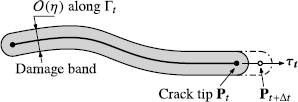
Damage band structuration along a pre-defined path \(l\mapsto \boldsymbol{\gamma}(l)\) indicating a crack propagating in the direction of \(\boldsymbol{\tau}_{t}\) with its tip located at \(\mathbf{P}_{t}\)
-
2.
During propagation the damage profile along this curve \(l\mapsto \boldsymbol{\gamma}(l)\) develops a cross-section of the same order of \(\eta\). The current damage evolution rate \(\dot{\alpha}_{t}\) is partitioned into two components: one that contributes to crack advance in the propagation direction, and the other that describes possible profile evolution in the coordinate system that moves with the crack tip \(\mathbf{P}_{t}\). Formally, we make use of the diffeomorphism \(\boldsymbol{\phi}\) introduced in Sect. 2.1 that transforms the current cracked configuration to the initial one, in the context of gradient damage models where cracks refer to the totally damaged curve (43). The evolution of the damage field \(\alpha_{t}\) is thus given by
$$ \alpha_{t}\circ\boldsymbol{\phi}=\alpha_{t}^{*}, $$(44)where the damage profile field \(\alpha_{t}^{*}\) corresponds to an initial crack which remains stationary
$$\bigl\{ \mathbf{x}\in\varOmega\bigm|\alpha_{t}^{*}(\mathbf{x})=1 \bigr\} = \varGamma_{0}. $$The establishment of such initial damage field which corresponds to \(\varGamma_{0}\) is beyond the scope of this paper. Using the classical chain rule, the time derivative of the damage reads
$$ \dot{\alpha}_{t}(\mathbf{x})=\dot{\alpha}_{t}^{*} \bigl(\mathbf{x}^{*} \bigr)-\dot{l}_{t}\nabla\alpha_{t}( \mathbf{x})\cdot\boldsymbol{\theta}_{t}(\mathbf{x}), $$(45)which reflects faithfully our partition of the damage rate. Remark that if the crack is arrested \(\dot{l}_{t}=0\), the total damage rate corresponds to that of the profile evolution.

Remark 4
Hypothesis 1 highlights the scope of the current contribution: propagation (or arrest) of an initially existing phase-field crack (damage band), without complex topology changes such as kinking or branching. For illustration purposes, several situations are presented in Fig. 8.
-
(a)
The current paper focuses on the further propagation of an existing damage band as illustrated in Fig. 8(a).
Fig. 8 
Illustrations of the scope of the present paper: (a) a simple phase-field crack with its tip \(\mathbf{P}_{t}\), (b) a discrete crack in the domain with an identically zero damage field \(\alpha_{t}=0\) and (c) a phase-field crack at branching, leading to the existence of two crack tips (same as in Fig. 5). The damage field varies from 0 (blue zones) to 1 (red zones). The current paper focuses on (a), and studies further propagation of the existing phase-field crack (Color figure online)
-
(b)
Discrete cracks as a geometric discontinuity in the domain are not to be confused with phase-field like cracks (damage band). The current paper does not consider the further “propagation” of the tip \(\mathbf{P}_{t}\) appearing in Fig. 8(b), since the damage field is identically zero \(\alpha_{t}=0\). The determination of an initial damage field in such cracked domain refers to the phase-field crack nucleation problem, and is subject to the irreversibility condition, the damage criterion (40) and the consistency condition (42).
-
(c)
Complex topology changes in the damage band illustrated in Fig. 5 and Fig. 8(c) are not considered in this paper.

Furthermore, the crack path, straight or curved, is assumed to be pre-defined. Crack path prediction is indeed the raison d’être of phase-field models of fracture, see for example [6, 17]. A thorough investigation of this point is a very important task to which future work will be devoted. Nevertheless, the current contribution focuses on the behavior of gradient damage models when the crack path is not of concern, which permits a direct comparison with the classical Griffith’s theory of dynamic fracture without additional hypotheses, i.e., Griffith’s law (22). We concentrate on “when” cracks propagate (temporal evolution) and not on “how” cracks propagate (spatial evolution).
From (44), the current damage field \(\alpha_{t}\) can be considered as a function depending on the current crack length \(l_{t}\) and the current damage profile \(\alpha_{t}^{*}\). Using the diffeomorphism we can thus rewrite the space-time action integral (34) in the initial cracked configuration \({\varOmega\setminus \varGamma_{0}}\), by transforming the displacement via (6). Since we assume that the crack \(\varGamma_{t}\) (or the totally damaged zone) is of measure zero with respect to \(\mathrm{d}\mathbf{x}\) (and hence also to \(\mathrm{d}\mathbf{x}^{*}\)), contribution on this subset \(\varGamma_{t}\) can be neglected. The damage-dependent elastic energy (29) is then given by
and the non-local damage dissipation energy now reads
where the identity \(\nabla\alpha_{t}(\mathbf{x})=\nabla\boldsymbol {\phi }^{-\mathsf{T}}(\mathbf{x}^{*})\nabla\alpha_{t}^{*}(\mathbf{x}^{*})\) is used following (44). The kinetic energy and the external work potential are still formally given by (10) and (11) since damage is not involved in these two functionals. The generalized space-time action integral (34) is hence given by
The definition of the admissible evolution spaces for the triplet \((\mathbf{u}^{*},\alpha^{*},l)\) are discussed as follows. The same admissible function spaces for the displacement (12) and for the crack length evolution (13) defined in the sharp-interface fracture model can be used as long as we interpret the crack \(\varGamma_{t}\) as the totally damaged curve (43). The damage profile \(\alpha ^{*}\) is merely a component contributing to the total damage evolution, hence the temporal irreversibility still applies to the true damage evolution \(t\mapsto\alpha_{t}\), which reads \(\dot{\alpha}_{t}\geq0\). Given an arbitrary such evolution verifying Hypothesis 1, we want to consider admissible variation of the current damage state \(\alpha_{t}\) corresponding to a crack length \(l_{t}\), based on an admissible crack length variation \(\delta l_{t}=s_{t}-l_{t}\geq0\) and a crack profile variation \(\beta_{t}^{*}-\alpha_{t}^{*}\). At time \(t\in(0,T)\) the induced admissible non-negative variation of the true damage reads
As can be seen, the damage profile variation \(\beta_{t}^{*}-\alpha_{t}^{*}\) and the crack length variation \(\delta l_{t}\) are now involved in a unilateral fashion to ensure irreversibility of the true damage:
-
If the crack length variation is zero \(\delta l_{t}=0\), then the damage profile variation \(\beta_{t}^{*}-\alpha_{t}^{*}\) corresponds exactly to the true damage variation \(\beta_{t}-\alpha_{t}\). Thus it suffices that \(\beta_{t}^{*}-\alpha_{t}^{*}\geq0\) to ensure irreversibility.
-
However if a finite extension of the crack length is considered \(\delta l_{t}>0\), then the damage profile variation depends non-trivially on the \(\delta l_{t}\) via (49) to obtain \(\beta _{t}-\alpha _{t}\geq0\).
In practice, it means that if crack length variation is not considered, then the variation of the action integral with respect to the displacement and to the damage (profile) can be separately computed. Otherwise when \(\delta l_{t}>0\), then damage variation must also be taken into account. Given an admissible crack length evolution \(s\in\mathcal {Z}(l)\), the admissible evolution space for the damage profile will be denoted by \(\mathcal{D}_{s}(\alpha^{*})\), where the dependence on \(s\) is explicitly indicated by the subscript and \(\alpha^{*}\) describes the profile of a damage evolution verifying Hypothesis 1. As usual, at both ends of the time interval \(I\), no variations of true damage profile are considered.
Associated with an admissible triplet of displacement, damage profile and crack length evolutions \((\mathbf{u}^{*},\alpha^{*},l)\in\mathcal {C}(\mathbf{u}^{*})\times\mathcal{D}_{l}(\alpha^{*})\times\mathcal {Z}(l)\), we can now reformulate the dynamic gradient damage model under Hypothesis 1 by the following
Definition 4
(Dynamic gradient damage evolution law for a propagating crack)
-
1.
Irreversibility: the damage \(t\mapsto\alpha_{t}\) and the crack length \(t\mapsto l_{t}\) are non-decreasing functions of time.
-
2.
First-order stability: the first-order action variation is non-negative with respect to arbitrary admissible displacement, damage profile and crack evolutions
$$\begin{aligned} &\mathrm{A}' \bigl(\mathbf{u}^{*},\alpha^{*},l \bigr) \bigl(\mathbf{v}^{*}-\mathbf{u}^{*},\beta^{*}-\alpha^{*},s-l \bigr)\geq 0 \\ &\quad\text{for all } \mathbf{v}^{*}\in\mathcal{C} \bigl(\mathbf{u}^{*} \bigr),\mbox{ all }\beta ^{*}\in \mathcal{D}_{s} \bigl(\alpha^{*} \bigr)\mbox{ and all }s\in\mathcal{Z}(l). \end{aligned}$$(50) -
3.
Energy balance: the only energy dissipation is due to crack propagation such that we have the following energy balance
$$ \mathcal{H}_{t}=\mathcal{H}_{0}+ \int_{0}^{t} \biggl( \int_{\varOmega\setminus \varGamma _{s}} \bigl(\boldsymbol{\sigma}_{s}\cdot \boldsymbol{\varepsilon}(\dot{\mathbf{U}}_{s})+\rho\ddot{ \mathbf{u}}_{s}\cdot\dot{\mathbf{U}}_{s} \bigr)\,\mathrm{d} \mathbf{x}-\mathcal{W}_{s}(\dot{\mathbf{U}}_{s})-\dot{ \mathcal{W}}_{s}(\mathbf{u}_{s}) \biggr)\,\mathrm{d}s, $$(51)where the total energy is defined by
$$ \mathcal{H}_{t}=\mathcal{E}^{*} \bigl(\mathbf{u}_{t}^{*}, \alpha_{t}^{*},l_{t} \bigr)+\mathcal{S}^{*} \bigl( \alpha_{t}^{*},l_{t} \bigr)+\mathcal{K} \bigl( \mathbf{u}_{t}^{*},\dot{\mathbf{u}}_{t}^{*},l_{t},\dot {l}_{t} \bigr)-\mathcal{W}_{t}^{*} \bigl(\mathbf{u}_{t}^{*},l_{t} \bigr). $$(52)
We then exploit the first-order stability condition (50) by carefully developing the Gâteaux derivative of the action integral (48). With the help of detailed calculations provided in Appendix A and using the same arguments developed before, the first-order action variation testing with \(\beta ^{*}-\alpha^{*}=0\) and \(s-l=0\) leads to the elastic-damage dynamic wave equation on the uncracked domain similar to (19) and (38)
where we recall that here the stress tensor \(\boldsymbol{\sigma}_{t}\) is damage-dependent. Similarly at fixed displacement and crack length variations, evaluating the directional derivative of the action integral with respect to damage variation \(\beta^{*}-\alpha^{*}\) leads to
where the integration domain is first transformed to the current cracked one and an integration by parts is then performed. Since the induced true damage variation is non-negative due to (49), we obtain thus the same local damage criterion (40) as before. Finally, we consider the first-order action variation with respect to crack length evolution variation. Through (49), damage profile variation is thus coupled with that of the crack length. We thus merely have
with a generalized dynamic energy release rate defined by
This quantity contains the conventional dynamic energy release rate (note that compared to (21), here the elastic energy and the stress tensor depends on the damage state)
and the damage dissipation rate as the partial derivative of the damage dissipation energy \(\mathcal{S}^{*}(\alpha_{t}^{*},l_{t})\) with respect to the crack length
In (54), although the crack length variation is non-negative \(\delta l_{t}\geq0\), the sign of the generalized dynamic energy release rate is undetermined in general, since the first two terms are both positive due to (40) and (49).
It remains to use the energy balance (51) to derive the consistency conditions. With the help of calculations given in Appendix B, we obtain
where the first term represents energy dissipation due to damage profile evolution following (45) and the second term corresponds to damage dissipation on the uncracked boundary where \(\boldsymbol{\theta}_{t}=\mathbf{0}\). The third term denotes dissipation due to pure propagation of the phase-field crack. It can be observed that in case of a currently stationary crack \(\dot{l}_{t}=0\), we retrieve directly the classical consistency conditions for damage (42). However when the crack propagates \(\dot{l}_{t}>0\), nothing can be deduced from (58) since the damage profile evolution \(\alpha^{*}\) is not necessarily irreversible and the sign of \(\widehat {G}_{t}\) is not yet known.
From Proposition 1, the dynamic energy release rate (21) in the Griffith’s theory of fracture can be written as a path integral. This property can be extended to the dynamic gradient damage model due to the analogies with their respective variational ingredients.
Proposition 2
The generalized dynamic energy release rate (55) defines a generalized \(\widehat{J}\)-integral
where the generalized dynamic \(\widehat{\mathbf{J}}_{t}\) tensor is defined by
As in Proposition 1, here \(\mathbf{n}\) denotes the normal pointing out of the ball \(B_{r}(\mathbf{P}_{t})\) with \(C_{r}=\partial B_{r}(\mathbf{P}_{t})\) its boundary.
Proof
Equation (59) can be obtained mainly by following the proof of Proposition 1. The last term containing the damage gradient results from the identity below which accounts for the damage dependence of the elastic energy and the damage dissipation energy
together with an additional integration by parts
To pass from the Lagrangian density in (55) to the Hamiltonian density in (60), it suffices to observe that the most singular part of the time derivatives corresponds to the transport term. Similar calculations at the end of the proof of Proposition 1 then lead to the desired result. □
The tensor \(\widehat{\mathbf{J}}_{t}\) can be seen as the dynamic extension of the quasi-static generalized Eshelby tensor (or energy-momentum tensor) introduced respectively in the quasi-static gradient damage model [29] and the dissipative phase field model originating from the physics community, see for instance [5, 13]. Inserting (59) into (58), an equivalent expression of the consistency condition can be obtained
In [29], a careful singularity analysis is conducted to determine the sign of the \(\widehat{J}\)-integral with a particular strongly brittle material. Such calculations could be extended to the dynamic setting but are beyond the scope of this paper. Based on numerical verifications, we assume the following:
Hypothesis 2
The generalized dynamic \(\widehat{J}\)-integral is non-positive
for all damage constitutive laws \(\alpha\mapsto\mathsf{A}(\alpha)\) and \(\alpha\mapsto w(\alpha)\) which characterize the behavior of a strongly brittle material.
Due to the local damage criterion (40) and the irreversibility conditions, each term in (62) is non-positive while their sum yields zero, which implies that each term vanishes separately
which represent local energy balances. We note that the first two equalities correspond to the consistency condition (42) derived without Hypothesis 1.
It can be seen from (63) and the last equation in (64) that the generalized dynamic \(\widehat{J}\)-integral plays the role of \(G_{t}-G_{\mathrm{c}}\) in the classical Griffith’s law (22). It involves a path integral on a contour \(C_{r}\) that shrinks to the crack tip \(r\to0\), which may lead to difficulties in a finite element calculation. From a numerical point of view, the generalized dynamic energy release rate \(\widehat{G}_{t}\) defined in (55) should be preferred since it is written as a cell integral on a finite domain. It turns out that under a particular circumstance, these two objects are equivalent and they both define the following generalized Griffith criterion.
Proposition 3
(Generalized Griffith criterion)
The crack tip equation of motion predicted by the dynamic gradient damage model is governed by the following generalized Griffith criterion:
If we assume that in (45) the time derivative of the damage profile is negligible compared to the transport term and furthermore the damage gradient in the direction of crack propagation is non-positive at every time \(t\) and almost everywhere
then the generalized dynamic energy release rate (55) can be equivalently used in the above generalized Griffith criterion, which leads to
Proof
Using the definition of \(\widehat{J}_{t}\) in (59) and the second condition in (66), we obtain the equivalent stability condition
since \(Y_{t}+\operatorname{div}\mathbf{q}_{t}\leq0\) due to the local damage criterion (40). If the first condition in (66) holds, then the local consistency condition for damage in (58) reads
Multiplying (59) by \(\dot{l}_{t}\) gives the desired condition \(\widehat{G}_{t}\dot{l}_{t}=0\). □
Remark 5
These two conditions (66) needed to establish (67) can be justified in the crack tip problem when the internal length is small compared to the dimension of the body.
Remark 6
Proposition 3 and in particular (65) and (67) constitute one of the main results of the present contribution. Above all, arbitrary damage evolution in the dynamic gradient damage model is governed by the irreversibility condition, the damage criterion (40) and the consistency condition (42). However it is shown that the propagation (or arrest) of an existing damage band (phase-field crack) is governed by the above Griffith like scalar equations involving several energy release rate concepts.
4 Separation of Scales and Asymptotic Griffith’s Law
We remind the reader that the generalized dynamic \(\widehat{J}\)-integral as well as the generalized dynamic energy release rate \(\widehat{G}_{t}\) that enter into the generalized Griffith’s law (Proposition 3) don’t possess directly an intuitive interpretation in fracture mechanics terminology. To establish the link between damage and fracture, we will essentially follow the separation of scales made in the quasi-static case [29] (and similar in essence to that reviewed in [13]) which decomposes the complete gradient damage evolution problem into three subproblems, see Fig. 9. From now on, all quantities that depend on the internal length will be indicated by a superscript \(\eta\). We also adopt the assumption made on the internal length dependence of the external loading, namely

Separation of scales conducted in [29] which decomposes the gradient damage evolution problem into three sub-problems: the outer linear elastic fracture mechanics problem where the damage band is replaced by a true crack in the domain, the damage band problem in which the fracture toughness can be identified with the energy dissipated during the damage band creation and the crack tip problem where the matching conditions with the previous two subproblems will be used
4.1 Outer Linear Elastic Dynamic Fracture Problem
Due to the linear nature of the macroscopic dynamic fracture problem on the cracked domain \({\varOmega\setminus\varGamma_{t}}\), dependence of the real mechanical fields on the internal length can be given by
In linear elastic fracture mechanics, the displacement and stress present a well-known \(\mathcal{O}(r^{1/2})\) and \(\mathcal{O}(r^{-1/2})\) asymptotic behaviors and in the case of an in-plane fracture problem they admit the following near-tip form
where compared to the quasi-static regime the angular functions \(\boldsymbol{\varTheta}\)’s and \(\boldsymbol{\varSigma}\)’s depend on the current crack speed [11]. When the crack propagates \(\dot{l}_{t}>0\), the near tip behaviors for the velocity and the acceleration fields develop the following steady state form:
In particular, the asymptotic expansion of the velocity reads
An equivalent dynamic energy release rate associated with this outer problem can then be defined using Proposition 1 and the asymptotic near-tip behavior of the fields (70) and (72), which under the plane strain condition results in
where \(A\)’s are again two universal material-dependent functions, see [11, p. 234]. Due to (69), (70) and (73), the energy release rate \(G_{t}^{\eta}\) is of order \(\mathcal{O}(\eta)\) while the stress intensity factors \(K^{\eta}\)’s are of order \(\mathcal{O}(\sqrt{\eta})\), i.e.,
where \(\overline{G}_{t}\) and \(\overline{K}\)’s are respectively the rescaled equivalent dynamic energy release rate and the rescaled stress intensity factors.
4.2 Damage Band Problem
The damage band problem will be essentially the same as in the quasi-static case [29], due to the formally identical energy minimization principle (39) and its local interpretations (40) and (42). The first-order term of the damage field \(\alpha _{t}^{\eta}\) inside or near the crack band but far from the crack tip admits the following form
where \(\alpha_{*}\) is the normalized (with respect to \(\eta\)) damage profile along the crack normal at a certain arclength \(s\) of the crack \(\varGamma_{t}\) and \(\operatorname{dist}(\mathbf{x},\varGamma_{t})\) is the Euclidean distance from the point \(\mathbf{x}\) near the crack band to the crack \(\varGamma_{t}\). The damage gradient in the tangential direction is thus negligible compared to that in the normal direction
Using the definition of the dual quantities (41), the consistency condition (42) during the crack band creation reads
Note that in this damage band problem the term \(\frac{1}{2}\mathsf {A}'(\alpha_{*})\boldsymbol{\varepsilon}(\mathbf{u}_{t}^{\eta})\cdot \boldsymbol{\varepsilon}(\mathbf{u}_{t}^{\eta})\) is still of order \(\mathcal{O}(\eta)\) due to (69) while the other two terms in (77) are of order \(\mathcal {O}(1)\), which leads to the following first-order damage profile condition:
One can easily solve this autonomous second order differential equation within the normalized damage band \([-\overline{D},\overline{D}]\) by using the boundary conditions of \(\alpha_{*}\) and the reader are referred to [29] for a detailed derivation. The energy per unit length dissipated during the damage band creation can be calculated by the integral of the damage dissipation density (31) over the real cross section \([-\eta\overline{D},\eta \overline{D}]\), which gives
This energy as in the quasi-static case [29] will play the role of the fracture toughness in the asymptotic Griffith’s law.
4.3 Crack Tip Problem
We perform the same translation and rescaling of the system of coordinates \(\mathbf{y}=(\mathbf{x}-\mathbf{P}_{t})/\eta\) in the vicinity of the crack tip and assume the following near-tip forms of the displacement, stress and damage fields established in Sect. 3.3 of [29]:
with \(\mathbf{u}_{t}(\mathbf{P}_{t})\) the displacement of the crack tip given by the outer problem (69) and \(\overline{\boldsymbol {\sigma}}_{t}=\mathsf{A}(\overline{\alpha}_{t})\boldsymbol{\varepsilon }(\overline{\mathbf{u}}_{t})\). In dynamics, the asymptotic expansion of the velocity \(\dot{\mathbf{u}}_{t}^{\eta}\) and the acceleration \(\ddot{\mathbf{u}}_{t}^{\eta}\) can be obtained by differentiating \(\mathbf{u}_{t}^{\eta}\) with respect to time, which gives to their first order with respect to the internal length
These equations illustrate in fact the steady-state condition (71) for the crack tip problem. We note that here the stress, the velocity and the acceleration are of order \(\mathcal {O}(1)\) while they are of order \(\mathcal{O}(\sqrt{\eta})\) in the outer problem. Using the expressions (70) and (72), the behavior of \(\overline{\boldsymbol{\sigma}}_{t}\) and \(\dot {\mathbf{u}}_{t}\) far from the crack tip can thus be obtained by virtue of the following matching conditions
Since the body force density \(\mathbf{f}_{t}^{\eta}\) is of higher order, the first-order dynamic equilibrium for this crack tip problem reads
where \(\overline{\varGamma}=(-\infty,0)\times \{0 \}\) corresponds to a rescaled crack along the direction \(\mathbf{e}_{1}\), where \(\overline {\alpha}_{t}=1\).
We now turn to damage evolution in the crack tip problem. In the rescaled coordinate system the virtual perturbation admits the form \(\boldsymbol{\theta}_{t}(\mathbf{y})=\theta_{t}(\mathbf{y})\mathbf {e}_{1}\) where \(0\leq \theta _{t}(\mathbf{y})\leq1\). From the chain rule, the rate of damage (45) is of order \(\mathcal{O}(1/\eta)\) and reads
where the damage profile rate disappears since it is of higher order. This corresponds to the first condition assumed in (66). Due to the irreversibility condition of damage, when the crack propagates \(\dot{l}_{t}>0\) the term \(\nabla \overline{\alpha}_{t}(\mathbf{y})\cdot\boldsymbol{\theta}_{t}(\mathbf {y})\) is necessarily non-positive. We assume that the condition remains true at every time. It is sufficient that the damage remains constant near the crack tip when the crack is arrested.
Hypothesis 3
We assume that \(\nabla\alpha_{t}\cdot\boldsymbol{\theta}_{t}\leq0\) for every time.
This corresponds to the second condition of (66). All the terms in the local damage criterion (40) are of order \(\mathcal {O}(1)\), hence at the first order we have
The damage field \(\overline{\alpha}_{t}\) should also be matched to its asymptotic expansions for the outer and the damage band problems, which implies
Since all conditions in (66) are satisfied in the crack tip problem, the generalized Griffith criterion admits the form (67) involving the above two objects. We will take advantage of the asymptotic behavior of the fields (81) and (85) to analyze that of the conventional dynamic energy release rate (56) and the damage dissipation rate (57). Note that they are both of order \(\mathcal{O}(\eta)\) as in the case for \(G_{t}^{\eta}\) in (74) as well as for \(G_{\mathrm{c}}^{\eta}\) in (79), and thus are rescaled accordingly
Proposition 4
Using virtual perturbations defined in Fig. 10, the damage dissipation rate (57) converges to the fracture toughness (79) defined in the damage band problem in the limit \(r\to\infty\).

A particular virtual perturbation \(\boldsymbol{\theta}_{t}\) in the scaled coordinate system \(\mathbf{y}=(\mathbf{x}-\mathbf{P}_{t})/\eta\) adapted from Fig. 2
Proof
Within the scaled coordinate system we will construct a particular family of virtual perturbations of form \(\boldsymbol{\theta }_{t}(\mathbf{y})=\theta _{t}(\mathbf{y})\mathbf{e}_{1}\) as illustrated in Fig. 10. As can be seen, the definition is adapted from Fig. 2. The asymptotic behavior of the rescaled damage dissipation rate \(\overline {\gamma}_{t}\) is analyzed when the inner radius \(r\) goes to infinity with a fixed ratio of \(R/r\). As \(\nabla\theta_{t}=\mathbf{0}\) inside \(B_{r}(\mathbf{P}_{t})\), the scaled damage dissipation rate \(\overline {\gamma}_{t}\) reads
where the integral is defined on the uncracked crown by \(\circledcirc _{r}= (B_{R}(\mathbf{P}_{t})\setminus B_{r}(\mathbf{P}_{t}) )\setminus \varGamma_{t}\) and \(\overline{\varsigma}\) is the rescaled damage dissipation energy given by
Integrating by parts the virtual perturbation gradient term and using (61), we obtain
where the boundary integral is due to the fact that \(\boldsymbol {\theta }_{t}=\mathbf{e}_{1}\neq\mathbf{0}\) only on the inner circle \(C_{r}=\partial B_{r}(\mathbf{P}_{t})\) and \(\boldsymbol{\theta}_{t}\cdot \mathbf{n}=0\) on \(\varGamma_{t}\). Note that here the vector \(\mathbf{n}\) is defined as the normal pointing into the circle \(C_{r}\) and \(\mathrm{d}\mathbf{a}\) denotes the arc length measure associated with \(\mathrm{d}\mathbf{y}\). From the damage band problem we have \(\nabla \overline {\alpha}_{t}\cdot\mathbf{e}_{1}=0\) away from the crack tip \(\mathbf {P}_{t}\), see (76). Hence using the matching condition with the damage band problem (85) we have in the limit \(r\to \infty\)
where the last equality comes from the definition of \(\overline {G}_{\mathrm{c}}\) in (79). □
Proposition 5
Using virtual perturbations defined in Fig. 10, the conventional dynamic energy release rate (56) converges to the equivalent dynamic energy release rate of the outer problem (73) in the limit \(r\to\infty\).
Proof
The conventional dynamic energy release rate will still be calculated with the above introduced virtual perturbation of Fig. 10. The term involving the body force density in (56) will be neglected since it is of higher order. By denoting the uncracked inner ball by \(\tilde{B}_{r}=B_{r}(\mathbf{P}_{t})\setminus\varGamma_{t}\), we will partition \(\overline{G}^{\alpha}_{t}\) defined on \(B_{R}(\mathbf {P}_{t})\setminus \varGamma_{t}\) into two parts
where we note that the virtual perturbation \(\boldsymbol{\theta}_{t}\) is constant and is equal to the crack propagation direction \(\mathbf{e}_{1}\) inside \(B_{r}(\mathbf{P}_{t})\) by definition. Using the identities and integrations by parts similar to (24), (25) and (61), the first part defined in the crown \(\circledcirc _{r}\) can be written as
where the integral on the circle \(C_{r}=\partial B_{r}(\mathbf{P}_{t})\) comes from the integration by parts of the term \(\boldsymbol{\sigma} (\boldsymbol{\varepsilon}(\overline{\mathbf{u}}_{t}),\overline {\alpha}_{t} )\cdot(\nabla\overline{\mathbf{u}}_{t}\nabla \boldsymbol{\theta}_{t})\), the boundary conditions of \(\boldsymbol {\theta}_{t}\) due to definition, and the fact that \(\mathbf{n}\) is defined as the normal pointing out of the ball \(\partial B_{r}(\mathbf{P}_{t})\). Thanks to dynamic equilibrium (82), we have
where the second equality follows by the integration by parts of the divergence term with the same remarks about the normal and the boundary conditions of \(\boldsymbol{\theta}_{t}\).
Using the steady state condition (80) for this crack tip problem and the integration by parts similar to (27), the second part of (87) reads
because \(\operatorname{div}\boldsymbol{\theta}_{t}=0\) inside the inner ball \(B_{r}(\mathbf{P}_{t})\). Regrouping \((\overline{G}^{\alpha}_{t} )_{1}\) and \((\overline {G}^{\alpha}_{t} )_{2}\), we obtain thus
When the inner radius \(r\) tends to infinity, we observe that the angular sector corresponding to \(\overline{\alpha}_{t}>0\) goes to zero. Using the matching conditions of the mechanical fields (81) and of the damage field (85) which implies that \(\nabla\overline{\alpha}_{t}\cdot\mathbf{e}_{1}\to0\), see (76), we obtain in this limit
where \(\overline{\mathbf{J}}_{t}\) is the rescaled dynamic \(\mathbf{J}\) tensor (23) corresponding to the outer problem and the last equality comes from Proposition 1 and (74). □
Proposition 6
(Asymptotic Griffith’s law)
The crack tip evolution in the dynamic gradient damage model is governed by the following asymptotic Griffith’s law as long as the material internal length is sufficiently small compared to the dimension of the body:
Proof
Irreversibility follows directly by the generalized Griffith criterion (67). Using its definition (55) and the rescaling condition (86), the generalized dynamic energy release rate reads
Thanks to the two asymptotic results from Propositions 4 and 5 and the rescaling conditions (74) and (79), the desired crack stability and energy balance conditions can be obtained by passing the limit \(r\to\infty\) using virtual perturbations defined in Fig. 10. □
Remark 7
Proposition 6 constitutes another main result of the present paper. It can be regarded as an asymptotic interpretation of Proposition 3. When the internal length is small, it is shown that the propagation of a phase-field like crack is driven by the dynamic energy release rate of the outer mechanical response. Numerical verification of this asymptotic Griffith’s law is performed in [18] for a mode-III crack propagation situation.
Remark 8
Based on a generalized energy-momentum tensor in the quasi-static phase-field model of fracture, authors of [5, 13] also established a link between the phase-field crack evolution and classical Griffith’s theory, by providing an equivalent energy release rate. The separation of scales considered here summarizes and justifies the asymptotic behaviors of the displacement and damage fields assumed in their analyses.
5 Conclusion and Perspectives
In the formulation of dynamic gradient damage models, inertia effects are taken into account solely via an inclusion of the kinetic energy into the space-time action integral. Static equilibrium is thus replaced by an elastic-damage wave equation (38), however the same energy minimization principle (39) still governs the damage evolution as in the quasi-static model. Nevertheless it turns out that the crack tip equation of motion becomes automatically rate-dependent and follows a dynamic evolution law (Proposition 3 and Proposition 6), thanks to the definition of the generalized dynamic \(\widehat{J}\)-integral and the generalized dynamic energy release rate \(\widehat{G}_{t}\). The attentive reader can not fail to realize the essential role played by the variational nature of the formulation in the derivation of these concepts, which is applicable for a large class of damage constitutive laws. Using the three physical principles of irreversibility, stability and energy balance, analogies between different models can be rigorously formalized. Properties derived in one model can be translated to the others, which is the case observed for the variational dynamic fracture model and the dynamic gradient damage model during the crack propagation phase, see Table 1. In particular, the equation of motion governing the crack tip can be obtained by calculating the first-order action variation with respect to arbitrary crack evolution and by using the energy balance condition. This procedure could be repeated for other variational formulations of crack evolutions. An interesting extension would be the gradient damage model coupled with plasticity [3].
Another novelty of this contribution concerns the application of shape derivative methods [9] to the gradient damage model. Thanks to a well-defined diffeomorphism, in the sharp-interface fracture model the current cracked material configuration on which mechanical quantities are defined is transformed to the initial cracked one. Similarly in the phase-field approach the current damage field representing a propagating crack is mapped from a damage profile field which corresponds to a stationary initial crack. This Lagrangian formalism gives a rigorous sense to the Gâteaux derivative of the action integral with respect to the current crack length, which leads in return to the definition of an energy release rate even in the absence of stress singularities.
The most essential assumption behind the generalized Griffith criterion resides in the non-positivity of the generalized \(J\)-integral. A theoretic proof of Hypothesis 2 calls for a careful singularity analysis similar to that conducted in [29]. Let’s recall that the crack topology is restricted in this paper to a single straight line. Following the discussion at the end of Sect. 2, predefined curved crack paths can as well be considered. When several cracks are present in the body, as long as a diffeomorphism similar to (5) can be constructed between the initial cracked configuration and a perturbed multi-cracked configuration (generally speaking when those cracks do not interact with each other), the formalism described in this paper can still be applied. By relaxing furthermore the hypothesis of a pre-defined crack propagation path, we may hope to identify a macroscopic kinking/branching criterion hidden behind the stability condition (35). An interesting challenge would be to use more adequate shape derivative methods [15] in order to differentiate the action integral with respect to the propagation angle. Furthermore we assume that the totally damaged zone corresponds to a subset of measure zero with respect to \(\mathrm{d}\mathbf{x}\). When it is not the case, more energy would be dissipated during crack propagation which could represent an increase of the apparent fracture toughness observed during dynamic crack microbranching processes [28]. Finally, only the crack propagation phase of an existing damage band (phase-field crack) is considered in this paper. The establishment of an initial damage field in a body with possible geometric defects is subject to the irreversibility condition, the damage criterion (40) and the consistency condition (42). The generalized Griffith criterion stated in Proposition 3 and the asymptotic Griffith’s law stated in Proposition 6 no longer apply in this situation since an initial phase-field crack is absent and a separation of scales is not possible. It refers to the dynamic phase-field crack nucleation problem to which future work will be devoted.
Notes
But in practice it is the initial displacement \(\mathbf{u}_{0}\) and velocity \(\dot{\mathbf{u}}_{0}\) that are known and we will use the equations derived from the Hamiltonian principle to solve the physical Initial Value Problem.
References
Abdelmoula, R., Debruyne, G.: Modal analysis of the dynamic crack growth and arrest in a DCB specimen. Int. J. Fract. 188(2), 187–202 (2014)
Adda-Bedia, M., Arias, R., Amar, M.B., Lund, F.: Generalized Griffith criterion for dynamic fracture and the stability of crack motion at high velocities. Phys. Rev. E 60(2), 2366–2376 (1999)
Alessi, R., Marigo, J.J., Vidoli, S.: Gradient damage models coupled with plasticity: variational formulation and main properties. Mech. Mater. 80, 351–367 (2015)
Attigui, M., Petit, C.: Numerical path independent integral in dynamic fracture mechanics. In: ECF 11—Mechanisms and Mechanics of Damage and Failure (1996)
Ballarini, R., Royer-Carfagni, G.: Closed-path J-integral analysis of bridged and phase-field cracks. J. Appl. Mech. 83(6), 061,008 (2016)
Borden, M.J., Verhoosel, C.V., Scott, M.A., Hughes, T.J., Landis, C.M.: A phase-field description of dynamic brittle fracture. Comput. Methods Appl. Mech. Eng. 217–220, 77–95 (2012). doi:10.1016/j.cma.2012.01.008
Bourdin, B., Francfort, G.A., Marigo, J.J.: The variational approach to fracture. J. Elast. 91(1–3), 5–148 (2008)
Bourdin, B., Larsen, C.J., Richardson, C.L.: A time-discrete model for dynamic fracture based on crack regularization. Int. J. Fract. 168(2), 133–143 (2011)
Destuynder, P., Djaoua, M.: Sur une interprétation mathématique de l’intégrale de Rice en théorie de la rupture fragile. Math. Methods Appl. Sci. 3(1), 70–87 (1981)
Freddi, F., Royer-Carfagni, G.: Regularized variational theories of fracture: a unified approach. J. Mech. Phys. Solids 58(8), 1154–1174 (2010). doi:10.1016/j.jmps.2010.02.010
Freund, L.B.: Dynamic Fracture Mechanics. Cambridge University Press, Cambridge (1990). doi:10.1017/CBO9780511546761
Griffith, A.A.: The phenomena of rupture and flow in solids. Philos. Trans. R. Soc. Lond. 221, 163–198 (1921)
Hakim, V., Karma, A.: Laws of crack motion and phase-field models of fracture. J. Mech. Phys. Solids 57(2), 342–368 (2009). doi:10.1016/j.jmps.2008.10.012
Hamilton, W.R.: On a general method in dynamics. Philos. Trans. R. Soc. Lond. 124, 247–308 (1834)
Hintermüller, M., Kovtunenko, V.A.: From shape variation to topological changes in constrained minimization: a velocity method-based concept. Optim. Methods Softw. 26(4–5), 513–532 (2011)
Khludnev, A., Sokołowski, J., Szulc, K.: Shape and topological sensitivity analysis in domains with cracks. Appl. Math. 55(6), 433–469 (2010)
Li, T., Marigo, J.J., Guilbaud, D., Potapov, S.: Gradient damage modeling of brittle fracture in an explicit dynamics context. Int. J. Numer. Methods Eng. (2016). doi:10.1002/nme.5262
Li, T., Marigo, J.J., Guilbaud, D., Potapov, S.: Numerical investigation of dynamic brittle fracture via gradient damage models. Adv. Model. Simul. Eng. Sci. 3, 26 (2016). doi:10.1186/s40323-016-0080-x
Lorentz, E., Andrieux, S.: A variational formulation for nonlocal damage models. Int. J. Plast. 15(2), 119–138 (1999). doi:10.1016/S0749-6419(98)00057-6
Lorentz, E., Godard, V.: Gradient damage models: toward full-scale computations. Comput. Methods Appl. Mech. Eng. 200(21–22), 1927–1944 (2011). doi:10.1016/j.cma.2010.06.025
Maugin, G.: On the \(J\)-integral and energy-release rates in dynamical fracture. Acta Mech. 105(1–4), 33–47 (1994). doi:10.1007/BF01183940
Nishioka, T., Atluri, S.N.: Path-independent integrals, energy release rates, and general solutions of near-tip fields in mixed-mode dynamic fracture mechanics. Eng. Fract. Mech. 18(1), 1–22 (1983)
Oleaga, G.E.: Remarks on a basic law for dynamic crack propagation. J. Mech. Phys. Solids 49(10), 2273–2306 (2001)
Pham, K., Amor, H., Marigo, J.J., Maurini, C.: Gradient damage models and their use to approximate brittle fracture. Int. J. Damage Mech. 20(4), 618–652 (2011)
Pham, K., Marigo, J.J.: Approche variationnelle de l’endommagement: II. Les modèles à gradient. C. R., Méc. 338(4), 199–206 (2010)
Pham, K., Marigo, J.J.: From the onset of damage to rupture: construction of responses with damage localization for a general class of gradient damage models. Contin. Mech. Thermodyn. 25(2–4), 147–171 (2013)
Pham, K., Marigo, J.J., Maurini, C.: The issues of the uniqueness and the stability of the homogeneous response in uniaxial tests with gradient damage models. J. Mech. Phys. Solids 59(6), 1163–1190 (2011)
Sharon, E., Fineberg, J.: Microbranching instability and the dynamic fracture of brittle materials. Phys. Rev. B 54, 7128–7139 (1996). doi:10.1103/PhysRevB.54.7128
Sicsic, P., Marigo, J.J.: From gradient damage laws to Griffith’s theory of crack propagation. J. Elast. 113(1), 55–74 (2013)
Author information
Authors and Affiliations
Corresponding author
Appendices
Appendix A: Calculation of the First-Order Action Variation
We will carefully explore the first-order stability principle (15) by calculating the action variation with respect to arbitrary displacement and crack variations. The following easily established identities
will be used for all subsequent calculations.
The classical wave equation can be obtained by calculating the action variation with zero crack advance \(\delta l=0\)
which gives
where \(\mathbf{w}\) denotes the pushforward of \(\mathbf{w}^{*}\) to the current cracked configuration via (6).
To proceed, we observe that the real acceleration \(\ddot{\mathbf{u}}_{t}\) can be obtained by differentiating (8)
where \(\nabla\dot{\mathbf{u}}_{t}\) is the (Eulerian) velocity gradient. Using (89), the last term above can be written
where an integration by parts in \(\varOmega\setminus\varGamma_{t}\) has been used on establishing the last equality. Regrouping (88) and (90), we obtain thus the spatially weak dynamic equilibrium
An integration by parts then gives the desired wave equation (18) for the displacement.
We then evaluate the action variation with respect to arbitrary crack increment \(\delta l\) but zero displacement variation
The last term can be written using integration by parts in the time domain
which gives
We obtain thus
Differentiating (7) to obtain the material time derivative of the deformation gradient \((\mathrm{d}/\mathrm{d}t)(\nabla\mathbf{u}_{t})\)
and with its definition
where \(\nabla^{2}\mathbf{u}_{t}\) is the second gradient of the displacement field (a third-order tensor), we obtain
Using an integration by parts in the domain \(\varOmega\setminus \varGamma_{t}\) knowing that \(\boldsymbol{\theta}_{t}=\mathbf{0}\) on \(\partial \varOmega\) and \(\boldsymbol{\theta}_{t}\cdot \mathbf{n}=0\) on \(\varGamma_{t}\) by definition
we get finally
which permits with (92) to deduce the desired equations (20) and (21).
Appendix B: Local Energy Balance Condition
In this section we will derive the equivalent local condition of the global energy balance (16), which gives the desired Griffith’s law of motion (22) when combined with the local stability condition (20). The Lagrangian defined in (14) is explicitly dependent on time solely through the external work potential (11). Its total derivative can thus be given by
Using the weak dynamic equilibrium (91) and the fact that \(\dot{\mathbf{u}}_{t}^{*}-\dot{\mathbf{U}}_{t}\in\mathcal {C}_{0}\), we have
Plugging (94) into (93), we obtain
With all necessary temporal regularity, we note that the energy balance condition (16) can be equivalently written as
Comparing (95) and (96), we obtain the desired local energy balance condition
Rights and permissions
About this article

Cite this article
Li, T., Marigo, JJ. Crack Tip Equation of Motion in Dynamic Gradient Damage Models. J Elast 127, 25–57 (2017). https://doi.org/10.1007/s10659-016-9595-0
Received:
Published:
Issue Date:
DOI: https://doi.org/10.1007/s10659-016-9595-0