Parameter identification of nonlinear system via a dynamic frequency approach and its energy harvester application

Abstract

A dynamic frequency-based parameter identification approach is applied for the nonlinear system with periodic responses. Starting from the energy equation, the presented method uses a dynamic frequency to precisely obtain the analytical limit cycle expression of nonlinear system and utilizes it as the mathematic foundation for parameter identification. Distinguished from the time-domain approaches, the strategy of using limit cycle to describe the system response is unaffected by the influence of phase change. The analytical expression is fitted with the value sets from phase coordinates measured in periodic oscillation of the nonlinear systems, and the unknown parameters are identified with the interior-reflective Newton method. Then the performance of this identification methodology is verified by an oscillator with nonlinear stiffness and damping. Besides, numerical simulations under noisy environment also verify the efficiency and robustness of the identification procedure. Finally, we apply this parameter identification method to the modeling of a large-amplitude energy harvester, to improve the accuracy of mechanical modeling. Not surprisingly, good agreement is achieved between the experimental data and identified parameters. It also verifies that the proposed approach is less time-consuming and more accuracy in identification procedure.

1 Introduction

Parameter identification plays an important role in the field of mechanics and engineering, which is concerned with estimating a model to the system based on the measured data. However, the characteristic parameters are difficult to be evaluated directly in practice due to the complexity, nonlinearity of the system, which means an accurate approach for extracting the unknown parameters from the observed behavior is a more challenging target. In other words, the identification of parameters in nonlinear system requires a deep understanding of the system’s dynamic behavior [1, 2].

Parameter identification techniques can be classified into two main categories, namely parametric and non-parametric methods. Methods that seek to determine the value of parameters in an assumed model of the physical system are called parametric methods. Unlike parametric methods, non-parametric methods produce the best functional representation of the physical system without a priori assumptions about the model [3]. In recent years, parameter identification for nonlinear system has received broad attentions, and various methodologies have been proposed.

For example, Xu [4] identified the parameters of dynamical systems by a gradient iterative estimation algorithm. Moore et al. [5] introduced a nonlinear system identification method based on the primary wave scattering to measure the damping of the split Hopkinson pressure bar system. Do et al. [6] used an optimization method and different types of input signals to identify the parameters of nonlinear system in tendon-sheath mechanism. Although, to some extent, these methods can realize parameter identification for nonlinear system, they are complex and sometimes cannot be easily implemented.

For nonlinear systems, parameter identification methods that take less time to process the collected data and can utilize the characteristics of the responses are of particular interest [7]. The time-domain approaches, employed in parametric method, have the advantage of taking less time and effort to acquire or process the data since the signals are directly provided. The linear variant of the time-domain approach based on auto regressive moving average (ARMA) models has long been used for prediction purpose. Meanwhile, there also have been numerous attempts to generalize the model structure to the nonlinear cases. Arguably the most versatile and enduring structure is the NARMAX (nonlinear ARMA with exogenous input) model proposed by Leontaritis and Billings [8]. Another effective approach to time-domain identification is the restoring force surface (RFS) method, given by Masri and Caughey [9]. Other time-domain techniques have also been proposed, such as the energy balance [10, 11], harmonic balance [12, 13], direct parameter estimation methods [14]. However, these methods have some limitations. For example, the energy balance method may not be able to obtain the explicit expression of the energy equation for some systems. The accuracy of harmonic balance method is affected by the truncation error of Fourier transform.

This paper presents a time-domain approach to identify nonlinear coefficients by exploiting the principle mode resonant response. Based on the governing equation, we use dynamic frequency method [15] to determine the approximate solution of the response to a principal mode resonant excitation. We argue that the characteristic nonlinear response of the system predicted by the method of dynamical frequency as approximate solution and steady state amplitude response relations can be used for estimating nonlinear parameters and propose a parameter identification scheme. Typically, the accuracy of the approximate solution of a nonlinear system determines the result of unknown parameter identification. And based on the characteristics of high accuracy and simple calculation process of dynamic frequency method, the proposed approach of this article may achieve good performance of identification.

The structure of this paper is as follows. In Sect. 2, dynamic frequency method is briefly introduced to obtain the analytical expression of limit cycles for nonlinear systems. In Sect. 3, the obtained analytical expression is applied to identify the parameters of nonlinear oscillator. And by choosing a numerical example, we validate the proposed identification scheme. Finally, we estimate the parameters governing the nonlinear behavior in a energy harvester in Sect. 4.

2 Dynamic frequency method

To illustrate the basic idea of dynamic frequency method, the following general nonlinear equation is concerned

$$\ddot{x} + \omega_{0}^{2} x = f_{1} (x) + f_{2} (x,\dot{x}) + F\cos \varOmega t,\;\;\;\;f_{1} (x) = \sum\limits_{i = 2}^{M} {\alpha_{i} } x^{i} ,f_{2} (x,\dot{x}) = \sum\limits_{i = 0}^{K} {\sum\limits_{j = 1}^{K - i} {\beta_{i,j} } } x^{i} \dot{x}^{j} ,$$

(1)

where x is the displacement of the system, the over dot represents differentiation respect to time t, $\omega_{0}$ is the fundamental frequency of the system, $f_{1} (x)$ is a nonlinear function of x, $f_{2} (x,\dot{x})$ is a polynomial function of x and $\dot{x}$, $M$, $K$ are integers satisfying $M > 1$, $K \ge 0$. The harmonic excitation force is characterized by the force amplitude F and excitation frequency $\varOmega$.

According to dynamic frequency method, the periodic solution of Eq. (1) can be given in a compact form like

$$x = a_{0} \cos \theta + b,$$

(2)

where $a_{0}$ is the amplitude, $\theta$ represents a periodic phase component, and $b$ is the bias and equals to zero for those Z₂ symmetry systems.

The amplitude is assumed to be a slow variable while the frequency is a fast variable. Thus we have

$$\dot{x} = x^{\prime}\frac{{{\text{d}}\theta }}{{{\text{d}}t}},$$

(3)

in which $x^{\prime} = {\text{d}}x/{\text{d}}\theta$ and $\theta$ depends on the parameter $p$. Expanding $\theta$ in the powers of $p$ results in

$$\frac{{{\text{d}}\theta }}{{{\text{d}}t}} = \omega (\theta ) = \omega_{1,0} + \sum\limits_{i = 1}^{k} {p^{i} } \omega_{1,i} (\theta ),$$

(4)

where a small non-dimensional parameter p has been introduced as a bookkeeping parameter and sets equal to unity in the result, $\omega_{1,0}$ is the undetermined fundamental frequency and $\omega_{1,i} (\theta )$ is the dynamic frequency to be decided.

Therefore, Eq. (1) can be rewritten as

$$\omega^{2} (\theta )x^{\prime\prime} + \omega_{0}^{2} x = f_{1} (x) + f_{2} (x,\omega (\theta )x^{\prime}) + F\cos \varOmega t.$$

(5)

Considering the response in the principal resonance ($\varOmega$ represents the resonance frequency) and letting $\varOmega t = \theta$, the integral of Eq. (5) is

$$\frac{1}{2}{\omega^{2}} (\theta ){x^{\prime}}^{2} = E^{*} - \frac{1}{2}\omega_{0}^{2} x^{2} + \int {f_{1} (x)} {\text{d}}x + \int {f_{2} (x,\omega (\theta ){x^{\prime}})} {x^{\prime}}{\text{d}}\theta + \int {x^{\prime}F\cos \theta {\text{d}}\theta } ,$$

(6)

where $E^{*}$ is an average mechanical energy over the whole period.

The values of these unknown variables ($a_{0} ,\;b,\;\omega_{1,0} ,\;\omega_{1,n} (\theta )$) can be determined in the energy equation. Substituting Eqs. (2) and (4) into Eq. (6), performing the integration and collecting the power series of $p$ lower than $k$ for each order, we obtain the following equations:

• Order 1

  $$\begin{aligned} \frac{1}{2}( - a_{0} \sin \theta )^{2} (\omega_{1,0}^{2} + 2\omega_{1,0} p\omega_{1,1} (\theta )) = E^{*} - \frac{1}{2}\omega_{0}^{2} (a_{0} \cos \theta + b)^{2} + \sum\limits_{i = 2}^{M} {\frac{{\alpha_{i} }}{i + 1}} (a_{0} \cos \theta + b)^{i + 1} \hfill \\ \;\;\;\;\;\; + \int {\sum\limits_{i = 0}^{K} {\sum\limits_{j = 1}^{K - i} {\beta_{i,j} (a_{0} \cos \theta + b)^{i} ( - a_{0} \sin \theta )^{j + 1} } } } \omega_{1,0} {\text{d}}\theta + \int {(F\cos \theta } )( - a_{0} \sin \theta ){\text{d}}\theta + O(p^{2} ), \hfill \\ \end{aligned}$$

  (7)

• Order 2

  $$\begin{aligned} \frac{1}{2}( - a_{0} \sin \theta )^{2} \left( {\mathop \sum \limits_{i = 0}^{2} \mathop \sum \limits_{j = 0}^{2 - i} p^{i + j} \omega_{1,i} (\theta )\omega_{1,j} (\theta )} \right) = E^{*} - \frac{1}{2}\omega_{0}^{2} (a_{0} \cos \theta + b)^{2} + \sum\limits_{i = 2}^{M} {\frac{{\alpha_{i} }}{i + 1}} (a_{0} \cos \theta + b)^{i + 1} \hfill \\ \;\;\;\;\;\; + \int {\sum\limits_{i = 0}^{K} {\sum\limits_{j = 1}^{K - i} {\beta_{i,j} (a_{0} \cos \theta + b)^{i} ( - a_{0} \sin \theta )^{j + 1} \left( {\omega_{1,0} + p\omega_{1,1} (\theta )} \right)} } } {\text{d}}\theta \hfill \\ \;\;\;\;\;\; + \int {(F\cos \theta )( - a_{0} \sin \theta ){\text{d}}\theta + O(p^{3} )} , \hfill \\ \end{aligned}$$

  (8)

• Order $k$

  $$\begin{aligned} \frac{1}{2}( - a_{0} \sin \theta )^{2} \left( {\mathop \sum \limits_{i = 0}^{k} \mathop \sum \limits_{j = 0}^{k - i} p^{i + j} \omega_{1,i} (\theta )\omega_{1,j} (\theta )} \right) = E^{*} - \frac{1}{2}\omega_{0}^{2} (a_{0} \cos \theta + b)^{2} \; + \sum\limits_{i = 2}^{M} {\frac{{\alpha_{i} }}{i + 1}} (a_{0} \cos \theta + b)^{i + 1} \hfill \\ \;\;\;\;\;\; + \int {\sum\limits_{i = 0}^{K} {\sum\limits_{j = 1}^{K - i} {\beta_{i,j} (a_{0} \cos \theta + b)^{i} ( - a_{0} \sin \theta )^{j + 1} \left( {\omega_{1,0} + \sum\limits_{i = 1}^{k - 1} {p^{i} \omega_{1,i} (\theta )} } \right)} } } {\text{d}}\theta \hfill \\ \;\;\;\;\;\; + \int {(F\cos \theta )( - a_{0} \sin \theta ){\text{d}}\theta } + O(p^{k + 1} ). \hfill \\ \end{aligned}$$

  (9)

Perform the integration and collect the power series of $p$ lower than k in Eq. (9). Then, expand and balance the trigonometric function terms. It follows a five-step balancing algorithm. The basic algorithm is

$$\begin{array}{ll} \text{Step} \, 1:\;\;{\text{balance}}\;{\text{the}}\;{\text{constant term}}, \hfill \\ \text{Step }2:\;\;{\text{balance}}\;{\text{the}}\;{\text{term}}\text{ }{\text{of}}\;\theta \;\text{or}\;\sin \theta \cos \theta , \hfill \\ \text{Step }3:\;\;{\text{balance}}\;{\text{the}}\;{\text{term}}\text{ }{\text{of}}\cos \theta , \hfill \\ \text{Step }4:\;\;{\text{balance}}\;{\text{the}}\;{\text{term}}\text{ }{\text{of}}\sin^{2} \theta , \hfill \\ \text{Step }5:\;\;{\text{balance}}\;{\text{the}}\;{\text{remaining terms}}. \hfill \\ \end{array}$$

2.1 Dynamic frequency solution

Dynamic frequency method is quite general and can be applied to many nonlinear vibration systems. Here we illustrate this approach by applying it to the following system with nonlinear stiffness and damping

$$\ddot{x} + \omega_{0}^{2} x = (\alpha_{2} x^{2} + \alpha_{3} x^{3} + \alpha_{4} x^{4} + \alpha_{5} x^{5} ) + (\beta_{0,1} + \beta_{2,1} x^{2} )\dot{x} + F\cos \varOmega t,$$

(10)

which, in other words, $f_{1} (x) = \alpha_{2} x^{2} + \alpha_{3} x^{3} + \alpha_{4} x^{4} + \alpha_{5} x^{5}$, $f_{2} (x,\dot{x}) = (\beta_{0,1} + \beta_{2,1} x^{2} )\dot{x}$.

Letting $\varOmega t = \theta$, the relationships between $x$ and $\dot{x}$ are in the form of Eqs. (2), (3) and (4) respectively. Substituting them into the energy equation, one obtains

$$\frac{1}{2}{\omega^{2}} (\theta ){x^{\prime}}^{2} = E^{*} - \frac{1}{2}\omega_{0}^{2} {x^{2}} + \sum\limits_{i = 2}^{5} {\alpha_{i} x^{i} } + \int {(\beta_{0,1} + \beta_{2,1} x{^{2}})} \omega (\theta ){x^{\prime}}{x^{\prime}}{\text{d}}\theta + \int {x^{\prime}F\cos \theta {\text{d}}\theta } .$$

(11)

If we stop at the first-order approximation, i.e. k = 1, the variables can be obtained from the following algebraic equations according to the algorithm. According to the basic algorithm, $p^{2}$ component is neglected and $\dot{x}$ on the right is regarded as $\dot{u} = - a_{0} \omega_{10} \sin \theta$ to keep the first order approximation. Finally, it demands to balance the same order terms on both side of Eq. (7), such as the constant term, time t, and those terms including $\sin \theta$ and $\cos \theta$. That comes to the unknown variables $a_{0} \text{,}b\text{,}E^{*} \text{,}\omega_{1,0} \text{,}\omega_{1,1} \text{(}\theta \text{)}$ in this problem.

Step 1: constant term $\to E^{*}$

$$\begin{aligned} E^{*} &= - \frac{1}{60}[(30Fa_{0} + 60a_{0}^{2} b\alpha_{2} + 20b^{3} \alpha_{2} + 15a_{0}^{4} \alpha_{3} \\& + 90a_{0}^{2} b^{2} \alpha_{3} + 15b^{4} \alpha_{3} + 60a_{0}^{4} b\alpha_{4} \\& + 120a_{0}^{2} b^{3} \alpha_{4} + 12b^{5} \alpha_{4} + 10a_{0}^{6} \alpha_{5} + 150a_{0}^{4} b^{2} \alpha_{5} \\& + 10b^{6} \alpha_{5} ) - 30a_{0}^{2} \omega_{0}^{2} - 30b^{2} \omega_{0}^{2} ], \hfill \\ \end{aligned}$$

(12)

Step 2: time $\theta$ or $\sin \theta \cos \theta$$\to a_{0}$

$$a_{0}^{2} = - 4\left(b^{2} + \frac{{\beta_{0,1} }}{{\beta_{2,1} }}\right),$$

(13)

Step 3: $\cos \theta \to b$

$$\begin{aligned} (5a_{0}^{2} \alpha_{2} + 15b^{2} \alpha_{2} + 15a_{0}^{2} b\alpha_{3} + 15b^{3} \alpha_{3} + 3a_{0}^{4} \alpha_{4} \hfill \\ \begin{array}{*{20}c} {} & {} & {} \\ \end{array} + 30a_{0}^{2} b^{2} \alpha_{4} + 15b^{4} \alpha_{4} + 15a_{0}^{4} b\alpha_{5} \hfill \\ \begin{array}{*{20}c} {} & {} & {} \\ \end{array} + 50a_{0}^{2} b^{3} \alpha_{5} + 15b^{5} \alpha_{5} ) - 15b\omega_{0}^{2} = 0, \hfill \\ \end{aligned}$$

(14)

Step 4: $\sin^{2} \theta \to \omega_{1,0}$

$$\omega_{1,0}^{2} = \omega_{0}^{2} - (\frac{F}{{a_{0} }} + 2a_{0} b\alpha_{2} + a_{0}^{3} \alpha_{3} + 3a_{0} b^{2} \alpha_{3} + 4a_{0}^{3} b\alpha_{4} + 4a_{0}^{3} b^{3} \alpha_{4} + a_{0}^{5} \alpha_{5} + 10a_{0}^{3} b^{2} \alpha_{5} + 5a_{0} b^{4} \alpha_{5} ),$$

(15)

Step 5: remaining terms $\to \omega_{1,1} (\theta )$

$$\begin{aligned} \omega_{1,1} (\theta ) = [ - \left(\frac{1}{{3\omega_{1,0} }}a_{0} \alpha_{2} + \frac{1}{{\omega_{1,0} }}a_{0} b\alpha_{3} + \frac{2}{{5\omega_{1,0} }}a_{0}^{3} \alpha_{4} + \frac{2}{{\omega_{1,0} }}a_{0} b^{2} \alpha_{4} + \frac{2}{{\omega_{1,0} }}a_{0}^{3} b\alpha_{5} + \frac{10}{{3\omega_{1,0} }}a_{0} b^{3} \alpha_{5} \right)\cos \theta \hfill \\ \begin{array}{*{20}c} {} & {} & {} \\ \end{array} + \left(\frac{1}{{4\omega_{1,0} }}a_{0}^{2} \alpha_{3} + \frac{1}{{\omega_{1,0} }}a_{0}^{2} b\alpha_{4} + \frac{1}{{2\omega_{1,0} }}a_{0}^{4} \alpha_{5} + \frac{5}{{2\omega_{1,0} }}a_{0}^{2} b^{2} \alpha_{5} \right)\sin^{2} \theta - \frac{1}{{6\omega_{1,0} }}a_{0}^{4} \alpha_{5} \sin^{4} \theta \hfill \\ \begin{array}{*{20}c} {} & {} & {} \\ \end{array} + \frac{1}{4}a_{0}^{2} \beta_{2,1} \sin \theta \cos \theta + \frac{2}{3}a_{0} b\beta_{2,1} \sin \theta + (\frac{1}{{5\omega_{1,0} }}a_{0}^{3} \alpha_{4} + \frac{1}{{\omega_{1,0} }}a_{0}^{3} b\alpha_{5} )\cos \theta \sin^{2} \theta ]. \hfill \\ \end{aligned}$$

(16)

The values of $a_{0} ,\;b,\;\omega_{1,0} ,\;\omega_{1,1} (\theta )$ can be determined from Eqs. (13), (14), (15) and (16). The first-order approximation of limit cycle solutions can be expressed as

$$\left\{ \begin{aligned} x_{1} = a_{0} \cos \theta , \hfill \\ \dot{x}_{1} = - a_{0} (\omega_{1,0} + \omega_{1,1} (\theta ))\sin \theta . \hfill \\ \end{aligned} \right.$$

(17)

It is clear that Eq. (17) only gives the implicit solutions on the phase diagram for theoretical studies. The explicit drivetrain relation between $(x,\dot{x})$ can be permitted through the integration:

$$\varphi = \int {\omega (\theta )} {\text{d}}\theta$$

(18)

and finally gives the standard solution

$$x = a_{0} \cos \varphi .$$

(19)

In the same way, one can follow the above procedure to determine the variables in the second-order approximation:

Step 1: constant term $\to E^{*}$

$$\begin{aligned} E^{*} = - \frac{1}{{5760\omega_{1,0}^{2} }}(135Fa_{0}^{3} \alpha_{3} + 540Fa_{0}^{3} b\alpha_{4} + 220Fa^{5} \alpha_{5} + 1350Fa_{0}^{3} b^{2} \alpha_{5} + 1440Fa_{0} \omega_{1,0}^{2} \hfill \\ \begin{array}{*{20}c} {} & {} \\ \end{array} \; - 2880a_{0}^{2} \omega_{0}^{2} \omega_{1,0}^{2} \; - 2880b^{2} \omega_{0}^{2} \omega_{1,0}^{2} + 5760a_{0}^{2} b\alpha_{2} \omega_{1,0}^{2} + 1920b^{3} \alpha_{2} \omega_{1,0}^{2} + 1440a_{0}^{4} \alpha_{3} \omega_{1,0}^{2} \hfill \\ \begin{array}{*{20}c} {} & {} \\ \end{array} \; + 8640a_{0}^{2} b^{2} \alpha_{3} \omega_{1,0}^{2} + 1440b^{4} \alpha_{3} \omega_{1,0}^{2} \; + 5760a_{0}^{4} b\alpha_{4} \omega_{1,0}^{2} + 11520a_{0}^{2} b^{3} \alpha_{4} \omega_{1,0}^{2} { + 1152}b^{5} \alpha_{4} \omega_{1,0}^{2} \hfill \\ \begin{array}{*{20}c} {} & {} \\ \end{array} \; + 960a_{0}^{6} \alpha_{5} \omega_{1,0}^{2} + 14400a_{0}^{4} b^{2} \alpha_{5} \omega_{1,0}^{2} + 14400a_{0}^{2} b^{4} \alpha_{5} \omega_{1,0}^{2} + 960b^{6} \alpha_{5} \omega_{1,0}^{2} ), \hfill \\ \end{aligned}$$

(20)

Step 2: time $\theta$ or $\sin \theta \cos \theta$$\to a_{0}$

$$9a_{0}^{2} \alpha_{3} + 36a_{0}^{2} b\alpha_{4} + 13a_{0}^{4} \alpha_{5} + 90a_{0}^{2} b^{2} \alpha_{5} + 48\omega_{1,0}^{2} = 0,$$

(21)

Step 3: $\cos \theta \to b$

$$\begin{aligned} - 25Fa_{0} \alpha_{2} - 75Fa_{0} b\alpha_{3} - 24Fa_{0}^{3} \alpha_{4} - 150Fa_{0} b^{2} \alpha_{4} - 120Fa_{0}^{3} b\alpha_{5} - 250Fa_{0} b^{3} \alpha_{5} - 225b\omega_{0}^{2} \omega_{1,0}^{2} \hfill \\ \begin{array}{*{20}c} {} & {} \\ \end{array} + 75a_{0}^{2} \alpha_{2} \omega_{1,0}^{2} + 225b^{2} \alpha_{2} \omega_{1,0}^{2} + 225a_{0}^{2} b\alpha_{3} \omega_{1,0}^{2} + 225b^{3} \alpha_{3} \omega_{1,0}^{2} + 45a_{0}^{4} \alpha_{4} \omega_{1,0}^{2} \hfill \\ \begin{array}{*{20}c} {} & {} \\ \end{array} + 450a_{0}^{2} b^{2} \alpha_{4} \omega_{1,0}^{2} + 225b^{4} \alpha_{4} \omega_{1,0}^{2} + 225a_{0}^{4} b\alpha_{5} \omega_{1,0}^{2} + 750a_{0}^{2} b^{3} \alpha_{5} \omega_{1,0}^{2} + 225b^{5} \alpha_{5} \omega_{1,0}^{2} = 0, \hfill \\ \end{aligned}$$

(22)

Step 4: $\sin^{2} \theta \to \omega_{1,0}$

$$\begin{aligned} \omega_{1,0}^{2} = - \frac{1}{{225a_{0} \omega_{1,0}^{2} }}(25a_{0}^{3} \alpha_{2}^{2} + 150a_{0}^{3} b\alpha_{2} \alpha_{3} + 225a_{0}^{3} b^{2} \alpha_{3}^{2} + 60a_{0}^{5} \alpha_{2} \alpha_{4} + 300a_{0}^{3} b^{2} \alpha_{2} \alpha_{4} + 180a_{0}^{5} b\alpha_{3} \alpha_{4} \hfill \\ \begin{array}{*{20}c} {} & {} \\ \end{array} + 900a_{0}^{3} b^{3} \alpha_{3} \alpha_{4} + 36a_{0}^{7} \alpha_{4}^{2} + 360a_{0}^{5} b^{2} \alpha_{4}^{2} + 900a_{0}^{3} b^{4} \alpha_{4}^{2} + 300a_{0}^{5} b\alpha_{2} \alpha_{5} + 500a_{0}^{3} b^{3} \alpha_{2} \alpha_{5} \hfill \\ \begin{array}{*{20}c} {} & {} \\ \end{array} + 900a_{0}^{5} b^{2} \alpha_{3} \alpha_{5} + 1500a_{0}^{3} b^{4} \alpha_{3} \alpha_{5} + 360a_{0}^{7} b\alpha_{4} \alpha_{5} + 2400a_{0}^{5} b^{3} \alpha_{4} \alpha_{5} + 3000a_{0}^{3} b^{5} \alpha_{4} \alpha_{5} \hfill \\ \begin{array}{*{20}c} {} & {} \\ \end{array} + 900a_{0}^{7} b^{2} \alpha_{5}^{2} + 3000a_{0}^{5} b^{4} \alpha_{5}^{2} + 2500a_{0}^{3} b^{6} \alpha_{5}^{2} + 225F\omega_{1,0}^{2} - 225a_{0} \omega_{0}^{2} \omega_{1,0}^{2} + 450a_{0} b\alpha_{2} \omega_{1,0}^{2} \hfill \\ \begin{array}{*{20}c} {} & {} \\ \end{array} + 225a_{0}^{3} \alpha_{3} \omega_{1,0}^{2} + 675a_{0} b^{2} \alpha_{3} \omega_{1,0}^{2} + 900a_{0}^{3} b\alpha_{4} \omega_{1,0}^{2} + 900a_{0} b^{3} \alpha_{4} \omega_{1,0}^{2} + 225a_{0}^{5} \alpha_{5} \omega_{1,0}^{2} \hfill \\ \begin{array}{*{20}c} {} & {} \\ \end{array} + 2250a_{0}^{3} b^{2} \alpha_{5} \omega_{1,0}^{2} + 1125a_{0} b^{4} \alpha_{5} \omega_{1,0}^{2} ), \hfill \\ \end{aligned}$$

(23)

Step 5: remaining terms $\to \omega_{1,2} (\theta )$

$$\omega_{1,2} (\theta ) = \sum\limits_{i = 1}^{n} {\varGamma_{0,i} \sin^{i} \theta +} \left( \sum\limits_{i = 0}^{n} {\varGamma_{1,i} \sin^{i} \theta } \right)\cos \theta ,\begin{array}{*{20}c} {} & {\begin{array}{*{20}c} {} & {n = 8,} \\ \end{array} } \\ \end{array}$$

(24)

where the coefficients $\varGamma_{0,i}$ and $\varGamma_{1,i}$ are presented in Appendix A1.

Then the second-order approximation of limit cycle solutions can be expressed as

$$\left\{ \begin{array}{ll} x_{2} = a_{0} \cos \theta , \hfill \\ \dot{x}_{2} = - a_{0} (\omega_{1,0} + \omega_{1,1} (\theta ) + \omega_{1,2} (\theta ))\sin \theta . \hfill \\ \end{array} \right.$$

(25)

The operations to determine $x$ and $\dot{x}$ in the present method are straighter than other perturbation techniques. Meanwhile, like the hyperbolic perturbation method [16], Eq. (25) represents the closed orbits around the orbital center, which gives quite accurate orbits in phase portraits for theoretical studies. That inspires the identification algorithm in Sect. 3.

2.2 Study of the Duffing-van der Pol oscillator

To show the efficiency and accuracy of the present method, the analytic results will be compared with Runge–Kutta method. In this example, the following Van der Pol equation is considered

$$\ddot{x} + x = \alpha_{2} x^{2} + \alpha_{3} x^{3} + (\beta_{0,1} + \beta_{2,1} x^{2} )\dot{x} + F\cos \varOmega t,$$

(26)

which is a special case of the oscillator in Eq. (10) with $\omega_{0} { = 1}$, $\alpha_{4} { = 0}$, $\alpha_{5} { = 0}$.

Then we compare the results obtained by the present method with Runge–Kutta method in Fig. 1 in terms of the parameter values from Table 1. The analytical solutions, especially the second-order approximations are in excellent agreement with those obtained by the Runge–Kutta method from G₁ to G₄. Hence dynamic frequency method has been demonstrated to be an efficient method to determine the relationship between $x$ and $\dot{x}$ on the phase diagram.

Fig. 1

Limit cycles under different group parameters from G₁ to G₄ for Eq. (26): the black solid line denotes the limit cycle predicted by Runge–Kutta method; the blue dotted line denotes the limit cycle predicted by the first-order dynamic frequency; the red dashed line denotes the limit cycle predicted by the second-order dynamic frequency

Table 1 Parameter values in Eq. (26)

3 Identification from dynamic frequency approximate solutions

As mentioned in Sect. 2, we verify that dynamic frequency method determine accurate relationship between $x$ and $\dot{x}$ on the phase diagram that will prompt the feasibility analysis of this method in the fields of nonlinear system parameter identification.

3.1 Basic idea for parameter identification

• (I) As shown in Fig. 2, the black square points are the set of phase coordinates for the system response. $\tilde{x}(t_{k} )$ and $\tilde{\dot{x}}(t_{k} )$ represent the displacement and velocity responses respectively. The blue dot points represent the phase coordinates ($(x(\theta_{k} ),\dot{x}(\theta_{k} )$) calculated based on dynamic frequency method. Here, it is assumed that the coordinate pair $(\tilde{x}(t_{k} ),\tilde{\dot{x}}(t_{k} ))$ is consistent with the approximate analytic solutions $(x(\theta_{k} ),\dot{x}(\theta_{k} ))$ on the phase diagram.

  Fig. 2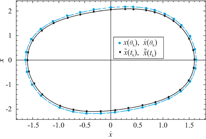

  

  Limit cycle of nonlinear system: the black solid line denotes the limit cycle of the actual response; the blue dotted line denotes the limit cycle predicted by the first-order dynamic frequency

• (II) The analytical relationship expression between $x$ and $\dot{x}$ is determined based on dynamic frequency method

  $$\left\{ \begin{aligned} x = a_{0} \cos \theta + b, \hfill \\ \dot{x} = - a_{0} \omega (\theta )\sin \theta . \hfill \\ \end{aligned} \right.$$

  (27)

• (III) Collect the phase coordinates $(\tilde{x}(t_{k} ),\tilde{\dot{x}}(t_{k} ))$ of the system. Based on the sample data $\tilde{x}(t_{k} )$ and the assumption (I), we can determine the amplitude,

  the bias and the sequence of $\theta_{k}$ in Eq. (27)

  $$a_{0} = \frac{{{\text{max[}}\tilde{x}(t)] - {\text{min[}}\tilde{x}(t)]}}{2},$$

  (28)
  $$b = \frac{{{\text{max[}}\tilde{x}(t)] + {\text{min[}}\tilde{x}(t)]}}{2},$$

  (29)
  $$\theta_{k} = { \arccos }[(\tilde{x}(t_{k} ) - b)/a_{0} ],$$

  (30)

  where $\tilde{x}(t_{k} )$ represents the collected data at the kth point in time domain.

• (IV) Since there is an error between the analytical solution and the actual response, substituting the sequence of $\theta_{k}$ into $\dot{x}$ in Eq. (27), the following deviation will be obtained

  $$R_{k} = \tilde{\dot{x}}(t_{k} ) - \dot{x}(\theta_{k} ) .$$

  (31)

• (V) Calculate the sum of the squares of the above errors, we get

  $$R = \sum\limits_{k = 1}^{N} {R_{k}^{2} } = \sum\limits_{k = 1}^{N} {(\tilde{\dot{x}}(t_{k} ) - \dot{x}(\theta_{k} ))^{2} } ,$$

  (32)

  where $N$ is the total number of the collected data samples. Thus, the unknown parameters in nonlinear oscillator can be identified by the above equation in a least-squares sense.

It can be seen from the above procedure that the accuracy of parameter identification results depends on the accuracy of the optimization algorithm and analytical expression fitting to the response data. Here, the algorithm uses a trust region approach to optimize based on the interior-reflective Newton method. And higher-order analytical approximations can be constructed by using dynamic frequency method.

3.2 Implementation based on numerical data

Here, we use Eq. (26) to investigate the performance of the proposed identification method. The response data is collected by the numerical simulation of Eq. (26), and the group G₂ parameters in Table 1 are taken as the reference values. Given the initial value $x(0) = 0,\;\dot{x}(0) = 1$, we use the Runge–Kutta method to obtain the numerical simulation responses of Eq. (26). A total of $1 \times 10^{4}$ data points are recorded at a 1 kHz sample rate.

For systems with periodic response, the method of multiple scales is a common method to construct the theoretical models [17]. In order to show the performance and advantage of the presented dynamic frequency-based identification approach, we conduct the comparison between the identification result by the presented method and that by the method of multiple scales.

Firstly, we assume that $\alpha_{3} ,$$\beta_{0,1} ,$$\beta_{2,1}$ are unknown values. Then, based on the sampling data at equal time intervals from the numerical simulation results, we obtain the parameter identification results. The comparison between the identified results under the first-order estimation and reference values is shown in Table 2. Table 3 shows the comparison between the identified results under the second-order estimation and reference values. It verifies the efficiency of the presented parameter identification method. Moreover, the accuracy of the second-order estimation is still higher enough even for the strongly nonlinear systems.

Table 2 Identification results of unknown parameters under the first-order estimation

Table 3 Identification results of unknown parameters under the second-order estimation

Next, we discuss the applicability of this method under noisy data. In this case, a uniformly distributed noise with a specified noise-to-signal ratio is added to the simulated response signal. It is assumed that the noise signal is Gaussian white noise, and its amplitude is proportional to the real signal. Denote $x(t)$ as the actual signal, $\hat{x}(t)$ as the noise-containing signal, and $g(t)$ as the unit intensity Gaussian white-noise signal with an average value of zero. It gives

$$\hat{x}(t) = x(t) + e \cdot x(t) \cdot g(t),$$

(33)

where $e$ reflects the intensity of noise.

In Fig. 3, we obtain the numerical simulation response $\hat{x}(t)$ and $\hat{\dot{x}}(t)$ with the noise intensity of $e = 0.05$. The identified results of $\alpha_{3}$ under different noise intensity are shown in Table 4. It shows that the new method is still valid under the noisy environment.

Fig. 3

System response signal of a displacement and b velocity with noise intensity of e = 0.05

Table 4 Identification results of the parameter $\alpha_{3}$ under different noise intensity

4 Experiments

Recently, harvesting vibration energy from the environment via piezoelectric materials has been a promising technology to power macro and micro sensors [18, 20]. Since the ambient vibrations tend to be low-frequency and often have a relatively wide spectrum, the intentional introduction of nonlinearity into energy harvesters has attracted much attentions because of the potential to combine large responses with a wider response in bandwidth as compared to linear oscillators [21, 22].

However, the nonlinear systems exhibit multi-scale behavior in both space and time [23], and the value of some parameters is very important for the design of energy harvester [24]. It must also be assumed that there is uncertainty in the equations of motion, in the specification of parameters, and in the measurements of the system. Accordingly, the viscous damping, linear and nonlinear stiffness coefficients obtained by the theoretical modeling may be not accurate enough to characterize the real sense behaviors of oscillators [25]. Therefore, it is vital to correctly identify those implicit components.

In this section, we focus on determining the control equation of an energy harvester architecture with nonlinearity caused by cantilever-surface contact.

4.1 Experimental device introduction

The apparatus described here is used to investigate the application of this parameter identification method. The experimental device is shown in Fig. 4. Taking into account the elimination of gravity, the cantilever beam is fixed horizontally. The beam’s excitation force is measured by an acceleration transducer attached to the base, and the vibration response is acquired by Laser displacement sensor. The nonlinear oscillator composed of a cantilever beam with a proof mass and two symmetric surfaces with given geometry is shown in Fig. 5a. The piezoelectric transducer in this harvester is composed of a piezoelectric macro-fibre composite (MFC) and a non-piezoelectric (beryllium bronze) layer, which makes it work as a cantilever beam.

Fig. 4

Photograph of the experimental device

Fig. 5

a Schematic drawing of the energy harvester and b schematic cross-sectional view of the cantilever beam

The contact surface shape, modified from the Timoshenko’s design, can be expressed as the following form

$$y_{s} = d_{g} \left(\frac{x}{{L_{s} }}\right)^{5} ,$$

(34)

where $y_{s}$ is the coordinate values of contact surface in the $y$ axial direction, $L_{s}$ is the length of contact surface in the $x$ axial direction, $d_{g}$ is the gap distance between undeflected cantilever and the contact surface at $x = L_{s}$.

The piezoelectric cantilever wraps along the contact surfaces are machined from a 2 mm thick aluminum alloy plate. Figure 5b shows the cross-sectional view, and $L_{c}$ is the length of the cantilever beam. The material and geometrical parameters of the harvester are listed in Table 5.

Table 5 Material parameters and geometry of the energy harvester

4.2 Identification from dynamic frequency solution

The experimental setup imposes a base excitation $y_{b}$ to the harvester, with coordinate $y$ as the displacement. Based on Euler–Bernoulli beam theory and series of discretization methods, the motion equation of the harvester can be written as

$$\begin{aligned} m\ddot{y}(t) + c\dot{y}(t) + F_{R} = - m\ddot{y}_{b} , \hfill \\ y_{b} (t) = Y\sin (\varOmega t), \hfill \\ \end{aligned}$$

(35)

where $y(t)$ represents the motion of the tip mass, $y_{b} (t)$ is the motion of the base, $m$ is the terminal equivalent mass, $c$ is the damping coefficient of the cantilever-surface contact vibration, $Y$ is the base excitation amplitude, $\varOmega$ is the frequency of applied vibration, and $F_{R}$ is the restoring force of the mass, which can be written as a $Z_{2}$ symmetric polynomial form. Nonlinear terms in different models take various forms. According to Ref. [26], the relationship between $F_{R}$ and $y(t)$ of this structure can be obtained by the following equations

$$y(t) = \frac{{F_{R} L_{F}^{3} }}{3EI} + \frac{{\text{d}}S}{{\text{d}}x}\left| {_{{x = x_{d} }} } \right. \cdot L_{F} + y_{s} (x_{d} ),$$

(36)

$$F_{R} = \frac{{20EId_{g} x_{d}^{3} }}{{L_{s}^{5} L_{F} }},$$

(37)

where $x_{d}$ is demarcation point due to the deflection of contact surface and $L_{F} = L_{c} - x_{d}$.

However, by analyzing the response of the system, we realize that it is not purely symmetrical, especially in the case of large-amplitude vibrations, so that the theoretical model based on the symmetry hypothesis is inaccurate to characterize the movement. Therefore, to correctly identify those terms becomes very necessary.

Considering the relative ground coordinate $y(t)$ and its derivatives, $\dot{y}(t)$ and $\ddot{y}(t)$, and the base acceleration $\ddot{y}_{b} (t)$ as the input of the system, the goal of this section is to reconstruct Eq. (35) in the form of a non-Z₂ symmetric model as in Eq. (38) with consideration of the errors in installation and machining. Concerning the establishment of this model, it is crucial to use the prior expert knowledge of the system to select the proper linear and nonlinear basis, and it is common practice to use polynomials

$$\ddot{y} + \beta_{0,1} \dot{y} + \omega_{0}^{2} y + (\alpha_{2} y^{2} + \alpha_{3} y^{3} + \ldots \alpha_{n} y^{n} ) = - \ddot{y}_{b},$$

(38)

where $\omega_{0} ,\;\alpha_{2} ,\;\alpha_{3} ,\; \ldots \;\alpha_{n} ,\beta_{0,1}$ are the unknown parameters.

Considering the characteristics of high accuracy and relatively low computational complexity, we use the second order dynamic frequency method to obtain the expression of limit cycles. That is

$$\left\{ \begin{aligned} y = a_{0} \cos \theta + b, \hfill \\ \dot{y} = - a_{0} (\omega_{1,0} + \omega_{1,1} (\theta ) + \omega_{1,2} (\theta ))\sin \theta . \hfill \\ \end{aligned} \right.$$

(39)

Then we collect the displacement and velocity response sequences at the primary resonance as $(\hat{y}(t_{k} ),\hat{\dot{y}}(t_{k} ))$. It is observed that the primary resonance frequency is 9.7 Hz when the excitation acceleration is 0.1 g. The collected displacement signal $\hat{y}(t_{k} )$ is shown in Fig. 6a. In order to obtain the estimated velocity signal $\hat{\dot{y}}(t_{k} )$ in Fig. 6b, cubic smoothing splines are implemented to avoid noise magnification. It can be seen that the system has a typical steady-state periodic response. After repeated trials and adjustments, the nonlinear order in Eq. (38) is set to $n = 5$.

Fig. 6

Response signal of a displacement and b velocity in the system

After electing the suitable model, we will search for the coefficients to decide the terms that remain in the model. Based on the displacement signal $\hat{y}(t_{k} )$, we obtain $a_{0} = 0.0085$, $b = 0.0011$ and the sequence of $\theta_{k}$ in Eq. (39). Then we use the sequence of $\theta_{k}$ and $\hat{\dot{y}}(t_{k} )$ to identify the unknown parameters $\omega_{0} ,\;\alpha_{2} ,\;\alpha_{3} ,\;\alpha_{4} ,\;\alpha_{5} ,\;\beta_{0,1}$ in a least-squares sense

$$R = \sum\limits_{k = 1}^{N} {(\hat{\dot{y}}(t_{k} } ) - \dot{y}(\theta_{k} ))^{2} .$$

(40)

Table 6 gives the estimate results of those unknown parameters from Eq. (38); Figs. 7 and 8 give the comparison between experimental and numerical simulation results at different frequency. It can be seen that the numerical simulation results are in good agreement with the experimental results. Moreover, in order to verify the validity of the identified parameters, as shown in Fig. 9, the stiffness restoring force of the nonlinear oscillator is measured by a digital dynamometer. Then the restoring force acquired by theoretical and identified model, as well as the experimental values are presented in Fig. 10. It shows that the identified model provides excellent coherence with the measured data as compared with the initial theoretical model.

Table 6 Results of identification based on the second-order estimation

Fig. 7

Comparison of a displacement and b phase diagram between experimental results and numerical simulation at excitation frequency of 9.7 Hz

Fig. 8

Comparison of a displacement and b phase diagram between experimental results and numerical simulation at excitation frequency of 8.6 Hz

Fig. 9

Photograph for measuring the stiffness restoring force of nonlinear oscillator

Fig. 10

Comparison of the stiffness restoring force of nonlinear oscillator

5 Conclusions

In this paper, we propose a dynamic frequency-based parameter identification approach for the nonlinear system. Based on the characteristics of high accuracy and a simple calculation process of dynamic frequency method, the unknown parameters can be identified by fitting the expression to the collected data, which are the value sets of phase coordinate measured in periodic response of the nonlinear oscillator.

The paper then investigates the reliability of the present parameter identification method by using a Duffing-van der Pol oscillator. Parameters are chosen to cause a periodic response that is used for parameter identification. Meanwhile, we study the accuracy of identification under the influence of noise. The results also show that the proposed method presented in this paper can accurately identify the unknown parameters in noisy environments.

Finally, we investigate the application of this approach to a nonlinear beam energy harvester. The unknown parameters in control equation are determined by using the proposed method, and the identification accuracies are demonstrated by comparing restoring force from both simulations and experimental data.

In summary, the present method is shown to be an effective approach for parameter identification of nonlinear oscillator. The limitation for the presented work arises for nonlinear systems with non-periodic responses. A possible future extension of the presented work would be to fit quasiperiodic nonlinear systems. That will be the topic for the further researches.

Appendix A1

$$\varGamma_{0,1} { = } - \left(\frac{{a_{0} \alpha_{2,0} \beta_{0,1} }}{{9\omega_{ 1 , 0}^{2} }} + \frac{{a_{0} b\alpha_{3,0} \beta_{0,1} }}{{3\omega_{ 1 , 0}^{2} }} + \frac{{2a_{0}^{3} \alpha_{4,0} \beta_{0,1} }}{{15\omega_{ 1 , 0}^{2} }} + \frac{{2a_{0} b^{2} \alpha_{4,0} \beta_{0,1} }}{{3\omega_{ 1 , 0}^{2} }} + \frac{{2a_{0}^{3} b\alpha_{5,0} \beta_{0,1} }}{{3\omega_{ 1 , 0}^{2} }} + \frac{{10a_{0} b^{3} \alpha_{5,0} \beta_{0,1} }}{{9\omega_{ 1 , 0}^{2} }}\right),$$

$$\begin{aligned} \varGamma_{ 0 , 2} { = }\frac{{a_{0}^{ 2} \alpha_{ 2,0}^{2} }}{{ 1 8\omega_{ 1 , 0}^{ 3} }} + \frac{{a_{0}^{2} b\alpha_{2,0} \alpha_{3,0} }}{{ 3\omega_{ 1 , 0}^{ 3} }} + \frac{{a_{0}^{2} b^{2} \alpha_{3,0}^{2} }}{{2\omega_{ 1 , 0}^{ 3} }} + \frac{{a_{0}^{4} \alpha_{2,0} \alpha_{4,0} }}{{5\omega_{ 1 , 0}^{ 3} }} + \frac{{2a_{0}^{2} b^{2} \alpha_{2,0} \alpha_{4,0} }}{{3\omega_{ 1 , 0}^{ 3} }} + \frac{{3a_{0}^{4} b\alpha_{3,0} \alpha_{4,0} }}{{5\omega_{ 1 , 0}^{ 3} }} \hfill \\ \begin{array}{*{20}c} {} & {} \\ \end{array} + \frac{{2a_{0}^{2} b^{3} \alpha_{3,0} \alpha_{4,0} }}{{\omega_{ 1 , 0}^{ 3} }} + \frac{{4a_{0}^{6} \alpha_{4,0}^{2} }}{{25\omega_{ 1 , 0}^{ 3} }} + \frac{{6a_{0}^{4} b^{2} \alpha_{4,0}^{2} }}{{5\omega_{ 1 , 0}^{ 3} }} + \frac{{2a_{0}^{ 2} b^{4} \alpha_{4,0}^{2} }}{{\omega_{ 1 , 0}^{ 3} }} + \frac{{a_{0}^{4} b\alpha_{2,0} \alpha_{5,0} }}{{\omega_{ 1 , 0}^{ 3} }} + \frac{{10a_{0}^{2} b^{3} \alpha_{2,0} \alpha_{5,0} }}{{9\omega_{ 1 , 0}^{ 3} }} \hfill \\ \begin{array}{*{20}c} {} & {} \\ \end{array} + \frac{{3a_{0}^{4} b^{2} \alpha_{3,0} \alpha_{5,0} }}{{\omega_{ 1 , 0}^{ 3} }} + \frac{{10a_{0}^{2} b^{4} \alpha_{3,0} \alpha_{5,0} }}{{ 3\omega_{ 1 , 0}^{ 3} }} + \frac{{8a_{0}^{6} b\alpha_{4,0} \alpha_{5,0} }}{{5\omega_{ 1 , 0}^{ 3} }} + \frac{{8a_{0}^{4} b^{3} \alpha_{4,0} \alpha_{5,0} }}{{\omega_{ 1 , 0}^{ 3} }} + \frac{{20a_{0}^{2} b^{5} \alpha_{4,0} \alpha_{5,0} }}{{ 3\omega_{ 1 , 0}^{ 3} }} \hfill \\ \begin{array}{*{20}c} {} & {} \\ \end{array} + \frac{{4a_{0}^{6} b^{2} \alpha_{5,0}^{2} }}{{\omega_{ 1 , 0}^{ 3} }} + \frac{{10a_{0}^{4} b^{4} \alpha_{5,0}^{2} }}{{\omega_{ 1 , 0}^{ 3} }} + \frac{{50a_{0}^{2} b^{6} \alpha_{5,0}^{2} }}{{9\omega_{ 1 , 0}^{ 3} }}, \hfill \\ \end{aligned}$$

$$\varGamma_{0,3} { = }\frac{{a_{0}^{3} \alpha_{4,0} \beta_{0,1} }}{{25\omega_{ 1 , 0}^{2} }} + \frac{{a_{0}^{3} b\alpha_{5,0} \beta_{0,1} }}{{5\omega_{ 1 , 0}^{2} }},$$

$$\begin{aligned} \varGamma_{ 0 , 4} { = } - \left(\frac{{a_{0}^{4} \alpha_{3,0}^{2} }}{{ 3 2\omega_{ 1 , 0}^{ 3} }} + \frac{{a_{0}^{4} \alpha_{2,0} \alpha_{4,0} }}{{15\omega_{ 1 , 0}^{ 3} }} + \frac{{9a_{0}^{4} b\alpha_{4,0} \alpha_{3,0} }}{{20\omega_{ 1 , 0}^{ 3} }} + \frac{{a_{0}^{6} \alpha_{4,0}^{2} }}{{10\omega_{ 1 , 0}^{ 3} }} + \frac{{9a_{0}^{4} b^{2} \alpha_{4,0}^{2} }}{{10\omega_{ 1 , 0}^{ 3} }} + \frac{{a_{0}^{4} b\alpha_{2,0} \alpha_{5,0} }}{{3\omega_{ 1 , 0}^{ 3} }} + \frac{{a_{0}^{6} \alpha_{3,0} \alpha_{5,0} }}{{8\omega_{ 1 , 0}^{ 3} }} \right.\hfill \\ \begin{array}{*{20}c} {} & {} \\ \end{array} \left. + \frac{{13a_{0}^{4} b^{2} \alpha_{3,0} \alpha_{5,0} }}{{8\omega_{ 1 , 0}^{ 3} }} + \frac{{3a_{0}^{6} b\alpha_{4,0} \alpha_{5,0} }}{{2\omega_{ 1 , 0}^{ 3} }} + \frac{{ 3 1a_{0}^{4} b^{3} \alpha_{4,0} \alpha_{5,0} }}{{6\omega_{ 1 , 0}^{ 3} }} + \frac{{a_{0}^{8} \alpha_{5,0}^{5} }}{{8\omega_{ 1 , 0}^{ 3} }} + \frac{{15a_{0}^{6} b^{2} \alpha_{5,0}^{2} }}{{4\omega_{ 1 , 0}^{ 3} }} + \frac{{155a_{0}^{4} b^{4} \alpha_{5,0}^{2} }}{{24\omega_{ 1 , 0}^{ 3} }}\right), \hfill \\ \end{aligned}$$

$$\varGamma_{ 0 , 6} { = }\frac{{a_{0}^{6} \alpha_{4,0}^{2} }}{{ 5 0\omega_{ 1 , 0}^{ 3} }} + \frac{{a_{0}^{6} \alpha_{3,0} \alpha_{5,0} }}{{24\omega_{ 1 , 0}^{ 3} }} + \frac{{11a_{0}^{6} b\alpha_{4,0} \alpha_{5,0} }}{{30\omega_{ 1 , 0}^{ 3} }} + \frac{{a_{0}^{8} \alpha_{5,0}^{2} }}{{12\omega_{ 1 , 0}^{ 3} }} + \frac{{11a_{0}^{6} b^{2} \alpha_{5,0}^{2} }}{{12\omega_{ 1 , 0}^{ 3} }},$$

$$\varGamma_{0,8} { = } - \frac{{a_{0}^{8} \alpha_{5,0}^{2} }}{{72\omega_{1,0}^{3} }},$$

$$\varGamma_{ 1 , 1} { = } - \left(\frac{{a_{0}^{2} \alpha_{3,0} \beta_{0,1} }}{{16\omega_{ 1 , 0}^{2} }} + \frac{{a_{0}^{2} b\alpha_{4,0} \beta_{0,1} }}{{4\omega_{ 1 , 0}^{2} }} + \frac{{13a_{0}^{4} \alpha_{5,0} \beta_{0,1} }}{{144\omega_{ 1 , 0}^{2} }} + \frac{{5a_{0}^{2} b^{2} \alpha_{5,0} \beta_{0,1} }}{{8\omega_{ 1 , 0}^{2} }}\right),$$

$$\begin{aligned} \varGamma_{ 1 , 2} { = }\frac{{a_{0}^{3} \alpha_{2,0} \alpha_{3,0} }}{{12\omega_{ 1 , 0}^{ 3} }} + \frac{{a_{0}^{3} b\alpha_{3,0}^{2} }}{{4\omega_{ 1 , 0}^{ 3} }} + \frac{{a_{0}^{3} b\alpha_{2,0} \alpha_{4,0} }}{{3\omega_{ 1 , 0}^{ 3} }} + \frac{{a_{0}^{5} \alpha_{3,0} \alpha_{4,0} }}{{10\omega_{ 1 , 0}^{ 3} }} + \frac{{3a_{0}^{3} b^{2} \alpha_{3,0} \alpha_{4,0} }}{{2\omega_{ 1 , 0}^{ 3} }} \hfill \\ \begin{array}{*{20}c} {} & {} \\ \end{array} + \frac{{2a_{0}^{5} b\alpha_{4,0}^{2} }}{{5\omega_{ 1 , 0}^{ 3} }} + \frac{{2a_{0}^{3} b^{3} \alpha_{4,0}^{2} }}{{\omega_{ 1 , 0}^{ 3} }} + \frac{{a_{0}^{5} \alpha_{2,0} \alpha_{5,0} }}{{6\omega_{ 1 , 0}^{ 3} }} + \frac{{5a_{0}^{3} b^{2} \alpha_{2,0} \alpha_{5,0} }}{{6\omega_{ 1 , 0}^{ 3} }} + \frac{{a_{0}^{5} b\alpha_{3,0} \alpha_{5,0} }}{{\omega_{ 1 , 0}^{ 3} }} \hfill \\ \begin{array}{*{20}c} {} & {} \\ \end{array} + \frac{{10a_{0}^{3} b^{3} \alpha_{3,0} \alpha_{5,0} }}{{3\omega_{ 1 , 0}^{ 3} }} + \frac{{a_{0}^{7} \alpha_{4,0} \alpha_{5,0} }}{{5\omega_{ 1 , 0}^{ 3} }} + \frac{{4a_{0}^{5} b^{2} \alpha_{4,0} \alpha_{5,0} }}{{\omega_{ 1 , 0}^{ 3} }} + \frac{{25a_{0}^{3} b^{4} \alpha_{4,0} \alpha_{5,0} }}{{3\omega_{ 1 , 0}^{ 3} }} \hfill \\ \begin{array}{*{20}c} {} & {} \\ \end{array} + \frac{{a_{0}^{7} b\alpha_{5,0}^{2} }}{{\omega_{ 1 , 0}^{ 3} }} + \frac{{20a_{0}^{5} b^{3} \alpha_{5,0}^{2} }}{{3\omega_{ 1 , 0}^{ 3} }} + \frac{{25a_{0}^{3} b^{5} \alpha_{5,0}^{2} }}{{3\omega_{ 1 , 0}^{ 3} }}, \hfill \\ \end{aligned}$$

$$\varGamma_{ 1 , 3} { = }\frac{{a_{0}^{4} \alpha_{5,0} \beta_{0,1} }}{{36\omega_{ 1 , 0}^{2} }},$$

$$\begin{aligned} \varGamma_{ 1 , 4} { = } - (\frac{{a_{0}^{5} \alpha_{3,0} \alpha_{4,0} }}{{ 2 0\omega_{ 1 , 0}^{ 3} }} + \frac{{a_{0}^{5} b\alpha_{4,0}^{2} }}{{5\omega_{ 1 , 0}^{ 3} }} + \frac{{a_{0}^{5} \alpha_{2,0} \alpha_{5,0} }}{{18\omega_{ 1 , 0}^{ 3} }} + \frac{{5a_{0}^{5} b\alpha_{3,0} \alpha_{5,0} }}{{12\omega_{ 1 , 0}^{ 3} }} + \frac{{a_{0}^{7} \alpha_{4,0} \alpha_{5,0} }}{{6\omega_{ 1 , 0}^{ 3} }} \hfill \\ \begin{array}{*{20}c} {} & {} \\ \end{array} + \frac{{11a_{0}^{5} b^{2} \alpha_{4,0} \alpha_{5,0} }}{{6\omega_{ 1 , 0}^{ 3} }} + \frac{{5a_{0}^{7} b\alpha_{5,0}^{2} }}{{6\omega_{ 1 , 0}^{ 3} }} + \frac{{55a_{0}^{5} b^{3} \alpha_{5,0}^{2} }}{{18\omega_{ 1 , 0}^{ 3} }}), \hfill \\ \end{aligned}$$

$$\varGamma_{ 1 , 6} { = }\frac{{a_{0}^{ 7} \alpha_{ 4,0} \alpha_{ 5,0} }}{{ 3 0\omega_{ 1 , 0}^{ 3} }} + \frac{{a_{0}^{ 7} b\alpha_{ 5,0}^{2} }}{{ 6\omega_{ 1 , 0}^{ 3} }}.$$

References

Gaëtan, K., Worden, K., Vakakis, A.F.: Past, present and future of nonlinear system identification in structural dynamics. Mech Syst Signal Pr. 20, 505–592 (2016)
Ge, X.B., Luo, Z., Ma, Y.: A novel data-driven model based parameter estimation of nonlinear systems. J. Sound Vib. 453, 188–200 (2019)
Thothadri, M., Casas, R.A., Moon, F.C.: Nonlinear system identification of multi-degree-of-freedom systems. Nonlinear Dyn. 32, 307–322 (2003)
Xu, L.: The damping iterative parameter identification method for dynamical systems based on the sine signal measurement. Signal Process. 120, 660–667 (2016)
Moore, K.J., Kurt, M., Eriten, M., et al.: Nonlinear parameter identification of a mechanical interface based on primary wave scattering. Exp. Mech. 57, 1495–1508 (2017)
Do, T.N., Tjahjowidodo, T., Lau, M.W.S.: A new approach of friction model for tendon-sheath actuated surgical systems: nonlinear modelling and parameter identification. Mech. Mach. Theor. 85, 13–24 (2015)
Thothadri, M., Moon, F.C.: Nonlinear system identification of systems with periodic limit-cycle response. Nonlinear Dyn. 39, 63–77 (2005)
Leontaritis, I.J., Billings, S.A.: Input-output parametric models for nonlinear systems. Int. J. Control 41, 303–328 (1985)
Masri, S.F., Caughey, T.K.: A nonparametric identification technique for nonlinear dynamic problems. J. Appl. Mech. 46, 433–447 (1979)
Mann, B.P., Khasawneh, F.A.: An energy-balance approach for oscillator parameter identification. J. Sound Vib. 321, 65–78 (2009)
Peng, J., Peng, Z.: Parameter identification of strongly nonlinear vibration systems of 2-dof. J Dyn Control. 5, 54–56 (2007)
Dou, S.G., Ye, M., Zhang, W.: Nonlinearity system identification method with parametric excitation based on the incremental harmonic balance method. J Theor App Mech-Pol. 42, 332–336 (2010)
Tang, L., Yang, Y., Wu, H.: Modeling and experiment of a multiple-dof piezoelectric energy harvester. J. Opt. Soc. Am. A 8341, 39 (2012)
Perona, P., Porporato, A., Ridolfi, L.: On the trajectory method for the reconstruction of differential equations from time series. Nolinear Dyn. 23, 13–33 (2000)
Zhang, Z.W., Wang, Y.J., Wang, W.: Periodic solution of the strongly nonlinear asymmetry system with the dynamic frequency method. Symmetry. 11, 676 (2019)
Chen, S.H., Chen, Y.Y., Szw, K.Y.: A hyperbolic perturbation method for determining homoclinic solution of certain strongly nonlinear autonomous oscillators. J. Sound Vib. 322, 381–392 (2009)
Meesala, V.C., Hajj, M.R.: Identification of nonlinear piezoelectric coefficients. J. Appl. Phys. 124, 065112 (2018)
Yao, M.H., Liu, P.F., Zhang, W.: Power generation capacity analysis of three kinds of piezoelectric vibration cantilever beams: comparison study. Adv. Mater. Sci. Eng. 26(28), 4880–4887 (2017)
Zou, H.X., Zhang, W.M.: Magnetically coupled flextensional transducer for wideband vibration energy harvesting: design, modeling and experiments. J. Sound Vib. 416, 55–79 (2018)
Cao, D.X., Gao, Y.H., Hu, W.H.: Modeling and power performance improvement of a piezoelectric energy harvester for low-frequency vibration environments. Acta. Mech. Sin. 35, 894–911 (2019)
Yao, M.H., Ma, L., Zhang, W.: Study on power generations and dynamic responses of the bistable straight beam and the bistable L-shaped beam. Sci. China Technol. Sci. 61, 1404–1416 (2018)
Wang, C., Zhang, Q.C., Wang, W.: Low-frequency wideband vibration energy harvesting by using frequency up-conversion and quin-stable nonlinearity. J. Sound Vib. 399, 169–181 (2017)
Wang, Y.J., Zhang, Q.C., Wang, W., Yang, T.Z.: In-plane dynamics of a fluid-conveying corrugated pipe supported at both ends. Appl. Math. Mech-Engl. 40, 1119–1134 (2019)
Yuan, T.C., Yang, J., Chen, L.Q.: Nonparametric identification of nonlinear piezoelectric mechanical systems. J. Appl. Mech. 85, 111008 (2018)
Brunton, S.L., Nathan, K.J.: Data-driven science and engineering: machine learning, dynamical systems, and control. Cambridge University Press, Cambridge (2019)
Wang, C., Zhang, Q.C., Wang, W.: A low-frequency, wideband quad-stable energy harvester using combined nonlinearity and frequency up-conversion by cantilever-surface contact. Mech. Syst. Signal Process. 112, 305–318 (2018)
Acknowledgement
This work was supported by the National Natural Science Foundation of China (Grants 11772218 and 11872044), China-UK NSFC-RS Joint Project (Grants 11911530177 in China and IE181496 in UK), Tianjin Research Program of Application Foundation and Advanced Technology (Grant 17JCYBJC18900), and the National Key Research and Development Program of China (Grant 2018YFB0106200).
Author information
Authors and Affiliations
Corresponding author
Appendix A1
Rights and permissions
About this article
Cite this article
Zhang, Z., Wang, W. & Wang, C. Parameter identification of nonlinear system via a dynamic frequency approach and its energy harvester application. Acta Mech. Sin. 36, 606–617 (2020). https://doi.org/10.1007/s10409-020-00972-1
Received:
Revised:
Accepted:
Published:
Issue Date:
DOI: https://doi.org/10.1007/s10409-020-00972-1