
Abstract
We prove that the geodesic equations of all Sobolev metrics of fractional order one and higher on spaces of diffeomorphisms and, more generally, immersions are locally well posed. This result builds on the recently established real analytic dependence of fractional Laplacians on the underlying Riemannian metric. It extends several previous results and applies to a wide range of variational partial differential equations, including the well-known Euler–Arnold equations on diffeomorphism groups as well as the geodesic equations on spaces of manifold-valued curves and surfaces.
1 Introduction
1.1 Background
Many prominent partial differential equations (PDEs) in hydrodynamics admit variational formulations as geodesic equations on an infinite-dimensional manifold of mappings. These include the incompressible Euler [2], Burgers [35], modified Constantin–Lax–Majda [14, 19, 61], Camassa–Holm [17, 39, 48], Hunter–Saxton [30, 43], surface quasi-geostrophic [20, 60] and Korteweg–de Vries [51] equations of fluid dynamics as well as the governing equation of ideal magneto-hydrodynamics [44, 59]. This serves as a strong motivation for the study of Riemannian geometry on mapping space. An additional motivation stems from the field of mathematical shape analysis, which is intimately connected to diffeomorphisms groups and other infinite-dimensional mapping spaces via Grenander’s pattern theory [27, 63] and elasticity theory [9, 53].
The variational formulations allow one to study analytical properties of the PDEs in relation to geometric properties of the underlying infinite-dimensional Riemannian manifold [4, 5, 13, 34, 49, 52]. Most importantly, local well-posedness of the PDE, including smooth dependence on initial conditions, is closely related to smoothness of the geodesic spray on Sobolev completions of the configuration space [23]. This has been used to show local well-posedness of PDEs in many specific examples, cf. the recent overview article [38]. An extension of this successful methodology to wider classes of PDEs requires an in-depth study of smoothness properties of partial and pseudo differential operators with non-smooth coefficients such as those appearing in the geodesic spray or, more generally, in the Euler–Lagrange equations. This is the topic of the present paper.
1.2 Contribution
This article establishes local well-posedness of the geodesic equation for fractional order Sobolev metrics on spaces of diffeomorphisms and, more generally, immersions. A simplified version of our main result reads as follows:
Theorem
On the space of immersions of a closed manifold M into a Riemannian manifold \((N,\bar{g})\), the geodesic equation of the fractional-order Sobolev metric
is locally well-posed in the sense of Hadamard for any \(p\in [1,\infty )\).
This follows from Theorems 4.4 and 4.6. The result unifies and extends several previously known results:
For integer-order metrics, local well-posedness on the space of immersions from M to N has been shown in [11]. However, the proof contained a gap, which was closed in [50] for \(N={\mathbb {R}}^n\), and which is closed in the present article for general N. The strategy of proof, which goes back to Ebin and Marsden [23], is to show that the geodesic spray extends smoothly to certain Sobolev completions of the space. Our generalization to fractional-order metrics builds on recent results about the smoothness of the functional calculus of sectorial operators [6].
For \(N={\mathbb {R}}^n\), the set of N-valued immersions becomes a vector space, which simplifies the formulation of the geodesic equation; see Corollary 5.3. The treatment of general manifolds N requires a theory of Sobolev mappings between manifolds, which is developed in Sect. 2.2. Moreover, in the absence of global coordinate systems for these mapping spaces, we recast the geodesic equation using an auxiliary covariant derivative following [11]; see Lemma 2.6 and Theorem 4.3.
For \(M=N\) our result specializes to the diffeomorphism group \({\text {Diff}}(M)\), which is an open subset of \({\text {Imm}}(M,M)\). On \({\text {Diff}}(M)\) we obtain local well-posedness of the geodesic equation for Sobolev metrics of order \(p\in [1/2,\infty )\); see Corollary 5.1. Analogous results have been obtained by different methods (smoothness of right-trivializations) for inertia operators that are defined as abstract pseudo-differential operators [3, 10, 24].
For \(M=S^1\), our result specializes to the space of immersed loops in N. For loops in \(N={\mathbb {R}}^d\), local well-posedness has been shown by different methods (reparameterization to arc length) in [8]. Our analysis extends this result to manifold-valued loops and also to higher-dimensional and more general base manifolds M.
2 Sobolev mappings
2.1 Setting
We use the notation of [11] and write \({\mathbb {N}}\) for the natural numbers including zero. Smooth will mean \(C^\infty \) and real analytic \(C^\omega \). Sobolev regularity is denoted by \(H^r\), and Sobolev spaces \(H^s_{H^r}\) of mixed order r in the foot point and s in the fiber are introduced in Theorem 2.4.
Throughout this paper, without any further mention, we fix a real analytic connected closed manifold M of dimension \({\text {dim}}(M)\) and a real analytic manifold N of dimension \({\text {dim}}(N)\ge {\text {dim}}(M)\).
2.2 Sobolev sections of vector bundles
[6, Section 2.3] We write \(H^s(\mathbb R^m,{\mathbb {R}}^n)\) for the Sobolev space of order \(s\in {\mathbb {R}}\) of \({\mathbb {R}}^n\)-valued functions on \({\mathbb {R}}^m\). We will now generalize these spaces to sections of vector bundles. Let E be a vector bundle of rank \(n\in {\mathbb {N}}_{>0}\) over M. We choose a finite vector bundle atlas and a subordinate partition of unity in the following way. Let \((u_i:U_i \rightarrow u_i(U_i)\subseteq \mathbb R^m)_{i\in I}\) be a finite atlas for M, let \((\varphi _i)_{i\in I}\) be a smooth partition of unity subordinated to \((U_i)_{i \in I}\), and let \(\psi _i:E|U_i \rightarrow U_i\times {\mathbb {R}}^n\) be vector bundle charts. Note that we can choose open sets \(U_i^\circ \) such that \({\text {supp}}(\psi _i)\subset U_i^\circ \subset \overline{U_i^\circ }\subset U_i\) and each \(u_i(U_i^\circ )\) is an open set in \({\mathbb {R}}^m\) with Lipschitz boundary (cf. [15, Appendix H3]). Then we define for each \(s \in {\mathbb {R}}\) and \(f \in \Gamma (E)\)
Then \(\Vert \cdot \Vert _{\Gamma _{H^s}(E)}\) is a norm, which comes from a scalar product, and we write \(\Gamma _{H^s}(E)\) for the Hilbert completion of \(\Gamma (E)\) under the norm. It turns out that \(\Gamma _{H^s}(E)\) is independent of the choice of atlas and partition of unity, up to equivalence of norms. We refer to [58, Section 7] and [28, Section 6.2] for further details.
The following theorem describes module properties of Sobolev sections of vector bundles, which will be used repeatedly throughout the paper.
2.3 Theorem
Module properties. [6, Theorem 2.4] Let \(E_1,E_2\) be vector bundles over M and let \(s_1,s_2,s\in {\mathbb {R}}\) satisfy
Then the tensor product of smooth sections extends to a bounded bilinear mapping
The following theorem describes the manifold structure of Sobolev mappings between finite-dimensional manifolds. It is an elaboration of [46, 5.2 and 5.4] and an extension to the Sobolev case of parts of [41, Section 42].
2.4 Theorem
Sobolev mappings between manifolds. The following statements hold for any \(r\in ({\text {dim}}(M)/2,\infty )\) and \(s,s_1,s_2 \in [-r,r]\):
- (a):
The space \(H^{r}(M,N)\) is a \(C^{\infty }\) and a real analytic manifold. Its tangent space satisfies in a natural (i.e., functorial) way
with foot point projection given by \(\pi _{H^{r}}(M,N)=(\pi _N)_*:h \mapsto \pi _N\circ h\).
- (b):
The space \(H^s_{H^r}(M,TN)\) of ‘\(H^s\) mappings \(M\rightarrow TN\) with foot point in \(H^{r}(M,N)\)’ is a real analytic manifold and a real analytic vector bundle over \(H^{r}(M,N)\). Similarly, spaces such as \(L(H^{s_1}_{H^r}(M,TN),H^{s_2}_{H^r}(M,TN))\) are real analytic vector bundles over \(H^{r}(M,N)\).
- (c):
The space \({\text {Met}}_{H^{r}}(M)\) of all Riemannian metrics of Sobolev regularity \(H^r\) is an open subset of the Hilbert space \(\Gamma _{H^r}(S^2T^*M)\), and thus a real analytic manifold.

Proof
- (a):
-
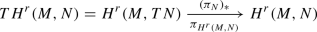
Let us recall the chart construction: we use an auxiliary real analytic Riemannian metric \( {\hat{g}}\) on N and its exponential mapping \(\exp ^{ {\hat{g}}}\); some of its properties are summarized in the following diagram:

Without loss we may assume that \(V^{N\times N}\) is symmetric:
$$\begin{aligned} (y_1,y_2)\in V^{N\times N} \iff (y_2,y_1)\in V^{N\times N}. \end{aligned}$$A chart, centered at a real analytic \(f\in C^\omega (M,N)\), is:

Note that \({\tilde{U}}_f\) is open in \(\Gamma (f^*TN)\). The charts \(U_f\) for \(f\in C^\omega (M,N)\) cover \(H^r(M,N)\): since \(C^\omega (M,N)\) is dense in \(H^r(M,N)\) by [41, 42.7] and since \(H^r(M,N)\) is continuously embedded in \(C^{0}(M,N)\), a suitable \(C^0\)-norm neighborhood of \(g\in H^r(M,N)\) contains a real analytic \(f \in C^\omega (M,N)\), thus \(f\in U_g\), and by symmetry of \(V^{N\times N}\) we have \(g\in U_f\). The chart changes,
$$\begin{aligned} \Gamma _{H^r}( f_1^*TN)\supset {\tilde{U}}_{f_1}\ni s \mapsto (u_{f_2,f_1})_*(s) {:=} (\exp ^{ {\hat{g}}}_{f_2})^{-1}\circ \exp ^{ {\hat{g}}}_{f_1}\circ s\in {\tilde{U}}_{f_2}\subset \Gamma _{H^r}( f_2^*TN), \end{aligned}$$for charts centered on real analytic \(f_1,f_2\in C^\omega (M,N)\) are real analytic by Lemma A.5 since \(r>{\text {dim}}(M)/2\). The tangent bundle \(TH^r(M,N)\) is canonically glued from the following vector bundle chart changes, which are real analytic by Lemma A.5 again:
$$\begin{aligned}&{\tilde{U}}_{f_1}\times \Gamma _{H^r}( f_1^*TN) \ni (s, h) \mapsto (T (u_{f_2,f_1})_*)(s,h)= \nonumber \\&\quad =\big ((u_{f_2,f_1})_*(s), (d_{\text {fiber}} u_{f_2,f_1})_*(s,h)\big )\in {\tilde{U}}_{f_2}\times \Gamma _{H^r}( f_2^*TN) \end{aligned}$$(1)It has the canonical charts

These identify \(TH^r(M,N)\) canonically with \(H^r(M,TN)\) since
$$\begin{aligned} Tu_f^{-1}(s,s') = T(\exp _f^{ {\hat{g}}})\circ {\text {vl}}\circ (s,s'):M\rightarrow TN\,, \end{aligned}$$where we used the vertical lift \({\text {vl}}:TN\times _N TN \rightarrow TTN\) which is given by \({\text {vl}}(u_x,v_x)= \partial _t|_{t=0}(u_x+t.v_x)\); see [45, 8.12 or 8.13]. The corresponding foot-point projection is then
$$\begin{aligned} \pi _{H^s(M,N)}(T(\exp _f^{ {\hat{g}}})\circ {\text {vl}}\circ (s,s'))= \exp _f^{ {\hat{g}}}\circ s = \pi _N\circ T(\exp _f^{ {\hat{g}}})\circ (s,s'). \end{aligned}$$ - (b):
-
The canonical chart changes (1) for \(TH^r(M,N)\) extend to
$$\begin{aligned}&{\tilde{U}}_{f_1}\times \Gamma _{H^s}( f_1^*TN) \ni (s, h) \mapsto (T u_{f_2,f_1})_*(s,h) = \\&\quad =\big ((u_{f_2,f_1})_*(s), (d_{\text {fiber}} u_{f_2,f_1}\circ s)_*(h)\big )\in {\tilde{U}}_{f_2}\times \Gamma _{H^s}( f_2^*TN), \end{aligned}$$since \(d_{\text {fiber}}u_{f_2,f_1}:f_1^*TN\times _M f_1^*TN = f_1^* (TN\times _N TN)\rightarrow f_2^* TN\) is fiber respecting real analytic by the module properties 2.3. Note that \(d_{\text {fiber}}u_{f_2,f_1}\circ s\) is then an \(H^r\)-section of the bundle \(L(f_1^*TN,f_1^*TN)\rightarrow M\), which may be applied to the \(H^s\)-section h by the module properties 2.3. These extended chart changes then glue the vector bundle
$$\begin{aligned} H^s_{H^r}(M,TN)\xrightarrow {(\pi _N)_*} H^r(M,TN). \end{aligned}$$ - (c):
-
The space \(\Gamma _{H^r}(S^2T^*M)\) is continuously embedded in \(\Gamma _{C^1}(S^2T^*M)\) because \(r>{\text {dim}}(M)/2+1\). Thus, the space of metrics is open.


\(\square \)
2.3 Connections, connectors, and sprays
This sections reviews some relations between connections, connectors, and sprays. It holds for general convenient manifolds N, including infinite-dimensional manifolds of mappings, and will be used in this generality in the sequel (see e.g. the proofs of Theorems 4.3 and 4.4).
- (a):
Connectors. [45, 22.8–9] Any connection \(\nabla \) on TN is given in terms of a connector \(K:TTN\rightarrow TN\) as follows: For any manifold M and function \(h:M\rightarrow TN\), one has \(\nabla h = K \circ Th:TM\rightarrow TN\). In the subsequent points we fix such a connection and connector on N.
- (b):
Pull-backs. [45, (22.9.6)] For any manifold Q, smooth mapping \(g:Q\rightarrow M\) and \(Z_y\in T_yQ\), one has \(\nabla _{Tg.Z_y}s = \nabla _{Z_y}(s\circ g)\). Thus, for g-related vector fields \(Z\in {\mathfrak {X}}(Q)\) and \(X\in {\mathfrak {X}}(M)\), one has \(\nabla _Z(s\circ g) = (\nabla _Xs)\circ g\), as summarized in the following diagram:
- (c):
Torsion. [45, (22.10.4)] For any smooth mapping \(f:M\rightarrow N\) and vector fields \(X,Y\in {\mathfrak {X}}(M)\) we have
$$\begin{aligned} {\text {Tor}}(Tf.X,Tf.Y)&=\nabla _X(Tf\circ Y) - \nabla _Y(Tf\circ X) - Tf\circ [X,Y] \\ {}&= (K \circ \kappa _M - K) \circ TTf\circ TX \circ Y. \end{aligned}$$- (d):
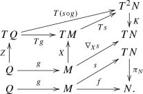
Sprays. [45, 22.7] Any connection \(\nabla \) induces a one-to-one correspondence between fiber-wise quadratic \(C^\alpha \) mappings \(\Phi :TN\rightarrow TN\) and \(C^\alpha \) sprays \(S:TN\rightarrow TTN\). Here \(\nabla _{\partial _t}c_t = \Phi (c_t)\) corresponds to \(c_{tt}=S(c_t)\) for curves c in N. Equivalently, in terms of the connector K, the relation between \(\Phi \) and S is as follows:
The diagram on the left introduces the projections \(T(\pi _N)\) and \(\pi _{TN}\), which define the two vector bundle structures on TTN. The diagram on the right shows that \(\Phi \) and S are related by \(\Phi =K\circ S\).


The following lemma describes how any connection on TN induces via a product-preserving functor from finite to infinite-dimensional manifolds [37, 40] a connection on the mapping space \(H^s_{H^r}(M,TN)\). The induced connection will be used as an auxiliary tool for expressing the geodesic equation; see Theorem 4.3.
2.6 Lemma
Induced connection on mapping spaces. Let \(r \in ({\text {dim}}(M)/2,\infty )\), \(s \in [-r,r]\), and \(\alpha \in \{\infty ,\omega \}\). Then any \(C^\alpha \) connection on TN induces in a natural (i.e., functorial) way a \(C^\alpha \) connection on \(H^s_{H^r}(M,TN)\).
Proof
Note that \(TN\mapsto H^s_{H^r}(M,TN)\) is a product-preserving functor from finite-dimensional manifolds to infinite-dimensional manifolds as described in [40] and [41, Section 31]. Furthermore, note that \(TH^s_{H^r}(M,TN)=H^{r,s,r,s}(M,TTN)\), where (r, s, r, s) denotes the Sobolev regularity of the individual components in any local trivialization \(TTN\supset TTU \xrightarrow {TTu} u(U)\times ({\mathbb {R}}^n)^3\subset ({\mathbb {R}}^n)^4\) induced by a chart \(N\supset U\xrightarrow {u}u(U)\subset \mathbb R^n\); cf. the proof of Theorem 2.4. Applying the functor \(H^s_{H^r}(M,\cdot )\) to the connector \(K:TTN\rightarrow TN\) gives the induced connector
The induced connector is \(C^\alpha \) by Lemma A.5. \(\square \)
3 Sobolev immersions
This section collects some results about the differential geometry of immersions with Sobolev regularity. More specifically, it describes the Sobolev regularity of the induced metric, volume form, normal and tangential projections, and fractional Laplacian, as well as variations of these objects with respect to the immersion. Here the term fractional Laplacian is understood as a p-th power of the operator \(1+\Delta \), where \(\Delta \) is the Bochner Laplacian and \(p \in {\mathbb {R}}\); see [6, Section 3].
3.1 Lemma
Geometry of Sobolev immersions. The following statements hold for any \(r \in ({\text {dim}}(M)/2+1,\infty )\) and any smooth Riemannian metric \(\bar{g}\) on N:
- (a):
The space \({\text {Imm}}_{H^{r}}(M,N)\) of all immersions \(f:M\rightarrow N\) of Sobolev class \(H^{r}\) is an open subset of the real analytic manifold \(H^{r}(M,N)\).
- (b):
The pull-back metric is well defined and real analytic as a mapping
$$\begin{aligned} {\text {Imm}}^r(M,N) \ni f \mapsto f^*\bar{g}\in {\text {Met}}_{H^{r-1}}(M) := \Gamma _{H^{r-1}}(S^2_+T^*M). \end{aligned}$$- (c):
The Riemannian volume form is well defined and real analytic as a mapping
$$\begin{aligned} {\text {Imm}}^r(M,N) \ni f \mapsto {\text {vol}}^{f^*\bar{g}} \in \Gamma _{H^{r-1}}({\text {Vol}}M). \end{aligned}$$- (d):
The tangential projection \(\top :T{\text {Imm}}(M,N)\rightarrow {\mathfrak {X}}(M)\) and the normal projection \(\bot :T{\text {Imm}}(M,N)\rightarrow T{\text {Imm}}(M,N)\) are defined for smooth \(h\in T_f{\text {Imm}}(M,N)\) via the relation \(h = Tf.h^\top +h^\bot \), where \(\bar{g}(h^\bot (x),T_xf(T_xM))=0\) for all \(x\in M\). They extend real analytically for any real number \(s\in [1-r,r-1]\) to
$$\begin{aligned}&\bot \in \Gamma _{C^{\omega }}\Big (L(H^s_{{\text {Imm}}^r}(M,TN),H^s_{{\text {Imm}}^r}(M,TN))\Big ),\\&\top \in C^{\omega }\Big (H^s_{{\text {Imm}}^r}(M,TN), {\mathfrak {X}}_{H^s}(M)\Big ), \end{aligned}$$where \(H^s_{{\text {Imm}}^r}(M,TN)\) is the space of ‘\(H^s\) mappings \(M\rightarrow TN\) with foot point in \({\text {Imm}}^r(M,N)\)’ described in Theorem 2.4.
- (e):
For any real numbers s, p with \(s, s-2p \in [1-r,r]\), the fractional Laplacian
$$\begin{aligned} f\mapsto (1+\Delta ^{f^*\bar{g}})^p \end{aligned}$$is a real analytic section of the bundle
$$\begin{aligned} GL(H^s_{{\text {Imm}}^r}(M,TN),H^{s-2p}_{{\text {Imm}}^r}(M,TN)). \end{aligned}$$
Proof
- (a):
-
The space \(H^r(M,N)\) is continuously embedded in \(C^1(M,N)\) because \(r>{\text {dim}}(M)/2+1\). Thus, the space of immersions is open.
- (b):
-
follows from the formula \(f^*\bar{g}=\bar{g}(Tf,Tf)\).
- (c):
-
follows from (b) and the real analyticity of \(g \mapsto {\text {vol}}^g\); see [6, Lemma 3.3].
- (d):
-
Let U be an open subset of M which carries a local frame \(X \in \Gamma (GL({\mathbb {R}}^m,TU))\). For any \(f \in {\text {Imm}}^{r}(M,N)\), the Gram-Schmidt algorithm transforms X into an \((f^*\bar{g})\)-orthonormal frame \(Y_f\in \Gamma _{H^{r-1}}(GL({\mathbb {R}}^m,TU))\), which is given by
$$\begin{aligned} \forall j \in \{1,\dots ,m\}: \qquad Y_f^j=\frac{X^j-\sum _{k=1}^{j-1} (f^*\bar{g})(Y_f^k,X^j) Y_f^k}{\left\| X^j-\sum _{k=1}^{j-1} (f^*\bar{g})(Y_f^k,X^j) Y_f^j\right\| _{f^*\bar{g}}}. \end{aligned}$$This defines a real analytic map
$$\begin{aligned} Y:{\text {Imm}}^r(M,N) \rightarrow \Gamma _{H^{r-1}}(GL({\mathbb {R}}^m,TU)). \end{aligned}$$We write TN as a sub-bundle of a trivial bundle \(N\times V\) and denote the corresponding inclusion and projection mappings by
$$\begin{aligned} i:TN \rightarrow N \times V, \qquad \pi :N\times V \rightarrow TN. \end{aligned}$$This allows one to define a projection from \(N\times V\) onto TN and further onto the normal bundle of f, which is real analytic as a map
$$\begin{aligned} p:{\text {Imm}}^r(M,N)&\rightarrow H^{r-1}(U,L(V,V)),\\ p_f(x)(v)&:= v-\sum _{i=1}^m \bar{g}\big (\pi (f(x),v), T_xf.Y_f^i(x)\big ). \end{aligned}$$This construction can be repeated for any open set \({\tilde{U}}\) such that \(T{\tilde{U}}\) is parallelizable, and the resulting projections \(p_f\) coincide on \(U\cap {\tilde{U}}\). Thus, one obtains a real analytic map
$$\begin{aligned} p:{\text {Imm}}^r(M,N) \rightarrow H^{r-1}(M,L(V,V)). \end{aligned}$$By the module properties 2.3, this induces a real analytic map
$$\begin{aligned} {\tilde{p}}:{\text {Imm}}^r(M,N) \times H^s(M,V) \rightarrow H^s(M,V), \quad {\tilde{p}}(f,h) := p_f.h. \end{aligned}$$These maps fit into the commutative diagrams
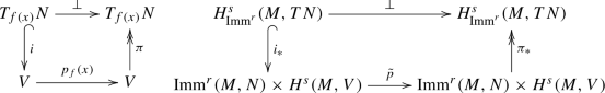
The maps \(i_*\) and \(\pi _*\) are real analytic, as shown in part (b’) of the proof of Lemma A.5. Therefore, the map \(\bot =\pi _*\circ {\tilde{p}} \circ i_*\) is real analytic. The tangential projection \(h^\top = Tf^{-1}(h-h^\bot )\) is then also real analytic.
- (e):
-
There is a bundle E over N such that \(TN\oplus E\) is a trivial bundle, i.e., \(TN\oplus E \cong N\times V\) for some vector space V. We endow the bundle E with a smooth connection and the bundle \(N\times V \cong TN\oplus E\) with the product connection. By construction, the inclusion \(i:TN\rightarrow N\times V\) and projection \(\pi :N\times V \rightarrow TN\) respect the connection. At the level of Sobolev sections of these bundles, this means that the natural inclusion and projection mappings fit into the following commutative diagram with \(p=1\):

As the functional calculus preserves commutation relations, this extends to all p. Thus, we have reduced the situation to the bottom row of the diagram, where the fractional Laplacian acts on \(H^s(M,V)\). In this case real analytic dependence of the fractional Laplacian on the metric has been shown in [6, Theorem 5.4]. Now the claim follows from the chain rule and (b).


\(\square \)
The following lemma describes the first variation of the metric and fractional Laplacian. The key point is that the variation in normal directions is more regular than the variation in tangential directions. This will be of importance in Theorem 4.6. The lemma is formulated using an auxiliary connection \({\hat{\nabla }}\) on N, e.g., the Levi–Civita connection of a Riemannian metric \(\bar{g}\) on N.
3.2 Lemma
First variation formulas. Let \(\bar{g}\) be a smooth Riemannian metric on N, and let \({\hat{\nabla }}\) be a \(C^\alpha \) connection on N for \(\alpha \in \{\infty ,\omega \}\).
- (a):
For any \(r \in ({\text {dim}}(M)/2+1,\infty )\) and \(s \in [2-r,r]\), the variation of the pull-back metric extends to a real analytic map
$$\begin{aligned} H^s_{{\text {Imm}}^r}(M,TN) \ni m \mapsto D_{f,m}(f^*\bar{g}) \in \Gamma _{H^{s-1}}(S^2T^*M). \end{aligned}$$- (b):
For any \(r \in ({\text {dim}}(M)/2+2,\infty )\) and \(s \in [2-r,r-2]\), the variation of the pull-back metric in normal directions extends to a real analytic map
$$\begin{aligned} H^s_{{\text {Imm}}^r}(M,TN) \ni m \mapsto D_{f,m^\bot }(f^*\bar{g}) \in \Gamma _{H^{s}}(S^2T^*M). \end{aligned}$$- (c):
For any \(r>{\text {dim}}(M)/2+2\) and \(p \in [1,r-1]\) the variation of the fractional Laplacian in normal directions extends to a \(C^\alpha \) map
$$\begin{aligned} H^{2p-r}_{{\text {Imm}}^r}(M,TN) \ni m \mapsto {\hat{\nabla }}_{m^\bot }(1+\Delta ^{f^*{\bar{g}}})^p \in L(H^r_{{\text {Imm}}^r}(M,TN),H^{1-r}_{{\text {Imm}}^r}(M,TN)), \end{aligned}$$where \({\hat{\nabla }}\) is the induced connection on \(GL(H^r_{{\text {Imm}}^r}(M,TN),H^{1-r}_{{\text {Imm}}^r}(M,TN))\) described in Lemma 2.6, and \(L(H^r_{{\text {Imm}}^r}(M,TN),H^{1-r}_{{\text {Imm}}^r}(M,N))\) is the vector bundle over \({\text {Imm}}^r(M,N)\) described in Theorem 2.4.
Proof
We will repeatedly use the module properties 2.3.
- (a):
follows from the following formula for the first variation of the pull-back metric [11, Lemma 5.5]:
$$\begin{aligned} D_{f,m}(f^*\bar{g}) = \bar{g}(\nabla m,Tf)+\bar{g}(Tf,\nabla m) \end{aligned}$$- (b):
Splitting the above formula into tangential and normal parts of m yields
$$\begin{aligned} D_{f,m}(f^*\bar{g}) = -2\bar{g}(m^\bot ,\nabla Tf)+g(\nabla m^\top ,\cdot )+g(\cdot ,\nabla m^\top ). \end{aligned}$$Now the claim follows from the real analyticity of the projection \(\bot \) in Lemma 3.1.
- (c’):
We claim for any bundle E over M with fixed fiber metric and fixed connection (i.e., not depending on g) that the following map is real analytic:
$$\begin{aligned} {\text {Met}}_{H^{r-1}}(M) \times \Gamma _{H^{s}}(S^2T^*M))\ni (g,m) \mapsto D_{g,m}\Delta ^g \in L(\Gamma _{H^{q}}(E),\Gamma _{H^{s+q-r-1}}(E)), \end{aligned}$$where \(s\in [2-r,r-1]\) and \(q\in [2-s,r]\). To prove the claim we proceed similarly to [6, Lemma 3.8]. As the connection on E does not depend on the metric g,
$$\begin{aligned} D_{g,m}\Delta ^gh&= -D_{g,m}({\text {Tr}}^{g^{-1}}\nabla ^g\nabla h) = -(D_{g,m}{\text {Tr}}^{g^{-1}})\nabla ^g\nabla h -{\text {Tr}}^{g^{-1}}(D_{g,m}\nabla ^g)\nabla h. \end{aligned}$$Here \(\nabla ^g\) is the covariant derivative on \(T^*M\otimes E\). The proof of [6, Lemma 3.8] and some multi-linear algebra show that \(D_{g,m}\nabla ^g\) is tensorial and real analytic as a map
$$\begin{aligned}&{\text {Met}}_{H^{r-1}}(M)\times \Gamma _{H^{s}}(S^2T^*M) \ni (g,m) \\&\mapsto D_{g,m}\nabla ^g \in \Gamma _{H^{s-1}}(T^*M\otimes L(T^*M\otimes E,T^*M\otimes E)). \end{aligned}$$Moreover, the following maps are real analytic by [6, Lemmas 3.2 and 3.5]:
$$\begin{aligned} {\text {Met}}_{H^{r-1}}(M) \ni g&\mapsto g^{-1}\in \Gamma _{H^{r-1}}(S^2TM), \\ {\text {Met}}_{H^{r-1}}(M) \ni g&\mapsto \nabla ^g \in L(\Gamma _{H^{q-1}}(T^*M\otimes E),\Gamma _{H^{q-2}}(T^*M\otimes T^*M\otimes E)). \end{aligned}$$Together with the module properties 2.3 this establishes (c’).
- (c”):
Using (c’) we will now study the smooth dependence of fractional Laplacians. In particular we claim for any bundle E over M with fixed fiber metric and fixed connection and any \(p \in (1,r-1]\) that the following map is real analytic:
$$\begin{aligned} {\text {Met}}_{H^{r-1}}(M) {\times } \Gamma _{H^{2p-r}}(S^2T^*M))\ni (g,m) \mapsto D_{g,m}(1+\Delta ^g)^p {\in } L(\Gamma _{H^{r}}(E),\Gamma _{H^{1-r}}(E)). \end{aligned}$$The claim is a generalization of [6, Lemma 5.5] to perturbations m with even lower Sobolev regularity and uses the fact that the connection on E does not depend on the metric g. Let X, Y, Z be the spaces of operators given by
$$\begin{aligned} X&=L(\Gamma _{H^{r}}(E),\Gamma _{H^{r-2}}(E))\cap L(\Gamma _{H^{3-r}}(E),\Gamma _{H^{1-r}}(E)), \\ Y&=L(\Gamma _{H^{r}}(E),\Gamma _{H^{-r+2p-1)}}(E))\cap L(\Gamma _{H^{r-2p+2}}(E),\Gamma _{H^{1-r}}(E)), \\ Z&=L(\Gamma _{H^{r}}(E),\Gamma _{H^{r-2}}(E))\cap L(\Gamma _{H^{r-2p+2}}(E),\Gamma _{H^{r-2p}}(E)). \end{aligned}$$Note that the conditions \(r>2\) and \(p>1\) ensure that X, Y, and Z are intersections of operator spaces on distinct Sobolev scales, as required in [6, Theorem 4.5] Moreover, let \(U\subseteq X\) be an open neighborhood of \(1+\Delta ^g\) with \(g \in {\text {Met}}_{H^{r-1}}(M)\) such that the holomorphic functional calculus is well-defined and holomorphic on U in the sense of [6, Theorem 4.5]. Then the desired map is the composition of the following two maps:
$$\begin{aligned}&{\text {Met}}_{H^{r-1}}(M)\times \Gamma _{H^{2p-r}}(S^2T^*M) \in (g,m)\mapsto (1+\Delta ^g,D_{g,m}\Delta ^g) \in (X,Y), \\&(U,Y) \ni (A,B) \mapsto D_{A,B}A^p \in L(\Gamma _{H^{r}}(E),\Gamma _{H^{1-r}}(E)). \end{aligned}$$The first map is real analytic by Lemma 3.1.(e) and (c’). The second map has to be interpreted via the following identity, which is shown in the proof of [6, Lemma 5.5] using the resolvent representation of the functional calculus:
$$\begin{aligned} \forall A \in U, \forall B \in Y\cap Z: \qquad D_{A,B}A^p = A^{r-1-p}D_{A,A^{p-r+1}B}A^p. \end{aligned}$$The right-hand side above is the composition of the following maps, which are again real analytic by [6, Theorem 4.5]:
$$\begin{aligned}&(U,Y) \ni (A,B) \mapsto (A,A^{p-r+1/2}B) \in (U,Z), \\&(U,Z) \ni (A,B) \mapsto (A,D_{A,B}A^p) \in U\times L(\Gamma _{H^{r}}(E),\Gamma _{H^{r-2p}}(E)) \\&U\times L(\Gamma _{H^{r}}(E),\Gamma _{H^{r-2p}}(E)) \ni (A,B) \mapsto A^{r-p-1/2}B \in L(\Gamma _{H^{r}}(E),\Gamma _{H^{1-r}}(E)) \end{aligned}$$This proves (c”). Note that (c”) extends to \(p=1\) thanks to (c’).
- (c):
As in the proof of Lemma 3.1.(e), we write i and \(\pi \) for the inclusion and projection mappings of TN, seen as a sub-bundle of a trivial bundle \(TN\oplus E\cong N\times V\) with \(C^\alpha \) product connection. If we consider \(i_*\) and \(\pi _*\) as real analytic sections of operator bundles,
$$\begin{aligned} i_* \in \Gamma _{C^\omega }(L(H^r_{{\text {Imm}}^r}(M,TN),H^r_{{\text {Imm}}^r}(M,N\times V)), \\ \pi _* \in \Gamma _{C^\omega }(L(H^{r-2p}_{{\text {Imm}}^r}(M,TN),H^{r-2p}_{{\text {Imm}}^r}(M,N\times V)), \end{aligned}$$then the covariant derivative of the fractional Laplacian can be expressed as follows:
$$\begin{aligned} {\hat{\nabla }}_{m^\bot }(1+\Delta ^{f^*\bar{g}})^p= & {} ({\hat{\nabla }}_{m^\bot }\pi _*)({\text {Id}},(1+\Delta ^{f^*\bar{g}})^p)i_* \\&+ \pi _*\big ({\hat{\nabla }}_{m^\bot }({\text {Id}},(1+\Delta ^{f^*\bar{g}})^p)\big )i_* + \pi _*({\text {Id}},(1+\Delta ^{f^*\bar{g}})^p)({\hat{\nabla }}_{m^\bot }i_*). \end{aligned}$$The maps \(i_*\) and \(\pi _*\) are real analytic, and consequently their covariant derivatives are \(C^\alpha \). According to Lemma 2.6, the canonical connection D on the vector space V induces a real analytic connection on the bundle of bounded linear operators \(L(H^r_{{\text {Imm}}^r}(M,N\times V), H^{1-r}_{{\text {Imm}}^r}(M,N\times V))\). By general principles, this connection differs from \({\hat{\nabla }}\) by a \(C^\alpha \) tensor field, often called the Christoffel symbol. Thus, it suffices to show that the following map is \(C^\alpha \):
$$\begin{aligned} H^{2p-r}_{{\text {Imm}}^r}(M,TN) \ni m \mapsto D_{f,m^\bot }({\text {Id}},(1+\Delta ^{f^*\bar{g}})^p) \\ \in L(H^r_{{\text {Imm}}^r}(M,N\times V),H^{1-r}_{{\text {Imm}}^r}(M,N\times V)). \end{aligned}$$As D is the canonical connection, this is equivalent to the following map being \(C^\alpha \):
$$\begin{aligned} H^{2p-r}_{{\text {Imm}}^r}(M,TN) \ni m \mapsto D_{f,m^\bot } (1+\Delta ^{f^*\bar{g}})^p \in L(H^r(M,V),H^{1-r}(M,V)). \end{aligned}$$By (b) with \(s=2p-r\), the variation of the pull-back metric in normal directions is real analytic as a map
$$\begin{aligned} H^{2p-r}_{{\text {Imm}}^r}(M,TN) \ni m \mapsto D_{f,m^\bot }(f^*\bar{g}) \in \Gamma _{H^{2p-r}}(S^2T^*M). \end{aligned}$$Thus, (c) follows from (c”) and the chain rule. \(\square \)
4 Weak Riemannian metrics on spaces of immersions
The main result of this section is that the geodesic equation of Sobolev-type metrics is locally well posed under certain conditions on the operator governing the metric. The setting is general and encompasses several examples, including in particular fractional Laplace operators.
4.1 Sobolev-type metrics
Within the setup of Sect. 2.1, we consider Sobolev-type Riemannian metrics on the space of immersions \(f:M\rightarrow N\) of the form
where \(\bar{g}\) is a \(C^\alpha \) Riemannian metric on N for \(\alpha \in \{\infty ,\omega \}\), and where P is an operator field which satisfies the following conditions for some \(p \in [0,\infty )\), some \(r_0 \in ({\text {dim}}(M)/2+1,\infty )\), and all \(r \in [r_0,\infty )\):
- (a):
Assume that P is a \(C^\alpha \) section of the bundle
$$\begin{aligned} GL(H^r_{{\text {Imm}}^r}(M,TN),H^{r-2p}_{{\text {Imm}}^r}(M,TN)) \rightarrow {\text {Imm}}^r(M,N), \end{aligned}$$where GL denotes bounded linear operators with bounded inverse.
- (b):
Assume that P is \({\text {Diff}}(M)\)-equivariant in the sense that one has for all \(\varphi \in {\text {Diff}}(M)\), \(f \in {\text {Imm}}^r(M,N)\), and \(h\in T_f{\text {Imm}}^r(M,N)\) that
$$\begin{aligned} (P_fh)\circ \varphi = P_{f\circ \varphi }(h\circ \varphi ). \end{aligned}$$- (c):
Assume for each \(f\in {\text {Imm}}^r(M,N)\) that the operator \(P_f\) is nonnegative and symmetric with respect to the \(H^0(g)\) inner product on \(T_f{\text {Imm}}^r(M,N)\), i.e., for all \(h,k \in T_f{\text {Imm}}^r(M,N)\):
$$\begin{aligned} \int _M \bar{g}(P_f h,k){\text {vol}}(g) = \int _M \bar{g}(h,P_f k){\text {vol}}(g), \qquad \int _M \bar{g}(P_f h,h){\text {vol}}(g) \ge 0. \end{aligned}$$- (d):
Assume that the normal part of the adjoint \({\text {Adj}}(\nabla P)^\bot \), defined by
$$\begin{aligned} \int _M \bar{g}((\nabla _{m^\bot }P)h,k) {\text {vol}}(g) = \int _M \bar{g}(m,{\text {Adj}}(\nabla P)^\bot (h,k)) {\text {vol}}(g) \end{aligned}$$for all \(f \in {\text {Imm}}(M,N)\) and \(m,h,k \in T_f{\text {Imm}}\), exists and is a \(C^\alpha \) section of the bundle of bilinear maps
$$\begin{aligned} L^2(H^r_{{\text {Imm}}^r}(M,TN),H^r_{{\text {Imm}}^r}(M,TN);H^{r-2p}_{{\text {Imm}}^r}(M,TN)). \end{aligned}$$Here \(\nabla \) denotes the induced connection (see Lemma 2.6) of the Levi–Civita connection of \(\bar{g}\).
4.2 Remark
In [11, Section 6.6] we had more complicated conditions, and we implicitly claimed that they imply the conditions in Sect. 4.1 above. There was, however, a significant gap in the argumentation of the main result. Namely, we did not show the smoothness of the extended mappings on Sobolev completions. This article closes this gap and extends the analysis to the larger class of fractional order metrics.
We now derive the geodesic equation of Sobolev-type metrics. Recall that the usual form of the geodesic equation is \(f_{tt}=\Gamma _f(f_t,f_t)\), where the time derivatives \(f_t\) and \(f_{tt}\) as well as the Christoffel symbols \(\Gamma \) are expressed in a chart. This raises the problem that the space \({\text {Imm}}(M,N)\) lacks canonical charts, unless N admits a global chart. However, \({\text {Imm}}(M,N)\) carries a canonical connection, namely, the one induced by the metric \(\bar{g}\) on N, which has been described in Lemma 2.6. This auxiliary connection, which will be denoted by \(\nabla \), allows one to write the geodesic equation as \(\nabla _{\partial _t}f_t=\Gamma _f(f_t,f_t)\), where \(\Gamma \) is a difference between two connections and therefore tensorial. In the special case where N is an open subset of Euclidean space, this coincides with the usual derivative \(\nabla _{\partial _t}f_t=f_{tt}\); cf. Corollary 5.3.
4.3 Theorem
Geodesic equation. [11, Theorem 6.4] Assume the conditions of Sect. 4.1. Then a smooth curve \(f:[0,1]\rightarrow {\text {Imm}}(M,N)\) is a critical point of the energy functional
if and only if it satisfies the geodesic equation
This also holds for smooth curves in \({\text {Imm}}^r(M,N)\) for any \(r\ge r_0\).
Here we used the following notation: \(g=f^*\bar{g}\) is the pull-back metric and \(\sharp =g^{-1}\) its associated musical isomorphism, the operator P is seen as a map \(P:{\text {Imm}}\rightarrow GL( T{\text {Imm}},T{\text {Imm}})\), its composition with f is denoted by \(P_f:{\mathbb {R}}\rightarrow GL( T{\text {Imm}},T{\text {Imm}})\), its covariant derivative with respect to the connection on \(L(T{\text {Imm}},T{\text {Imm}})\) induced by \(\nabla \) is denoted by \(\nabla P:T{\text {Imm}}\rightarrow L(T{\text {Imm}},T{\text {Imm}})\), the canonical vector field on \({\mathbb {R}}\) is denoted by \(\partial _t:{\mathbb {R}} \rightarrow T{\mathbb {R}}\), the time derivative \(f_t=\partial _t f\) is viewed as a map \(f_t:{\mathbb {R}}\times M\rightarrow TN\) in the expression \(\nabla f_t:{\mathbb {R}}\times M \rightarrow T^*M\otimes f^*TN\) and as a map \(f_t:{\mathbb {R}}\rightarrow T{\text {Imm}}\) elsewhere, the spatial derivative Tf is viewed as a map \(Tf:{\mathbb {R}}\times M \rightarrow T^*M\otimes f^*TN\), and the map \(\nabla Tf:{\mathbb {R}}\times M \rightarrow T^*M\otimes T^*M\otimes f^*TN\) is the second fundamental form.
Proof
We will consider variations of the curve energy functional along one-parameter families \(f:(-\varepsilon ,\varepsilon ) \times [0,1] \times M \rightarrow N\) of curves of immersions with fixed endpoints. The variational parameter will be denoted by \(s \in (-\varepsilon ,\varepsilon )\), the time-parameter by \(t \in [0,1]\). Then the first variation of the energy E(f) can be calculated as follows:
As the connection respects \(\bar{g}\) and is a derivation of tensor products, and as the operator \(P_f\) is symmetric, we have
We will treat each of the three summands above separately, making extensive use of properties 2.5 of the (induced) connection \(\nabla \):
- (a):
For the first summand we have by the definition of the adjoint that
$$\begin{aligned}&\frac{1}{2}\int _0^1\int _M \bar{g}( (\nabla _{\partial _s} P_f)f_t,f_t) {\text {vol}}^gdt = \frac{1}{2}\int _0^1\int _M \bar{g}( (\nabla _{f_s} P)f_t,f_t) {\text {vol}}^gdt \\&\quad = \frac{1}{2}\int _0^1\int _M \bar{g}\Big ( f_s,{\text {Adj}}(\nabla P)(f_t,f_t)^{\bot }+{\text {Adj}}(\nabla P)(f_t,f_t)^{\top }\Big ) {\text {vol}}^gdt. \end{aligned}$$To calculate the tangential part of the adjoint, thereby establishing its existence, we need the following formula for the tangential variation of P, which holds for any vector field X on M:
$$\begin{aligned} (\nabla _{Tf.X} P)(h)&= (\nabla _{\partial _t|_0} P_{f\circ {\text {Fl}}_t^X})(h \circ {\text {Fl}}_0^X) \\ {}&= \nabla _{\partial _t|_0}\big (P_{f\circ {\text {Fl}}_t^X}(h \circ {\text {Fl}}_t^X)\big ) - P_{f\circ {\text {Fl}}_0^X} \big ( \nabla _{\partial _t|_0}(h \circ {\text {Fl}}_t^X)\big ) \\ {}&= \nabla _{\partial _t|_0}\big (P_f(h) \circ {\text {Fl}}_t^X\big ) - P_f \big ( \nabla _{\partial _t|_0}(h \circ {\text {Fl}}_t^X)\big ) \\ {}&= \nabla _X\big (P_f(h)) - P_f \big ( \nabla _X h\big ), \end{aligned}$$where \(Fl_t^X\) denotes the flow of the vector field X at time t and where we used the equivariance of P in the step from the second to the third line. Using this and the symmetry of P we get
$$\begin{aligned}&\frac{1}{2}\int _0^1\int _M \bar{g}\Big (f_s,{\text {Adj}}(\nabla P)(f_t,f_t)^{\top }\Big ) {\text {vol}}^gdt= \int _M \bar{g}\big ((\nabla _{Tf.f_s^\top } P)f_t,f_t\big ) {\text {vol}}(g) \\ {}&\qquad = \int _M \bar{g}\big (\nabla _{f_s^\top }(P_ff_t)-P_f(\nabla _{f_s^\top }f_t),f_t\big ) {\text {vol}}(g) \\ {}&\qquad = \int _M \big (\bar{g}(\nabla _{f_s^\top }(P_ff_t),f_t)-\bar{g}(\nabla _{f_s^\top }f_t,P_ff_t)\big ) {\text {vol}}(g) \\ {}&\qquad = \int _M \bar{g}\Big (Tf .f_s^\top ,Tf.\big (\bar{g}(\nabla (P_ff_t),f_t)-\bar{g}(\nabla f_t,P_ff_t)\big )^\sharp \Big ) {\text {vol}}(g)\\ {}&\qquad = \int _M \bar{g}\Big (Tf .f_s^\top ,Tf.\big (\nabla \bar{g}( P_f f_t,f_t)-2\bar{g}(\nabla f_t,P_f f_t)\big )^\sharp \Big ) {\text {vol}}(g)\\ {}&\qquad = \int _M \bar{g}\Big (f_s,Tf.\big (\nabla \bar{g}( P_f f_t,f_t)-2\bar{g}(\nabla f_t,P_f f_t)\big )^\sharp \Big ) {\text {vol}}(g). \end{aligned}$$Thus we obtain the following formula for the first summand of the variation of E:
$$\begin{aligned}&\frac{1}{2}\int _0^1\int _M \bar{g}( (\nabla _{\partial _s} P_f)f_t,f_t) {\text {vol}}^gdt\\&= \frac{1}{2}\int _0^1\int _M \bar{g}\Big ( f_s,{\text {Adj}}(\nabla P)(f_t,f_t)^{\bot }+Tf.\big (\nabla \bar{g}( Pf_t,f_t)-2\bar{g}(\nabla f_t,Pf_t)\big )^\sharp \Big ) {\text {vol}}^gdt. \end{aligned}$$- (b):
As \(P_f\) is symmetric and the covariant derivative on \({\text {Imm}}(M,N)\) is torsion-free (see Sect. 2.5), i.e.,
$$\begin{aligned} \nabla _{\partial _t}f_s - \nabla _{\partial _s}f_t=Tf.[\partial _t,\partial _s]+{\text {Tor}}(f_t,f_s) = 0, \end{aligned}$$we get for the second summand
$$\begin{aligned} \int _0^1\int _M \bar{g}\left( P_f\nabla _{\partial _s} f_t, f_t \right) {\text {vol}}^gdt= \int _0^1\int _M \bar{g}\left( \nabla _{\partial _t} f_s, P_f f_t \right) {\text {vol}}^gdt. \end{aligned}$$Integration by parts for \(\partial _t\) yields
$$\begin{aligned}&\int _0^1\int _M \bar{g}\left( \nabla _{\partial _t} f_s, P_f f_t \right) {\text {vol}}^gdt\\&\quad = \int _0^1\int _M \bigg ( \bar{g}\left( f_s, - (\nabla _{f_t}P)f_t-P_f(\nabla _{f_t}f_t) \right) - \frac{{\partial _t} {\text {vol}}^g}{{\text {vol}}^g} \bigg ){\text {vol}}^gdt \end{aligned}$$To further expand the last term we use the following formula for the variation of the volume form [11, Lemma 5.7]:
$$\begin{aligned} \frac{\partial _t {\text {vol}}^g}{{\text {vol}}^g} = {\text {Tr}}^g\big (\bar{g}(\nabla f_t,Tf)\big ) = -\nabla ^*( \bar{g}(f_t,Tf))-\bar{g}\big (f_t,{\text {Tr}}^g(\nabla Tf)\big ), \end{aligned}$$where \(\nabla Tf\) is the second fundamental form and where \(\nabla ^*\) denotes the adjoint of the covariant derivative. Using the first of the above formulas we obtain for the second summand:
$$\begin{aligned}&\int _0^1\int _M \bar{g}\left( \nabla _{\partial _t} f_s, P_f f_t \right) {\text {vol}}^gdt\\&\quad = \int _0^1\int _M \bigg ( \bar{g}\left( f_s, - (\nabla _{f_t}P)f_t-P_f(\nabla _{f_t}f_t) \right) -{\text {Tr}}^g\big (\bar{g}(\nabla f_t,Tf)\big ) P_f f_t \bigg ){\text {vol}}^gdt. \end{aligned}$$- (c):
Using the second version of the variational formula for the volume in the third summand in the variation of the energy yields
$$\begin{aligned}&\frac{1}{2}\int _0^1\int _M \frac{\partial _s {\text {vol}}^g}{{\text {vol}}^g} \bar{g}\left( P_f f_t, f_t \right) {\text {vol}}^gdt\\&\qquad =- \frac{1}{2}\int _0^1\int _M \Big (\nabla ^*( \bar{g}(f_s,Tf))+\bar{g}\big (f_s,{\text {Tr}}^g(\nabla Tf)\big ) \Big ) \bar{g}\left( P_f f_t, f_t \right) {\text {vol}}^gdt\\&\qquad =-\frac{1}{2}\int _0^1\int _M \bigg (\bar{g}(f_s, Tf.(\nabla \bar{g}\left( P_f f_t, f_t \right) )^{\sharp }+{\text {Tr}}^g(\nabla Tf) \bar{g}\left( P_f f_t, f_t \right) \bigg ) {\text {vol}}^gdt. \end{aligned}$$
Taken together, the calculations of (a)–(c) yield
Setting \(\partial _s E(f)=0\) for arbitrary perturbations \(f_s\) yields the geodesic equation on the space \({\text {Imm}}(M,N)\) of smooth immersions. This statement extends to the space \({\text {Imm}}^r(M,N)\) of Sobolev immersions because the right-hand side of the geodesic equation is continuous in \(f \in C^\infty ([0,1],{\text {Imm}}^r(M,N))\), as shown in part (a) of the proof of Theorem 4.4. \(\square \)
We next show well-posedness of the geodesic equation using the Ebin–Marsden approach [23] of extending the geodesic spray to a smooth vector field on \(T{\text {Imm}}^r\) for sufficiently high r and showing that the solutions exist on a time interval which is independent of r.
4.4 Theorem
Local well-posedness of the geodesic equation. Assume the conditions of Sect. 4.1 with \(p\ge 1\). Then the following statements hold for all \(r \in [r_0,\infty )\):
- (a):
The initial value problem for geodesics has unique local solutions in \({\text {Imm}}^r(M,N)\). The solutions depend \(C^\alpha \) on t and on the initial condition \(f_t(0)\in T{\text {Imm}}^r(M,N)\).
- (b):
The Riemannian exponential map \(\exp ^{P}\) exists and is \(C^\alpha \) on a neighborhood of the zero section in \(T{\text {Imm}}_{H^r}\), and \((\pi ,\exp ^{P})\) is a diffeomorphism from a (smaller) neighborhood of the zero section to a neighborhood of the diagonal in \({\text {Imm}}^r(M,N)\times {\text {Imm}}^r(M,N)\).
- (c):
The neighborhoods in (a)–(b) are uniform in r and can be chosen open in the \(H^{r_0}\) topology. Thus, (a)–(b) continue to hold for \(r=\infty \), i.e., on the Fréchet manifold \({\text {Imm}}(M,N)\) of smooth immersions.
Proof
- (a):
-
This can be shown as in [11, Theorem 6.6]. Let \(\Phi (f_t)\) denote the right-hand side of the geodesic equation, i.e.,
$$\begin{aligned} \Phi (f_t)= & {} \frac{1}{2}P^{-1}\Big ({\text {Adj}}(\nabla P)(f_t,f_t)^\bot -2Tf\,\bar{g}(Pf_t,\nabla f_t)^\sharp -\bar{g}(Pf_t,f_t)\,{\text {Tr}}^g(\nabla Tf)\Big ) \\&-P^{-1}\Big ((\nabla _{f_t} P)f_t+{\text {Tr}}^g\big (\bar{g}(\nabla f_t,Tf)\big ) Pf_t\Big ). \end{aligned}$$A term-by-term investigation using the conditions 4.1 and the module properties 2.3 shows that \(\Phi \) is a fiber-wise quadratic \(C^\alpha \) map
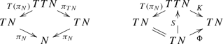
$$\begin{aligned} \Phi :T{\text {Imm}}^r(M,N)\rightarrow T{\text {Imm}}^r(M,N). \end{aligned}$$Here the condition \(p\ge 1\) is needed to ensure that the term \(P^{-1}\big (\bar{g}(Ph,h)\,{\text {Tr}}^g(\nabla Tf)\big )\) is again of regularity \(H^r\). The map \(\Phi \) corresponds uniquely to a \(C^\alpha \) spray S via the induced connection described in Lemma 2.6. In more detail: The right-hand side diagram in the proof of Sect. 2.5.(d) holds for any manifold N with connector K. Thus, replacing (N, K) by \(({\text {Imm}}^r(M,N),K_*)\), one obtains the diagram
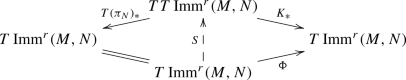
The spray S is \(C^\alpha \) because the connection \(K_*\) and the map \(\Phi \) are \(C^\alpha \). Therefore, by the theorem of Picard-Lindelöf, S admits a \(C^\alpha \) flow
$$\begin{aligned} {\text {Fl}}^S:U \rightarrow T{\text {Imm}}^{r}(M,N) \end{aligned}$$for a maximal open neighborhood U of \(\{0\}\times T{\text {Imm}}^r(M,N)\) in \({\mathbb {R}}\times T{\text {Imm}}^r(M,N)\). The neighborhood U is \({\text {Diff}}(M)\)-invariant thanks to the \({\text {Diff}}(M)\)-equivariance of S.
- (b):
-
follows from (a) as in [11, Theorem 6.6], and (c) follows from Lemma B.1 by writing \({\text {Imm}}(M,N)\) as the intersection of all \({\text {Imm}}^{r_0+k}(M,N)\) with \(k \in {\mathbb {N}}_{\ge 0}\).

\(\square \)
4.5 Corollary
Theorem 4.4 with \(\alpha =\omega \) remains valid if the assumptions in Sect. 4.1 are modified as follows: the metric \(\bar{g}\) is only \(C^\infty \), and the connection \(\nabla \) in condition (d) is replaced by an auxiliary connection \({\hat{\nabla }}\), which is induced by a torsion-free \(C^\omega \) connection on N, as described in Lemma 2.6.
Proof
In the proof of Theorem 4.3, the geodesic equation is derived by expressing the first variation \(\partial _s E\) of the energy functional using the Levi–Civita connection of \(\bar{g}\). If the auxiliary connection \({\hat{\nabla }}\) is used instead, then the following additional terms appear in the formula for \(\partial _s E\):
Accordingly, letting \(\Psi \) denote the right-hand side of the original geodesic equation with \(\nabla P\) replaced by \({\hat{\nabla }} P\), i.e.,
the geodesic equation becomes
One verifies as in the proof of Theorem 4.4 that the right-hand side, seen as a function of \(f_t\), is a fiber-wise quadratic real analytic map \(T{\text {Imm}}^r(M,N)\rightarrow T{\text {Imm}}^r(M,N)\). As the auxiliary connection \({\hat{\nabla }}\) is real analytic, this implies that the corresponding spray is real analytic, as well; see Sect. 2.5. Since the spray is independent of the auxiliary connection \({\hat{\nabla }}\), one may proceed as in the proof of Theorem 4.4. \(\square \)
The following theorem shows that (scale-invariant) fractional-order Sobolev metrics satisfy the conditions in Sect. 4.1. This implies local well-posedness of their geodesic equations by Theorem 4.4. Further metrics considered in the literature include curvature weighted metrics and the so-called general elastic metric [33], which can also be formulated in the present framework [12]. The proof takes advantage of the fact that the adjoint in the geodesic equation 4.3 has been split into normal and tangential parts. The normal part has the correct Sobolev regularity thanks to Lemma 3.2. The tangential part incurs a loss of derivatives, but the bad terms cancel out with some other terms in the geodesic equation as shown in part (a) of the proof of Theorem 4.3.
4.6 Theorem
The following operators satisfy the conditions in Sect. 4.1 with \(\alpha =\omega \) for any \(p \in [1,\infty )\) and \(r_0 \in ({\text {dim}}(M)/2+2,\infty )\cap [p+1,\infty )\):
Thus, the geodesic equations of these metrics are well posed in the sense of Theorem 4.4.
Proof
We will prove this result only for the first field of operators because the proof for the second one is analogous. We shall check conditions (a)–(d) of Sect. 4.1.
- (a):
follows from Lemma 3.1.
- (b):
\({\text {Diff}}(M)\)-equivariance of \((1+\Delta ^{f^*\bar{g}})\) is well-known for smooth f and follows in the general case by approximation, noting that the pull-back along a smooth diffeomorphism is a bounded linear map between Sobolev spaces of the same order of regularity [31, Theorem B.2]. As the functional calculus preserves commutation relations, this implies the \({\text {Diff}}(M)\)-equivariance of \((1+\Delta ^g)^p\).
- (c):
is well-known for smooth f, h, k and follows in the general case by approximation using the continuity of \(f\mapsto \langle \cdot ,\cdot \rangle _{H^0(f^*\bar{g})}\) established in [6, Lemma 3.3] and the continuity of \(f\mapsto P_f\).
- (d):
Recall from Lemma 3.2 that the derivative of \(P_f\) in normal directions extends to a real analytic map
$$\begin{aligned} H^{2p-r}_{{\text {Imm}}^r}(M,TN) \ni m \mapsto \big (h\mapsto {\hat{\nabla }}_{m^\bot }P_fh\big ) \in L(H^r_{{\text {Imm}}^r}(M,TN),H^{1-r}_{{\text {Imm}}^r}(M,TN)). \end{aligned}$$Equivalently, the following map is real analytic:
$$\begin{aligned} H^{r}_{{\text {Imm}}^r}(M,TN)= & {} T{\text {Imm}}^r(M,N) \ni h \mapsto \big (m\mapsto {\hat{\nabla }}_{m^\bot } P_f h\big )\\&\in L(H^{2p-r}_{{\text {Imm}}^r}(M,TN),H^{1-r}_{{\text {Imm}}^r}(M,N)). \end{aligned}$$Dualization using the \(H^0(g)\) duality shows that the adjoint is real analytic
$$\begin{aligned} T{\text {Imm}}^r(M,N) \ni h \mapsto {\text {Adj}}({\hat{\nabla }} P)(h,\cdot )^\bot \in L(H^{r-1}_{{\text {Imm}}^r}(M,TN),H^{r-2p}_{{\text {Imm}}^r}(M,TN)). \end{aligned}$$In particular, the adjoint is real analytic
$$\begin{aligned} T{\text {Imm}}^r(M,N) \ni h \mapsto {\text {Adj}}({\hat{\nabla }} P)(h,\cdot )^\bot \in L(H^r_{{\text {Imm}}^r}(M,TN),H^{r-2p}_{{\text {Imm}}^r}(M,TN)). \end{aligned}$$
\(\square \)
4.7 Remark
For Sobolev metrics of integer order \(p \in {\mathbb {N}}_{>0}\), condition (d) of Sect. 4.1 can be verified directly by a term-by-term investigation of the following explicit formula for the normal part of the adjoint [11, Section 8.2], assuming that \({\hat{\nabla }}=\nabla \) is the Levi–Civita connection of \(\bar{g}\):
Here \(g=f^*\bar{g}\), \(\Delta =\Delta ^{g}\), \(\nabla =\nabla ^g\), and \(R^{\bar{g}}\) denotes the curvature on \((N,\bar{g})\). This direct calculation is consistent with the more general argument of Theorem 4.6.
5 Special cases
This section describes several applications of the general well-posedness result, Theorem 4.4. First, we consider the geodesic equation of right-invariant Sobolev metrics on the diffeomorphism group \({\text {Diff}}(M)\). In Eulerian coordinates, this equation is called Euler–Arnold [2] or EPDiff [29] equation and reads as
In Lagrangian coordinates, the equation takes the form shown in the following corollary. The conditions for local well-posedness in this corollary agree with the ones in [3], where metrics governed by a general class of pseudo-differential operators are investigated. The proof is an application of Theorem 4.4 to \({\text {Diff}}(M)\), seen as an open subset of \({\text {Imm}}(M,M)\). Moreover, the proof extends Theorem 4.4 to lower Sobolev regularity using some cancellations which are due to the vanishing normal bundle. The notation is as in Theorem 4.4.
5.1 Corollary
Diffeomorphisms. A smooth curve \(\varphi :[0,1]\rightarrow {\text {Diff}}(M)\) is a critical point of the energy functional
if and only if it satisfies the geodesic equation
The geodesic equation is well-posed in the sense of Theorem 4.4 if P satisfies conditions (a)–(c) of Sect. 4.1 for some \(p \in [1/2,\infty )\) and all \(r\in [r_0,\infty )\) with \(r_0 \in ({\text {dim}}(M)/2+1,\infty )\). In particular, this is the case if \(P=(1+\Delta )^p\) with
\(p \in [1,\infty )\) and \(r \in ({\text {dim}}(M)/2+1,\infty )\cap [p+1,\infty )\); or
\(p \in [1/2,1)\) and \(r \in ({\text {dim}}(M)/2+1,\infty )\cap [p+3/2,\infty )\).
Proof
The formula for the geodesic equation follows from Theorem 4.3 because the terms \({\text {Adj}}(\nabla P)^\bot \) and \(\nabla Tf=(\nabla Tf)^\bot \) vanish. To show well-posedness of the geodesic equation, note that condition (d) of Sect. 4.1 is trivially satisfied because \({\text {Adj}}(\nabla P)^\bot \) vanishes. Moreover, note that the condition \(p \in [1,\infty )\) in Theorem 4.4 can be replaced by the weaker condition \(p \in [1/2,\infty )\) because the term \(\nabla Tf\), which is of second order in f, vanishes. This can be seen by a term-by-term investigation of the right-hand side of the geodesic equation as in the proof of Theorem 4.4. Therefore, the geodesic equation is well-posed for any operator field P satisfying conditions (a)–(c) of Sect. 4.1 for some \(p \in [1/2,\infty )\) and all \(r\in [r_0,\infty )\) with \(r_0 \in ({\text {dim}}(M)/2+1,\infty )\), as claimed.
It remains to verify these conditions for the specific operator \(P=(1+\Delta )^p\). Condition (a) for \(p\ge 1\) follows from Lemma 3.1, and condition (a) for \(p\in [1/2,1)\) is verified as follows. We split the operator \(P_\varphi \) in two components,
As \(1+p\ge 1\), Lemma 3.1 shows that the operator \((1+\Delta ^{\varphi ^*\bar{g}})^{1+p}\) is a real analytic section of the bundle
for any r such that \(r-2p-2\ge 1-r\), i.e., \(r\ge p+3/2\). Similarly, under even weaker conditions, the operator \((1+\Delta ^{\varphi ^*\bar{g}})^{-1}\) is a real analytic section of the bundle
By the chain rule, the operator \(P_\varphi \) is real analytic as required in condition (a). Conditions (b) and (c) can be verified as in the proof of Theorem 4.6. \(\square \)
Next we consider reparametrization-invariant Sobolev metrics on spaces of immersed curves, i.e., we consider the special case \(M=S^1\). Our interest in these spaces stems from their fundamental role in the field of mathematical shape analysis; see e.g. [7, 9, 36, 56, 62] for \({\mathbb {R}}^n\)-valued curves and [18, 42, 54, 55] for manifold-valued curves. For curves in \({\mathbb {R}}^n\) local well-posedness of the geodesic equation for integer-order metrics has been shown in [47]. This has recently been extended to fractional-order metrics in [8]. The following corollary of our main result further generalizes this to fractional-order metrics on spaces of manifold-valued curves:
5.2 Corollary
Curves. A smooth curve \(c :[0,1]\rightarrow {\text {Imm}}(S^1,N)\) is a critical point of the energy functional
if and only if it satisfies the geodesic equation
where \(\partial _s=|c_{\theta }|^{-1}\partial _{\theta }\) denotes the normalization of the coordinate vector field \(\partial _{\theta }\), \(v_c={\partial _s}c\) the unit-length tangent vector, and \(H_c=(\nabla _{\partial _s} v_c)^{\bot }\) the vector-valued curvature of c.
If the operator P satisfies the conditions of Sect. 4.1 for some \(p \in [1,\infty )\) and all \(r\in [r_0,\infty )\) with \(r_0 \in ({\text {dim}}(M)/2+1,\infty )\), then the geodesic equation is well-posed in the sense of Theorem 4.4. This is in particular the case for the operator \(P=(1-\nabla _{\partial _s}\nabla _{\partial _s})^p\) if \(p \in [1,\infty )\) and \(r \in ({\text {dim}}(M)/2+1,\infty )\cap [p+1,\infty )\).
Proof
This follows directly from Theorems 4.3, 4.4 and 4.6. \(\square \)
The last special case to be discussed in this section is \(N=\mathbb R^n\), which includes in particular the space of surfaces in \(\mathbb R^3\). In the article [11] we proved a local well-posedness result for integer-order metrics. The proof given there had a gap, which has been corrected in the article [50]. The following corollary of our main result extends this to fractional order metrics:
5.3 Corollary
Flat ambient space. A smooth curve \(f :[0,1]\rightarrow {\text {Imm}}(M,\mathbb R^n)\) is a critical point of the energy functional
if and only if it satisfies the geodesic equation
where \(\langle \cdot ,\cdot \rangle \) denotes the Euclidean scalar product on \({\mathbb {R}}^n\), \(g=f^*\langle \cdot ,\cdot \rangle \) the induced pullback metric on M, and \(H_f={\text {Tr}}^g(d^2f)^{\bot }\) the vector-valued mean curvature of f.
If the operator P satisfies the conditions of Sect. 4.1 for some \(p \in [1,\infty )\) and all \(r\in [r_0,\infty )\) with \(r_0 \in ({\text {dim}}(M)/2+1,\infty )\), then the geodesic equation is well-posed in the sense of Theorem 4.4. This is in particular the case for the operator \(P=(1+\Delta )^p\) with \(p \in [1,\infty )\) and \(r \in ({\text {dim}}(M)/2+1,\infty )\cap [p+1,\infty )\).
Proof
This follows from Theorems 4.3, 4.4, and 4.6 with \(N={\mathbb {R}}^n\), noting that the covariant derivative on \({\mathbb {R}}^n\) and the induced covariant derivative on \({\text {Imm}}^r(M,{\mathbb {R}}^n)\) coincide with ordinary derivatives. \(\square \)
References
Arbogast, L.F.A.: Du calcul des dérivations. Levrault, Strasbourg (1800)
Arnold, V.I.: Sur la géométrie différentielle des groupes de Lie de dimension infinie et ses applications à l’hydrodynamique des fluides parfaits. Ann. Inst. Fourier (Grenoble), 16(fasc. 1), 319–361 (1966)
Bauer, M., Bruveris, M., Cismas, E., Escher, J., Kolev, B.: Well-posedness of the EPDiff equation with a pseudo-differential inertia operator. To appear in J. Differ. Equ. (2020). https://doi.org/10.1016/j.jde.2019.12.008
Bauer, M., Bruveris, M., Harms, P., Michor, P.W.: Vanishing geodesic distance for the Riemannian metric with geodesic equation the KdV-equation. Ann. Glob. Anal. Geom. 41(4), 461–472 (2012)
Bauer, M., Bruveris, M., Harms, P., Michor, P.W.: Geodesic distance for right invariant Sobolev metrics of fractional order on the diffeomorphism group. Ann. Glob. Anal. Geom. 44(1), 5–21 (2013)
Bauer, M., Bruveris, M., Harms, P., Michor, P.W.: Smooth perturbations of the functional calculus and applications to Riemannian geometry on spaces of metrics (2018). arXiv:1810.03169
Bauer, M., Bruveris, M., Harms, P., Møller-Andersen, J.: A numerical framework for Sobolev metrics on the space of curves. SIAM J. Imaging Sci. 10(1), 47–73 (2017)
Bauer, M., Bruveris, M., Kolev, B.: Fractional Sobolev metrics on spaces of immersed curves. Calc. Var. Partial. Differ. Equ. 57(1), 27 (2018)
Bauer, M., Bruveris, M., Michor, P.W.: Overview of the geometries of shape spaces and diffeomorphism groups. J. Math. Imaging Vis. 50(1–2), 60–97 (2014)
Bauer, M., Escher, J., Kolev, B.: Local and global well-posedness of the fractional order EPDiff equation on \(\mathbb{R}^d\). J. Differ. Equ. 258(6), 2010–2053 (2015)
Bauer, M., Harms, P., Michor, P.W.: Sobolev metrics on shape space of surfaces. J. Geom. Mech. 3(4), 389–438 (2011)
Bauer, M., Harms, P., Michor, P.W.: Sobolev metrics on shape space, II: weighted Sobolev metrics and almost local metrics. J. Geom. Mech. 4(4), 365–383 (2012)
Bauer, M., Harms, P., Preston, S.C.: Vanishing distance phenomena and the geometric approach to SQG. Arch. Ration. Mech. Anal. 235, 1445–1466 (2020). https://doi.org/10.1007/s00205-019-01449-7
Bauer, M., Kolev, B., Preston, S.C.: Geometric investigations of a vorticity model equation. J. Differ. Equ. 260(1), 478–516 (2016)
Behzadan, A., Holst, M.: On certain geometric operators between Sobolev spaces of sections of tensor bundles on compact manifolds equipped with rough metrics (2017). arXiv:1704.07930
Bruveris, M.: Regularity of maps between Sobolev spaces. Ann. Glob. Anal. Geom. 52(1), 11–24 (2017)
Camassa, R., Holm, D.D.: An integrable shallow water equation with peaked solitons. Phys. Rev. Lett. 71(11), 1661 (1993)
Celledoni, E., Eidnes, S., Schmeding, A.: Shape analysis on homogeneous spaces: a generalised SRVT framework. In: The Abel Symposium. Springer, pp. 187–220 (2016)
Constantin, P., Lax, P.D., Majda, A.: A simple one-dimensional model for the three-dimensional vorticity equation. Commun. Pure Appl. Math. 38(6), 715–724 (1985)
Constantin, P., Majda, A.J., Tabak, E.: Formation of strong fronts in the 2-D quasigeostrophic thermal active scalar. Nonlinearity 7(6), 1495 (1994)
Conway, J.B.: A Course in Functional Analysis, vol. 96. Springer, Berlin (2013)
Defant, A., Floret, K.: Tensor Norms and Operator Ideals, vol. 176. Elsevier, Amsterdam (1992)
Ebin, D.G., Marsden, J.E.: Groups of diffeomorphisms and the motion of an incompressible fluid. Ann. Math. 92, 102–163 (1970)
Escher, J., Kolev, B.: Right-invariant Sobolev metrics of fractional order on the diffeomorphism group of the circle. J. Geom. Mech. 6(3), 335–372 (2014)
Faà di Bruno, C.F.: Note sur une nouvelle formule du calcul différentielle. Q. J. Math. 1, 359–360 (1855)
Frölicher, A., Kriegl, A.: Linear Spaces and Differentiation Theory. Pure and Applied Mathematics (New York). Wiley, Chichester (1988)
Grenander, U., Miller, M.I.: Computational anatomy: an emerging discipline. Q. Appl. Math. 56(4), 617–694 (1998)
Große, N., Schneider, C.: Sobolev spaces on Riemannian manifolds with bounded geometry: general coordinates and traces. Math. Nachr. 286(16), 1586–1613 (2013)
Holm, D.D., Marsden, J.E.: Momentum maps and measure-valued solutions (peakons, filaments, and sheets) for the EPDiff equation. In: The Breadth of Symplectic and Poisson Geometry, volume 232 of Progress in Mathematics. Birkhäuser Boston, Boston, MA, pp. 203–235 (2005)
Hunter, J.K., Saxton, R.: Dynamics of director fields. SIAM J. Appl. Math. 51(6), 1498–1521 (1991)
Inci, H., Kappeler, T., Topalov, P.: On the regularity of the composition of diffeomorphisms. Mem. Am. Math. Soc. 226(1062):vi+60 (2013)
Jarchow, H.: Locally Convex Spaces. Springer, Berlin (2012)
Jermyn, I., Kurtek, S., Laga, H., Srivastava, A.: Elastic shape analysis of three-dimensional objects. Synth. Lect. Comput. Vis. 12, 1–185 (2017)
Jerrard, R.L., Maor, C.: Vanishing geodesic distance for right-invariant Sobolev metrics on diffeomorphism groups. Ann. Glob. Anal. Geom. 55(4), 631–656 (2019)
Khesin, B., Wendt, R.: The geometry of infinite-dimensional groups, vol. 51. Springer, Berlin (2008)
Klassen, E., Srivastava, A., Mio, M., Joshi, S.H.: Analysis of planar shapes using geodesic paths on shape spaces. IEEE Trans. Pattern Anal. Mach. Intell. 26(3), 372–383 (2004)
Kolář, I., Michor, P.W., Slovák, J.: Natural Operations in Differential Geometry. Springer, Berlin (1993)
Kolev, B.: Local well-posedness of the EPDiff equation: a survey. J. Geom. Mech. 9(2), 167–189 (2017)
Kouranbaeva, S.: The Camassa–Holm equation as a geodesic flow on the diffeomorphism group. J. Math. Phys. 40(2), 857–868 (1999)
Kriegl, A., Michor, P.W.: Product preserving functors of infinite-dimensional manifolds. Arch. Math. (Brno) 32(4), 289–306 (1996)
Kriegl, A., Michor, P.W.: The Convenient Setting of Global Analysis. Mathematical Surveys and Monographs, vol. 53. American Mathematical Society, Providence (1997)
Le Brigant, A.: Computing distances and geodesics between manifold-valued curves in the SRV framework. J. Geom. Mech. 9(2), 131–156 (2017)
Lenells, J.: The Hunter–Saxton equation describes the geodesic flow on a sphere. J. Geom. Phys. 57(10), 2049–2064 (2007)
Marsden, J.E., Ratiu, T., Weinstein, A.: Semidirect products and reduction in mechanics. Trans. Am. Math. Soc. 281(1), 147–177 (1984)
Michor, P.W.: Topics in Differential Geometry. Graduate Studies in Mathematics, vol. 93. American Mathematical Society, Providence (2008)
Michor, P.W.: Manifolds of mappings for continuum mechanics. In Geometric Continuum Mechanics—An Overview. Birkhauser, pp. 1–60 (2020)
Michor, P.W., Mumford, D.: An overview of the Riemannian metrics on spaces of curves using the Hamiltonian approach. Appl. Comput. Harmon. Anal. 23(1), 74–113 (2007)
Misiołek, G.: A shallow water equation as a geodesic flow on the Bott–Virasoro group. J. Geom. Phys. 24(3), 203–208 (1998)
Misiołek, G., Preston, S.C.: Fredholm properties of Riemannian exponential maps on diffeomorphism groups. Invent. Math. 179(1), 191 (2010)
Müller, O.: Applying the index theorem to non-smooth operators. J. Geom. Phys. 116, 140–145 (2017)
Ovsienko, V.Y., Khesin, B.A.: Korteweg–de Vries superequation as an Euler equation. Funct. Anal. Appl. 21(4), 329–331 (1987)
Shnirel’man, A.I.: On the geometry of the group of diffeomorphisms and the dynamics of an ideal incompressible fluid. Math. USSR Sbornik 56(1), 79 (1987)
Srivastava, A., Klassen, E.: Functional and Shape Data Analysis. Springer, New York (2016). https://doi.org/10.1007/978-1-4939-4020-2
Su, J., Kurtek, S., Klassen, E., Srivastava, A., et al.: Statistical analysis of trajectories on Riemannian manifolds: bird migration, hurricane tracking and video surveillance. Ann. Appl. Stat. 8(1), 530–552 (2014)
Su, Z., Klassen, E., Bauer, M.: Comparing curves in homogeneous spaces. Differ. Geom. Appl. 60, 9–32 (2018)
Sundaramoorthi, G., Mennucci, A., Soatto, S., Yezzi, A.: A new geometric metric in the space of curves, and applications to tracking deforming objects by prediction and filtering. SIAM J. Imaging Sci. 4(1), 109–145 (2011)
Treves, F.: Topological Vector Spaces, Distributions and Kernels: Pure and Applied Mathematics. Academic Press, New York (1967)
Triebel, H.: Theory of Function Spaces II. Monographs in Mathematics, vol. 84. Birkhäuser, Boston (1992)
Vishik, S., Dolzhanskii, F.: Analogs of the Euler–Lagrange equations and magnetohydrodynamics equations related to Lie groups. Sov. Math. Dokl. 19, 149–153 (1978)
Washabaugh, P.: The SQG equation as a geodesic equation. Arch. Ration. Mech. Anal. 222(3), 1269–1284 (2016)
Wunsch, M.: On the geodesic flow on the group of diffeomorphisms of the circle with a fractional Sobolev right-invariant metric. J. Nonlinear Math. Phys. 17(1), 7–11 (2010)
Younes, L.: Computable elastic distances between shapes. SIAM J. Appl. Math. 58(2), 565–586 (1998)
Younes, L.: Shapes and Diffeomorphisms, vol. 171. Springer, Berlin (2010)
Acknowledgements
Open access funding provided by University of Vienna.
Author information
Authors and Affiliations
Corresponding author
Additional information
Communicated by J. Jost.
Publisher's Note
Springer Nature remains neutral with regard to jurisdictional claims in published maps and institutional affiliations.
We thank Martins Bruveris, Boris Kolev, Andreas Kriegl, Peer Kunstmann, and Lutz Weis for helpful discussions. Moreover, we gratefully acknowledge support in the form of a Research in Teams stipend of the Erwin Schrödinger Institute Vienna. MB was partially supported by NSF-Grant 1912037 (collaborative research in connection with NSF-Grant 1912030). PH was partially supported in the form of a Junior Fellowship of the Freiburg Institute of Advanced Studies.
Appendices
Appendix A: The push-forward operator on Sobolev spaces
A.1 Theorem
Smooth curves in convenient vector spaces. [26, 4.1.19] Let \(c:{\mathbb {R}}\rightarrow E\) be a curve in a convenient vector space E. Let \({\mathcal {V}}\subset E'\) be a subset of bounded linear functionals such that the bornology of E has a basis of \(\sigma (E,{\mathcal {V}})\)-closed sets. Then the following are equivalent:
- (a):
c is smooth
- (b):
For each \(k\in {\mathbb {N}}\) there exists a locally bounded curve \(c^{k}:{\mathbb {R}}\rightarrow E\) such that for each \(\ell \in {\mathcal {V}}\) the function \(\ell \circ c\) is smooth \({\mathbb {R}}\rightarrow {\mathbb {R}}\) with \((\ell \circ c)^{(k)}=\ell \circ c^{k}\).
If E is reflexive, then for any point separating subset \({\mathcal {V}}\subset E'\) the bornology of E has a basis of \(\sigma (E,{\mathcal {V}})\)-closed subsets, by [26, 4.1.23].
This theorem is surprisingly strong: Note that \({\mathcal {V}}\) does not need to recognize bounded sets. We shall use the theorem in situations where \({\mathcal {V}}\) is just the set of all point evaluations on suitable Sobolev spaces.
A.2 Lemma
Smooth curves in Sobolev spaces of sections. Let E be a vector bundle over M, and let \(\nabla \) be a connection on E. Then it holds for each \(r\in ({\text {dim}}(M)/2,\infty )\) that the space \(C^\infty (\mathbb R,\Gamma _{H^r}(E))\) of smooth curves in \(\Gamma _{H^r}(E)\) consists of all continuous mappings \(c:{\mathbb {R}}\times M \rightarrow E\) with \(p\circ c = {\text {pr}}_2:{\mathbb {R}}\times M\rightarrow M\) such that:
For each \(x\in M\) the curve \(t\mapsto c(t,x)\in E_x\) is smooth; let \((\partial ^p_t c)(t,x) = \partial _t^p(c(t,x))\), and
For each \(p\in {\mathbb {N}}_{\ge 0}\), the curve \(\partial _t^pc\) has values in \(\Gamma _{H^r}(E)\) so that \(\partial _t^pc :{\mathbb {R}}\rightarrow \Gamma _{H^r}(E)\), and \(t \mapsto \Vert \partial _t c(t,\quad )\Vert _{H^r}\) is bounded, locally in t.
Proof
To see this we first choose a second vector bundle \(F\rightarrow M\) such that \(E\oplus _M F\) is a trivial bundle, i.e., isomorphic to \(M\times {\mathbb {R}}^n\) for some \(n\in {\mathbb {N}}\). Then \(\Gamma _{H^r}(E)\) is a direct summand in \(H^r(M,{\mathbb {R}}^n)\), so that we may assume without loss that E is a trivial bundle, and then, that it is 1-dimensional. So we have to identify \(C^\infty (\mathbb R,H^r(M,{\mathbb {R}}))\). But in this situation we can just apply Theorem A.1 for the set \({\mathcal {V}}\subset H^s(M,\mathbb R)'\) consisting just of all point evaluations \({\text {ev}}_x:H^r(M,{\mathbb {R}})\rightarrow {\mathbb {R}}\). \(\square \)
A.3 Lemma
Function spaces of mixed smoothness. Let U be an open subset of a finite-dimensional vector space, let \(r \in ({\text {dim}}(M)/2,\infty )\), let \(\alpha \in \{\infty ,\omega \}\), and let \(C^\alpha (U)=\varprojlim _p E_p\) be the representation of the complete locally convex space \(C^\alpha (U)\) as a projective limit of Banach spaces \(E_p\). Then
where \({\hat{\otimes }}\) is the injective, projective, or bornological tensor product, or any tensor product in-between, and where \(H^r(M,C^\alpha (U))\) is defined as the projective limit \(\varprojlim _p H^r(M,E_p)\).
The lemma justifies the following notation, which shall be used in Lemma A.5 below. If \(E_1\) and \(E_2\) are vector bundles over M, and \(U \subseteq E_1\) is an open neighborhood of the image of an \(H^r\) section, then we write \(\Gamma _{H^r}(C^\alpha (U,E_2))\) for the set of all fiber-preserving functions \(F:U \rightarrow E_2\) which have regularity \(H^rC^\alpha \) in every \(C^\alpha \) vector bundle chart of \(E_1\). Loosely speaking, these are sections of regularity \(H^r\) in the foot point and regularity \(C^\alpha \) in the fibers.
Proof
The space \(C^\infty (U)\) is nuclear by [57, Corollary to Theorem 51.4], and the space \(C^\omega (U)\) is nuclear as a countable inductive limit of nuclear spaces of holomorphic functions [41, Theorem 30.11]. Let \(\otimes _\varepsilon \), \(\otimes _\pi \), and \(\otimes _\beta \) be the injective, projective, and bornological completed tensor products, respectively. Then
where the first equality holds because \(C^\alpha (U)\) is nuclear, and the second equality holds by [41, Proposition 5.8] using that \(H^r(M)\) is a normed space, and \(C^\omega (V)\) is an (LF)-space and therefore bornological. Thus, all tensor spaces \(C^\alpha (U){\hat{\otimes }} H^r(M)\) are equal. Moreover,
by [57, Theorem 44.1], and
by [32, Corollary 16.7.5], where \({\mathcal {H}}\) denotes holomorphic functions and \({\tilde{U}}\) are open neighborhoods of U in the complexification of the underlying vector space. Let \(\Delta _2\) be the natural norm on \(L^2\) functions [22, 7.1]. Then
where the first equality holds because \(\varepsilon \le \Delta _2\le \pi \) [22, 7.1], the second one by the definition of tensor products of locally convex spaces [22, 35.2], and the third one because the fractional Laplacian \((1+\Delta ^g):H^r(M)\rightarrow L^2(M)\) with respect to any auxiliary Riemannian metric \(g \in {\text {Met}}(M)\) is an isometry and because \(L^2(M,E_p)=L^2(M)\otimes _{\Delta _2}E_p\) by the definition of \(\Delta _2\) [22, 7.2]. \(\square \)
A.4 Lemma
Push-forward of functions. Let U be an open subset of \({\mathbb {R}}\), and let \(r \in ({\text {dim}}(M)/2,\infty )\). Then \(H^r(M,U)\) is open in \(H^r(M,{\mathbb {R}})\), and the following statements hold.
- (a):
The following map is smooth:
$$\begin{aligned} H^rC^\infty (M\times U) \times H^r(M,U) \ni (F,h) \mapsto F\circ ({\text {Id}}_M,h) \in H^r(M). \end{aligned}$$- (b):
The following map is real analytic:
$$\begin{aligned} H^rC^\omega (M\times U) \times H^r(M,U) \ni (F,h) \mapsto F\circ ({\text {Id}}_M,h) \in H^r(M). \end{aligned}$$
Proof
The set \(\Gamma _{H^r}(U)\) is open in \(\Gamma _{H^r}(E_1)\) because \(\Gamma _{H^r}(E_1)\) is continuously included in \(\Gamma _{C}(E_1)\) thanks to the Sobolev embedding theorem.
- (a):
follows from the more general statement Lemma A.5.(a).
- (b’):
As an intermediate step, we claim that the following map is real analytic:
$$\begin{aligned} C^\omega (U) \times H^r(M,U) \ni (f,h) \mapsto f\circ h \in H^r(M). \end{aligned}$$For any \(f \in C^\omega (U)\) and \(h \in H^r(M,U)\), the composition \(f\circ h\) coincides with the Riesz functional calculus f(h), which is defined as follows [21, Theorem 4.7]. As the spectrum \(\sigma (h)\) equals the range of h, which is a compact subset of U, there is a set of positively oriented curves \(\Gamma =\{\gamma _1,\dots ,\gamma _n\}\) in \(U \setminus \sigma (h)\) such that \(\sigma (h)\) is inside of \(\Gamma \), and \({\mathbb {C}}\setminus U\) is outside of \(\Gamma \) [21, Proposition 4.4]. Then one defines f(h) as the following Bochner integral over the resolvent of h:
$$\begin{aligned} f(h) = \frac{-1}{2\pi \mathrm {i} }\int _\Gamma f(\lambda ) (h-\lambda )^{-1} d\lambda \end{aligned}$$For any fixed \(\Gamma \), this integral is well-defined and real analytic as claimed.
- (b):
The following map is real analytic thanks to (b’) and the boundedness of multiplication \(H^r(M)\times H^r(M)\rightarrow H^r(M)\):
$$\begin{aligned} H^r(M) \times C^\omega (U) \times H^r(M,U) \ni (a,f,h) \mapsto (a\otimes f)\circ ({\text {Id}}_M,h) \in H^r(M), \end{aligned}$$where \((a\otimes f)\circ ({\text {Id}}_M,h)\) denotes the map \(x \mapsto a(x)f(h(x))\). Equivalently, by the real analytic exponential law [41, 11.18], the following map is real analytic:
$$\begin{aligned} H^r(M) \times C^\omega (U) \ni (a,f) \mapsto \big (h \mapsto (a\otimes f)\circ ({\text {Id}}_M, h)\big ) \in C^\omega (H^r(M,U),H^r(M)). \end{aligned}$$This map is bilinear and real analytic, and therefore bounded. By the universal property of the bornological tensor product \(\otimes _\beta \) [41, 5.7], it descends to a bounded linear map
$$\begin{aligned} H^r(M) \otimes _\beta C^\omega (U) \ni F \mapsto \big (h \mapsto F\circ ({\text {Id}}_M,h)\big ) \in C^\omega (H^r(M,U),H^r(M)). \end{aligned}$$The domain of this map equals \(H^rC^\omega (M\times U)\) by Lemma A.3.
\(\square \)
A.5 Lemma
Push-forward of sections. Let \(E_1,E_2\) be vector bundles over M, let \(U\subset E_1\) be an open neighborhood of the image of a smooth section, let \(F:U\rightarrow E_2\) be a fiber preserving function, and let \(r \in ({\text {dim}}(M)/2,\infty )\). Then \(\Gamma _{H^r}(U)\) is open in \(\Gamma _{H^r}(E_1)\), and the following statements hold:
- (a):
If F is smooth or belongs to \(\Gamma _{H^r}(C^\infty (U,E_2))\), then the push-forward \(F_*\) is smooth:
$$\begin{aligned} F_*:\Gamma _{H^r}(U) \rightarrow \Gamma _{H^r}(E_2),\quad h\mapsto F\circ h. \end{aligned}$$- (b):
If F is real analytic or belongs to \(\Gamma _{H^r}(C^\omega (U,E_2))\), then the pushforward \(F_*\) is real analytic.
The notation \(\Gamma _{H^r}(C^\infty (U,E_2))\) and \(\Gamma _{H^r}(C^\omega (U,E_2))\) is explained in “Section A.3”.
Proof
- (a):
-
Let \(c:{\mathbb {R}}\ni t\mapsto c(t,\cdot )\in \Gamma _{H^r}(U)\) be a smooth curve. As \(r>{\text {dim}}(M)/2\), it holds for each \(x\in M\) that the mapping \({\mathbb {R}}\ni t \mapsto F_x(c(t,x))\in (E_2)_x\) is smooth. By the Faà di Bruno formula (see [25] for the 1-dimensional version, preceded in [1] by 55 years), we have for each \(p\in {\mathbb {N}}_{>0}\), \(t \in {\mathbb {R}}\), and \(x \in M\) that
$$\begin{aligned} \partial _t^p F_x (c(t,x)) = \sum _{j\in {\mathbb {N}}_{>0}} \sum _{\begin{array}{c} \alpha \in {\mathbb {N}}_{>0}^j\\ \alpha _1+\dots +\alpha _j =p \end{array}} \frac{1}{j!}d^j (F_x) (c(t,x))\Big ( \frac{\partial _t^{(\alpha _1)}c(t,x)}{\alpha _1!},\dots , \frac{\partial _t^{(\alpha _j)}c(t,x)}{\alpha _j!}\Big )\,. \end{aligned}$$For each \(x\in M\) and \(\alpha _x\in (E_2)_x^*\) the mapping \(s\mapsto \langle s(x),\alpha _x\rangle \) is a continuous linear functional on the Hilbert space \(\Gamma _{H^r}(E_2)\). The set \({\mathcal {V}}_2\) of all of these functionals separates points and therefore satisfies the condition of Theorem A.1. We also have for each \(p\in {\mathbb {N}}_{>0}\), \(t \in {\mathbb {R}}\), and \(x \in M\) that
$$\begin{aligned} \partial _t^p\langle F_x (c(t,x)),\alpha _x\rangle&= \langle \partial _t^p F_x (c(t,x)),\alpha _x\rangle . \end{aligned}$$Using the explicit expressions for \(\partial _t^p F_x (c(t,x))\) from above we may apply Lemma A.2 to conclude that \(t\mapsto F(c(t,\;))\) is a smooth curve \({\mathbb {R}}\rightarrow \Gamma _{H^r}(E_2)\). Thus, \(F_*\) is a smooth mapping, and we have shown (a).
- (b’):
-
We claim that (b) holds when F is fiber-wise linear. Then F can be identified with a map in \(\check{F} \in \Gamma _{H^r}(L(E_1,E_2))\). For any \(h \in \Gamma _{H^r}(E_1)\), the composition \(F\circ h\) equals the trace \(\check{F}.h\), which is real analytic in h by the module properties 2.3.
- (b):
-
To prove the general case, we write \(E_1\) and \(E_2\) as sub-bundles of a trivial bundle \(M\times V\). The corresponding inclusion and projection mappings are real analytic mappings of vector bundles and are denoted by
$$\begin{aligned} i_1&:E_1 \rightarrow M\times V,&i_2&:E_2 \rightarrow M\times V,&\pi _1&:M\times V\rightarrow E_1,&\pi _2&:M\times V\rightarrow E_2. \end{aligned}$$Then the set \({\tilde{U}} := \pi _1^{-1}(U)\subseteq M\times V\) and the map \({\tilde{F}}:=i_2\circ F\circ \pi _1\) fit into the following commutative diagrams:

All maps in the diagram on the left are real analytic by definition. The map \(({\tilde{F}})_*\) is real analytic by Lemma A.4.(b) applied component-wise to the trivial bundle \(M\times V\), and the maps \((i_1)_*\) and \((\pi _2)_*\) are real analytic by (b’). Therefore, \(F_*=(\pi _2)_*\circ ({\tilde{F}})_*\circ (i_1)_*\) is real analytic, which proves (b).

\(\square \)
Appendix B: A real analytic no-loss no-gain result
The following lemma is a variant of the no-loss-no-gain theorem of Ebin and Marsden [23], adapted to the real analytic sprays on spaces of immersions as in the setting of Theorem 4.4. The proof is a minor adaptation of the proof in [23]; see also [16].
B.1 Lemma
Real analytic no-loss no-gain. Let \(r_0>{\text {dim}}(M)/2+1\) and let \(\alpha \in \{\infty ,\omega \}\). For each \(r\ge r_0\), let \(S^r\) be a \({\text {Diff}}(M)\)-invariant \(C^\alpha \) vector field on \(T{\text {Imm}}^r(M,N)\) such that \(Ti_{r,s} \circ S^r = S^s \circ i_{r,s}\) where \(i_{r,s}:T{\text {Imm}}^r(M,N)\rightarrow T{\text {Imm}}^s(M,N)\) is the \(C^\alpha \)-embedding for \(r_0\le s<r\). By the theorem of Picard-Lindelöf each \(S^r\) has a maximal \(C^\alpha \)-flow \({\text {Fl}}^{S^r}:U^r \rightarrow T{\text {Imm}}^r(M,N)\) for an open neighborhood \(U^r\) of \(\{0\}\times T{\text {Imm}}^r(M,N)\) in \({\mathbb {R}}\times T{\text {Imm}}^r(M,N)\).
Then \(U^r = U^s\cap ( {\mathbb {R}}\times T{\text {Imm}}^r(M,N))\) for all \(r_0+1 \le r\) and \(r_0\le s\le r\). Thus, there is no loss or gain in regularity during the evolution along any \(S^r\) for \(r\ge r_0+1\).
Proof
- (a):
-
We shall use the following result [23, Lemma 12.2]: Any\(h\in H^r(M,TN)\)such that\(Th\circ X\in H^r(M,TTN)\)for all\(X\in {\mathfrak {X}}(M)\)satisfies\(h\in H^{r+1}(M,TN)\).
- (b):
-
For \(h\in T{\text {Imm}}^r(M,N)\) let \(J^r_h\) be the open interval such that \(U^r\cap ({\mathbb {R}}\times \{h\}) = J^r_h\times \{h\}\), i.e., \(J^r_h\) is the maximal domain of the integral curve of \(S^r\) through h in \(T{\text {Imm}}^r(M,N)\); see [41, 32.14]. Since \(i_{r,s}\circ {\text {Fl}}^{S^r}_t = {\text {Fl}}^{S^s}_t\circ \) (see [41, 32.16]), for \(h\in T{\text {Imm}}^r(M,N)\) we have \(J^r_h\subseteq J^s_h\) for \(r_0\le s<r\).
- (c):
-
Claim.For\(h\in T{\text {Imm}}^{r+1}(M,N)\)we have\(J^r_h = J^{r+1}_h\).
Since \(S^r\) is invariant under the pullback action of \({\text {Diff}}(M)\), we have for \(h\in T{\text {Imm}}^{r+1}(M,N)\) and any \(X\in {\mathfrak {X}}(M)\) that
$$\begin{aligned} {\text {Fl}}^{S^r}_t(h\circ {\text {Fl}}^X_u) = {\text {Fl}}^{S^r}_t(h) \circ {\text {Fl}}^X_u\,. \end{aligned}$$Differentiating both side we get
$$\begin{aligned} T({\text {Fl}}^{S^r}_t(h))\circ X&= \partial _u|_0 ( {\text {Fl}}^{S^r}_t(h) \circ {\text {Fl}}^X_u) = \partial _u|_0 ({\text {Fl}}^{S^r}_t(h\circ {\text {Fl}}^X_u)) \\&= T({\text {Fl}}^{S^r}_t)(\partial _u|_0(h\circ {\text {Fl}}^X_u)) = T({\text {Fl}}^{S^r}_t)(Th\circ X) \end{aligned}$$Since \(Th\circ X \in H^r(M,TTN)\) we see that \(T({\text {Fl}}^{S^r}_t(h))\circ X \in H^r(M,TTN)\). By result (a) we get \({\text {Fl}}^{S^r}_t(h)\in T{\text {Imm}}^{r+1}(M,N)\), and thus \(J^{r}_h\supseteq J^{r+1}_h\). The converse inclusion is (b).
- (d):
-
Let \(r_0+1\le s< r<s+1\) and let \(h\in T{\text {Imm}}^{r}(M,N)\). Then
$$\begin{aligned} J^r_h \subseteq J^s_h\subseteq J^{r-1}_h= J^r_h, \end{aligned}$$where the inclusions follow from (b), (b), and (c) , respectively. Thus we have \(J^r_h=J^s_h=J^{r-1}_h\).\(\square \)
Rights and permissions
Open Access This article is licensed under a Creative Commons Attribution 4.0 International License, which permits use, sharing, adaptation, distribution and reproduction in any medium or format, as long as you give appropriate credit to the original author(s) and the source, provide a link to the Creative Commons licence, and indicate if changes were made. The images or other third party material in this article are included in the article’s Creative Commons licence, unless indicated otherwise in a credit line to the material. If material is not included in the article’s Creative Commons licence and your intended use is not permitted by statutory regulation or exceeds the permitted use, you will need to obtain permission directly from the copyright holder. To view a copy of this licence, visit http://creativecommons.org/licenses/by/4.0/.
About this article

Cite this article
Bauer, M., Harms, P. & Michor, P.W. Fractional Sobolev metrics on spaces of immersions. Calc. Var. 59, 62 (2020). https://doi.org/10.1007/s00526-020-1719-5
Received:
Accepted:
Published:
DOI: https://doi.org/10.1007/s00526-020-1719-5