
Abstract
Quantifying the trajectory similarity is a fundamental functionality in analysis tasks of spatio-temporal data. Existing classic methods compute the trajectory similarity based on point matching, which are unable to cope with low-quality trajectories (e.g., have non-uniform sampling rates or noise points), especially when we take both spatial coordinates and the time components into account. While some studies with deep learning methods exist, they did not consider the time components of trajectories and the robustness of similarity measure simultaneously, thus they fail to retrieve similarity-based queries in spatio-temporal databases where time components of trajectories are also important. In practice, the time-aware trajectory similarity computation can be better applied to diverse scenarios, yet the time complexity also heavily increases. To enable efficient and robust similarity computation on massive-scale trajectories, we developed a novel RSTS model based on deep representation learning, in which we take the time components into account. Extensive experiments show that our proposal constantly outperforms another two methods, and the similarity measure based on our RSTS model is robust to low-quality trajectories.
1 Introduction
With the continued growth of location-tracking devices (e.g., vehicle navigation systems and smart phones) and GPS-enabled services (e.g., Google Maps), the volume of trajectory data is skyrocketing. Trajectory similarity measurement, as one of the fundamental functionalities in spatio-temporal data analytics, has been extensively investigated by existing literature. A host of methods have been proposed [1,2,3,4] to measure trajectory similarity in diverse application scenarios.
Existing methods generally assume that the sampled trajectories have a uniform and consistent sampling rate. Two trajectories are considered to be similar if they can form a pairwise matching for the majority of their sample points. However, sampling rates vary among location-tracking devices [5] due to various reasons, including but not limited to battery constrains, intermittent signal disruptions, and system settings. In such cases, matching-based methods are proved to be ineffective. To tackle it, EDwP [3] was proposed to match trajectories through dynamic interpolation to cope with this issue. However, in most cases, trajectories are of non-uniform sampling rates, as well as other low-quality characters. We proceed to illustrate a toy example of exact moving route, high-quality trajectory, and low-quality trajectory of a moving object. Given a moving object o, we let Ra be a exact moving route of o during a period of time, which is a curve that records the continuous locations traveled by the object. We let a high-quality trajectory of exact moving route Ra be a sequence of sampled points with high frequency. And we let a low-quality trajectory of exact moving route Ra be a sequence of sampled points with low frequency, as well as some noisy location points are included. Compared to the low-quality trajectory, the high-quality trajectory has more sampled location points. In addition, the high-quality trajectory has no noisy. The noisy location points of low-quality trajectories are generated due to some errors of GPS-equipped devices, making it hard to be used. Assume we conduct similarity join tasks between two low-quality trajectories, the join results may be inaccurate because noisy location points may make two similar trajectories far away from each other, or make two trajectories of great differences close. Hence, it is important to consider a noise-free similarity measure to handle low-quality trajectories, such that the similarity of two low-quality trajectories is the same as the result of corresponding high-quality trajectories. If a similarity measure is noise-free, we say it is robust.
A good similarity measure not only guarantees robustness when handling low-quality trajectories, but also achieve high efficiency. As a result, a robust and efficient similarity measure is required. To achieve this, t2vec [6] learned representations of trajectories for similarity measure based on deep learning methods, in which it considers the robustness of model, as well as its efficiency. However, temporal information of trajectories are ignored in t2vec model, making it unable to answer similarity-based queries in spatio-temporal databases because both spatial information and temporal information of trajectories are indispensable [7]. By taking the time dimension into account, more diverse applications such as time-varying traffic congestion prediction [8], staying patterns mining during animal migration, and time-varying hot routes identification [9] can be developed. As a result, it is of great importance to take into account time information for similarity measure.
In this light, we propose to investigate a novel problem: Given a collection of trajectories T = {τ1,…,τn}, we propose to learn their representations V = {v1,…,vn} for robust similarity computation in both spatial and temporal dimensions. Regarding temporal information, we consider real-valued timestamp within 24h as inputs. Here, \(v \in \mathbb {R}^{n}\) is a vector in the Euclidean space. The learned representations must be able to reflect the hidden spatio-temporal features of the exact moving route of trajectories. As such, the similarity of two trajectories based on the learned representations can be robust to low-quality trajectories (i.e., trajectories with low-sampling rate or noise).
Deep representation learning based approaches [10,11,12] have yielded better precision and efficiency than traditional methods [13, 14]. Among these deep learning based approaches, Recurrent Neural Networks (RNNs) framework has shown great power to capture dependencies in the sequence processing [15]. A host of studies [16] take advantage of RNN framework to mine transition patterns of trajectory sequences, and they all achieve great performance. To the best of our knowledge, no other existing deep learning frameworks show stronger ability in handling trajectory sequences than RNN. Therefore, it is natural to consider RNN as an optimal choice in our problem.
One popular example using Recurrent Neural Networks (RNNs) is the encoder-decoder model, which embeds a sequence into a vector with fixed dimensions. However, traditional encoder-decoder model is designed for textual data in natural language processing, where few noises (e.g., typos) can be found, and it did not consider time information. Specifically, it cannot be directly applied to solve our problem due to the following three reasons. First, the model inputs are sequences of discrete tokens while trajectories are represented by sampled points. Second, the learned vector in raw encoder-decoder model cannot effectively reflect the exact moving routes of trajectories especially when trajectories are of low quality. Third, the raw loss function used in encoder-decoder model is unable to identify the spatio-temporal features of trajectories, because it is originally designed for natural language processing [17]. To this end, we propose the representation-based spatio-temporal similarity computation (RSTS) model. The RSTS model converts each trajectory into a sequence of tokens by partitioning space and time dimensions into cells. It is trained with a spatio-temporal aware loss function that incorporates with the triple loss. When we decode a target cell, the spatio-temporal aware loss function favors the decoder assigning a higher probability to the nearest spatio-temporal neighbors of the target cell. By performing training using an abundance of historical trajectories as inputs, the hidden transition patterns can be learned effectively. In particular, the hidden spatio-temporal features and transition pattern can be reflected by the learned trajectory representation. The main contributions of this paper are summarized as follows.
-
We propose a RSTS model to learn trajectory representations for spatio-temporal similarity measurement, which takes both spatial and temporal components into account. The similarity measure based on learned representations is robust to low-quality trajectories. Trajectory similarity measurement can be regarded as a fundamental functionality of spatio-temporal data analytics, such as trajectory clustering, trajectory anomalous detection, etc. It lays a foundation for a host of applications such as discovering movement patterns of football players, mining the migratory patterns of animals, and identifying particular moving patterns of customers in a store to arrange goods.
-
To effectively learn trajectory representations, a novel spatio-temporal aware loss function is developed. To further improve model efficacy, triple loss is applied to measure relative similarities among trajectories incorporated with the spatio-temporal aware loss function.
-
The performance of our model is evaluated by extensive experiments on two real-world datasets. The experiment results show that the RSTS model outperforms the baselines. Additionally, our results confirm that RSTS model is robust to similarity measure when handling low-quality trajectories.
2 Related work
Existing trajectory similarity computation methods can be divided into two categories: traditional methods (i.e., non-learning methods) and deep learning based methods. We proceed to review existing studies on traditional methods, deep learning based methods, and route network matching based trajectory similarity methods.
2.1 Traditional trajectory similarity measure
Trajectory similarity measurement has attracted significant attention in recent years [1, 6, 18,19,20,21,22,23,24,25,26]. Most of them are based on distance aggregation between trajectory locations. A straightforward method is to create a one-to-one alignment among sampled points through the Lp-norm [27]. However, it is ineffective in local time shift: For two trajectories that sampled from the same trace, where one of them is slower in the first half of the distance, and the other is slower in the second half. To address this, DTW [28] was proposed to compute trajectory similarity using many-to-one mappings. In particular, DTW adapts a dynamic programming based manner to search all possible point combinations between two trajectories to find one with minimal distance. Yi et al. [28] introduced a new solution to improve efficiency. Nevertheless, the sample rate of trajectories has a significant influence on above similarity measure. Further, EDR [2] improved the accuracy of trajectory similarity computation by alleviating the effect of noise points. To better figure out similarities among low-quality trajectories (i.e. noisy trajectories), LCSS [1] is developed to compare two trajectories with the consideration of spatial space shifting. Additionally, EDwP [3] was proposed to match trajectories under inconsistent and variable sampling rates through dynamic interpolation. Though these traditional solutions include the design of effective trajectory indexing structures [2, 29,30,31], they are still inefficient when processing a large scale of trajectory database. To enable efficient similarity join on large sets of trajectories, some studies consider the parallel processing capabilities of modern processors [32,33,34,35]. Specifically, STS-Join [32] defines a semantic trajectory by a sequence of Points-of-interest (POIs) with both location and text information, and present a two-phase parallel search algorithm. However, non-learning based methods heavily rely on hand-crafted features, making it fail to mine information hidden in trajectories.
2.2 Deep learning based trajectory similarity measure
Recently, there have been a lot of studies applying deep learning to speed up trajectory data mining tasks. These trajectory analysis tasks includes but not limited to trajectory clustering [36], anomalous trajectory detection [37], similarity measure [6, 38, 38,39,40,41], and trajectory risk detection [42]. Among these studies, [36] transformed trajectories into feature sequences to model object movements, and applied an auto-encoder to learn quality low-dimensional representations of trajectories. The learned fixed-length representations were further used for discovering groups of similar trajectories. Another study [37] proposed a model named Gaussian Mixture Variational Sequence AutoEncoder to enable efficient anomaly detection in an online manner. In addition, to handle the multimodal mobility patterns, [43] used a deep multiple instance learning method by weak-supervised learning, and addressed the dynamic user set problems via a pairwise loss with negative sampling. [38] fuse the spatio-temporal characteristics with extra activity information of the activity trajectory. Specifically, [38] utilizes vectors representing these three kinds of semantic information as the input of deep learning model for acquiring final trajectory representation, which is robust to low sampling. In addition, [40] proposed a trajectory representation learning framework called Traj2SimVec. By taking full use of the sub-trajectory information as auxiliary supervision, the robustness of Traj2SimVec is improved. Recently, Graph Neural Network model was employed in GTS [44]. First, GTS learned the representation of each point-of-interest (POI) in the road network. Then GTS learned trajectory representation by a Graph Neural Network model to identify neighboring POIs within the same trajectory, together with a LSTM model to capture the sequence information hidden in the trajectory.
Deep representation learning targets to automatically transform sequential information into low-dimensional latent vectors [45]. These low-dimensional latent vectors are called representation vectors. Based on representation vectors, some classical analysis tasks such as similarity computation, clustering, and anomaly detection can be efficiently processed. RNN framework of deep learning was applied in the t2vec model [6] for similarity measurement. Compared with traditional methods, t2vec model achieves higher efficacy and robustness. However, it lacks the description of time dimension features, thus making it ineffective in time-aware trajectory matching. It is non-trivial to combine the spatial similarity and temporal similarity on the basis of the original t2vec model, thus we cannot readily extend it or adapt any variant of it as a baseline. Different from the t2vec model, our RSTS model considers the time dimension in trajectory similarity measurement on the basis of deep learning, making it applicable to wider and more diverse scenarios [8, 9].
Another related work DeepTUL [46] focused on Trajectory-User Linking (TUL) task and proposed a deep learning based model, which is composed of a feature representation layer and a recurrent network with attention mechanism. The differences between DeepTUL model and ours lie in: the DeepTUL model is designed for the trajectory-user linking (TUL) problem, while our model is designed for trajectory-trajectory similarity computation. In particular, TUL is trained with user id labeled historical trajectories. In contrast, our problem does not take user information as input. Additionally, the DeepTUL model only captures periodicity feature of user mobility in temporal dimension. A visited user list \(L_{p_{i},t_{j}}\) is used to record the users who visit location pi at timeslot tj. And in our problem, we focus on the real-value temporal similarities between two trajectories. As a result, the DeepTUL model cannot be directly used to answer our problem.
2.3 Road matching based trajectory similarity measure
Another similar work to our problem is road network matching based trajectory similarity measure [44, 47,48,49]. Among these studies, [50] formulated a road-network-aware trajectory similarity function, and designed a filtering-refine framework to solve trajectory similarity search and join problem. It first applied some map matching algorithms [51,52,53,54] to align trajectories on road network. Through map matching operation, trajectories are transformed into sequences of road segments. The trajectory similarity is established based on longest common road segments between two trajectories. However, the road mapping did not consider time aspects. Two trajectories travel the same area but during different period of time may be transformed into the same sequence of road segments. Wang et al. [47] proposed a trajectory search engine called Torch for querying road network trajectory data. After transforming each trajectory into a set of road segments and a set of crossings on the road network, Torch computed the Longest Overlapping Road Segments to measure similarity over a lightweight index structure. In addition, some deep learning based methods in this area are proposed. Existing approaches first transform each trajectory into a sequence of road segments coupled with corresponding travel time as well, which is called road network matching . Next, road segment representation learning and trajectory representation learning are conducted to learn road segment embeddings and trajectory embeddings, respectively. One of the most representative work [49] proposed a three-phase framework (TremBR) to learn representations of road segments, which targets to capture the spatio-temporal properties inherent in trajectories while constraining the learning process upon the topological structure of the road network. However, The “time information” in TremBR is defined as travel duration of each transformed road segments, while our proposal defines “time information” as the location timestamps. As such, we define the concept of “time information” in totally different ways. Recently, GTS [44] combined spatial trajectory similarity learning with road network context, which achieved the state-of-the-art performance. Nevertheless, it ignored the time information of trajectories, making it unable to measure the trajectory similarity in temporal aspects. In particular, for two trajectories that pass through the same area at different times, GTS may regard them as similar. To the best of our knowledge, none of existing studies in this area can be directly used to answer our problem.
3 Problem formulation
Definition 1 (Exact moving route)
An exact moving route of an object R = {s1,s2,…,sn} is a curve that records the continuous locations traveled by the object, where si = ([p1,…,pm],t). Each location si is denoted by a multidimensional vector [p1,…,pm] that represents the spatial features (e.g., longitude and latitude), and a timestamp t denoting the corresponding time when this location is traveled. Note that an exact moving route cannot be captured in reality as location-tracking devices do not record locations continuously. Inspired by [6], an appealing alternative is that we can use a trajectory with relatively high sampling ratio to denote an exact moving route of a moving object.
Definition 2 (Trajectory)
A trajectory τ = {s1,…,s|τ|} is a finite, temporally ordered sequence of sample points that derived from the exact moving route of an object, where |τ| is the length of the trajectory. The length (or the size) of a trajectory is the number of sampling locations points. For simplicity, we can use si = ([x,y],t) to denote each discrete point in 2D space, where the tuple [x,y] denotes the recorded spatial coordinates (e.g., longitude and latitude) and t is the corresponding timestamp. Note that our modeling of trajectories aligns with existing studies [3, 55].
Definition 3 (Trajectory representation)
We represent a trajectory τ by a vector \(v \in \mathbb {R}^{n}\) in the Euclidean space with the following virtues. (1) It can reflect the exact moving route of a trajectory. (2) It can be used to measure spatio-temporal similarities among trajectories, in which a trajectory representation is close to another in the Euclidean space, and the two respective trajectories can be considered spatially and temporally similar as well. (3) It is robust to low-quality trajectories for spatio-temporal similarity measure in both time and spatial dimensions.
Definition 4 (Problem statement)
Given a collection of trajectories T = {τ1,…,τn}, we aim to learn their representations V = {v1,…,vn} for robust similarity computation in both time dimension and spatial dimension (spatial coordinates) that satisfy the constraints below.
-
(1)
∀τi,τj,τk ∈ T,vi,vj,vk ∈ V: if sims(τi,τj) ≥ sims(τi,τk) and simt(τi,τj) ≥ simt(τi,τk), then dist(vi,vj) ≤ dist(vi,vk);
-
(2)
∀vi,vj,vk ∈ V: if dist(vi,vj) ≤ dist(vi,vk), then \(dist(v_{i}^{\prime },v_{j}^{\prime })\leq dist(v_{i}^{\prime },v_{k}^{\prime })\).
For simplicity, we use sims(⋅) and simt(⋅) to denote the spatial and temporal similarities between two trajectories, respectively. dist(⋅) denotes the vector distance (e.g., the Euclidean distance), v is the trajectory representation of a raw trajectory τ, while \(v^{\prime }\) is the trajectory representation of the trajectory variant \(\tau ^{\prime }\) with noise or sample loss. There is no explicit equations about how to compute sims(⋅) and simt(⋅). In this paper, these two notations are just used to express that our similarity measure takes both spatial information and time components of trajectories into account. If two trajectories are spatio-temporally similar, we target to have their learned representations close in vector space.
4 Representation-based spatio-temporal similarity computation model (RSTS model)
In this section, we propose a novel method to quantify the trajectory similarity by learning the vector representation for each trajectory. The encoder-decoder model [10] for learning representations has been extended to diverse applications, in which t2vec [6] is a seq2seq-based model for learning trajectory representation. However, it does not measure the time dimension for similarity computation, thus the temporal features of trajectories may not be captured (e. g. , time-varying traffic congestion, staying patterns during animal migration, time-varying hot routes). In this paper, we propose a representation-based spatio-temporal similarity computation (RSTS) model to quantify trajectory similarities both in spatial coordinates and time dimension. Specifically, the encoder-decoder framework is adopted to learn the transition patterns hidden in a host of historical trajectories. Details of generating low-quality trajectories and computing spatio-temporal similarity are presented in this section.
4.1 Encoder-decoder framework
Here, we introduce our encoder-decoder framework that is applied in our RSTS model. Figure 1 illustrates a modified encoder-decoder framework used in our problem. Given two sequences x and y, the encoder is designed to encode the features of x into a representation vector v, while the decoder attempts to decode the features of v into sequence y. Specifically, we use RNN [13, 14] to perform this process. After encoding, the decoder squashes v and every target input yi ∈ y into the hidden state hi by forward computation. For each layer of the decoder, it assigns a probability to each token, which is based on the last hidden state hi− 1 and the last input yi− 1. Here, yi is expected to possess maximum probability. In short, given an input (x,y), the training objective of the encoder-decoder model is to maximize the conditional probability \(\mathbb {P}(y|x)\). By encoding x into v, y is the sequence generated under condition vector v. As a result, the learned representation vector v can effectively reflect the features of sequences x and y.

The encoder-decoder framework
In the encoder-decoder model, the inputs are sequences of discrete tokens. Therefore, we convert each trajectory into a sequence of numerical tokens. Our proposed method partitions space into discrete grids of equal size. The idea is inspired by existing model t2vec [6]. t2vec achieved good performance on both robustness and efficiency, but it did not take into account the time information. Our space partition is simple yet effective. Other alternative methods are road matching based methods. Specifically, road matching casts coordinate points into road segment IDs. Road matching based methods may result in higher accuracy, but it also requires more pre-processing computation efforts. Rather than accuracy, we pay special attention to robustness and efficiency of trajectory similarity measure. In this paper, we apply grid partition to generate numerical tokens. First, we partition the space into grid cells of equal size (e. g. , 200m × 200m) [56]. Next, we partition each space cell into a fixed number of spatio-temporal cells based on a particular time slice count. Specifically, we split the time dimension into a fixed number of time slices (e. g. , 500). Consequently, each data point s = ([x,y],t) of a trajectory can be represented by a particular token. A trajectory token sequence is then obtained. Figure 2 illustrates an example of spatio-temporal cell partitioning. The space is partitioned into M × N equal grid cells. Given a sample point such as si = ([2,1],2), a space cell M + 2 is first assigned to it based on its x-y coordinates, as shown in the left. A spatio-temporal cell is then given based on its space cell M + 2 and its time slice basket t (i.e, 2). As shown in the right figure, spatio-temporal cell 2P + M + 2 is mapped as a token of the sample point si = ([2,1],2), which is marked with a star, where P = M × N is the number of space cells and |T| is the number of time slices. Hence, the total number of spatio-temporal cells is P = M × N ×|T|. In our settings, we treat each spatio-temporal cell as a token,Footnote 1 and our model inputs are sequences of spatio-temporal cells, which represents a batch of trajectory. Specifically, the model input consists of two kinds of trajectory token sequences. One is the low-quality trajectory (i. e. , trajectories with low-sampling rate or noise) and another is the corresponding high-quality trajectory (i. e. , clean trajectories with high-sampling rate). We proceed to explain this.
4.2 Generating low-quality trajectories
For each trajectory τ and its corresponding exact route R, our RSTS model must be able to maximize the conditional probability \(\mathbb {P}(R|\tau )\) (i. e. , given a trajectory τ, the model can find the most likely exact moving route R of τ), in which the hidden spatio-temporal features of exact moving route can be reflected in the learned representation v. However, the exact moving route R cannot be well captured in reality. Inspired by existing literature [6], the trajectory τb with high sampling ratio can be used to simulate the exact route, which can be regarded as a high-quality trajectory. And we use its corresponding trajectory variant τa by randomly dropping and distorting certain points to replace τ. The dropping operation and distorting operation are detailed as follows. For each high-quality trajectory τb = {s1,…,s|τ|}, the dropping operation randomly removes certain locations in τb with a pre-defined dropping rate rd. For a trajectory, the larger the dropping rate rd is, the less the locations will remain. Figure 3 illustrates the relationship among exact routes, high-quality trajectories, and low-quality trajectories. Let the red curve be an exact moving route of a moving object. Note the exact moving route cannot be captured in reality. An example of high-quality trajectories is denoted by a sequence of locations, marked with black dot, as shown in Figure 3. We say it is high-quality, because it has uniform sample rate (e.g., 1 second) and no noisy points. In contrast, an example of low-quality trajectory is denoted by a sequence of location with noise, which is marked with purple dot. Compared to high-quality trajectories, low-quality trajectories may be unable to reflect the real information of exact moving routes. We proceed to detail our dropping operation and distorting operation, respectively.

Example of exact routes and trajectories
Given a high-quality trajectory of uniform sample rate 100 seconds τb = {([1,2],100),([1,3],200),([2,3],300),[3,4],400)}, and a dropping rate rd = 0.5, it is expected that half of locations in τb are supposed to be randomly removed. An example of dropped trajectory may be {([1,2],100),([2,3],300)}. And if we set the dropping rate to be 0.25, a dropped trajectory may be {([1,3],200),([2,3],300),[3,4],400)}, which has larger size than that of rd = 0.5. In addition, for trajectory τb = {s1,…,s|τ|}, the distorting operation randomly distort certain locations in τb with a pre-defined distorting rate rt. τb is distorted by adding a Gaussian noise with a pre-defined radius δs in spatial coordinates and pre-defined radius δt in time dimension. To be more specific, we randomly distort some points ([x,y],t) by: (1) shifting the locations [x,y] using a Gaussian noise with a radius of δs meters (e.g., \(x = x + \delta _{s}\times d_{x}, d_{x} \sim \text {Gaussian(0,1)};y=y+\delta _{s}\times d_{y}, d_{y} \sim \text {Gaussian(0,1)}\)), and (2) shifting the time t using a Gaussian noise with a radius of δt seconds. For raw trajectory τb = {([1,2],100),([1,3],200),([2,3],300),[3,4],400)}, if we set rd = 0,rt = 0.5, the distorted trajectory may be {([1.1,2],105),([1,3.4],234),([2,3],299),[3,4],412)}, where the first two locations are shifted with Gaussian noise. As rt increases, the expected ratio of shifted locations of a trajectory increases accordingly. The processed trajectories with dropping and distorting operations are regarded as low-quality trajectory.
After dropping and distorting operations, τa is apparently a trajectory that of low-quality derived from τb. Thus, the final objective of our model is converted to maximum \(\mathbb {P}(\tau _{b}|\tau _{a})\). Given a collection of (τa,τb) pairs of size n, by maximizing their joint probability \({\prod }_{i=1}^{n} \mathbb {P}({\tau _{a}^{i}}|{\tau _{b}^{i}})\) with sequence encoder-decoder model, the transition patterns hidden in historical trajectories can be learned.
4.3 Quantizing spatio-temporal similarity
When we intend to learn the representation v that can reflect the spatio-temporal similarity of trajectories, the original encoder-decoder model and t2vec model are both ineffective for they do not model the spatial correlation or temporal correlation between cells. To address it, we propose a spatio-temporal aware loss function to quantizing our optimization objective. Based on our loss function, a set of triplet loss functions are also developed to improve the results.
4.3.1 Spatio-temporal aware loss function
While t2vec has observed that NLL loss [17] is not powerful to learn a trajectory representation, it is not time-aware. To enable powerful loss function that encourages the model to learn robust representations, in which they can reflect the potential exact moving routes of low-quality trajectories in both spatial coordinates and time dimension, our spatio-temporal aware loss function is thus established based on the closest spatial and temporal neighbors of each target cell. Intuitively, when we intend to decode a target cell yt at time t, a neighbor cell that close to yt is expected to be predicted. With this idea in mind, we can encourage decoder to assign more probability to a close neighbor. Specifically, if a distinct cell u ∈ V is spatially top-|Ns| closest to the target cell yt and it is in the top-|Nst| temporally closest neighbors, then u is regarded as the top-|Nst| spatially and temporally closest neighbors of the target cell yt. We use Ns and Nst to denote the spatially and spatio-temporally closest neighbors. |Ns| is the pre-defined number of spatially closest neighbors, and |Nst| is the pre-defined number of spatio-temporally closest neighbors of the target cell.
Example 1
An example of generating spatio-temporally closest neighbors. Assume the space domain is already partitioned into 4 × 5 equal-size grid cells, and each grid cell equals to 1 × 1 square meter. Assume the time domain is already divided into 9 equal-size time buckets {[0,1),[1,2),[2,3),[3,4),[4,5),[5,6),[6,7),[7,8),[8,9)}. Given a collection of trajectory locations S = {s1,…,s10} = {([2,2],4.3),([2,2],4.7),([1,2],0.6),([3,2],3.2),([2,3],5.8),([3,3],2.2),([2,1],8.7),([3,1],1.2),([1,0],5.5),([4,0],6.7)}. As shown in Figure 4, these locations are located at corresponding grid cells in space and then fall into time buckets. Let the number of selected spatially closest neighbors |Ns| and spatio-temporally closest neighbors |Nst| of the target cell be 5 and 2, respectively. Generally, the value of |Ns| is no less than that of |Nst|, because the selection of spatio-temporally closest neighbors is based on the selected spatially closest neighbors. Let us consider s1 as a target location. It is not hard to find that the top-5 spatially closest neighbors regarding s1 is s2,s3,s4,s5,s7. Next, we further select the top-2 spatio-temporally closest neighbors among s2,s3,s4,s5,s7 regarding s1. Locations s2,s3,s4,s5,s7 fall into corresponding time buckets according to their timestamps, as shown at the bottom of Figure 4. Thus, the top-2 spatio-temporally closest neighbors of s1 are s4 and s5. As a result, If we intend to decode the cell that represents location s1, we encourage the encoder to predict s4 and s5 as the result.

Example of spatio-temporally closest neighbors
Note that in our experimental study, we give the specific values of these two parameters. Next, for a target cell yt, we define the weights of its Nst spatio-temporal neighbor cells in (1). The rationale behind such computation can be explained as follows: To avoid much computation, we only consider some spatio-temporally closest neighbors of target cell, and the weights of other cells can be ignored. In addition, (1) can guarantee: if a cell is closer to target cell yt, then it owes a larger weight. Here, parameter 𝜃 ∈ (0,1) is a spatial distance scale constant.
Equation 2 denotes the spatio-temporal distance dist(u,yt) between two cells u and yt, which is a linear combination of spatial distance dists(u,yt) and temporal distance distt(u,yt), where λ ∈ [0,1] is a varying parameter for controlling the importance of the spatial and temporal similarities. If the importance of similarity in space domain and time domian is the same, we set λ = 0.5. Otherwise, if we focus on spatial similarity, λ is set to be a smaller value such as 0.3. In short, the larger the λ is, the more we care about temporal similarity of two cells. In our experiments, the Euclidean distance is applied to compute dists(u,yt) and distt(u,yt). Note that some other distance measure such as Manhattan distance and Lp-norm distance can be applied as well. Based on the definition of the Nst spatio-temporal neighbors and the spatio-temporal distance quantification, we formally establish our spatio-temporal aware loss function by (3).
Here, ht denotes the hidden state at time t in the encoder-decoder framework (cf. Section 4.1). V is the vocabulary (i. e. , spatio-temporal cells, tokens). WT is the projection matrix that projects ht from the hidden state space into the vocabulary space (i. e. , spatio-temporal cell space) and \({W_{u}^{T}}\) denotes its u-th row. The rationale behind the design of our spatio-temporal aware loss function can be explained as follow: For a target cell, we target to predict its spatio-temporal neighbors as the output of each layer. To quantify this objective, our loss function encourages encoder to assign larger probability to these spatio-temporal neighbors. If the calculated probability of spatio-temporal neighbors is slight, the loss is large. Based on our spatio-temporal aware loss function, RSTS model is expected to assign more probability to the Nst neighbors when we want to decode a target cell yt at time t, and the transition patterns hidden in historical trajectories will be learned through sequence training.
4.3.2 Triplet loss functions
To ensure fast convergence, we refine the encoder-decoder model by applying triplet loss. Triplet loss is firstly used to learn good embedding in face recognition [57], in which it aims to compare two unknown faces and tell whether they are from the same person or not. Given a set of anchors a, positive examples p and negative examples n respectively, triplet loss is calculated by (4). Here, d(⋅) denotes the distance between two examples. The negative should be farther away than the positive by some extent, which is denoted by margin. In face recognition, faces from the same person should be close together and form well separated clusters. The same is true in the trajectory similarity computation: two trajectories τi,τj that derived from the same exact moving route R should have their embeddings (i. e. , representation vector) vi, vj close together in the vector space, while two trajectories derived from different exact moving routes should have their embeddings far away. To this end, we generate two kinds of distinct trajectories pairs (a,p,n) for computing triplet loss.
-
1.
Regarding each trajectory token sequence, we randomly sample tokens from it to obtain three sub-trajectory token sequences a, p, and n such that a and p have more common tokens. The rationale behind such selection is that two trajectories seems to be more similar if they have a larger number of common tokens.
-
2.
Regrading the source (i. e. , the exact moving route) of trajectories, ai and pi are derived (down-sampled or distorted) from the same exact moving route, while ai and ni are derived from two different exact moving routes.
4.3.3 Time complexity
RSTS model can be trained offline by Stochastic Gradient Descent (SGD) algorithm using GPUs. Once the training is done, RSTS requires O(|τ|) time to embed a trajectory τ into a representation vector v. Next, it takes O(|v|) time to compute the Euclidean distance of two vectors for similarity measure. The total time complexity is O(|τ| + |v|). As a result, the time complexity of our model is low, which is capable of handling millions of similarity computation simultaneously, which supports a lot of trajectory analysis tasks with real-time demands, such as trajectory clustering, outlier detection, etc.
5 Experimental study
5.1 Experimental setup
5.1.1 Data preparation
Two real-world trajectory datasets are investigated in our experimental study. The first is extracted from the Beijing taxi dataset (BJ) [18, 58, 59],Footnote 2 which contanins trajectories of 10,000 cabs tracked over a period of one week. The second datasetFootnote 3 is from the city of Porto, Portugal (PT), which contains 1.7 million trajectories. The average sampling interval in BJ is about 177 seconds with a distance of about 623 meters, while in PT each taxi reports its location at 15 second intervals.
In reality, due to device or other problems, the collected trajectory data probably have noise or are incomplete. For both two data sets, to simulate the low-quality trajectories, we use down-sampling with different dropping rates and randomly distort some points by adding a Gaussian noise with a radius 50 meters in spatial coordinates and 300 seconds in time dimension. To be more specific, we randomly distort some points ([x,y],t) by: (1) shifting the locations [x,y] using a Gaussian noise with a radius of 50 meters (e.g., \(x = x + 50\times d_{x}, d_{x} \sim \text {Gaussian(0,1)}\) ), and (2) shifting the time t using a Gaussian noise with a radius of 300 seconds. To enable effective down-sampling and distorting, we select trajectories with length between 20 and 100. Table 1 shows our filter conditions for raw trajectory data. After removing the spatio-temporal cells (i.e., tokens) hit by all the trajectories less than 30 in BJ and 50 in PT, we get 23,742 and 349,124 hot spatio-temporal cells, respectively. Sample points are represented by their spatio-temporal nearest hot cell (cf. Section 4.3). To generate (τa,τb) pairs (cf. Section 4.2) as training data, we perform down-sampling and distortion operations for each high-quality trajectory τb. For both BJ and PT, the first 80 percent of trajectories are used for training. We first randomly dropping certain points with a dropping rate rd = {0.1,0.2,0.3,0.4,0.5} to create τb’s sub-trajectories. Then we distort each sub-trajectory with a distorting rate rt = {0.1,0.2,0.3,0.4,0.5}. As a result, 25 pairs (τa,τb) are generated for each original trajectory τb.
5.1.2 Baselines
To overcome the lack of ground-truth and to better evaluate the accuracy of trajectory similarity of methods, existing work [55] employed the self-similarity, the cross similarity comparisons and the precision of finding the k-NN. Recently, [6] designed a new criterion called most similar search that can be considered as a self-similarity variant, which is designed to measure the robustness of similarity computation methods. For the evaluation mentioned above, the most similar search, cross similarity comparisons, and the k-NN precision are the best evaluation methodologies, thus we adopt them in our experiments. To verify the performance of our proposal, we consider EDR and EDwP as two baselines.
Edit Distance on Real sequence (EDR)
Given two trajectories τ1 and τ2, the EDR between them is the minimum number of insert, delete, or replace operations required to convert τ1 into τ2 [2]. The cost of each operation is an constant, 1, thus the effect of outliers on the measured distance can be alleviated, which makes it robust to noise. Given a matching threshold 𝜖s of the spatial distance, a pair of trajectory points si and sj are regarded as matching (i.e., their edit distance is 0) if and only if |si.x − sj.x|≤ 𝜖s and |si.y − sj.y|≤ 𝜖s, in which it only considers the spatial coordinate (x,y). As a result, it cannot be directly used as a baseline in this paper. To measure the spatio-temporal similarity, without losing any of its virtues, we apply an EDR variant by additionally importing a temporal matching threshold 𝜖t, which is denoted by EDRt.
Here, \(subcost^{\prime }\) denotes the edit distance of a pair of trajectory points of two values, 0 and 1. Notice that \(subcost^{\prime }=0\) if and only if |si.x − sj.x|≤ 𝜖s and |si.y − sj.y|≤ 𝜖s and |si.t − sj.t|≤ 𝜖t.
Edit Distance with Projections (EDwP)
Given two trajectories τ1 and τ2, EDwP computes the cheapest set of edits that make them identical [3]. In particular, EDwP performs two kinds of edits: replacement and insert. The replacement operation, denoted by rep(e1,e2), quantifies the cost when the trajectory segment e1(s0,s1) is matched with e2(s0,s1), where s0 and s1 denote two endpoints of a segment. The insert operation introduces extra points to aid robust matching, and it predicts the timestamp of each inserted point by linear interpolation. However, the time dimension is not evaluated for trajectory similarity computation in the EDwP. To account for the time dimension, we use dt(⋅) to denote the time distance between two matched segments and the cost of the converted rep(e1,e2) is calculated as follows. Parameter α ∈ [0,1] controls the importance of the spatial and temporal similarities. In remaining parts of this paper, we use EDwPt to denote this kind of EDwP variant.
Note that we do not include DTW for EDR and EDwP have been shown to outperform it in existing literature [2, 3]. To the best of our knowledge, no existing work takes the time components into account for trajectory similarity measure using deep learning methods as well as guaranteeing robustness. In particular, the time information should be absolute timestamps within 24h, thus no deep learning based baseline is available.
5.1.3 Training parameter settings
The default training parameter settings are listed in Table 2. The model training is implemented in Pytorch using a Nvidia 3090 GPU (24G), the training terminated if the loss in the validation sets does not decrease over 20,000 iterations. For the performance evaluation, all baseline methods are implemented in Java and evaluated on Windows 10 platform equipped with an AMD Ryzen 5 CPU (3.6GHz) and 32GB memory. Unless stated otherwise, the experimental results are averaged over 20 independent trials with different trajectories inputs.
5.2 Evaluation on robustness
5.2.1 Mean-rank comparison
First, we studied the most similar search performance in proposed methods. Two sets of distinct trajectories are randomly selected of size 100 and m from test dataset, denoted by Q and P, respectively. Note that m is a parameter to be evaluated, and the value of m is larger than |P| in general. Two sets of sub-trajectories DQ and \(D_{Q}^{\prime }\) are then created by alternatively taking points from each trajectory τi ∈ Q. An example of such partition operation is as follow. Given a trajectory τ = {s1,…,s10} (τ ∈ Q), We add two twin sub-trajectories {s1,s3,s5,s7,s9} and {s2,s4,s6,s8,s10} into DQ and \(D_{Q}^{\prime }\), respectively. We conduct the same operation on P to get twins DP and \(D_{P}^{\prime }\). Next, for each query τa ∈ DQ we retrieve its top-k similar trajectories in \(D_{Q}^{\prime }\cup D_{P}^{\prime }\) and calculate the rank of its twin \(\tau _{a}^{\prime }\). The rationale behind most similar search can be explain as follow: For a robust similarity measure, \(\tau _{a}^{\prime }\) is expected to be ranked at the top as it is generated from the same source as τa. Basically, \(\tau _{a}^{\prime }\) and τa reflect the same exact route of a moving object.
-
1.
Effect of m. Figure 5(a) and (d) show the performance of the proposed method when we vary m (i.e., the size of P) in Porto and Beijing datasets, respectively. An increasing trend of mean ranks is observed in both EDRt and EdwPt, while the increasing trend in RSTS is much less significant, demonstrating the stronger capability of RSTS model in handling large data sets. For two twin trajectories τp and \(\tau _{p}^{\prime }\), it may be not hard to identify them as similar. Assume we mix \(\tau _{p}^{\prime }\) with other trajectories and form a collection of trajectories DP, \(\tau _{p}^{\prime }\) may be ranked at the top among DP regrading τp. However, the larger the size of DP is, the harder a similarity measure can rank \(\tau _{p}^{\prime }\) at the top. From the results, even when we increase m to 50,000, the performance of RSTS model did not show obvious degradation.
Fig. 5 
Most similar search when varying the size of P (i.e., m), the dropping rate rd, and the distorting rate rt
-
2.
Effect of dropping rate. As shown in Figure 5(b) and (e), all methods degrade when the dropping rate increases with fixed \(|D_{Q}^{\prime }\cup D_{P}^{\prime }|=40K\). When we vary the dropping rate from 0.1 to 0.5, the mean rank of all methods increases. Compared with baselines, RSTS constantly achieves the best performance. Especially when some dropped locations are exactly representative locations, the mean rank may significantly increase. Compared to non-learning methods, our proposal can better reduce the effect of dropped locations. For a dropped location, EDR and EDwP cannot have a knowledge on what this location may be, and they merely ignore it. In contrast, RSTS may guess this location by learning from other trajectories. For example, it is observed that {si,sj,sk} is common sub-sequence of many trajectories. For a trajectory τ that only travels si,sk, our RSTS may embed τ into the same representation vector of those trajectories that travel not si,sk but sj.
-
3.
Effect of distorting rate. As shown in Figure 5(b) and (e), all methods degrade when the distorting rate increases with fixed \(|D_{Q}^{\prime }\cup D_{P}^{\prime }|=40K\). When we vary the distorting rate from 0.1 to 0.5, the mean rank of all methods increases. Compared with baselines, RSTS constantly achieves the best performance.

5.2.2 Cross similarity comparison
A good similarity measure should not only identify the trajectory variables derived from the same exact moving route, but should also preserve the distance between different trajectories, regardless of their sampling strategy. Here, we adopt cross distance deviation in existing literature [18, 55] as an evaluation criterion, denoted by csd, which is calculated by (7). Here, τb and \(\tau _{b^{\prime }}\) are two distinct original trajectories, and \(d(\tau _{b},\tau _{b^{\prime }})\) can be regarded as the ground-truth between the exact moving routes of τb and \(\tau _{b^{\prime }}\), thus a small csd indicates that the measured distance is much close to the ground-truth. τa(r) and \(\tau _{a^{\prime }}(r)\) are two variants of τb and \(\tau _{b^{\prime }}\), respectively, which is obtained by down-sampling operation (or distorting operation) with a dropping rate (or distorting rate) r.
To calculate the mean cross similarity distance, we randomly select 10,000 trajectory pairs (\(\tau _{b},\tau _{b}^{\prime }\)) from the test datasets. Due to the space limit, we only show the results of Porto. Tables 3 and 4 show the csd performance as we vary the values of dropping rate rd and distorting rate rt, from 0.1 to 0.5, respectively. It is observed that our RSTS model is constantly outperforms EDRt and EDwPt, which demonstrates that our evaluated similarity is much closer to the ground-truth. As we increase the dropping rate from 0.1 to 0.5, the cross similarity distance increases accordingly. In addition, the effect of dropping operation regarding cross similarity distance is slightly larger than that of distorting operation. It is worth noting that EDwPt results in a smaller csd than RSTS at times, it is probably because EDwPt is designed to be able to cope with non-uniform sampling rates as well.
5.2.3 k-NN precision comparison
We investigated the k-NN precision performance of the proposed methods. The rationale behind this measure can be explained as follows: A robust similarity computation should be able to adapt to low-quality trajectories (i.e., trajectories with low-sampling rate or noise) and yield similar results to those high-quality trajectories (e.g., non-distorted) if they are derived from the same exact moving routes.
In our experiment, two sets of distinct trajectories of size 100 and 10,000 are randomly selected from the test datasets, denoted by Q and DB, respectively. The query Q and database DB can be regarded as high-quality trajectories. For each query τi ∈ Q, we find its k-nearest trajectories in database DB as its ground-truth. In the next, we generate a pair of low-quality trajectories \(Q^{\prime }\) and \(DB^{\prime }\) by randomly dropping (or distorting) some points with dropping (resp. distorting) rate rd (resp. rt) from Q and DB. Then, k-NN query is performed on the low-quality datasets (i.e., \(Q^{\prime }\) and \(DB^{\prime }\)) in the same way. We calculate the mean ratio of common k-NN as precision. From Figure 6 we observe that the precision of all methods decreases as we vary rd or rt. When we vary rt from 0.3 to 0.4, the performance of EDRt and EDwPt greatly degrades. And it is clear that RSTS constantly shows the best performance.

k-NN results when varying the dropping rate rd and the distorting rate rt for k = 100, 200, 300
5.2.4 Evaluation on efficiency
The time complexity of computing similarity over two trajectories τa and τb using our RSTS model is O(|τa| + |τb| + |v|). To be specific, embedding taua and taub into representation vectors through encoder network requires O(|τa| + |τb|) time, respectively. And computing the Euclidean distance between two vectors requires O(|v|) time. Similar to RSTS, EDR and EDwP are both robust to trajectory data. However, the time complexity of EDR is O(|τa|×|τb|) [60]. For EDwP, the time complexity is O((|τa| + |τb|)2), making it unable to support real-time applications for massive-scale trajectory data.
To evaluate the efficiency of above proposals, we compare the CPU time as we vary the number of trajectory pairs from 10,000 to 50,000. Given two collections of trajectories (Q1 and Q2) of equal size N, we compute the similarity between each pair of trajectories \(<\tau _{i}, \tau _{i}^{\prime }>(i\in [1,N])\), where τi ∈ Q1 and \(\tau _{i}^{\prime } \in Q_{2}\). Figure 7 shows the efficiency performance on Beijing and Porto data sets, respectively. Compared to EDR and EDwP, the CPU time of RSTS is decreased by about an order of magnitude.

Evaluation on efficiency
6 Conclusion
We proposed a novel RSTS model to learn trajectory representation for spatio-temporal similarity measure, which takes the time components into account. By applying our spatio-temporal aware loss function, the transition patterns hidden in historical trajectories will be learned through sequence training, and the hidden spatio-temporal features can be reflected by the representation vector, which can be used to trajectory similarity measure. Compared to high-quality trajectories, low-quality trajectories generally have more irregular sampling rates and more noise points. As a result, we cannot directly compute the similarity between low-quality trajectories. Given a low-quality trajectory, our RSTS model targets to generate a high-quality trajectory by learning from other trajectories, and the hidden patterns of learned high-quality trajectories are stored in the representation vector. As a result, the similarity measure using representation vectors is based on the learned high-quality trajectories, which alleviates the effect of data noise. Extensive experiments confirmed that the trajectory similarity measure based on our learned representations is robust to low-quality trajectories.
Data availability
All datasets used in this paper are open datasets.
Notes
For simplicity, hereon we will use token and cell interchangeably to refer to a spatio-temporal cell where the context is clear.
Fig. 2 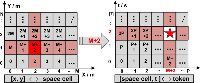
Space partition and token generation

References
Vlachos, M., Gunopulos, D., Kollios, G.: Discovering similar multidimensional trajectories. In: Agrawal, R., Dittrich, K.R. (eds.) Proceedings of the 18th International Conference on Data Engineering. https://doi.org/10.1109/ICDE.2002.994784. IEEE Computer Society (2002)
Chen, L., Özsu, M.T., Oria, V.: Robust and fast similarity search for moving object trajectories. In: Özcan, F. (ed.) Proceedings of the ACM SIGMOD International Conference on Management of Data. https://doi.org/10.1145/1066157.1066213, pp 491–502. ACM (2005)
Ranu, S., P, D., Telang, A.D., Deshpande, P., Raghavan, S.: Indexing and matching trajectories under inconsistent sampling rates. In: Gehrke, J., Lehner, W., Shim, K., Cha, S.K., Lohman, G.M. (eds.) 31st IEEE International Conference on Data Engineering, ICDE 2015. https://doi.org/10.1109/ICDE.2015.7113351, pp 999–1010. IEEE Computer Society (2015)
Chen, L., Ng, R.T.: On the marriage of lp-norms and edit distance. In: Nascimento, M.A., Özsu, M.T., Kossmann, D., Miller, R.J., Blakeley, J.A., Schiefer, K.B. (eds.) (e)Proceedings of the Thirtieth International Conference on Very Large Data Bases, VLDB 2004. https://doi.org/10.1016/B978-012088469-8.50070-X, http://www.vldb.org/conf/2004/RS21P2.PDF, pp 792–803. Morgan Kaufmann (2004)
Zheng, K., Zheng, Y., Xie, X., Zhou, X.: Reducing uncertainty of low-sampling-rate trajectories. In: IEEE 28th International Conference on Data Engineering (ICDE 2012). https://doi.org/10.1109/ICDE.2012.42, pp 1144–1155. IEEE Computer Society (2012)
Li, X., Zhao, K., Cong, G., Jensen, C.S., Wei, W.: Deep representation learning for trajectory similarity computation. In: 34th IEEE International Conference on Data Engineering, ICDE. https://doi.org/10.1109/ICDE.2018.00062, pp 617–628 (2018)
Pfoser, D., Jensen, C.S., Theodoridis, Y.: Novel approaches to the indexing of moving object trajectories. In: VLDB 2000, Proceedings of 26th International Conference on Very Large Data Bases. http://www.vldb.org/conf/2000/P395.pdf, pp 395–406. Morgan Kaufmann (2000)
Sun, S., Chen, J., Sun, J.: Traffic congestion prediction based on GPS trajectory data. Int. J. Distributed Sens Netw. 15(5). https://doi.org/10.1177/1550147719847440(2019)
Gomes, G.A.M., dos Santos, E.M., Vidal, C.A, da Silva, T.L.C., de Macêdo, J.A.F.: Real-time discovery of hot routes on trajectory data streams using interactive visualization based on GPU. Comput. Graph. 76, 129–141 (2018). https://doi.org/10.1016/j.cag.2018.09.008
Mikolov, T., Chen, K., Corrado, G., Dean, J.: Efficient estimation of word representations in vector space. In: ICLR (Workshop Poster) (2013)
Bütepage, J., Black, M.J., Kragic, D., Kjellström, H.: Deep representation learning for human motion prediction and classification. In: 2017 IEEE Conference on Computer Vision and Pattern Recognition, CVPR. https://doi.org/10.1109/CVPR.2017.173, pp 1591–1599 (2017)
Yao, H., Zhang, S., Hong, R., Zhang, Y., Xu, C., Tian, Q.: Deep representation learning with part loss for person re-identification. IEEE Trans. Image Process. 28(6), 2860–2871 (2019). https://doi.org/10.1109/TIP.2019.2891888
Rumhar, D., offry. Hnon‡, Wams, R.: Learning representations by back-propagating errors. Nature (1986)
Werbos, P.J.: Backpropagation through time: what it does and how to do it. Proc. IEEE 78(10), 1550–1560 (1990)
Zhang, Y., Dai, H., Xu, C., Feng, J., Wang, T., Bian, J., Wang, B., Liu, T.: Sequential click prediction for sponsored search with recurrent neural networks. In: Brodley, C. E., Stone, P (eds.) Proceedings of the Twenty-Eighth AAAI Conference on Artificial Intelligence. http://www.aaai.org/ocs/index.php/AAAI/AAAI14/paper/view/8529, pp 1369–1375. AAAI Press, Québec City (2014)
Gao, Q., Zhou, F., Zhang, K., Trajcevski, G., Luo, X., Zhang, F.: Identifying human mobility via trajectory embeddings. In: Sierra, C. (ed.) Proceedings of the Twenty-Sixth International Joint Conference on Artificial Intelligence, IJCAI. ijcai.org. https://doi.org/10.24963/ijcai.2017/234, pp 1689–1695 (2017)
Sutskever, I., Vinyals, O., Le, Q.V.: Sequence to sequence learning with neural networks. In: Advances in Neural Information Processing Systems 27: Annual Conference on Neural Information Processing Systems. http://papers.nips.cc/paper/5346-sequence-to-sequence-learning-with-neural-networks, pp 3104–3112 (2014)
Wang, H., Su, H., Zheng, K., Sadiq, S.W., Zhou, X.: An effectiveness study on trajectory similarity measures. In: ADC. CRPIT, vol. 137, pp 13–22 (2013)
Cancela, B., Ortega, M., Fernández, A., Penedo, M.G.: Trajectory similarity measures using minimal paths. In: Image Analysis and Processing - ICIAP 2013 - 17th International Conference, Naples, Italy, September 9-13, 2013. Proceedings, Part I. Lecture Notes in Computer Science. https://doi.org/10.1007/978-3-642-41181-6∖_41, vol. 8156, pp 400–409 (2013)
Frentzos, E., Gratsias, K., Theodoridis, Y.: Index-based most similar trajectory search. In: Chirkova, R., Dogac, A., Özsu, M.T., Sellis, T.K. (eds.) Proceedings of the 23rd International Conference on Data Engineering, ICDE 2007. https://doi.org/10.1109/ICDE.2007.367927, pp 816–825. IEEE Computer Society (2007)
Chen, L., Shang, S., Jensen, C.S., Yao, B., Zhang, Z., Shao, L.: Effective and efficient reuse of past travel behavior for route recommendation. In: Teredesai, A, Kumar, V., Li, Y., Rosales, R., Terzi, E., Karypis, G. (eds.) Proceedings of the 25th ACM SIGKDD International Conference on Knowledge Discovery & Data Mining, KDD. https://doi.org/10.1145/3292500.3330835, pp 488–498. ACM (2019)
Shang, S., Chen, L., Wei, Z., Jensen, C. S., Zheng, K., Kalnis, P.: Trajectory similarity join in spatial networks. Proc. VLDB Endow. 10(11), 1178–1189 (2017). https://doi.org/10.14778/3137628.3137630
Shang, S., Chen, L., Jensen, C.S., Wen, J., Kalnis, P.: Searching trajectories by regions of interest. IEEE Trans. Knowl. Data Eng. 29(7), 1549–1562 (2017). https://doi.org/10.1109/TKDE.2017.2685504
Shang, S., Ding, R., Zheng, K., Jensen, C.S., Kalnis, P., Zhou, X.: Personalized trajectory matching in spatial networks. VLDB J. 23 (3), 449–468 (2014). https://doi.org/10.1007/s00778-013-0331-0
Chen, L., Shang, S., Guo, T.: Real-time route search by locations. In: The Thirty-Fourth AAAI Conference on Artificial Intelligence, AAAI 2020, The Thirty-Second Innovative Applications of Artificial Intelligence Conference, IAAI 2020, The Tenth AAAI Symposium on Educational Advances in Artificial Intelligence, EAAI 2020. https://ojs.aaai.org/index.php/AAAI/article/view/5396, pp 574–581. AAAI Press (2020)
Zhang, C., Han, J., Shou, L., Lu, J., Porta, T.L.: Splitter: Mining fine-grained sequential patterns in semantic trajectories. Proc. VLDB Endow. 7(9), 769–780 (2014). https://doi.org/10.14778/2732939.2732949
Agrawal, R., Faloutsos, C., Swami, A.N.: Efficient similarity search in sequence databases. In: Lomet, D.B. (ed.) Foundations of Data Organization and Algorithms, 4th International Conference, FODO’93, Chicago, Illinois, USA, October 13-15, 1993, Proceedings. Lecture Notes in Computer Science. https://doi.org/10.1007/3-540-57301-1∖_5, vol. 730, pp 69–84 (1993)
Yi, B., Jagadish, H. V., Faloutsos, C.: Efficient retrieval of similar time sequences under time warping. In: Proceedings of the Fourteenth International Conference on Data Engineering. https://doi.org/10.1109/ICDE.1998.655778, pp 201–208. IEEE Computer Society (1998)
Cai, Y., Ng, R. T.: Indexing spatio-temporal trajectories with chebyshev polynomials. In: Weikum, G., König, A.C., Deßloch, S. (eds.) Proceedings of the ACM SIGMOD International Conference on Management of Data. https://doi.org/10.1145/1007568.1007636, pp 599–610. ACM (2004)
Shang, S., Ding, R., Yuan, B., Xie, K., Zheng, K., Kalnis, P.: User oriented trajectory search for trip recommendation. In: Rundensteiner, E.A., Markl, V., Manolescu, I., Amer-Yahia, S., Naumann, F., Ari, I. (eds.) 15th International Conference on Extending Database Technology. https://doi.org/10.1145/2247596.2247616, pp 156–167. ACM (2012)
Zheng, K., Shang, S., Yuan, N. J., Yang, Y.: Towards efficient search for activity trajectories. In: Jensen, C.S., Jermaine, C.M., Zhou, X. (eds.) 29th IEEE International Conference on Data Engineering. https://doi.org/10.1109/ICDE.2013.6544828, pp 230–241. IEEE Computer Society (2013)
Chen, L., Shang, S., Jensen, C. S., Yao, B., Kalnis, P.: Parallel semantic trajectory similarity join. In: 36th IEEE International Conference on Data Engineering, ICDE 2020. https://doi.org/10.1109/ICDE48307.2020.00091, pp 997–1008. IEEE (2020)
Shang, S., Chen, L., Wei, Z., Jensen, C.S., Zheng, K., Kalnis, P.: Parallel trajectory similarity joins in spatial networks. VLDB J. 27(3), 395–420 (2018). https://doi.org/10.1007/s00778-018-0502-0
Chen, L., Shang, S., Feng, S., Kalnis, P.: Parallel subtrajectory alignment over massive-scale trajectory data. In: Zhou, Z. (ed.) Proceedings of the Thirtieth International Joint Conference on Artificial Intelligence, IJCAI 2021, Virtual Event / Montreal, Canada, 19-27 August 2021. https://doi.org/10.24963/ijcai.2021/497, pp 3613–3619 (2021)
Shang, S., Chen, L., Zheng, K., Jensen, C.S., Wei, Z., Kalnis, P.: Parallel trajectory-to-location join. IEEE Trans. Knowl. Data Eng. 31(6), 1194–1207 (2019). https://doi.org/10.1109/TKDE.2018.2854705
Yao, D., Zhang, C., Zhu, Z., Huang, J., Bi, J.: Trajectory clustering via deep representation learning. In: 2017 International Joint Conference on Neural Networks, IJCNN. https://doi.org/10.1109/IJCNN.2017.7966345, pp 3880–3887. IEEE (2017)
Liu, Y., Zhao, K., Cong, G., Bao, Z.: Online anomalous trajectory detection with deep generative sequence modeling. In: 36th IEEE International Conference on Data Engineering, ICDE. https://doi.org/10.1109/ICDE48307.2020.00087, pp 949–960 (2020)
Zhang, Y., Liu, A., Liu, G., Li, Z., Li, Q.: Deep representation learning of activity trajectory similarity computation. In: 2019 IEEE International Conference on Web Services, ICWS. https://doi.org/10.1109/ICWS.2019.00059, pp 312–319 (2019)
Yao, D., Cong, G., Zhang, C., Bi, J.: Computing trajectory similarity in linear time: A generic seed-guided neural metric learning approach. In: 35th IEEE International Conference on Data Engineering, ICDE. https://doi.org/10.1109/ICDE.2019.00123, vol. 730, pp 1358–1369 (2019)
Zhang, H., Zhang, X., Jiang, Q., Zheng, B., Sun, Z., Sun, W., Wang, C.: Trajectory similarity learning with auxiliary supervision and optimal matching. In: Bessiere, C. (ed.) Proceedings of the Twenty-Ninth International Joint Conference on Artificial Intelligence, IJCAI 2020. https://doi.org/10.24963/ijcai.2020/444, pp 3209–3215 (2020)
Yang, C., Chen, L., Wang, H., Shang, S.: Towards efficient selection of activity trajectories based on diversity and coverage. In: Thirty-Fifth AAAI Conference on Artificial Intelligence, AAAI 2021, Thirty-Third Conference on Innovative Applications of Artificial Intelligence, IAAI 2021, The Eleventh Symposium on Educational Advances in Artificial Intelligence, EAAI 2021, Virtual Event, February 2-9, 2021. https://ojs.aaai.org/index.php/AAAI/article/view/16149, pp 689–696 (2021)
Zhao, Y., Chen, Q., Cao, W., Yang, J., Xiong, J., Gui, G.: Deep learning for risk detection and trajectory tracking at construction sites. IEEE Access 7, 30905–30912 (2019). https://doi.org/10.1109/ACCESS.2019.2902658
Fan, Z., Chen, Q., Jiang, R., Shibasaki, R., Song, X., Tsubouchi, K.: Deep multiple instance learning for human trajectory identification. In: Kashani, F.B., Trajcevski, G., Güting, R.H., Kulik, L., Newsam, S.D. (eds.) Proceedings of the 27th ACM SIGSPATIAL International Conference on Advances in Geographic Information Systems. https://doi.org/10.1145/3347146.3359342, pp 512–515 (2019)
Han, P., Wang, J., Yao, D., Shang, S., Zhang, X.: A graph-based approach for trajectory similarity computation in spatial networks. In: Zhu, F., Ooi, B.C., Miao, C. (eds.) KDD ’21: The 27th ACM SIGKDD Conference on Knowledge Discovery and Data Mining. https://doi.org/10.1145/3447548.3467337, pp 556–564. ACM (2021)
Bengio, Y., Courville, A.C., Vincent, P.: Representation learning: A review and new perspectives. IEEE Trans. Pattern Anal. Mach. Intell. 35(8), 1798–1828 (2013). https://doi.org/10.1109/TPAMI.2013.50
Miao, C., Wang, J., Yu, H., Zhang, W., Qi, Y.: Trajectory-user linking with attentive recurrent network. In: Seghrouchni, A.E.F., Sukthankar, G., An, B., Yorke-Smith, N. (eds.) Proceedings of the 19th International Conference on Autonomous Agents and Multiagent Systems, AAMAS. https://dl.acm.org/doi/abs/10.5555/3398761.3398864, pp 878–886. International Foundation for Autonomous Agents and Multiagent Systems (2020)
Wang, S., Bao, Z., Culpepper, J.S., Xie, Z., Liu, Q., Qin, X.: Torch: A search engine for trajectory data. In: Collins-Thompson, K., Mei, Q., Davison, B.D., Liu, Y., Yilmaz, E. (eds.) The 41st International ACM SIGIR Conference on Research & Development in Information Retrieval, SIGIR. https://doi.org/10.1145/3209978.3209989, pp 535–544. ACM (2018)
Xia, Y., Wang, G., Zhang, X., Kim, G. B., Bae, H.: Spatio-temporal similarity measure for network constrained trajectory data. Int. J. Comput. Intell. Syst. 4(5), 1070–1079 (2011). https://doi.org/10.1080/18756891.2011.9727855
Fu, T., Lee, W.: Trembr: Exploring road networks for trajectory representation learning. ACM Trans. Intell. Syst. Technol. 11(1), 10–11025 (2020). https://doi.org/10.1145/3361741
Yuan, H., Li, G.: Distributed in-memory trajectory similarity search and join on road network. In: 35th IEEE International Conference on Data Engineering, ICDE. https://doi.org/10.1109/ICDE.2019.00115, pp 1262–1273. IEEE (2019)
Newson, P., Krumm, J.: Hidden markov map matching through noise and sparseness. In: Agrawal, D., Aref, W.G., Lu, C., Mokbel, M.F., Scheuermann, P., Shahabi, C., Wolfson, O. (eds.) 17th ACM SIGSPATIAL International Symposium on Advances in Geographic Information Systems, ACM-GIS, 2009. https://doi.org/10.1145/1653771.1653818, pp 336–343. ACM (2009)
Lou, Y., Zhang, C., Zheng, Y., Xie, X., Wang, W., Huang, Y.: Map-matching for low-sampling-rate GPS trajectories. In: Agrawal, D., Aref, W.G., Lu, C., Mokbel, M.F., Scheuermann, P., Shahabi, C., Wolfson, O. (eds.) 17th ACM SIGSPATIAL International Symposium on Advances in Geographic Information Systems, ACM-GIS. https://doi.org/10.1145/1653771.1653820, pp 352–361. ACM (2009)
Brakatsoulas, S., Pfoser, D., Salas, R., Wenk, C.: On map-matching vehicle tracking data. In: Böhm, K., Jensen, C.S., Haas, L.M., Kersten, M.L., Larson, P., Ooi, B.C. (eds.) Proceedings of the 31st International Conference on Very Large Data Bases. http://www.vldb.org/archives/website/2005/program/paper/fri/p853-brakatsoulas.pdf, pp 853–864. ACM (2005)
Yuan, J., Zheng, Y., Zhang, C., Xie, X., Sun, G.: An interactive-voting based map matching algorithm. In: Hara, T., Jensen, C.S., Kumar, V., Madria, S., Zeinalipour-Yazti, D. (eds.) Eleventh International Conference on Mobile Data Management, MDM. https://doi.org/10.1109/MDM.2010.14, pp 43–52. IEEE Computer Society (2010)
Su, H., Zheng, K., Wang, H., Huang, J., Zhou, X.: Calibrating trajectory data for similarity-based analysis. In: Proceedings of the ACM SIGMOD International Conference on Management of Data, SIGMOD. https://doi.org/10.1145/2463676.2465303, pp 833–844 (2013)
Güting, R.H., Schneider, M.: Realm-based spatial data types: The ROSE algebra. VLDB J. 4(2), 243–286 (1995)
Schroff, F., Kalenichenko, D., Philbin, J.: Facenet: A unified embedding for face recognition and clustering. In: CVPR, pp 815–823 (2015)
Yuan, J., Zheng, Y., Xie, X., Sun, G.: Driving with knowledge from the physical world. In: Proceedings of the 17th ACM SIGKDD International Conference on Knowledge Discovery and Data Mining. https://doi.org/10.1145/2020408.2020462, pp 316–324 (2011)
Yuan, J., Zheng, Y., Zhang, C., Xie, W., Xie, X., Sun, G., Huang, Y.: T-drive: driving directions based on taxi trajectories. In: 18th ACM SIGSPATIAL International Symposium on Advances in Geographic Information Systems, ACM-GIS 2010. https://doi.org/10.1145/1869790.1869807, pp 99–108 (2010)
Su, H., Liu, S., Zheng, B., Zhou, X., Zheng, K.: A survey of trajectory distance measures and performance evaluation. VLDB J. 29(1), 3–32 (2020). https://doi.org/10.1007/s00778-019-00574-9
Acknowledgements
We also acknowledge the editorial committee’s support and all anonymous reviewers for their insightful comments and suggestions, which improved the content and presentation of this manuscript.
Funding
This work was supported by the NSFC (U2001212, U21B2046, 62032001, and 61932004).
Author information
Authors and Affiliations
Contributions
All authors contributed to the study conception and model design. Ziwen Chen and Ke Li worked on the full manuscript. The first draft of the manuscript was written by Ziwen Chen and Ke Li. Lisi Chen and Shuo Shang wrote the Section 1–2. Ziwen Chen and Ke Li prepared the Section 3–5. The expermental study was conducted by Silin Zhou. All authors commented on previous versions of the manuscript. All authors proof-read and approved the final manuscript.
Corresponding author
Ethics declarations
Competing interests
We declare that authors have no known competing interests or personal relationships that might be perceived to determine the discussion report in this paper.
Additional information
Publisher’s note
Springer Nature remains neutral with regard to jurisdictional claims in published maps and institutional affiliations.
Ke Li is the contact author.
Rights and permissions
About this article

Cite this article
Chen, Z., Li, K., Zhou, S. et al. Towards robust trajectory similarity computation: Representation-based spatio-temporal similarity quantification. World Wide Web 26, 1271–1294 (2023). https://doi.org/10.1007/s11280-022-01085-4
Received:
Revised:
Accepted:
Published:
Issue Date:
DOI: https://doi.org/10.1007/s11280-022-01085-4