
Abstract
This paper concerns a disassembly line balancing problem (DLBP) in remanufacturing that aims to allocate a set of tasks to workstations to disassemble a product. We consider two objectives in the same time, i.e., minimising the number of workstations required and minimising the operating costs. A common approach to such problems is to covert the multiple objectives into a single one and solve the resulting problem with either exact or heuristic methods. However, the appropriate weights must be determined a priori, yet the results provide little insight on the trade-off between competing objectives. Moreover, DLBP problems are proven NP-complete and thus the solvable instances by exact methods are limited. To this end, we formulate the problem into a multi-objective dynamic program and prove the monotonicity property of both objective functions. A backward recursive algorithm is developed to efficiently generate all the non-dominated solutions. The numerical results show that our proposal is more efficient than alternative exact algorithms proposed in the literature and can handle much larger problem instances.
1 Introduction
For environmentally conscious and sustainable manufacturing, a growing number of manufacturers have started to recycle and remanufacture their end-of-life (EOL) products after these products are discarded by consumers. Product recovery can minimise the amount of waste sent to landfills and exploit economic gains through recycling and remanufacturing. The first essential step in product recovery is disassembly, which is defined as the methodological extraction of valuable parts/subassemblies and materials from discarded products via a series of operations (McGovern and Gupta 2010). Efficient retrieval of these parts/subassemblies cuts down the production cost, reduces the associated disposal cost and, consequently, the environmental hazards.
Disassembly operations can be processed at a single workstation, in a disassembly cell or through a disassembly line. Compared with the other two settings, disassembly lines achieve the highest productivity rate; they are also the most appropriate design for either large products or small products in large quantities. A disassembly line includes a number of ordered workstations that sequentially disassemble products into individual components. The lines may take different shapes such as straight, U-shaped, parallel and two-sided. The most studied layout is the straight disassembly line in the literature. A major challenge for disassembly lines is the so called Disassembly Line Balancing Problem (DLBP), which concerns the allocation of disassembly tasks to successive workstations so as to build a feasible sequence that satisfies system constraints (such as precedence relations, assignment restrictions and cycle time constraints), and in the mean time optimises a pre-defined performance measure. Various measures have been considered in the literature, including the number of workstations (Koc et al. 2009; Mete et al. 2016; Altekin 2016, 2017; Li et al. 2019, 2019a), the level of balance between workstations’ idle times (Duta et al. 2005; Riggs et al. 2015; Kannan et al. 2017), and the profit or revenue (Kalaycilar et al. 2016; Ren et al. 2017). All these works focus on single objective optimization problems. Since DLBP problems are NP-Complete (McGovern and Gupta 2007), both the exact and heuristic solution approaches have been proposed in the literature. Although heuristic methods have their advantage in finding good solutions within reasonable time frame, the results obtained heavily rely on the heuristic rules and are not guaranteed to be optimal. In contrast, the exact methods can obtain optimal solutions for small-scale problems, whereas they are not suitable for larger scale problems due to the prohibitive computational effort required.
In the last few years many researchers have been arguing that multiple objectives should be considered in practical DLBP problems. Indeed, it is often desirable to achieve trade-offs among several competing objectives such as the minimum number of disassembly workstations used, the optimal assignment of tasks to each workstation, the maximum profit or minimum cost, and etc. To address multiple objective DLBP (MODLBP), a common treatment is to convert multiple objectives into a single one by the assignment of weights to each goal (Tuncel et al. 2012). However, as we all understand, it is difficult for decision-makers to represent their preferences on each goal using physically meaningful preference ranges. Setting the weight values reasonably and accurately is therefore a major hurdle for such approaches. Alternatively, the pre-emptive lexicographic perspective (Kalayci et al. 2016) method focuses on the optimization of the objectives once a time, which fails to achieve the balance among multiple objectives and losses the diversity of solutions. Both types of methods cannot ensure that the obtained solutions are really what expected, as they yield limited insight on the trade-off between different objectives and provide few options to the decision maker. Moreover, most of the previous works in the literature focus on heuristics or meta-heuristic methods to obtain near-optimal solutions. Recent examples include genetic algorithms (Aydemir-Karadag and Turkbey 2013), ant colony optimisation (Ding et al. 2010), and firefly optimization (Zhu et al. 2018).
As far as we know there are no exact methods proposed in the literature to solve MODLBP problems directly. Thus, this research makes the first attempt to solve the MODLBP with an efficient dynamic programming (DP) approach, which is capable of generating all the non-dominated solutions within reasonable time, even for some large size instances. To the best of our knowledge, the application of DP approaches to DLBP problems is rare. The only precursor to our paper is due to Koc et al. (2009), who considered a single objective DLBP problem and developed a DP approach to solve it. Their numerical results show that the DP approach performs stronger than an integer programming (IP) approach in terms of the solvable sizes of the problem. Unlike Koc et al. (2009) we consider a more realistic DLBP problem with two objectives. Moreover, the DP approach proposed in Koc et al. (2009) suffers the dimensionality issue of dynamic programming. They struggled to solve problems with moderate sizes. This is due to the partial AND/OR Graphs (AOG) that are used to represent the states in their DP formulation. Such a treatment leads to rapid increase of the state space with the product complexity/size and the number of alternative tasks. In fact, to just find all the partial AOGs for all subassemblies is not a trivial task. Moreover, all these partial AOGs need to be found and stored before the forward recursion is undertaken to calculate the value functions, which consumes a large amount of memory. To this end, we exploit the structure of the problem concerned and propose a different DP formulation with backward recursion. The states are simply defined as subassemblies rather than their associated partial AOG graphs. The numerical experiments show that our proposed approach is much more efficient than alternative exact algorithms proposed in the literature, and capable of solving much larger problem instances.
The remainder of the paper is organized as follows. Section 2 reviews the relevant literature on DLBP problems and Sect. 3 describes in detail the problem concerned. The proposed DP method is explained in Sect. 4. Its performance is tested extensively on realistic cases and benchmark problems in Sect. 5. Section 6 concludes the paper.
2 Literature review
The single objective DLBP problems have been well studied in the literature. Both heuristics and exact approaches have been developed to solve such problems. Gungor and Gupta (2001) proposed a solution approach to the DLBP in the presence of task failures. The approach involves the following steps: (1) generate an incomplete state network representing all feasible states and their partial relationships; (2) generate the weights of edges based on the idle times of task assignments; (3) apply the Dijkstra’s shortest path algorithm to generate all shortest directed paths between the source node and the final node of the weighted state network. Recently, Altekin (2017) presented two second-order cone programming models and five piecewise linear mixed integer programming models for the DLBP with stochastic task times. The task times are assumed to be normally distributed with known means and variances. Their objective is to minimise the number of workstations needed. All these seven models are shown to be able to solve practical-sized problems. Li et al. (2019) developed a branch-bound-remember (BBR) algorithm for a simple DLBP with an objective to minimise the number of stations for parallel tasks. They also proposed two lower bounding schemes, a strengthened Koc’s IP model (Koc et al. 2009) and a new benchmark instance generation scheme. Computational results show that this branch-bound-remember algorithm solves most of the instances considered in short time. The lower bounds and the strengthened IP model are also demonstrated to be effective. Riggs et al. (2015) showed that generating a (stochastic) joint precedence graph based on the different EOL states of a product is beneficial to achieve the optimal line balance that considers both deterministic and stochastic task times. To deal with multiple types of products, Kannan et al. (2017) proposed a cost effective reverse logistics network from the perspective of the third party to work with a balanced disassembly line. A mixed integer non-linear program is developed and validated using various products from the liquid crystal displays industry.
There have been some attempts to optimally solve profit-oriented DLBP. Altekin et al. (2008) defined and solved a profit-oriented partial DLBP problem. They developed the first mixed integer programming formulation, and proposed a lower and upper-bounding scheme based on linear programming relaxation. Their computational results show that the approach provides near optimal solutions for small problems and is capable of solving larger problems with up to 320 disassembly tasks in reasonable time. Ren et al. (2017) considered a similar problem and established a mathematical model to achieve the maximisation of profit, which is solved by an improved gravitational search algorithm (GSA). Kalaycilar et al. (2016) considered a DLBP with a fixed number of workstations and presented several upper and lower bounding procedures to maximise the total net revenue. Refer to Deniz and Ozcelik (2019) for a recent and comprehensive review on DLBP problems.
MODLBP have received increasing attention over the last decade. McGovern and Gupta (2007) considered an MODLBP problem that aims to minimise the number of workstations, balance the workstation idle time, remove hazardous parts early in the disassembly sequence, remove high-demand parts before low demand parts and minimise the number of part removal direction changes required for disassembly. They proposed a recursive exhaustive search algorithm to find optimal solutions for small sized problem instances and a genetic algorithm to find high quality solutions for large sized instances. Zhang et al. (2017) investigated an MODLBP with fuzzy disassembly times, in which tasks’ disassembly times were assumed as triangular fuzzy numbers. A Pareto improved artificial fish swarm algorithm (IAFSA) was proposed to solve the problem. They tested their algorithm with four objectives: number of workstations, workload balance between workstations, disassembly cost and disassembly direction change frequencies. An MODLBP mathematical model was presented by Zhu et al. (2018) for minimising the number of workstations, maximising the smoothing rate and minimising the average maximum hazard of the disassembly line. A Pareto firefly algorithm (FA) was proposed to solve the problem. Compared with other algorithms, the proposed Pareto firefly algorithm finds more Pareto optimal solutions. Fang et al. (2019) focused on evolutionary many-objective optimisation for mixed-model DLBP with multi-robotic workstations. A mathematical program was proposed to minimise the cycle time, the total energy consumption, the peak workstation energy consumption, and the number of robots being used simultaneously.
It is worth mentioning that some important variants of the DLBP problems have been studied. Sequence-dependent disassembly line balancing problem (SDDLBP) is an extension to the DLBP. SDDLBP augments sequence-dependent time considerations to DLBP. SDDLBP with multiple objectives was first introduced in Kalayci and Gupta (2013a) and solved by meta-heuristic techniques such as ant colony optimization (ACO) (Kalayci and Gupta 2013a), particle swarm optimisation (PSO) (Kalayci and Gupta 2013b), (improved) artificial bee colony (ABC) (Kalayci and Gupta 2013c), (improved) discrete artificial bee colony (DABC) (Liu and Wang 2017), simulated annealing (SA) (Kalayci and Gupta 2013d), river formation dynamic approach (RDF) (Kalayci and Gupta 2013e), tabu search (TS) (Kalayci and Gupta 2014), variable neighbourhood search (VNS) (Kalayci et al. 2015) and hybrid GA (VNSGA) algorithm (Kalayci et al. 2016). Parallel DLBP (PDLBP) was first introduced by Hezer and Kara (2015), who considered two or more straight disassembly lines which are balanced simultaneously. Hezer and Kara (2015) proposed a network model based on the shortest route model (SRM) for PDLBP to minimise the number of workstations. The procedure of SRM consists node generation, arc construction, and shortest route identification to construct the network model.
To summarise, we list the relevant works in the recent literature in Table 1, with respect to the number of objectives, the line type, the precedence relation representation, and the solution approaches. It clearly shows the lack of exact methods to solve MODLBP problems.
3 Problem description
This paper considers a single type of product that undergoes a number of ordered tasks for complete disassembly. Each task leads to the removal of one part except the final task that results in the separation of two parts. There may exist several different disassembly sequences or routes. We follow Koc et al. (2009) and use Transformed AND/OR Graphs (TAOG) to depict all the possible alternative sequences for disassembly. A TAOG is a modified version of an AOG with explicit information on the precedence relationship between tasks. Both the TAOG and task precedence diagram (TPD) include information about the task precedence relations that should be considered in the assembly/disassembly process. A task in the TAOG is defined based on the current subassembly and the part to be removed immediately, whereas that in the TPD is defined only in terms of the removed part. This leads to different labelling of tasks between TAOG and TPD.
We use a sample product to illustrate the relationship between the disassembly sequences and TAOG/TPD. As shown in Fig. 1a, the sample product consists of five parts, which can be fully disassembled via different sequences as shown in the AOG (Fig. 1b). The nodes in the AOG represent subassemblies while the arcs the corresponding disassembly tasks. A subassembly contains at least two parts. The root node represents the original product yet to be disassembled. The derived TAOG is shown in Fig. 1c, where the artificial nodes (A) represent subassemblies and the normal nodes (B) represent disassembly tasks in the AOG. Two types of arcs exist in TAOG. The regular one-to-one precedence relation is represented by the AND-type, while the multiple and alternative precedence relations are represented by the OR-type (indicated with a small curve in Fig. 1c). In the latter situation a subassembly could be disassembled via alternative tasks. The correspondence between subassemblies and artificial nodes in the TAOG is listed in Table 2.

A sample product and its TAOG and TPDs
The original product (1-5) is represented by \(A_0\). Note that we have inserted a final artificial node \(A _{12}\) to represent that the disassembly is completed. The disassembly procedure starts with a task of either \(B_1, B_2\) or \(B_3\) and ends with a task of either \(B_{19}, B_{20},B_{21}\) or \(B_{22}\). For example, all alternative feasible routes which start with \(B_3\) are listed as follows:
-
(1)
A\(_0\)-B\(_3\)-A\(_3\)-B\(_9\)-A\(_6\)-B\(_{15}\)-A\(_9\)-B\(_{20}\)-A\(_{12},\)
-
(2)
A\(_0\)-B\(_3\)-A\(_3\)-B\(_9\)-A\(_6\)-B\(_{16}\)-A\(_{10}\)-B\(_{21}\)-A\(_{12},\)
-
(3)
A\(_0\)-B\(_3\)-A\(_3\)-B\(_{10}\)-A\(_7\)-B\(_{17}\)-A\(_{10}\)-B\(_{21}\)-A\(_{12},\)
-
(4)
A\(_0\)-B\(_3\)-A\(_3\)-B\(_{10}\)-A\(_7\)-B\(_{18}\)-A\(_{11}\)-B\(_{22}\)-A\(_{12}.\)
For each feasible route, the product is disassembled completely.
The derived TPDs are shown in Fig. 1d, even though they are not used in this work. Firstly we define equitasks as the tasks that remove the same part. For example, tasks 1, 7, 9 and 17 are equitasks as they all lead to the removal of part 1; they are denoted by the same letter a in TPDs. The equitasks for other parts are denoted in the same manner, except the final tasks which are denoted by their original numbers. The mapping between TAOG and TPD tasks are shown in Table 3.
From each TPD multiple and alternative feasible sequences can be derived. For example one can obtain from TPD\(_1\) three alternative feasible sequences (b-a-d-19, a-b-d-19, a-d-b-19). For more details on TPDs refer to Koc et al. (2009).
A number of workstations are located along the disassembly line to complete the tasks. Even though they are capable of processing all these tasks, each workstation is only allowed to work for a limit amount of time due to the cycle time constraint. In other words, the sum of disassembly time of all the tasks assigned to a workstation must be within the pre-defined cycle time (CT). Moreover, each task can be assigned to one and only one workstation, and the precedence relationship among the tasks must not be violated.
Our aim is to find feasible allocation of tasks to workstations which meets these constraints and in the mean time achieves pre-defined objectives. We consider two objectives in this paper, as explained below.
-
Objective 1: Minimum number of workstations required. The first objective concerns the total number of workstations required to disassemble the product. Reducing the number of workstations means shorter production lines and less employees required, both of which enhance the resource utilisation. Fewer workstations are always preferred.
-
Objective 2: Minimum total disassembly task cost. The second concerns the operating cost to perform the assigned disassembly tasks, which are typically manual and labour intensive. The disassembly task costs are dependent upon the disassembly tools and operating orders. Therefore, the costs incurred could be quite different between disassembly sequences.
These two objectives are often conflicting, as demonstrated in the example in Fig. 2, where B\(_1\)-B\(_3\)-B\(_5\)-B\(_7\)-B\(_9\) and B\(_2\)-B\(_4\)-B\(_6\)-B\(_8\)-B\(_{10}\) are two feasible and complete disassembly sequences for a product. The first disassembly sequence requires 4 workstations with a total disassembly cost 57, whereas the second requires only 3 workstations but a total disassembly task cost of 65. To address this multiple objective decision making problem, we propose in this paper an efficient dynamic programming approach to find all the non-dominated disassembly sequences. A disassembly sequence is said to be dominated by another if its performance is weaker than the latter on both objectives.
Before we introduce the dynamic programming solution approach in the next section, it is worth mentioning that we restrict our attention to sequential tasks in this work, as shown in Fig. 1c. In other words, there is at most one outbound arc from any task node. The problems with parallel tasks are much more complicated, even with just a single objective (Koc et al. 2009); we will address them (with multiple objectives) in another work.
4 A DP approach for the DLBP
The problem alluded to in the previous section can be modelled as a dynamic program, as illustrated below.
-
Stage \(k=1,2,\ldots ,N\).
-
State is defined as the subassemblies at each stage k. It is obvious that when \(k=1\) the single state is the original product containing all parts. When \(k=2\), one part should have been disassembled and the state is a subassembly containing the remaining parts, and so on. At stage N-1 the state is a combination of just two parts which are readily disassembled. Mathematically, we define state at stage k as a vector \(x_k=(i_1, i_2,\ldots ,i_m,\ldots ,i_{N-k+1})\), where \(i_m\) is the part index. Note that the dimension of \(x_k\) is always \(N-k+1\), since only one part is disassembled each stage. A state is essentially one artificial node in TAOG as shown in Fig. 1b. No two states are the same between stages. We denote the state for the final stage by an empty state \(x_N=\emptyset \).
-
We define actions as the admissible disassembly tasks for a state. Denote the set of all admissible tasks as \({\mathcal {U}}(x_k)\) for state \(x_k\). For example, for state \(A_1\) at stage 2 in Fig. 1c, the admissible set of tasks is \({\mathcal {U}}(A_1)=\{B_4, B_5, B_6\}\). Each action \(u_k \in {\mathcal {U}}(x_k)\) takes \(t_{u_k}\) time to finish and incur a cost of \(c_{u_k}\). After taking the action \(u_k \in {\mathcal {U}}(x_k)\) in state \(x_k\) the system transits into state \(x_{k+1}\) at the next stage.
-
A policy \(\pi = (u_1,u_2,\cdots ,u_N)\) is a sequence of actions that completely disassemble the product. Similarly, we define a partial policy \((u_k,u_{k+1},\cdots ,u_N)\) for the tail subproblem that starts from state \(x_k\) at stage k. For each state \(x_k\), denote the set of all feasible partial policies by \(\varPi (x_k)\). Therefore \(\varPi (x_1)\) represents the set of feasible disassembly polices for the product. For simplicity we use \(\pi \) to denote both partial and full policies. Each policy \(\pi \) describes a one to one mapping from states to actions, denoted as \(u_k = \pi (x_k)\).
-
Cost functions. Let \({\varvec{C}}^{\pi }_k(x_k) =(C_k^{\pi ,1}(x_k), C_k^{\pi ,2}(x_k))\) be a vector of the total value for each objective when starting from state \(x_k\) and following policy \(\pi \in \varPi (x_k)\). For each objective \(p \in \{1,2\}\), the cost is calculated via the recursive equation below.
$$\begin{aligned} C^{\pi ,p}_k(x_k)= {\left\{ \begin{array}{ll} C^{\pi ,p}_{k+1}(f(x_k,u_k)))+ g^{\pi ,p}(x_k), &{} \text{ if } k \le N-1, \\ 0, &{} \text{ otherwise }. \end{array}\right. } \end{aligned}$$Fig. 2 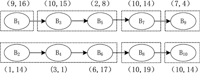
Two feasible disassembly sequence with tasks featured by (t, c), where t is the task time and c is the cost. Cycle time is 15
A list of notation used to describe the DLBP problem is described below.
Table 4 List of notation where \(f(x_k,u_k)\) is the state transition function under policy \(\pi \), and \(g^{\pi ,p}(x_k)\) the immediate cost calculated as follows.
$$\begin{aligned} g^{\pi ,1}(x_k)&=\varGamma (C_{k+1}^{\pi ,1}(f(x_k,u_k)),t_{u_k}),\\ g^{\pi ,2}(x_k)&= c_{u_k}, \end{aligned}$$where
$$\begin{aligned}\varGamma (x ,y )= {\left\{ \begin{array}{ll} \lfloor x+y/CT \rfloor -x+y/CT, &{}\text{ if } \lfloor x \rfloor<\lfloor x+y/CT\rfloor <x+y/CT,\\ y/CT, &{}\text{ if } \lfloor x+y/CT\rfloor =\lfloor x \rfloor or \lfloor x+y/CT\rfloor =x+y/CT. \end{array}\right. }\end{aligned}$$The above equation can be interpreted as follows; if the idle time in the last workstation under the partial policy \(\pi \in \varPi (x_k)\) is greater than or equal to \(t_{u_k}\), then \(\varGamma =t_{u_k}/CT\); otherwise, a new workstation is opened. Hence, the unused idle time is added to \(t_{u_k}/CT\) in the computation of \(\varGamma \). \(\lfloor x \rfloor \) rounds down x to the nearest integer. Further, for each objective p, define by \({\mathcal {Z}}^p(x_k)=\{C^{\pi ,p}_k(x_k) |\pi \in \varPi (x_k)\} \) the set containing the cost under all partial policies for the tail subproblem.
-
A cost vector \({\varvec{C}}_k(x_k)\) is said to dominate \({\varvec{C}}'_k(x_k)\) if \(C^p_k(x_k)\le C'^p_k(x_k)\) for all p, with strict inequality held for at least one p. Let \(\varvec{{\mathcal {F}}}_k(x_k)\) be the set of all non-dominated cost vectors for state \(x_k\).

Our objective is to find all the non-dominated cost vector sets \(\varvec{{\mathcal {F}}}_k(x_k), k = 1,2,\ldots ,N-1\), along with the corresponding optimal, non-dominated policies. To this end, we first show that the cost functions for both objectives satisfy the monotonicity property (Montoya et al. 2014; Carraway et al. 1990).
Proposition 1
(Monotonicity property) For each objective p, the cost function holds the monotonicity property. Specifically,
-
i)
for any \(z_1, z_2 \in {\mathcal {Z}}^1(x_k), \pi \in \varPi (x_k), 0<t\le CT\), if \(z_1 \le z_2\), we have \(z_1 + g^{\pi ,1}(x_k) \le z_2 + g^{\pi ,1}(x_k)\) (i.e., \(z_1 + \varGamma (z_1, t) \le z_2 + \varGamma (z_2, t)\));
-
ii)
for any \(z_1, z_2 \in {\mathcal {Z}}^2(x_k), \pi \in \varPi (x_k)\), if \(z_1 \le z_2\), we have \(z_1 + g^{\pi ,2}(x_k) \le z_2 + g^{\pi ,2}(x_k)\).
Proof
(i) for any \(z_1, z_2 \in {\mathcal {Z}}^1(x_k)\), \(\varGamma (z_1, t)\) and \(\varGamma (z_1, t)\) could take the following values.
Situations (a) and (c) mean that a new workstation is to be opened if a task of time t is assigned; while (b) and (d) mean that there is no need to open a new workstation. There are four combination cases of these situations.
Case 1 (a and c): if \(z_1 \le z_2\), we have \(\lfloor z_1+t/CT \rfloor \le \lfloor z_2+t/CT \rfloor \), and thus
Case 2 (a and d): this case is only possible when \(z_1<z_2\). We first show that \(\lfloor z_1 \rfloor \ne \lfloor z_2 \rfloor \). To see this, if \(\lfloor z_1 \rfloor = \lfloor z_2 \rfloor \) we have from situation (a)
which contradicts with the first condition in (d). Moreover, due to \(t/CT \le 1\) we have
Rearranging the equation we have
and thus \(z_2 +t/CT>1+\lfloor z_2 \rfloor \ge \lfloor z_2+t/CT \rfloor \), which contradicts with the second condition in (d).
Therefore \(\lfloor z_1 \rfloor < \lfloor z_2 \rfloor \), which means that the integer part of \(z_2\) is at least 1 more than that of \(z_1\). We then have \(\lfloor z_1+t/CT \rfloor \le \lfloor z_2 \rfloor < z_2\), and
Case 3 (b and c): this case is only possible when \(z_1<z_2\). From situation (c) and \(t/CT \le 1\), we have \(\lfloor z_2+t/CT \rfloor = \lfloor z_2 \rfloor +1 > z_2\), and thus
Case 4 (b and d): the conclusion is obvious.
(ii) the proof is trivial for the additive linear cost function. \(\square \)
The above property ensures the validity of the Principal of Pareto-Optimality (Daellenbach and De Kluyver 1980) of the multi-objective DP problem concerned. It allows us to calculate all the non-dominated cost vector sets \(\varvec{{\mathcal {F}}}_k(x_k)\) recursively as follows. Given the set \(\varvec{{\mathcal {F}}}_{k+1}(x_{k+1})\) for all states \(x_{k+1}\), the proposed algorithm first generates for each state \(x_k\) the set of cost vectors
such that \((C^1, C^2)\in \varvec{{\mathcal {F}}}_{k+1}(f(x_k,u_k)), \forall u_k \in {\mathcal {U}}(x_k)\). Then \(\varvec{{\mathcal {F}}}_k(x_k)\) is obtained by discarding from this set the vectors that are dominated by the other vectors. The boundary condition is that \(\varvec{{\mathcal {F}}}_N(\emptyset )\) just contains a zero vector. The recursive procedure is described as follows to compute \(\varvec{{\mathcal {F}}}_k(x_k)\) and the corresponding disassembly tasks.

Remark 1
In Algorithm 1 we have calculated the cost function for both objectives via backward recursion. In other words, the algorithm starts from stage N and updates the cost functions backwards, while the actual disassembly process is undertaken forwards. However, it can be readily proved that for any feasible disassembly sequence, the resulting final cost function values for both objectives are essentially the same. The result is trivial for the second objective. For the first one it can be proved by contradiction. For brevity we do not provide this rather straightforward proof.
5 Computational experiments
We first demonstrate the solution process of the proposed DP algorithm and its result via an illustrated example in Sect. 5.1. In Sect. 5.2 its performance is evaluated over a number of problem instances. Since our work is the first exact approach to solve multiple objective DLBP problems, there are not any comparable exact algorithms in the literature. Even though some heuristics have been developed for such problems, they are not comparable either. Instead, we have decided to evaluate the DP algorithm against another exact solution approach (SRM) that is designed for single objective DLBP problems, as follows. For each problem instance, we applied the DP algorithm and found all the non-dominated cost vectors, which also include the optimal values for each objective. Then we applied the SRM algorithm twice to the same problem; each time a different objective was considered. Since both are exact algorithms, their solutions (on each objective) would always be the same. Therefore we compared the solution time and the amount of solvable cases. The algorithms were implemented in MATLAB and tested on a personal computer with an Intel(R) Core(TM) processor of 2.70GHz clock speed and 8 GB RAM.
5.1 An illustrative example
We have introduced the example problem in Sect. 3. Figure 1c shows the TAOG of the sample product; it contains 22 normal nodes and 12 artificial nodes. The complete set of data of the example is listed in Table 5. The cycle time was set to 16 min.
Table 6 summarises the computational results for this example. For each stage, the non-dominated cost vectors for each state are listed, next to the corresponding disassembly tasks. For example, for state \(A_4\) at stage 3 there are two non-dominated vectors (0.625, 7) and (1, 5), with the corresponding actions \(B_{11}\) and \(B_{12}\), respectively. The results show that the optimal value is 1.125 for the first objective and 14 for the second, which are included in the four non-dominated cost vectors at stage 1. We now demonstrate how to derive the policies implied in these results. For instance to find the policy that minimises objective 1, we start with state \(A_0\) at stage 1 and identify the cost vector with the minimum value in this objective, which is (1.125, 18). The corresponding action \(B_3\) is then the first task in the policy, which leads to state \(A_3\) in the next stage (Fig. 1c). Given \(t_{B_3}=2,c_{B_3}=5\) we know that the action to take at \(A_3\) is \(B_9\), leading to the the next state \(A_6\). The same procedure is repeated until the last stage, and we find the optimal sequence for the first objective is B\(_3\)-B\(_9\)-B\(_{16}\)-B\(_{21}\). Similarly for objective 2, the optimal sequence is B\(_3\)-B\(_{10}\)-B\(_{18}\)-B\(_{22}\).
5.2 Performance evaluation
In this section the performance of the proposed DP approach was tested and compared against the SRM approach by Hezer and Kara (2015) over a number of problem instances. We followed the scheme proposed by Koc et al. (2009) to generate the instances according to three parameters (a, q, N), where a is the number of states (i.e. artificial nodes) at each stage and q the number of admissible tasks (normal nodes) for each state (except those at stage 1 and \(N-1\)), as demonstrated in the example in Fig. 3. The total number of artificial nodes is given by \(a\times (N-2)+2\), and the total number of normal nodes \(a\times (t\times (N-3)+2)\). The details on how these test problems are generated can be found in Koc et al. (2009).

An example of the TAOG \((a,q,N)=(3,2,5)\)
Three different cycle times \((CT=10, 15, 20)\) were considered. The instances with \(a=2,3\), \(q=1,2\), and \(N=5\sim 10\) were considered as small size problems. The task time of the normal nodes were generated randomly from a discrete uniform distribution U[2, 8] (Mete et al. 2016). The disassembly cost of each task was generated randomly from a discrete uniform distribution U[1, 20]. In total 69 small problems were generated, each of which was solved by both DP and SRM. The optimal values of each objective and the CPU time (seconds) for both algorithms are given in Table 7. The first column indicates the test problem parameters and the second cycle time. The next three columns show the optimal solutions of each objective and the CPU time for DP, while the last four the optimal solutions and the CPU time for each run of SRM.
As shown in Table 7, the number of workstations required \(\left\lceil f_1 \right\rceil \) and the total operating cost \(f_2\) obtained by both algorithms are always the same over all problem instances, as expected. They are both very efficient with less than 0.1 second CPU time for these small instances. The DP algorithm, however, only ran once to obtain the optimal solutions for both objectives individually, along with all the non-dominated policies that are not available in the SRM solution.
We continued the experiment for medium size problems with \(a=2\sim 10; q=3\sim 10; N=15\). The task times and costs were generated from the discrete uniform distribution U[1, 20]. The cycle time was set at both 1.5 and 2 times of the longest task time (Mete et al. 2016). In total 34 test cases were generated and the results are given in Table 8. Note that OT/OM stands for over time/out of memory; in either situation no solutions were obtained. According to Table 8, the DP approach found the optimal solutions for all problems with less CPU time than SRM. For fixed N, a larger value of q (or a) increases the CPU time remarkably. Moreover, the more the number of normal tasks and parts, the stronger the DP’s performance compared to SRM. In addition, for fixed a and N, an increase in q results in a larger solution space, and thus consumes more CPU time or even leads to out of memory for SRM. This is because SRM checks all possibility to guarantee the optimal solution. This is however not the case for DP that eliminates a large proportion of partial sequences that are dominated at each stage.
Finally a number of large problem instances were studied, with \(a=3,4,5,10, q=2, 3, 5, 10\) and \(N=20, 50, 80\). In total we have generated 96 instances and the results are summarised in Table 9. SRM is no more applicable to such large problems and thus only the solution time of DP is reported. It is shown that the DP approach was still strong and found the optimal solutions for all problems within a short time. Even for the very large instances with \(a=10,q=10, N=80\) the solution time is just 22.8 seconds, while in sharp contrast the DP proposed in Koc et al. (2009) can only solve up to \(N=12\) in such cases. The solvable problem sizes are therefore much larger in our proposal.
In Fig. 4 the set of Pareto optimal solutions, or Pareto Front, are plotted for a few selected problems. It shows that for fixed q and N, a larger value of a increases the number of Pareto optimal solutions remarkably. In fact, our results show that no matter which two parameters in (a, q, N) are fixed, increasing the remaining variable will increase the number of Pareto optimal solutions. Remember that the proposed algorithm produces the whole Pareto Front, which offers full information on all objective values and how they trade off between each other. With these insights, the decision makers can easily compare alternative solutions and identify the preferred ones based on their domain knowledge.

The Pareto optimal solutions for selected instances (P(a, q, N)) with \(a=3 \sim 5, 10, q=2, 3, 5, 10, N=20, 50, 80\)
6 Conclusion
In this study, we consider a multi-objective DLBP problem to minimise in the same time the number of workstations required and the total operating cost to completely disassemble a product. A feasible task sequence must satisfy the precedence relationship between tasks and the cycle time constraints. Unlike the previous works in the literature that convert the multiple objectives into a single one, we propose to generate all the Pareto optimal solutions (tasks sequences), thus allowing managers to make informed decisions. To this end we formulate the problem into a multi-objective dynamic program based on the TAOG representation of the disassembly sequences. We prove the monotonicity property for both objective functions to ensure the principal of optimality of dynamic programming. An efficient backward recursive algorithm has been proposed to update the value function vectors. Our numerical experiments show that the proposed DP algorithm is much more efficient than SRM, an exact algorithm for single objective DLBP problems. Moreover, compared to the DP algorithm proposed in Koc et al. (2009), our proposal is capable of handling much larger problem instances. Our proposal can be readily extended to problems with more than two objectives, as long as they all satisfy the monotonicity property. However, it is worth mentioning that the computational complexity will increases quickly with the number of objectives, as well as the number of non-dominated solutions. It may no longer be possible to solve the problem exactly. In such cases, the very rich techniques in approximate dynamic programming could be employed to address these challenges.
One of the future research directions could look into multi-objective DLBP problems with parallel tasks. The DP approach proposed in this paper is not directly applicable to such problems. Another direction could consider uncertain processing times of tasks, which is quite common in practice. Finally, the DP approach may be applied to mixed-model DLBP.
Change history
27 October 2020
A Correction to this paper has been published: https://doi.org/10.1007/s10479-020-03829-9
References
Altekin, F. T. (2016). A piecewise linear model for stochastic disassembly line balancing. IFAC-PapersOnLine, 49(12), 932–937.
Altekin, F. T. (2017). A comparison of piecewise linear programming formulations for stochastic disassembly line balancing. International Journal of Production Research, 55(24), 7412–7434.
Altekin, F. T., Kandiller, L., & Ozdemirel, N. E. (2008). Profit-oriented disassembly-line balancing. International Journal of Production Research, 46(10), 2675–2693.
Aydemir-Karadag, A., & Turkbey, O. (2013). Multi-objective optimization of stochastic disassembly line balancing with station paralleling. Computers and Industrial Engineering, 65(3), 413–425.
Carraway, R. L., Morin, T. L., & Moskowitz, H. (1990). Generalized dynamic programming for multicriteria optimization. European Journal of Operational Research, 44, 95–104.
Daellenbach, H. G., & De Kluyver, C. A. (1980). Note on multiple objective dynamic programming. The Journal of the Operational Research Society, 31(7), 591–594.
Deniz, N., & Ozcelik, F. (2019). An extended review on disassembly line balancing with bibliometric & social network and future study realization analysis. Journal of Cleaner Production, 225, 697–715.
Ding, L. P., Feng, Y. X., Tan, J. R., & Gao, Y. C. (2010). A new multi-objective ant colony algorithm for solving the disassembly line balancing problem. The International Journal of Advanced Manufacturing Technology, 48(5), 761–771.
Duta, L., Filip, F. G., & Henrioud, J. M. (2005). Applying equal piles approach to disassembly line balancing problem. In: Proceedings of the 16th World Congress of the International Federation of Automatic Control (pp. 152–157), Prague.
Fang, Y. L., Liu, Q., Li, M. Q., Laili, Y. J., & Pham, D. T. (2019). Evolutionary many-objective optimization for mixed-model disassembly line balancing with multi-robotic workstations. European Journal of Operational Research, 276, 160–174.
Gungor, A., & Gupta, S. M. (2001). A solution approach to the disassembly line balancing problem in the presence of task failures. International Journal of Production Research, 39(7), 1427–1467.
Hezer, S., & Kara, Y. (2015). A network-based shortest route model for parallel disassembly line balancing problem. International Journal of Production Research, 53(6), 1849–1865.
Kalayci, C. B., & Gupta, S. M. (2013a). Ant colony optimization for sequence dependent disassembly line balancing problem. Journal of Manufacturing Technology Management, 24(3), 413–427.
Kalayci, C. B., & Gupta, S. M. (2013b). A particle swarm optimization algorithm with neighborhood-based mutation for sequence-dependent disassembly line balancing problem. The International Journal of Advanced Manufacturing Technology, 69(1–4), 197–209.
Kalayci, C. B., & Gupta, S. M. (2013c). Artificial bee colony algorithm for solving sequence-dependent disassembly line balancing problem. Expert Systems with Applications, 40(18), 7231–7241.
Kalayci, C. B., & Gupta, S. M. (2013d). Balancing a sequence-dependent disassembly line using simulated annealing algorithm. Applications of Management Science, 16, 81–103.
Kalayci, C. B., & Gupta, S. M. (2013e). River formation dynamics approach for sequence-dependent disassembly line balancing problem. In S. M. Gupta (Ed.), Chapter 12: Reverse supply chains: issues and analysis (pp. 289–312). Boca Raton, FL: CRC Press. ISBN 978-1439899021.
Kalayci, C. B., & Gupta, S. M. (2014). A tabu search algorithm for balancing a sequence-dependent disassembly line. Production Planning and Control: The Management of Operations, 25(2), 149–160.
Kalayci, C., Polat, O., & Gupta, S. M. (2015). A variable neighbourhood search algorithm for disassembly lines. Journal of Manufacturing Technology Management, 26(2), 182–194.
Kalayci, C., Polat, O., & Gupta, S. M. (2016). A hybrid genetic algorithm for sequence-dependent disassembly line balancing problem. Annals of Operations Research, 242(2), 321–354.
Kalaycilar, E. G., Azizoglu, M., & Yeralan, S. (2016). A disassembly line balancing problem with fixed number of workstations. European Journal of Operational Research, 249, 592–604.
Kannan, D., Garg, K., Jha, P. C., & Diabat, A. (2017). Integrating disassembly line balancing in the planning of a reverse logistics network from the perspective of a third party provider. Annals of Operations Research, 253(1), 353–376.
Koc, A., Sabuncuoglu, I., & Erel, E. (2009). Two exact formulations for disassembly line balancing problems with task precedence diagram construction using an AND/OR graph. IIE Transactions, 41(10), 866–881.
Li, J. L., Chen, X. H., Zhu, Z. G., Yang, C. J., & Chu, C. B. (2019). A branch, bound, and remember algorithm for the simple disassembly line balancing problem. Computers and Operations Research, 105, 47–57.
Li, Z. X., Zeynel, A. Ç., Süleyman, M., & Ibrahim, K. (2019). A fast branch, bound, and remember algorithm for disassembly line balancing problem. International Journal of Production Research,. https://doi.org/10.1080/00207543.2019.1630774.
Liu, J., & Wang, S. W. (2017). Balancing disassembly line in product recovery to promote the coordinated development of economy and environment. Sustainability, 9(3), 309–323.
McGovern, S. M., & Gupta, S. M. (2010). The disassembly line: Balancing and modeling. New York: McGraw-Hill.
McGovern, S. M., & Gupta, S. M. (2007). A balancing method and genetic algorithm for disassembly line balancing. European Journal of Operational Research, 179(3), 692–708.
Mete, S., Cil, Z. A., Agpak, K., Özceylan, E., & Dolgui, A. (2016). A solution approach based on beam search algorithm for disassembly line balancing problem. Journal of Manufacturing Systems, 41, 188–200.
Mete, S., Cil, Z. A., Celik, E., & Ozceylan, E. (2019). Supply-driven rebalancing of disassembly lines: A novel mathematical model approach. Journal of Cleaner Production, 213, 1157–1164.
Montoya, J., Rathinam, S., & Wood, Z. (2014). Multiobjective departure runway scheduling using dynamic programming. IEEE Transactions on Intelligent Transportation Systems, 15(1), 399–413.
Pistolesi, F., Lazzerini, B., Mura, M. D., & Dini, G. (2018). EMOGA: A hybrid genetic algorithm with extremal optimization core for multiobjective disassembly line Balancing. IEEE Transactions on Industrial Informatics, 14(3), 1089–1098.
Ren, Y. P., Yu, D. Y., Zhang, C. Y., Tian, G. D., Meng, L. L., & Zhou, X. Q. (2017). An improved gravitational search algorithm for profit-oriented partial disassembly line balancing problem. International Journal of Production Research, 55(24), 7301–7316.
Ren, Y. P., Zhang, C. Y., Zhao, F., Tian, G. D., Lin, W. W., Meng, L. L., et al. (2018). Disassembly line balancing problem using interdependent weights-based multi-criteria decision making and 2-optimal algorithm. Journal of Cleaner Production, 174, 1475–1486.
Riggs, R. J., Battaïa, O., & Hu, S. J. (2015). Disassembly line balancing under high variety of end of life states using a joint precedence graph approach. Journal of Manufacturing Systems, 37(3), 638–648.
Tuncel, E., Zeid, A., & Kamarthi, S. (2012). Solving large scale disassembly line balancing problem with uncertainty using reinforcement learning. Journal of Intelligent Manufacturing, 25(4), 647–659.
Wang, K., Li, X., & Gao, L. (2019). A multi-objective discrete flower pollination algorithm for stochastic two-sided partial disassembly line balancing problem. Computers and Industrial Engineering, 130, 634–649.
Zhang, Z. Q., Wang, K. P., Zhu, L. X., & Wang, Y. (2017). A Pareto improved artificial fish swarm algorithm for solving a multi-objective fuzzy disassembly line balancing problem. Expert Systems with Applications, 86, 165–176.
Zhu, L. X., Zhang, Z. Q., & Wang, Y. (2018). A Pareto firefly algorithm for multi-objective disassembly line balancing problems with hazard evaluation. International Journal of Production Research, 56(24), 7354–7374.
Funding
This work is supported by the National Natural Science Foundation of China (Grant number 71471151).
Author information
Authors and Affiliations
Corresponding author
Additional information
Publisher's Note
Springer Nature remains neutral with regard to jurisdictional claims in published maps and institutional affiliations.
Rights and permissions
About this article

Cite this article
Zhou, Y., Guo, X. & Li, D. A dynamic programming approach to a multi-objective disassembly line balancing problem. Ann Oper Res 311, 921–944 (2022). https://doi.org/10.1007/s10479-020-03797-0
Accepted:
Published:
Issue Date:
DOI: https://doi.org/10.1007/s10479-020-03797-0