
Abstract
Provision of additional food supplements for the purpose of biological conservation has been widely researched both theoretically and experimentally. The study of these biosystems is usually done using predator–prey models. In this paper, we consider an additional food provided predator–prey system in the presence of the inhibitory effect of the prey. This model is analyzed in the control parameter space using the control parameters, quality and quantity of additional food. The findings suggest that with appropriate choice of additional food to predators, the biosystem can be controlled and steered to a desirable state. It is also possible to eliminate either of the interacting species. The vital role of the quality and quantity of the additional food in the system dynamics cautions the eco manager on the choice of the additional food for realizing the goal in the biological conservation programme.
1 Introduction
Ecological and biological conservation of living systems over the years has been a serious concern and has been intensely researched by agriculturalists, biologists and mathematicians. One of the studies involves provision of additional food supplements as a method for reducing depredation of certain species in ecosystems. The idea is to reduce the predation of one type of species called as predators on the other living species called as the target prey by providing the predators with alternate food supplements in addition to the available target prey. Due to this, the predator tends to get distracted and also get supplemented with additional food thereby relieving the predation pressure on the target prey (Redpath 2001). Care must be taken in the supplements provided as under nutritious additional food can be counterproductive resulting in the opposite. Also from the field studies it can be observed that this kind of diversionary feeding may need not always achieve the goal of biological conservation (Putman and Staines 2004).
Further, in the ecological studies (Glaser 1983; Elkinton 2004; Putman and Staines 2004) it has been observed that the quality and quantity of additional food supplements provided play a crucial role in the growth of the predators and thereby influence the eventual state of the ecosystem. Other observations in these experimental studies include non optimal foraging by the predators in the presence of additional food (David 1995; Putman and Staines 2004). Also, in nature, we see that there are situations wherein predators catchability towards the prey decreases at sufficiently high prey density, either due to prey interference or prey toxicity. This behaviour of the prey at high density is known as inhibitory effect of the prey and the predators functional response is coined as Holling type IV functional response (Kot 2001). Some examples include the following: Musk ox are more successful at fending off wolves when in herds than when alone (Freedman and Wolkowicz 1986), Spider mites, at high densities, produce webbing interferes with its predators response (Collings 1997).
Several theoretical and mathematical studies have been done to assess the predation pressure on the prey in the presence of inhibitory effect and when the predators are provided with additional food. Some of these works can be found in the papers (Sahoo and Poria 2014, 2015; Holt 1984; Zhu 2002; Huang and Xiao 2004; Huang et al. 2014; Kar 2012; Srinivasu 2007) and also in the thesis of Harmon (2003).
Motivated by the above experimental findings and theoretical studies, we have done initial studies on additional food provided predator–prey systems in the presence of inhibitory effect of the prey which led to the publication (Srinivasu et al. 2018). Continuing in these lines, a modified version of Rosenzweig–MacArthur’s model has been considered to represent the dynamics of additional food provided predator–prey system where in it is assumed that the predators are non optimal foragers and that the functional response of the predators towards the target prey is of Holling type IV incorporating the inhibitory effect.
In this work, we initially establish the boundedness and uniform persistence of the system. We later study the local and global dynamics of this system along with bifurcation studies. Finally, to overcome the limitations of asymptotics, we do the time optimal control studies. From this study, we conclude the following. Provision of high quality additional food will help the predators to overcome the inhibitory effect of the target prey. Stable coexistence of the predator and the prey can also be obtained. Further increase of supply of additional food can even eliminate the prey from the ecosystem. On the other hand, provision of low quality of additional food ensures the sustenance of the inhibitory effect of the prey and the system continues to be prey dominated. The existence of optimal solution for the time optimal control problem is established using Fillipov’s theorem and it is shown that the optimal controls depend on prey population alone. The results of this work reiterates the ecological experimental findings and the outcomes of this study offers insights into the possible strategies to the eco managers for biological conservation.
The section-wise division of this article is as follows. In Sect. 2, for the sake of clarity to the reader, the initial model and the additional food provided predator–prey system from the earlier work is discussed briefly. In Sect. 3, we discuss the boundedness and persistence of the system followed by bifurcation studies in Sect. 4. The local and global dynamics of the additional food provided predator–prey system is discussed in Sect. 5. In Sect. 6, the consequences of providing additional food to the predator on the predator–prey dynamics are presented. In Sect. 7, we do the time optimal control studies. Finally, Sect. 8 presents the discussion and conclusions.
2 Predator–Prey Systems
We request the reader to refer (Srinivasu et al. 2018) for detailed information on the derivations and observations of the developed model. For the sake of brevity, we will briefly discuss the initial findings of this additional food provided predator–prey system.
2.1 The Initial System
Let us consider the following predator–prey model involving type IV functional response for the predators, given by,
Here r, K represent the intrinsic growth rate and carrying capacity of the prey. m represents the death rate or starvation rate of the predators in the absence of the prey. Here b represents the inhibitory effect or the group defense of the prey. We have the parameters c and a, standing for the maximum rate of predation and half saturation value of the predators in the absence of inhibitory effect, to be \(\frac{1}{h_1}\) and \(\frac{1}{e_1h_1}.\) Also, if \(\epsilon _1\) stands for the nutritive value of the prey item, then the maximum growth rate of predators due to consuming the prey is given by \(e = \frac{\epsilon _1}{h_1}\) with \(0< \epsilon _1 < 1\). \(\epsilon _1\) is also referred to as conversion factor that represents the rate at which the prey biomass gets converted into predator biomass.
We now non-dimensionalize the system (2.1)–(2.2) so as to decrease the number of parameters, in order to reduce the complexity involved in the analysis.
Let N = ax; t = rT; \(\hbox {P} = \hbox {y}\frac{ra}{c}\); which implies, \(dN = adx ;\)\(\frac{dt}{r} = \hbox {dT}\); \(\hbox {dP} = \hbox {dy} \frac{ra}{c}\) and also let
Now, \(\frac{dN}{dT} = rN\bigg (1 - \frac{N}{K}\bigg ) - \frac{c N}{a(bN^2 + 1) + N}P\), becomes,
Also, \(\frac{dP}{dT} = \frac{eN}{a(bN^2 + 1) + N}p - mP\), becomes,
So, the system (2.1)–(2.2 ) reduces to
Letting
system (2.1)–(2.2) takes the form
Here, the behavior of the system’s carrying capacity (K) can be understood by the behavior of the parameter \(\gamma .\) Similarly, the inhibitory effect (b) of the prey can be understood by the change of the parameter \(\omega\) (refer (2.3)).
We see that the system (2.6)–(2.7) has \(E_0 = (0,0)\) and \(E_1 = (\gamma ,0)\) as its axial equilibrium points. Depending on the choice of the parameters of the system, we have the emergence of the interior equilibria
\(E_2 = (x_1,y_1) = \bigg (\frac{(\beta - \delta ) - \sqrt{{(\beta - \delta )}^2 - 4 \delta ^2 \omega } }{2 \delta \omega } , \bar{g}(x_1)\bigg ),\)
\(E_3 = (x_2,y_2) = \bigg (\frac{(\beta - \delta ) + \sqrt{{(\beta - \delta )}^2 - 4 \delta ^2 \omega } }{2 \delta \omega } ,\bar{g}(x_2)\bigg ),\)
The equilibrium point \(E_2\) exists for \(\gamma > x_1\) and both equilibria \(E_2 \, \text{and}\, E_3\) exist for \(\gamma > x_2\).
The local and global dynamics of the system (2.6)–(2.7) can be summarized as follows.
-
We observe that the system (2.6)–(2.7) admits only the axial equilibria \((0,0), (\gamma ,0)\) and does not even admit the predator isoclines \(x_1\) and \(x_2,\) whenever, \(w > \frac{{(\beta - \delta )}^2}{4 \delta ^2}.\)
-
Whenever \(w < \frac{{(\beta - \delta )}^2}{4 \delta ^2}\) and \(\gamma < x_1,\) the system (2.6)–(2.7) admits axial equilibria and the predator isoclines but does not admit any interior equilibrium.
-
If, \(w< \frac{{(\beta - \delta )}^2}{4 \delta ^2}, \ x_1< \gamma < x_2,\) the system (2.6)–(2.7) admits axial equilibria as well as the interior equilibrium \(E_2 = (x_1, y_1).\) If \(\bar{g}^{'}(x_1) < 0,\) the interior equilibrium \(E_2 = (x_1, y_1)\) is stable. If \(\bar{g}^{'}(x_1) > 0,\) the interior equilibrium \(E_2 = (x_1, y_1)\) is unstable. Thus the interior equilibrium \(E_2 = (x_1, y_1)\) undergoes Hopf bifurcation when \(\bar{g}^{'}(x_1) = 0,\) that is, whenever,
$$\begin{aligned} 3 w x_1^2 + (2 - 2w\gamma )x_1 + (1 - \gamma ) = 0, \end{aligned}$$where \(x_1 = \frac{(\beta - \delta ) - \sqrt{{(\beta - \delta )}^2 - 4 \delta ^2 w}}{2 \delta w}\).
-
If \(w < \frac{{(\beta - \delta )}^2}{4 \delta ^2}, \ \gamma > x_2,\) the system (2.6)–(2.7) admits axial equilibria and the interior equilibrium \(E_2 = (x_1, y_1)\) and the saddle interior equilibrium \(E_3 = (x_2, y_2).\)
Hence, we consider the following curves in the positive quadrant of the \((\omega ,\gamma )\) space:
Transcritical bifurcation curve (TBC1) at \(x_1 = \gamma\)
Transcritical bifurcation curve (TBC2) at \(x_2 = \gamma\)
Hopf bifurcation curve (HBC) at \((x_1,y_1)\)
Saddle Node bifurcation/Discriminant curve (DISC)
We see that each of the curves (2.8)–(2.11) divide the positive quadrant of \((\omega , \gamma )\) space into two regions which characterize the nature of the associated equilibrium point of (2.6)–(2.7).
From the discussions presented above, it can be seen that the global dynamics of the considered system can be understood under the following six natural conditions((Con-I)–(Con-VI)) pertaining to the existence, stability nature and occurrence of Hopf bifurcation associated with the interior equilibrium points of the system (2.6)–(2.7). These conditions can further be subdivided into sub conditions, depending on the behavior of the prey isocline and the location of the interior equilibrium in the positive quadrant. These 15 sub conditions along with the six main conditions are summarized in Table 1.
The bifurcation analysis of the system (2.6)–(2.7) can be seen in Fig. 1. In this bifurcation diagram we consider the bifurcation curves (2.8)–(2.11) along with the 15 sub conditions mentioned in Table 1. The different regions in this diagram correspond to the different sub conditions discussed in Table 1.

The global dynamics of the initial system are summarized in Table 2 dealing with the nature of the equilibria in each of the regions in the \((\omega , \gamma )\) space.
2.2 Additional Food Provided Predator–Prey System
Let us now consider the following additional food provided predator–prey model involving type IV functional response for the predators, given by,
Let \(\epsilon _2\) stand for the nutritive value of the additional food. We let \(\eta = \frac{e_2\epsilon _2}{e_1\epsilon _1}, \alpha = \frac{h_2\epsilon _1}{h_1\epsilon _2}\) and \(e = \epsilon _1c\). Here the term \(\eta \frac{A^2}{N} = A(\frac{e_2A}{e_1N})/(\frac{\epsilon _1}{\epsilon _2})\) denotes the quantity of additional food perceptible to the predator with respect to the prey relative to the nutritional value of prey to the additional food. Let \(\alpha = \frac{\epsilon _1}{h_1}/\frac{\epsilon _2}{h_2}.\) The term \(\alpha = \frac{\epsilon _1}{h_1}/\frac{\epsilon _2}{h_2},\) which is the ratio between the maximum growth rates of the predator when it consumes the prey and additional food respectively, indicates the relative efficiency of the predator to convert either of the available food into predator biomass. Thus, given the prey with specific conversion factor, \(\alpha\) is inversely related to the conversion factor of the additional food into predator biomass and directly related to the handling time of the additional food. Observe that the above system reduces to the system (2.1)–(2.2) when \(A = 0.\) Here also the parameters c and a, stand for the maximum rate of predation and half saturation value of the predators in the absence of inhibitory effect, which equals \(\frac{1}{h_1}\) and \(\frac{1}{e_1h_1}\) respectively.
With the above definitions of \(\eta\) and \(\alpha ,\) the system (2.12)–(2.13) becomes
We now non-dimensionalize the system (2.14)–(2.15) so as to decrease the number of parameters, in order to reduce the complexity involved in the analysis.
Let \(N = ax\); \(t = rT\); \(P= y \frac{ra}{c}\); which implies, \(dN = adx ;\)\(\frac{dt}{r}\) = dT; dP = dy \(\frac{ra}{c}\) and let \(\gamma = \frac{K}{a}\); \(\xi = \eta \frac{A}{a}\) ; \(\omega = ba^2\); \(\beta = \frac{e}{r};\)\(\delta = \frac{m}{r};\) so, \(\frac{dN}{dT} = rN\bigg (1 - \frac{N}{K}\bigg ) - \bigg (\frac{c N}{(A \eta \alpha + a)[b N^2 + 1] + N }\bigg )P\), becomes
and \(\frac{dP}{dT} = e\bigg (\frac{N + \eta A(bN^2 + 1)}{(A \eta \alpha + a)[b N^2 + 1] + N }\bigg )P -mP\), becomes,
So, the system (2.14)–(2.15) reduces to
Letting
system (2.14)–(2.15) takes the form
Here, the behavior of the system’s carrying capacity (K) can be understood by the behavior of the parameter \(\gamma .\) Similarly, the inhibitory effect (b) of the prey can be understood by the change of the parameter \(\omega .\) Also, from the construction of the model, we see that the parameters \(\beta , \delta\) and \(\gamma\) can be treated to be ecosystem characteristic parameters while \(\xi\) (quantity of additional food) and \(\alpha\) (quality of additional food) can be considered to be control parameters.
We see that the systems (2.6)–(2.7) and (2.18)–(2.19) have \(E_0 = E_{0}^* = (0,0)\) and \(E_1 = E_1^* = (\gamma ,0)\) as their common equilibrium points. Depending on the choice of parameters of the system, we have the emergence of the interior equilibria
\(E_2^* = (x_1^*,y_1^*) = \bigg (\frac{(\beta - \delta ) - \sqrt{{(\beta - \delta )}^2 - 4 \omega {[\delta (1 + \alpha \xi ) - \beta \xi ]}^2}}{2 \omega [\delta (1 + \alpha \xi ) - \beta \xi ]}, g(x_1^*)\bigg ),\)
\(E_3^* = (x_2^*,y_2^*) = \bigg (\frac{(\beta - \delta ) + \sqrt{{(\beta - \delta )}^2 - 4 \omega {[\delta (1 + \alpha \xi ) - \beta \xi ]}^2}}{2 \omega [\delta (1 + \alpha \xi ) - \beta \xi ]}, g(x_2^*)\bigg ).\)
The equilibria appear when \(\gamma> x_1^*, \gamma > x_2^*\) respectively.
3 Positivity, Boundedness and Uniform Persistence
3.1 Positivity and Boundedness
Let \(w(t)= x + \frac{y}{\beta }.\) Then
Substituting system (2.18)–(2.19), we get,
Since, \(x<\gamma\) the maximum value of \(x(\gamma -x+\eta \gamma )\) is \(\gamma \bigg (\frac{1+\eta }{2}\bigg ),\) we have,
Since we know that \(x>0,\) we get,
Choosing sufficiently small \(\eta (<<\delta )\) and in view of the condition \(\alpha > \frac{\beta \xi -\delta }{\delta \xi }\)
we obtain,
From the comparison theorem for differential equations (Birkhoff and Rota 1989), we obtain,
Thus as \(t\longrightarrow \infty\) we have \(0< w(t) \le \frac{M}{\eta }\) implying that solutions of the system (2.18)–(2.19) are positive and bounded.
3.2 Uniform Persistence
From \(J_{(0,0)},J_{(\gamma ,0)}\) and \(J_{(x_1^*,y_1^*)}\)(refer Srinivasu et al. 2018), we infer that the nature of the equilibrium points \((0,0), (\gamma , 0)\) and \((x_1^*,y_1^*)\) depends on the signs of the expressions \(\frac{\beta \xi }{1 + \alpha \xi } - \delta\) (an eigen value of \(J_{(0,0)}\)), \(\beta \bigg (\frac{\gamma + \xi (w \gamma ^2 + 1)}{(1 + \alpha \xi )(w \gamma ^2 + 1) + \gamma }\bigg ) - \delta\) (an eigen value of \(J_{(\gamma ,0)}\)) and \(g'(x_1^*) = 0\) (Hopf bifurcation indicator). The second interior equilibrium \((x_2^*,y_2^*)\) continues to remain saddle throughout its existence. We also see that the necessary condition for the interior equilibria to exist is \({(\beta - \delta )}^2 - 4w{(-\beta \xi + \delta (1 + \alpha \xi ))}^2 > 0.\)
Hence, we consider the following four conditions for discussing the persistence of the solution.
Theorem 3.1
Let conditions (A1)–(A4) hold. Then the system (2.18)–(2.19) is uniformly persistent.
Lemma 3.2
(Butler et al. 1986) Let M be an isolated invariant set,\(\Omega (x)\)be an omega limit set of an orbit O(x) and\(M \subset \Omega .\)Then either\(\Omega (x) = M\)or there exists\(Q^+, Q^- \in \Omega (x)\)with\(Q^+ \in M^+\)and\(Q^- \in M^+.\)
Proof
Let O(x) be the orbit through the point \(X = (x,y)\) with \(x> 0, y > 0.\) Let \(\Omega (x)\) denote the omega limit set of the orbit O(x). As the solutions of the system (2.18)–(2.19) are bounded, we have the omega limit set \(\Omega (x)\) to be bounded. Now a solution with the initial conditions in the positive cone will persist if there are no \(\omega\)—limit points on the boundary of the positive cone (i.e., on the coordinate axes). Now we’ll show that neither the trivial equilibrium \((E_0^*)\) nor the axial equilibrium \(E_1^* = (\gamma , 0)\) belong to the Omega limit set \(\Omega (x)\). The Jacobian with respect to \(E_0^*=(0,0)\) is given by \(J_{{E_0}^*} =\)
Therefore, \(E_0^*\) is unstable in x direction and asymptotically stable in y direction [by (A1)] implying that \(M^+(E_0^*),\) the stable manifold of \(E_0^*\) is along the y-axis and \(M^-(E_0^*),\) the unstable manifold of \(E_0^*\) is along the x-axis.
We will first show that \(E_0^* \notin \Omega (x).\) Assume that \(E_0^* \in \Omega (x).\) Since \(E_0^*\) is a saddle point (by (A1)), by the above Lemma there exists at least one point Q\(\in \Omega (x) \cap M^+(E_0^*).\) We also have \(Q \in \Omega (x),\) therefore the closure of the orbit through Q is in \(\Omega (x)\) and this orbit is nothing but the y-axis, which is unbounded. This contradicts that \(\Omega (x)\) is bounded. Hence we conclude that \(E_0^* \notin \Omega (x)\). Now let \(E_1^* \in \Omega (x).\) Again since \(E_1^*\) is a saddle point (by (A2)), there is a point \(Q_1 \in \Omega (x) \cap M^+(E_1^*)\), where \(M^+(E_1^*)\) is the stable manifold of \(E_1.\) The Jacobian with respect to \(E_1^*=(\gamma ,0)\) is given by
Therefore \(E_1^*\) is unstable in y direction and asymptotically stable in x direction. Moreover, \(M^+(E_1)\)\(=\)\({(x,y): y=0, (0<x<\gamma )\cup (\gamma <x)}.\) Now if \(Q_1 > \gamma\), the orbit through \(Q_1\) belongs to \(\Omega (x),\) implying that the unbounded orbit \(O(Q_1)\) lies in \(\Omega (x)\). This contradicts \(\Omega (x)\) is bounded. On the other hand if \(Q_1 <\gamma\) then \(E_0^* \in \Omega (x)\) which is a contradiction, as \(E_0^* \notin \Omega (x)\). Hence both \(E_0^*\) and \(E_1^*\) does not belong to \(\Omega (x)\).
These same arguments with the boundedness of the omega limit set, shows that no point p of a coordinate plane is in \(\Omega (x)\). Hence \(\Omega (x)\) lies in the interior of positive cone proving that the system (2.18)–(2.19) is persistent. Since this system is bounded by a theorem of Butler et al. (1986), we conclude that the system (2.18)–(2.19) is uniformly Persistent. \(\square\)
4 Hopf Bifurcation
The appearance or the disappearance of a periodic orbit through a local change in the stability properties of a steady point is known as the Hopf bifurcation. The following theorem deals with the Hopf bifurcation w.r.t \(E_2^*.\) It gives the conditions under which this bifurcation phenomenon occurs.
Theorem 4.1
Let
Then the necessary and sufficient condition for occurrence of Hopf bifurcation at \(\alpha = \alpha _0\) are the following
Proof
From Srinivasu et al. (2018), we see that the characteristic equation for the Jacobian matrix evaluated at \(E_2^*\) is given by
Hence
are the roots of the characteristic equation.
We now verify the transversality condition \(Re \bigg [\frac{d}{d\alpha }\lambda \bigg ]\bigg |_{\alpha = \alpha _0} \ne 0.\)
Let \(\alpha _0\) be such that \(A_{11}|_{\alpha _0} = 0.\) Then \(g^{'}(x_1^{*})=0\) as \(f(x_1 ^*) > 0.\)
Now, substituting for \(\lambda\) from (4.1) in the characteristic equation, we get,
On further simplification, we get,
and
Considering the real parts of the above equations, we define,
Differentiation \(P(\alpha )\) w.r.t \(\alpha\) at \(\alpha = \alpha _0,\) we get,
Let \(H(x_1^*) = \beta f^{'}(x_1 ^*) \bigg (1+ \frac{\xi }{x_1^{*}}(\omega {x_1^{*2}}+1 )\bigg ) + \beta f^{'}(x_1 ^*) \frac{\xi }{x_1^{*2}}(\omega {x_1^{*2}}-1 ).\)
We then have \(A_{12} = g(x_1^*)f(x_1^*)H(x_1^*).\) Hence,
As \(A_{11}\)= \(f(\alpha ) g(\alpha ) H(\alpha ),\) we have, \(H(\alpha )f(\alpha )= \frac{A_{11}}{g(\alpha )}.\) Therefore,
From the assumption (i) and with the fact that \(g(\alpha _0) \ne 0,\) we have,
Hence, \(Re \bigg [\frac{d}{d\alpha }\lambda \bigg ]\bigg |_{\alpha = \alpha _0} \ne 0\) which establishes the transversality condition and occurrence of Hopf bifurcation at \(\alpha = \alpha _0.\)\(\square\)
5 Local and Global Dynamics of Additional Food Provided Predator–Prey System
Based on the conditions \((A1)-(A3)\) and the Hopf bifurcation indicator \(g^{'}(x_1^*) = 0\) discussed in Sect. 3.2, we consider the following curves (related to the expressions in \((A1)-(A3)\) and \(g^{'}(x_1^*) = 0\)) in the positive quadrant of the \((\alpha ,\xi )\) space:
Prey elimination curve (PEC) at (0, 0)
Transcritical bifurcation curve (TBC) at \((\gamma ,0)\)
Hopf bifurcation curve (HBC) at \((x_1^*,y_1^*)\)
Discriminant curve (DISC)
We see that each of the curves (5.1)–(5.4) divide the positive quadrant of \((\alpha ,\xi )\) space into two regions which characterize the nature of the associated equilibrium point of (2.18)–(2.19). Equation (5.4) gives the region of existence of the predator isoclines (possible region of existence of interior equilibria). It can be observed that \(\alpha = \frac{\beta }{\delta }\) is an asymptote for the curves (5.1), (5.2) and (5.4).
In the initial work (Srinivasu et al. 2018), the consequences of providing additional food to the region I (comprising of regions I-1, I-2 and I-3) of the initial system (2.6)–(2.7) were studied and appropriate conclusions were drawn.
In this work, we do a detailed study of the dynamics of the additional food provided system (2.18)–(2.19) through the curves (5.1)–(5.4) under the conditions II−VI(II-1, II-2, III-1, III-2, III-3, III-4, IV-1, IV-2, V-1, V-2, VI-1, VI-2) in Table 1 and discuss the consequences.
-
Region—II(II-1, II-2): Initially the system admits predator isoclines without the existence of interior equilibria. In these regions all the solutions of the system tend to the axial equilibrium \((\gamma ,0)\) (refer regions A1, A6, B1, B7 in Fig. 2). For a fixed \(\alpha < (\frac{\beta }{\delta })\) as \(\xi\) increases from zero, we enter regions A2 or B2 of Fig. 2. In the process the interior equilibrium \(E_2^*\) is born by undergoing transcritical bifurcation with \((\gamma ,0),\) at \(\xi = \frac{\delta (w\gamma ^2 + 1) - \gamma (\beta - \delta )}{(w\gamma ^2 + 1)(\beta - \alpha \delta )},\) which remains stable and after the bifurcation \((\gamma ,0)\) turns saddle. In these regions the equilibrium (0, 0) coexists with saddle nature. On continuous supply of additional food in these regions we touch the prey elimination curve (\(i.e., \ \text {when} \ \xi = \frac{\delta }{\beta - \delta \alpha }\)) and the prey goes to zero and we move into regions A3 or B3. In regions A3 and B3, we have very interesting dynamics happening. We observe that the system does not admit a positive interior equilibrium and also there is an unbounded growth for the predators in these regions. The predators in these region survive only on the additional food provided. Withdrawal of additional food drives the predator population to zero. In these regions the equilibrium (0, 0) exhibits unstable nature. For a fixed \(\alpha > (\frac{\beta }{\delta })\) in regions A6 or B7 all the solutions tend to the axial equilibrium \((\gamma ,0).\) Here the equilibrium (0, 0) coexists with saddle nature. We move to the regions A4, A5, B5, B6 from the regions A3, A6, B3, B7 respectively, crossing the discriminant curve on supply of additional food for \(\xi > \pm \frac{1}{2\sqrt{\omega }(\delta \alpha - \beta )}[(\beta - \delta ) \mp 2\sqrt{\omega }\delta ].\) The dynamics of the regions A4, A5, B5, B6 will be similar to that of A3, A6, B3, B7, the only difference being that the predator isoclines does not even exist in these regions. When we move from B3 to B5 there is a possibility of double Hopf bifurcation occurrence while moving across region B4. This can happen in mathematical sense but biologically it is not meaningful. A summary of the global dynamics of additional food provided system (2.18)–(2.19) under the Condition II can be found in Table 3.
Fig. 2 
Additional food provided system (2.18)–(2.19) for \(\beta = 2.2, \ \delta = 0.4, \ \omega = 3.1797, 0.21198, \ \& \ \gamma = 0.12688, 0.13557.\) The parameters chosen satisfy the condition II-1, II-2 in Table 1. This figure represents the division of control parameter space by the discriminant curve (DISC) (5.4), the prey elimination curve (PEC) (5.1), the Hopf bifurcation curve (HBC) (5.3), the transcritical bifurcation curve (TBC) (5.2) and the curve \(\alpha = \frac{\beta }{\delta }\)
Table 3 Global dynamics of the additional food provided system under Condition-II

-
Region—III(III-1, III-2, III-3, III-4): Initially the system admits the stable interior equilibrium \(E_2^*\)(refer regions A1, A7, B1, B6, C1, C8, D1, D7 of Figs. 3 and 4). The equilibria \((0,0), (\gamma ,0)\) coexist with saddle nature. For a fixed \(\alpha < (\frac{\beta }{\delta })\) as \(\xi\) increases from zero the system touches the prey elimination curve and we enter the regions A2, B2, C4, D3. In these regions (0, 0) turns unstable and \((\gamma ,0)\) continues to remain saddle. It can also happen that the system undergoes Hopf bifurcation for \(\xi\) satisfying the Eq. (5.3) and we enter the regions C2 or D2. In these regions \(E_2^*\) turns unstable and a globally asymptotically stable limit cycle is formed. The equilibria \((0,0), (\gamma ,0)\) coexist with saddle nature. On further provision of additional food in C2, the system undergoes the double Hopf bifurcation and we move to C3 which is qualitatively same as C1. In this region \(E_2^*\) again turns stable. On increase of quantity of additional food further in D2, we touch the prey elimination curve and move to the region D3. In both these scenarios (refer frames III-3, III-4 of Fig. 4), it can be seen that there exists a critical value \(\alpha ^{'}\) such that for \(0< \alpha < \alpha ^{'}\), the system undergoes Hopf bifurcation and for \(\alpha > \alpha ^{'}\) the system continues to exhibit the same dynamics within the region. For a fixed \(\alpha > (\frac{\beta }{\delta })\) as \(\xi\) increases from zero, we move from regions A7, B6, D7 to the regions A6, B5, D6 respectively. In the process the interior equilibrium \(E_2^*\) undergoes transcritical bifurcation with \((\gamma ,0)\) and vanishes. In the regions A6, B5, D6, \((\gamma ,0)\) remains stable and (0, 0) remains saddle. Similarly we move from C8 to C7. The region C7 exhibits interesting dynamics. In this region after the transcritical bifurcation \(E_2^*\) turns stable and the birth of the second interior equilibrium \(E_3^*\) happens. This \(E_3^*\) remains saddle throughout its existence. Now, the stable manifold of the saddle point \(E_3^*\) separates the phase plane into two domains of attraction. The solution trajectories that lie above this manifold converge to \(E_2^*\) and the trajectories which lie below converge to \(E_1^*.\) We move to the regions A4, A5, B3, B4, C5, C6, D4, D5 from the regions A2/A3, A6, B2, B5, C4, C7, D3, D6 respectively, crossing the discriminant curve. The dynamics of the regions A4, A5, B3, B4, C5, C6, D4, D5 will be similar to that of A2/A3, A6, B2, B5, C4, D6, D3, D6, the only difference being that the predator isoclines does not even exist in these regions. There is a possibility of Hopf bifurcation occurrence while moving across regions A3 and D3. This can happen in mathematical sense but biologically it is not meaningful. A summary of the global dynamics of additional food provided system (2.18)–(2.19) under the Condition III can be found in Table 4.
Fig. 3 
Additional food provided system (2.18)–(2.19) for \(\beta = 2.2, \ \delta = 0.4, \ \omega = 0.15668, 1.9816, \ \& \ \gamma = 0.62536, 0.50292.\) The parameters chosen satisfy the condition III-1, III-2 in Table 1. This figure represents the division of control parameter space by the discriminant curve (DISC) (5.4), the prey elimination curve (PEC) (5.1), the Hopf bifurcation curve (HBC) (5.3), the transcritical bifurcation curve (TBC) (5.2) and the curve \(\alpha = \frac{\beta }{\delta }\)
Fig. 4 
Additional food provided system (2.18)–(2.19) for \(\beta = 2.2, \ \delta = 0.4, \ \omega = 3.9724, 0.35945, \ \& \ \gamma = 0.75656, 1.1239.\) The parameters chosen satisfy the condition III-3, III-4 in Table 1. This figure represents the division of control parameter space by the discriminant curve (DISC) (5.4), the prey elimination curve (PEC) (5.1), the Hopf bifurcation curve (HBC) (5.3), the transcritical bifurcation curve (TBC) (5.2) and the curve \(\alpha = \frac{\beta }{\delta }\)
Table 4 Global dynamics of the additional food provided system under Condition-III


-
Region—IV(IV-1, IV-2): Initially the system admits the stable limit cycle around the interior equilibrium \(E_2^*\)(refer regions A1, A7, B1, B7 of Fig. 5). The equilibria \((0,0), (\gamma ,0)\) coexist with saddle nature. For a fixed \(\alpha < (\frac{\beta }{\delta })\) as \(\xi\) increases from zero the system undergoes Hopf bifurcation and we enter regions A2 or B2. In these regions \(E_2^*\) turns stable. On further provision we touch the elimination curve and move to regions A31 or B31. In these regions (0, 0) exhibits unstable nature. For a fixed \(\alpha > (\frac{\beta }{\delta })\) as \(\xi\) increases from zero the system undergoes Hopf bifurcation and we enter regions A8 or B6. In these regions \(E_2^*\) turns stable. There is also a possibility that the system can undergo transcritical bifurcation with \((\gamma , 0)\) and we move to region A6. We have very interesting dynamics happening in A6. In this region the second interior equilibrium \(E_3^*\) is born which continues to remain as saddle throughout its existence. There exists a separatrix such that the solution trajectories that lie above this manifold converge to the stable limit cycle surrounding \(E_2^*\) and the trajectories which lie below converge to stable equilibrium \(E_1^*.\) On further increase of \(\xi\) the limit cycle runs into the saddle point \(E_3^*\) and forms a homoclinic orbit. After the disappearance of the limit cycle all the solutions tend toward \(E_1^*.\) On further provision of additional food in B6, the system undergoes Hopf bifurcation and we move to region A5 and \(E_2^*\) turns stable in this region. Now, the stable manifold of the saddle point \(E_3^*\) separates the phase plane into two domains of attraction. The solution trajectories that lie above this manifold converge to \(E_2^*\) and the trajectories which lie below converge to \(E_1^*.\) Similarly provision of additional food in B6 leads to a tarnscritical bifurcation and we move to region B5 which is qualitatively same as region A5. Finally on provision of additional food in regions A31, A5, B31, B5 we move to regions A32, A33, B32, B4 crossing the discriminant curve. In A32 and B32 (0, 0) turns unstable while in A33 and B4 (0, 0) continues to remain saddle. Correspondingly in the regions A32 and B32 \((\gamma ,0)\) exhibits saddle nature and in the regions A33 and B4 \((\gamma ,0)\) exhibits stable nature. The predator isoclines does not even exist in these regions. A summary of the global dynamics of additional food provided system (2.18)–(2.19) under the Condition IV can be found in Table 5.
Fig. 5 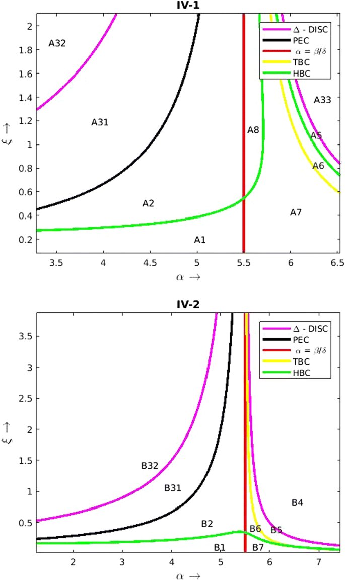
Additional food provided system (2.18)–(2.19) for \(\beta = 2.2, \ \delta = 0.4, \ \omega = 1.4654, 3.235, \ \& \ \gamma = 1.4388, 0.9052.\) The parameters chosen satisfy the condition IV-1, IV-2 in Table 1. This figure represents the division of control parameter space by the discriminant curve (DISC) (5.4), the prey elimination curve (PEC) (5.1), the Hopf bifurcation curve (HBC) (5.3), the transcritical bifurcation curve (TBC) (5.2) and the curve \(\alpha = \frac{\beta }{\delta }\)
Table 5 Global dynamics of the additional food provided system under Condition-IV

-
Region—V(V-1, V-2): The dynamics in this region V will be qualitatively similar to that of dynamics discussed in regions II, III and IV. A summary of the global dynamics of additional food provided system (2.18)–(2.19) under the Condition V can be found in Table 6 (Fig. 6).
Table 6 Global dynamics of the additional food provided system under Condition-V Fig. 6 
Additional food provided system (2.18)–(2.19) for \(\beta = 2.2, \ \delta = 0.4, \ \omega = 3.8618, 4.6912 \ \& \ \gamma = 1.6399, 0.94023.\) The parameters chosen satisfy the condition V-1, V-2 in Table 3. This figure represents the division of control parameter space by the discriminant curve (DISC) (5.4), the prey elimination curve (PEC) (5.1), the Hopf bifurcation curve (HBC) (5.3), the transcritical bifurcation curve (TBC) (5.2) and the curve \(\alpha = \frac{\beta }{\delta }\)

-
Region—VI(VI-1, VI-2): The dynamics in this region VI will be qualitatively similar to that of dynamics discussed in regions II, III and IV. A summary of the global dynamics of additional food provided system (2.18)–(2.19) under the Condition VI can be found in Table 7 (Fig. 7).
Table 7 Global dynamics of the Additional food provided system under Condition-VI Fig. 7 
Additional food provided system (2.18)–(2.19) for \(\beta = 2.2, \ \delta = 0.4, \ \omega = 4.894, 4.967 \ \& \ \gamma = 0.7216, 0.6166.\) The parameters chosen satisfy the condition VI-1, VI-2 in Table 3. This figure represents the division of control parameter space by the discriminant curve (DISC) (5.4), the prey elimination curve (PEC) (5.1), the Hopf bifurcation curve (HBC) (5.3), the transcritical bifurcation curve (TBC) (5.2) and the curve \(\alpha = \frac{\beta }{\delta }\)

The analysis presented above helps us to study some of the controllability aspects pertaining to the system (2.18)–(2.19) with respect to the control parameters \(\alpha\) and \(\xi\). The analysis suggests that, for an appropriate choice of additional food, the system can either be driven to a desired equilibrium level or to a limit cycle surrounding the desired equilibrium. If \((\tilde{x},\tilde{y})\) is the desired equilibrium state for the system, then \((\tilde{x},\tilde{y})\) can become an equilibrium point of the system (2.18)–(2.19), provided \(\alpha > 0\) and \(\xi > 0\) are chosen to satisfy
Let \(G(x) =\bigg (3\omega {x}^2(1 + \alpha \xi ) + 2x(1 -\omega \gamma (1 + \alpha \xi )) + (1 + \alpha \xi ) - \gamma \bigg ).\)
If \(G(\tilde{x}) <0\) then this equilibrium \((\tilde{x},\tilde{y})\) can be reached asymptotically. On the other hand, if \(G(\tilde{x}) > 0\) then the equilibrium would be unstable, as a result, solutions in the vicinity of this equilibrium approach a limit cycle surrounding \((\tilde{x},\tilde{y})\). For the given system parameters \(\beta , \delta\) and \(\gamma\) and the desired equilibrium \((\tilde{x},\tilde{y})\), the components of intersection of these two curves (5.5)–(5.6) give us the values of \(\alpha\) and \(\xi\) for which the considered system admits \((\tilde{x},\tilde{y})\) as its equilibrium.
The analysis also suggests that, for an appropriate choice of additional food, the equilibrium \((\tilde{x},\tilde{y})\) will remain as a saddle throughout its existence, provided, the values of \(\alpha\) and \(\xi\) are chosen to satisfy the following equations (for a given choice of \(\beta , \delta ,\)\(\gamma\) and \((\tilde{x},\tilde{y}),\)
6 Consequences of Providing Additional Food to Predators
It can be seen from the above discussions that the quality of additional food \(\alpha\) and its relation with respect to \(\frac{\beta }{\delta }\) plays a crucial role in determining the dynamics of the biosystem. As in Srinivasu et al. (2018), we characterize the additional food to be of high quality if \(\alpha < \frac{\beta }{\delta }\) and it is of low quality if \(\alpha > \frac{\beta }{\delta }\).
If the system (2.6)–(2.7) does not support the predator–prey coexistence initially (i.e., the system does not admit an interior equilibrium in the absence of additional food), then coexistence cannot be achieved by providing low quality additional food to predators. Whereas provision of additional food of high quality with supply level satisfying \(\frac{\delta (w\gamma ^2 + 1) - \gamma (\beta - \delta )}{(w\gamma ^2 + 1)(\beta - \alpha \delta )}< \xi < {\frac{\delta }{\beta - \delta \alpha }}\) brings coexistence into the system (refer Table 3).
On the other hand, if the system supports the stable coexistence of predator–prey, then on provision of additional food of high quality with supply level satisfying \(\xi > \frac{\delta }{\beta - \delta \alpha }\) eradicates the prey from the ecosystem. Also it possible to get in oscillations in the system for \(\xi\) satisfying the Hopf bifurcation Eq. (5.3) which can be removed on further increase of supply of additional food. In this scenario on provision of low quality additional food the second interior equilibrium \(E_3^*\) can be got into existence for supply of food for \(\xi > \frac{\delta (w\gamma ^2 + 1) - \gamma (\beta - \delta )}{(w\gamma ^2 + 1)(\beta - \alpha \delta )}\) and also the stable coexistence can be removed for the same supply level (refer Table 4).
If the system (2.6)–(2.7) is initially oscillatory then on provision of high quality additional food with supply level of \(\xi\) above the Hopf bifurcation curve (5.3) the system can be stabilized. In this case on provision of low quality additional food we have multiple things happening. For supply level of \(\xi\) above the Hopf bifurcation curve (5.3) the system can be stabilized. For \(\xi > \frac{\delta (w\gamma ^2 + 1) - \gamma (\beta - \delta )}{(w\gamma ^2 + 1)(\beta - \alpha \delta )},\) the axial equilibrium \(E_1^*\) can be made stable and a homoclinic orbit can be got into existence. Also the second interior equilibrium \(E_3^*\) can be got into existence (refer Table 5).
Now let us consider the case where initially the axial equilibrium \(E_1^*\) is stable and there are oscillations in the system. Then on provision of low quality additional food for supply level \(\xi > \frac{-\beta + (1+2\sqrt{w})\delta }{2\sqrt{w}(\beta - \delta \alpha )},\) the interior equilibria vanish. While on the other hand provision of additional food of high quality leads to very interesting scenarios. For supply level \(\xi > \frac{\delta (w\gamma ^2 + 1) - \gamma (\beta - \delta )}{(w\gamma ^2 + 1)(\beta - \alpha \delta )},\) the axial equilibrium \(E_1^*\) can be made to loose its stable nature and the second interior equilibria \(E_3^*\) can be made to vanish. Also, for supply level \(\xi\) above the Hopf bifurcation curve (5.3) the oscillations can be removed and stable coexistence can be got in (refer Table 6).
Finally let us consider the case where initially the axial equilibrium \(E_1^*\) is stable and there is stable coexistence of predator–prey. Then on provision of low quality additional food for supply level \(\xi > \frac{-\beta + (1+2\sqrt{w})\delta }{2\sqrt{w}(\beta - \delta \alpha )},\) the interior equilibria vanish. In this case on provision of high quality additional food we have interesting things happening. For supply level \(\xi > \frac{\delta (w\gamma ^2 + 1) - \gamma (\beta - \delta )}{(w\gamma ^2 + 1)(\beta - \alpha \delta )},\) the axial equilibrium \(E_1^*\) can be made to loose its stable nature and the second interior equilibria \(E_3^*\) can be made to vanish. Also, for supply level \(\xi\) above the Hopf bifurcation curve (5.3) oscillations can be got into the system and after the second Hopf bifurcation stable coexistence can be got in (refer Table 7).
7 Time Optimal Control Studies
To overcome the limitations of asymptotics, we do the time optimal control studies in this section.
7.1 Existence of Optimal Solution
In this subsection we establish the existence of optimal solution.
Let the initial state and the desired terminal state of the system (2.18)–(2.19) be \((x_0,y_0)\) and \((\bar{x},\bar{y}).\) Our goal is to drive the system \((x_0,y_0)\) to \((\bar{x},\bar{y})\) in minimum time. Here the control parameters \(\alpha\) and \(\xi\) can vary in \([\alpha _{min} ,\alpha _{max}]\) and \([\xi _{min} ,\xi _{max}]\) respectively. Thus the problem can be considered as a time optimal control problem with \((\alpha (t), \xi (t))\) as control variables which can be stated as follows:
Clearly, the above problem (7.1) is a Mayer problem of minimum time (Cesari 1983). We now establish the existence of an optimal solution for (7.1) using Fillipov existence theorem for Mayer problem (Cesari 1983). Comparing the above optimal control problem with that of General form of Mayer time optimal control problem (Cesari 1983), we have \(n = 2, m = 2\) and \(X(t) = (x(t),y(t)), u(t) = (\alpha (t),\xi (t))\) with \(f(t,X(t),u(t)) = (f_1(t,x,y,\alpha ,\xi ), f_1(t,x,y,\alpha ,\xi ))\) where
The boundary conditions are \(e[x]= (0,x_0,y_0, T, \overline{x}, \overline{y}).\)
Here, \(\Omega = \bigg ((x,u=(\alpha ,\xi ))| (x,u)\) is an admissible pair of the system (2.18)–(2.19)\(\bigg )\).
Theorem 7.1
If\(\Omega\)is non-empty then the time optimal control problem (7.1) has an absolute minimum.
Proof
We prove this result by showing that all the conditions of Fillipov Existence theorem are satisfied. We see that for \(\alpha < \frac{\beta \xi -\delta }{\delta \xi }\) any solution initiating in the positive quadrant reaches y-axis in a finite time. Hence, we can assume that the set A(the set of admissible equilibria of (7.1)) subset of \(\mathbb R ^{1+2}\) to be compact. To justify the existence of optimal solution it is sufficient to show that for \((t,x,y) \in A\) the sets
\(Q(t,x,y) = \bigg ((J_1,J_2)| J_1 = f_1(t,x,y,\alpha ,\xi ), J_2 = f_2(t,x,y,\alpha ,\xi ), \alpha \in [\alpha _{min},\alpha _{max}], \xi \in [\xi _{min} ,\xi _{max}]\bigg )\) are convex, where
For, Let us consider
This implies that
Hence, we have,
The above linear relation between \(J_1\) and \(J_2\) imply that Q(t, x, y) are segments that are convex. Thus if \(\Omega\) is a non empty then the time optima control problem (7.1) has an absolute minimum. \(\square\)
7.2 Characterizations of Optimal Control Functions
In this subsection we characterize the optimal control functions using the Pontryagins maximum principle (Liberzon 2012).
We first define Hamiltonian for the system (7.1) as,
Here \(\lambda = (\lambda _1, \lambda _2 )\) is the adjoint variable.
Theorem 7.2
Let\(\alpha ^*\)and\(\xi ^*\)be optimal control functions and\(x^*\)and\(y^*\)be corresponding sate variables of the control problem (7.1). Then there exists adjoint variable\(\lambda =(\lambda _1,\lambda _2) \in \mathbb R^2\)which satisfy the following canonical equations.
With transversality conditions\(\lambda _1(T) = 0 = \lambda _2(T)\).
The corresponding optimal controls \(\alpha ^{*}\) and \(\xi ^*\) are given as
Proof
Let \(\alpha ^*\) and \(\xi ^*\) be the given optimal controls and \(x^*\), \(y^*\) be corresponding state variables of system (7.1) that minimizes cost functional in (7.1). Then by Pontryagins maximum principle, there exists adjoint variables \(\lambda _1\) and \(\lambda _2\) (costate vector) which satisfy the canonical equations, \(\frac{d\lambda _1}{dt}= -\frac{\partial H}{ \partial \alpha }\) and \(\frac{d\lambda _2}{dt}= -\frac{\partial H}{ \partial \xi }\) with transversality conditions \(\lambda _1(T)= 0 =\lambda _2(T).\) Here Hamiltonian H is given as in (7.2).
Hence,
which imply that
Now from optimality condition, we have,
\(\frac{\partial H}{\partial u_i}=0\) at \(u_1= \alpha ^*\) and \(u_2= \xi ^*\)
Thus we get \(\alpha ^* =\frac{\lambda _2 \beta (x + (1 + \omega x^2))}{\lambda _2 \beta x - \lambda _1 x}\) and \(\xi ^*= \frac{\lambda _1 x - \lambda _2\beta x}{\lambda _2 \beta (x + (1 + \omega x^2))}.\)
Using Characteristics of Control space U and above discussion the optimal controls \(\alpha ^*\) and \(\xi ^*\) are given as in (7.3) and (7.4). It is observed that the optimal controls depend on prey population alone. \(\square\)
8 Discussion and Conclusions
In this article we study the additional food provided predator–prey systems where Holling type IV functional response has been assumed for the predators (incorporating the inhibitory effect of the prey) and also predators are assumed to be non optimal foragers. Initially we discuss the positivity, boundedness and uniform persistence of the system (2.6)–(2.7). We later discuss the local and global dynamics. The quality of the additional food is characterized by its nutritive value and handling time. It is termed as low quality if the maximum growth rate of the predator due to consumption of additional food is less than the natural death rate of the predator and it is of high quality if the above mentioned relation reverses. The system analysis bifurcates the qualitative study into two significant cases that depend on the quality of the additional food as presented below.
Case 1
(low quality additional food) In this case, we clearly have either the handling time for the predator of the additional food to be higher or the nutritive value of the additional food to be lower than that of the target prey.
In this case we find that, if initially the predators are unable to survive due to the group defense (inhibitory effect) of the prey, then providing any amount of additional food of low quality to predators can not bring in coexistence between the prey and the predator. This is due to the fact that, if in the absence of additional food itself the predators are not able to predate on the prey, then providing additional food of lower quality will not improve the sustenance of the predators. Moreover the presence of additional food distracts the predators (from the target prey) which are time limited. So in this situation controlling the prey using biological means cannot be achieved.
On the other hand if the system supports the stable coexistence of predator–prey, then on provision of additional food the stable coexistence can be removed which can be attributed to the low quality nature of the additional food supplied. If initially the system is oscillatory then by providing additional food with relatively higher handling time it is possible to compress these oscillations and even eliminate them bringing in the stable coexistence. In the case wherein the system is initially prey dominated and there are oscillations, then on the supply of low quality additional food the oscillations can be made to die out but stable coexistence of predator–prey cannot be brought in. The system continues to remain prey dominated because of the inhibitory effect of the prey. Finally we consider the case where the system is initially prey dominated in one part and there is stable coexistence of the predator–prey in the other remaining part of the system. Then on provision of low quality additional food the stable coexistence can be removed and the biosystem can be made prey dominated. Again this can be attributed to the low quality nature of the additional food.
These results supports the inferences in Putman and Staines (2004) which states that “the red deerCervus elaphusmay develop a reliance on the food supplement provided, reducing intake of natural forages to near zero; where feed provided is less than 100 percent of daily requirement, these animals may regularly lose, rather than gain condition. Also, it is stated that provision of low quality food supplements such as grain, root crops which are deficient in fiber may adversely affect the water balance of predators. It has been observed that winter feeding did not produce calves with greater birth weights than those reported for animals which are not given supplementary feed.” Also in Glaser (1983) it has been mentioned that “Weight of supplementally fed stags in contrast showed significant decrease, with mean weights of adult stags, male calves coming down.”
Case 2
(high quality additional food) If the system does not support coexistence between the prey and predator in the absence of additional food due to the inhibitory effect of the prey, then coexistence can be brought into the system by providing additional food of high quality. This coexistence can continue to remain with increased additional food level till the prey vanishes from the system.
On the other hand if the system supports the stable coexistence of predator–prey, then on provision of additional food, the stable coexistence can continue to remain till the prey vanishes from the system or this stable coexistence can depend on the quality and quantity of the additional food. If the quality of additional food is greater than a critical \(\alpha ^{'}\) then the stable coexistence will continue to remain with increased additional food level till the prey vanishes from the system.
In case if the quality of the additional food is less than the said critical value \(\alpha ^{'},\) provision of additional food, induces oscillations into the system. With further increase in the quantity of additional food, the system once again stabilizes at low prey equilibrium density. While retaining the stability, this low equilibrium value of the prey continues to decrease with increase in the additional food quantity and the prey goes to extinction for a specific level of additional food supply. This behavior may be attributed to the fact that provision of additional food of very high quality increases the fecundity of the predators which in turn increases the predation pressure on the prey. Also, the abundance of predators in the environment and their dependence on both additional food as well as prey brings in oscillations into the system. Beyond a certain level of food supply, the system gets stabilized again. Further increase in the quantity of additional food increases the predators which in turn leads to the extinction of the prey population. Thus the prey can be controlled biologically in this case.
In the other case if the system admits an unstable interior equilibrium initially, then on supply of additional food, on increase in the quantity the oscillations in the system can be subdued and stable coexistence can be achieved. Continuous supply of additional food further, will extinct the prey, thereby achieving the biological control. The initial oscillations in the system can be attributed to the relatively high carrying capacity of the system with respect to the earlier cases. Due to the continuous supply of high quality additional food from hereon, the predators fecundity and ferocity increases thereby getting the stable coexistence. As in the earlier situation further increase in the quantity of additional food leads to the extinction of the prey population.
We now consider the case when the system is initially prey dominated in one part and admits oscillations in the other remaining part. Then on supply of additional food the system can be made non prey dominated and on further provision even the oscillations can be removed getting in the stable coexistence of the predator–prey. Continuous supply of additional food further, will extinct the prey. Thus the system can be biologically conserved in this case which can be attributed to the high quality additional food. Finally in the case wherein the system is initially prey dominated in one part and admits stable coexistence of predator–prey in the other remaining part, we observe that on provision of additional food the system can be made non prey dominated. On further provision of additional food, this stable coexistence continues to remain till the prey gets extinct or oscillations can get induced into the system. With further increase in the quantity of additional food, the system once again stabilizes at low prey equilibrium density. Continuous supply of additional food further, will extinct the prey. This behaviours can be attributed to the high quality nature of additional food.
These results supports the inferences in Putman and Staines (2004) which states that “good quality of additional food supplements such as hay if providedad libitumwill be sufficient to maintain its body condition over winter.” In Kozak (1994, 1995) it is stated that “In experimental conditions, food supplemented wapitit hinds maintained body condition and body mass overwinter better than unsupplemented animals. Food supplementation over winter could increase milk production of lacting hinds thus increasing calf growth rates.”
We finally study time optimal control problems to overcome the limitations of asymptotics. It is proved that the optimal controls depend on prey population alone. We conclude that with provision of additional food as a tool, a predator–prey system (with inhibitory effect of the prey towards predator) can be controlled and steered to a desirable state. With appropriate choice on the quality and quantity of additional food, the predator–prey system can be stabilized at a state with low prey and high predator densities or high prey and low predator densities. It is also possible to eliminate either of the interacting species through provision of suitable additional food to predators. This analysis offers eco friendly strategies to manage a predator–prey system. The vital role of the quality and quantity of the additional food in the system dynamics cautions the manager on the choice of the additional food for realizing the goal in the biological conservation programme. An arbitrary choice of the additional food can result in completely opposite results to the desired ones.
References
Birkhoff G, Rota GC (1989) Ordinary differential equations. John Wiley & Sons, Hoboken
Butler GJ et al (1986) Uniformly persistent systems. Proc Am Math Soc 96:425–429
Cesari L (1983) Optimization—theory and applications: problems with ordinary differential equations, applications of mathematics series, vol 17. Springer, New York
Collings JB (1997) The effects of the functional response on the bifurcation behavior of a mite predator prey interaction model. J Math Biol 36:149–168
David S (1995) Hik: does risk of predation influence population dynamics? Evidence from the cyclic decline of Snowshoe Hares. Wildl Res 22:115–129
Elkinton Joseph S et al (2004) Effects of alternative prey on predation by small mammals on gypsy moth pupae. Popul Ecol 46:171–178
Freedman HI, Wolkowicz GSK (1986) Predator–prey systems with group defence: the paradox of enrichment revisited. Bull Math Biol 48:493–508
Glaser O (1983) Wintergattermanagement: Fallstudien in obsersteirischen rotwildgattern. Diploma Thesis. Agricultural University of Vienna
Harmon JP (2003) Indirect interactions among a generalist predator and its multiple foods, Ph.D Thesis. University of Minnesota, St. Paul, MN
Holt RD (1984) Spatial heterogeneity, indirect interactions, and the coexistence of prey species. Am Nat 124:377–406
Huang JC, Xiao DM (2004) Analysis of bifurcations and stability in a predator–prey system with holling type-IV functional response. Acta Math Appl Sin Engl Ser 20:167–178
Huang J et al (2014) Bifurcations in a predator–prey system of Leslie type with generalized Holling type III functional response. J Differ Eq 257:1721–1752
Kar TK (2012) Bapan Ghosh: sustainability and optimal control of an exploited prey predator system through provision of alternative food to predator. BioSystems 109:220–232
Kot M (2001) Elements of mathematical ecology. Cambridge University Press, Cambridge
Kozak HM et al (1994) Supplemental winter feeding. Rangelands 16:153–156
Kozak JM et al (1995) Winter feeding, lactation and calf growth in farmed wapiti. Rangelands 17:116–120
Liberzon D (2012) Calculus of variations and optimal control theory: a concise introduction. Princeton University Press, Princeton
Putman RP, Staines BW (2004) Supplementary winter feeding of wild red deer Cervus elaphus in Europe and North America: justifications, feeding practice and effectiveness. Mamm Rev 34:285–306
Redpath SM et al (2001) Does supplementary feeding reduce predation of red grouse by hen harriers? J Appl Ecol 38:1157–1168
Sahoo B, Poria S (2014) Effects of supplying alternative food in a predator–prey model with harvesting. Appl Math Comput 234:150–166
Sahoo B, Poria S (2015) Effects of additional food in a delayed predator–prey model. Math Biosci 261:62–73
Srinivasu PDN et al (2007) Biological control through provision of additional food to predators: a theoretical study. Theor Popul Biol 72:111–120
Srinivasu PDN, Vamsi DKK, Aditya I (2018) Biological conservation of living systems by providing additional food supplements in the presence of inhibitory effect: a theoretical study using predator–prey models. Differ Eq Dyn Syst 26:213–246
Zhu H et al (2002) Bifurcation analysis of a predator–prey system with nonmonotonic function response. SIAM J Appl Math 63:636–682
Acknowledgements
The authors dedicate this paper to the founder chancellor of Sri Sathya Sai Institute of Higher Learning, Bhagawan Sri Sathya Sai Baba. The corresponding author also dedicates this paper to his loving elder brother D. A. C. Prakash who still lives in his heart. The second author acknowledges the partial financial support from SAI-DAMCS fund of SSSIHL for this work.
Author information
Authors and Affiliations
Corresponding author
Additional information
Publisher's Note
Springer Nature remains neutral with regard to jurisdictional claims in published maps and institutional affiliations.
Rights and permissions
About this article

Cite this article
Vamsi, D.K.K., Kanumoori, D.S.S.M. & Chhetri, B. Additional Food Supplements as a Tool for Biological Conservation of Biosystems in the Presence of Inhibitory Effect of the Prey. Acta Biotheor 68, 321–355 (2020). https://doi.org/10.1007/s10441-019-09371-x
Received:
Accepted:
Published:
Issue Date:
DOI: https://doi.org/10.1007/s10441-019-09371-x