Topological design for mechanical metamaterials using a multiphase level set method

Abstract

Metamaterials usually refer to artificially engineered composites with unusual properties that cannot be easily found in nature. This paper will develop a topological shape optimization method for design of mechanical metamaterials of thermoelastic micro-structured composites, which integrates numerical homogenization method with a multi-phase level set method (MPLSM). The homogenization method is applied to evaluate the effective macroscopic properties of a periodic microstructure, while the MPLSM will be utilized to implement shape and topology evolutions of the microstructure. A multi-phase level set representation model is established to describe the boundaries of the multi-material microstructure using a combination of all level set functions, without overlaps and empties. The Hamilton-Jacobi partial differential equation-based topological shape optimization problem will be transformed to a generalized size optimization problem. Typical numerical examples are used to demonstrate the effectiveness of the proposed method for designing metamaterials with expected and extreme thermal expansion coefficients.

1 Introduction

Metamaterials are actually artificial composite materials engineered to have unconventional properties caused by local resonance phenomenon, which usually consists of arrays of periodically configured microstructures fashioned with conventional materials. Metamaterials gain their fascinating properties from the periodic microstructures rather than from their composition. Thus the layout including the geometric shape and topology of the microstructure will be of great importance for triggering the unusual properties of the metamaterials. Due to the exotic properties, metamaterials are experiencing popularity in a number of new and emerging areas. Several types of micro- and nano-structured metamaterials have been developed, including electromagnetic metamaterials (Smith et al. 2004; Sihvola 2007), mechanical or elastic metamaterials (Lakes 1987; Milton 1992; Evans and Alderson 2000) and acoustic metamaterials (Chen and Chan 2007). This paper focuses on metamaterial designs to achieve extreme or desired thermoelastic properties using topological shape optimization approach with a multi-phase level set method.

The expansion and contraction of materials and structures must be considered in engineering applications, when changes in dimension as a result of temperature. The thermal expansion due to temperature changes is of interest from both a technological and fundamental standpoint. The thermal expansion coefficient of materials can be defined as the change of matter in volume with respect to a change in temperature. Artificial composite materials with unusual thermal expansion coefficients are rare in nature, such as materials with zero thermal and negative thermal expansion coefficients, which play an important role in engineering. The zero thermal expansion coefficients denote the dimension of a structure keeps unchanged with temperature changes. A material with negative thermal expansion coefficient has the counterintuitive property that contracts when increasing temperature within certain temperature ranges. For example, the thermal expansion coefficient of water becomes negative below 277.15 K (4 C), and pure silicon has a negative thermal expansion coefficient for temperatures between 18 and 120 K. Currently, there is still a demand for advanced design methods to create micro-structured thermoelastic composites.

Topology optimization (Bendsøe and Sigmund 2003) has been identified as one of the most promising structural optimization methods, which can establish an overall framework of the conceptual design without prior knowledge of a design. Topology optimization can be regarded as a numerical process that iteratively distributes a prescribed amount of material inside a fixed design domain, so as to determine the best layout of the material until the objective function is optimized subject to constraints. Several topology optimization methods have been developed in the field, including the homogenization method (Bendsøe and Kikuchi 1988), the evolutionary structural optimization (ESO) method (Xie and Steven 1993), the Solid Isotropic Material with Penalization (SIMP) method (Zhou and Rozvany 1991; Bendsøe and Sigmund 1999), the nodal density-based interpolation (PDI) scheme (Guest et al. 2004; Kang and Wang 2011; Luo et al. 2013), and the level set-based method (LSM) (Sethian and Wiegmann 2000; Wang et al. 2003; Allaire et al. 2004). These methods have been widely applied to the computational design of a broad range of structures and materials, including the micro- and nanostructured metamaterials, such as (Larsen et al. 1997; Diaz and Sigmund 2010; Zhou et al. 2011; Lu et al. 2013; Otomori et al. 2012; Wang et al. 2014; Xie et al. 2014). Particularly, the inverse homogenization method (IHM) (Sigmund 1994) has been combined with other approaches to create various microstructures for metamaterials with desired properties or extreme properties, e.g. (Sigmund and Torquato 1997; Sigmund 2000; Guest and Prévost 2007; Huang et al. 2013). To achieve the optimal design of multifunctional structures, particularly materials with unusual thermal expansion coefficients, a multiphase design strategy is required for topology optimization method. Hence, choosing a proper topological description model is an essential issue for the topology optimization of metamaterials involving multiple phases (Sigmund 2001; Luo et al. 2010; Tavakoli and Mohseni 2014; Gao and Zhang 2011; Wang et al. 2015; Allaire et al. 2014). In the case of multiphase topology optimization problems the challenge is mainly related to the mathematical structure of design space. Till now, a few multiphase models for describing a microstructure have been developed. For instance, Bendsøe and Sigmund (Sigmund 2001) proposed a mixture rule for multi-material models based on SIMP material density distribution approach, and has been applied to multi-physics compliant actuators (Sigmund 2001; Luo et al. 2010) and multi-material structures (Tavakoli and Mohseni 2014; Gao and Zhang 2011). Another implicit representation method, namely the phase field method, which represent the domain and interfaces by using a set of field variables, were also applied to multi-material design problems (Zhou and Wang 2007; Tavakoli 2014).

After the works of (Sethian and Wiegmann 2000; Wang et al. 2003; Allaire et al. 2004), several different and alternative LSMs, e.g. (Wang and Wang 2004; Xia et al. 2006; Yamasaki et al. 2010; Dijk et al. 2012; Zhou and Wang 2012; Dunning and Kim 2013; Luo et al. 2008a, 2009, 2012; Belytschko et al. 2003), have been developed within the standard framework of LSM (Sethian 1999; Osher and Fedkiw 2002) for different topology optimization problems (Dijk et al. 2013). In particular, the parametric level set method (PLSM) (Luo et al. 2007, 2008b) has shown its ability as a powerful method for topological shape optimization of structural and material designs, e.g. (Wang et al. 2015, 2016; Li et al. 2015). The PLSM can remain the favorable features of most LSMs while avoid the difficulties of their standard forms, and enable the direct application of more efficient gradient-based optimization algorithms in LSMs. In this paper, a multiphase topology description model, based on a Multi-Material Level Set (MM-LS) topological description model (Wang et al. 2015), is extended for topological design of multiphase microstructure.

In the MM-LS topological description model, higher-order surfaces are used to implicitly represent the structural boundary as zero level sets, and the material property at any point in the design domain is calculated according to a combination rule of different level set functions. Thus, a total number of I level set functions are used to indicate I + 1 distinct phases, including I solid phases and one void phase. Aside from topology description, it has been shown that this level set based method can remain the advantages of traditional level set method in terms of smooth boundary and distinct interface, and can track the changes of shapes and topologies by merging and splitting of the moving boundaries. The drawback of the level set based methods would be the dependency of the optimized topologies to the initial designs.

This paper focuses on the design of thermoelastic metamaterials using a level-set topology optimization method, by applying the MM-LS topology description model. The numerical homogenization method, to determine the effective properties of the composite, is combined with the PLSM to implement the inverse design of composite materials. The proposed level set method will be employed to optimize the shape and topology of the microstructure. It is noted that multi-material composite can often gain extraordinary properties beyond those of their individual components. Several numerical examples will be used to demonstrate the effectiveness of the proposed method for the design of multi-phase composite materials.

2 A multiphase level set method using CSRBFs

2.1 Level-set boundary representation

In level-set based topology optimization methods, one of the key concepts is to implicitly embed the initial position of the structural boundary as the zero level set of a higher-dimensional level set function. For example, if Φ(x) is defined as a Lipschits continuous level set function over a reference domain D, Fig. 1 shows a two-dimensional (2D) boundary of the structure that is represented by the three-dimensional (3D) level set surface, where the level set function is used to uniformly denote the different material phases inside the reference domain (Sethian 1999; Osher and Fedkiw 2002), as follows:

Fig. 1

2D boundary representation using 3D level set surface

$$ \left\{\begin{array}{lll}\varPhi \left(\mathbf{x}\right)>0\hfill & \forall \mathbf{x}\in \varOmega \backslash \partial \varOmega \hfill & \left(\mathrm{Solid}\kern0.5em \mathrm{region}\right)\hfill \\ {}\varPhi \left(\mathbf{x}\right)=0\hfill & \forall \mathbf{x}\in \partial \varOmega \hfill & \left(\mathrm{Boundary}\right)\hfill \\ {}\varPhi \left(\mathbf{x}\right)<0\hfill & \forall \mathbf{x}\in D\backslash \left(\varOmega \cup \partial \varOmega \right)\hfill & \left(\mathrm{Void}\right)\hfill \end{array}\right. $$

(1)

To enable the dynamic motion, the pseudo-time t is introduced into the level set function Φ(x). Then the evolution of the level set function Φ(x, t) is linked to the propagation of the boundary located at Φ(x) = 0, leading to the following first-order Hamilton-Jacobi partial differential equation (H-J PDE) (Sethian 1999; Osher and Fedkiw 2002) by differentiating Φ(x, t) on both sides with respect to t:

$$ \begin{array}{ccc}\hfill \frac{\partial \varPhi \left(\mathbf{x},t\right)}{\partial \mathrm{t}}-{\mathbf{v}}_{\mathrm{n}}\left|\nabla \varPhi \left(\mathbf{x},t\right)\right|=0,\hfill & \hfill \mathrm{where}\hfill & \hfill {\mathbf{v}}_{\mathrm{n}}=\mathbf{v}\cdot \mathbf{n}=\left(\frac{\mathrm{d}\mathbf{x}}{\mathrm{d}t}\right)\cdot \left(-\frac{\nabla \varPhi }{\left|\nabla \varPhi \right|}\right)\hfill \end{array} $$

(2)

It is noted that only the normal velocity component v _n contributes to shape evolution of the boundary. Hence, moving boundary along the normal direction n is equivalent to transporting Φ(x, t) by solving the H-J PDE with finite difference schemes on a fixed Eulerian rectilinear grid.

As aforementioned, the numerical solution of the H-J PDE requires appropriate choice of finite difference schemes, CFL condition, re-initializations and velocity extension methods, which involve complicated numerical procedures and require excessive amount of computational efforts, and thus limit the utility of LSMs. Moreover, due to the prohibition of nucleating new holes inside the material domain, the final design strongly depends on the initial guess.

2.2 Parameterization/Interpolation of level set surface

This paper will extend the parametric level set method developed by (Luo et al. 2007, 2008b) to the computational design of thermoelastic metamaterials. The core concept behind this method is to implement the discretization or parameterization of the implicit level-set surface through the interpolation of a known set of compactly supported radial basis functions (CSRBFs) (Wendland 2006). The level set function (surface) can be described by the interpolation of CSRBFs at a set of pre-specified knots fixed in the whole design domain, as follows:

$$ \varPhi \left(\mathbf{x},t\right)=\boldsymbol{\upvarphi} \left(\mathbf{x}\right)\mathbf{c}(t)={\displaystyle \sum_{i=1}^N{\varphi}_i\left(\mathbf{x}\right){c}_i(t)} $$

(3)

The vectors of the CSRBFs and the corresponding expansion coefficient are given by

$$ \boldsymbol{\upvarphi} \left(\mathbf{x}\right)=\left[{\varphi}_1\left(\mathbf{x}\right),{\varphi}_2\left(\mathbf{x}\right),\dots, {\varphi}_N\left(\mathbf{x}\right)\right]\in {\mathbb{R}}^N $$

(4)

$$ \mathbf{c}(t)={\left[{c}_1(t),{c}_2(t),\dots, {c}_N(t)\right]}^T\in {\mathbb{R}}^N $$

(5)

where x denotes the position of any knot, i = 1,2,…,N, and N is the total number of the CSRBF knots.

In the numerical implementation, an appropriate radius of support is required for CSRBFs, in order to ensure non-singularity and the computational efficiency of the interpolant (Wendland 2006). The interpolation leads to a separation of the space and time of the level set function, in which the CSRBFs are spatial only while the expansion coefficients are time dependent. Thus, the decoupling of the H-J PDE is given by

$$ \boldsymbol{\upvarphi} \left(\mathbf{x}\right)\frac{d\mathbf{c}(t)}{dt}-{\mathbf{v}}_{\mathrm{n}}\left|\nabla \boldsymbol{\upvarphi} \left(\mathbf{x}\right)\mathbf{c}(t)\right|=0 $$

(6)

It can be found that v _n is related to the time derivative of the expansion coefficients, as follows:

$$ \begin{array}{ccc}\hfill {\mathbf{v}}_{\mathrm{n}}=\frac{\boldsymbol{\upvarphi} \left(\mathbf{x}\right)}{\left|\nabla \boldsymbol{\upvarphi} \left(\mathbf{x}\right)\mathbf{c}(t)\right|}\overset{.}{\mathbf{c}}(t),\hfill & \hfill \mathrm{where}\hfill & \hfill \overset{.}{\mathbf{c}}(t)=\frac{d\mathbf{c}(t)}{dt}\hfill \end{array} $$

(7)

From the above equation, it can be found that all the terms involved in v _n will actually by evaluated at the knots over the whole domain. Thus, v _n will be naturally applied to the entire design domain. In this way, the H-J PDE has been changed into a system of algebraic equations, and therefore the original topological optimization is transformed into an easiest size optimisation, in which the only unknowns are the expansion coefficients c(t) that are actually defined as the design variables. Hence, the propagation of the boundary and the evolvement of the level set function, as well as the changes of the shape and topology of the structure are just a problem of updating c(t) using appropriate optimization algorithms.

3 Topology optimization for multi-phase thermoelastic composites

In this Section, for simplicity but without losing any generality, we will use three-phase material structure to describe the numerical procedure for topology optimization of thermoelastic metamaterials. The design domain of three-phase material microstructure consists of two different solid material phases and void which is filled with a very weak material phase. Firstly, the numerical homogenization method (Guedes and Kikuchi 1990; Andreassen and Andreasen 2014) is applied to evaluate the effective properties of the microstructure. Secondly, the proposed multi-phase level set method will be employed to achieve the optimized shape and topology of the microstructure, in order to achieve optimal design of metamaterials with prescribed effective properties.

3.1 A multi-material level set description model

To solve the multi-material design problem using the parametric level set method, we will propose a level set representation model for the multiphase design domain of microstructure, based on (Wang et al. 2015), in which each individual phase was represented via a simple artificial mixture assumption of all level set functions.

This paper introduces the concept of multi-phase material representation model in SIMP (Sigmund 2001; Gibiansky and Sigmund 2000) into the level set methods. The tensors of elasticity C and thermal expansion coefficient α at point x for design problem with two solid phases can be written as a combination of the two level set functions Φ ₁ and Φ ₂ as:

$$ {C}_{ijkl}\left(\mathbf{x},\varPhi \right)=H\left({\varPhi}_1\right)\left(1-H\left({\varPhi}_2\right)\right){C}_{ijkl}^1+H\left({\varPhi}_1\right)H\left({\varPhi}_2\right){C}_{ijkl}^2 $$

(8)

$$ {\alpha}_{ij}\left(\mathbf{x},\varPhi \right)=\left(1-H\left({\varPhi}_2\right)\right){\alpha}_{ij}^1+H\left({\varPhi}_2\right){\alpha}_{ij}^2 $$

(9)

where i, j, k, l = 1, 2,…, d (d is the dimension of space). The two solid material phases have different elastic moduli and thermal expansion coefficients, described by C ¹ _ijkl and C ² _ijkl , and α ¹ _ij and α ² _ij . H is the Heaviside function, given as follows:

$$ \mathrm{H}\left(\varPhi \left(\mathbf{x}\right)\right)=\left\{\begin{array}{cc}\hfill \theta \hfill & \hfill \mathbf{x}<-\varDelta \hfill \\ {}\hfill \frac{3\left(1-\theta \right)}{4}\left(\frac{\varPhi \left(\mathbf{x}\right)}{\varDelta }-\frac{\varPhi {\left(\mathbf{x}\right)}^3}{3{\varDelta}^3}\right)+\frac{1+\theta }{2}\hfill & \hfill -\varDelta \le \mathbf{x}<\varDelta \hfill \\ {}\hfill 1\hfill & \hfill \mathbf{x}\ge \varDelta \hfill \end{array}\right. $$

(10)

where θ is a small positive number used to ensure the non-singularity of the stiffness matrix in the numerical implementation, and Δ is the width in the numerical approximation for the Heaviside function. The Heaviside function is actually smoothed to facilitate the calculation of the first-order derivatives of the objective function. The smoothed Heaviside function can smear the boundaries of level sets and a too large value of Δ will result in numerical errors for the boundaries between phases. Based on our experience, θ = 0.0001 and Δ = 0.1 in this study.

With the discretization of finite elements, Η(Φ ₁) can be used to indicate whether an element is solid or void, namely Η(Φ ₁) = θ being a void element while Η(Φ ₁) =1 being a solid element. Based on the definition of Η(Φ ₁) =1, Η(Φ ₂) is further used to distinguish if the solid element is occupied by the solid material 1 or by the solid material 2. Thus, the combination of Η(Φ ₁) =1 and Η(Φ ₁) = θ represents an element with the solid material 1, and the mixture of Η(Φ ₁) =1 and Η(Φ ₁) =1 is the solid material 2. In this way, each material phase in the design domain can be uniquely represented by the above model.

3.2 Effective material properties using numerical homogenization method

Homogenization theory is based on the asymptotic expansion of the governing equation, enabling a separation of the macro- and microscopic length scales, so as to extract homogeneous effective material properties from heterogeneous media. To evaluate the effective thermal expansion properties of the composite using the homogenization method, we assume that (1) the metamaterials consist of an assembly of microstructures (base cell), as shown in Fig. 2; (2) the size of the periodic microstructure is much smaller than the characteristic size of composite to allow scale-decomposition; and (3) the effective homogenized property of the composite can be predicted by a single unit cell.

Fig. 2

Schematic of multi-material periodic structures with microstructures

In this study, the topological shape optimization will be performed within the unit cell Y that is regarded as the design domain. The period Y is assumed to be very small in comparison with the dimension of the overall domain Ω of the medium. According to the theory of homogenization, the effective homogenized properties of the thermoelastic composite material can be computed as follows:

$$ {C}_{ijkl}^{\mathrm{H}}=\frac{1}{\left|Y\right|}{\displaystyle {\int}_Y{C}_{pqrs}\left({\varepsilon}_{pq}^{0(ij)}-{\varepsilon}_{pq}^{*(ij)}\right)\left({\varepsilon}_{rs}^{0(kl)}-{\varepsilon}_{rs}^{*(kl)}\right)\mathrm{d}Y} $$

(11)

$$ {\beta}_{kl}^{\mathrm{H}}=\frac{1}{\left|Y\right|}{\displaystyle {\int}_Y{C}_{pqrs}\left({\alpha}_{pq}-{\varepsilon}_{pq}^{\alpha}\right)\left({\varepsilon}_{rs}^{0(kl)}-{\varepsilon}_{rs}^{*(kl)}\right)\mathrm{d}Y} $$

(12)

$$ {\alpha}_{ij}^{\mathrm{H}}={\left({C}_{ijkl}^{\mathrm{H}}\right)}^{-1}{\beta}_{kl}^{\mathrm{H}} $$

(13)

where C ^H _ijkl is the effective elasticity tensor, β ^H _kl is the effective thermal stress tensor, and α ^H _ij is the effective thermal strain tensor; |Y| is the volume (area) of the cell; C _pqrs is the locally varying elasticity tensor; ε ⁰ is the prescribed macroscopic strain field including the unit strain in the horizontal and vertical directions and the unit shear strain. In the above equations:

• (1) The locally varying strain fields ε ^* (kl) _rs are defined by

  $$ {\varepsilon}_{rs}^{*(kl)}={\varepsilon}_{rs}^{*}\left({\chi}^{kl}\right)=\frac{1}{2}\left(\frac{\partial {\chi}_r^{kl}}{\partial {y}_s}+\frac{\partial {\chi}_s^{kl}}{\partial {y}_r}\right) $$

  (14)

  in which the displacement fields χ ^kl can be obtained by solving the following equation

  $$ \begin{array}{cc}\hfill {\displaystyle {\int}_Y{C}_{pqrs}{\varepsilon}_{pq}(v){\varepsilon}_{rs}^{*}\left({\chi}^{kl}\right)\mathrm{d}Y}={\displaystyle {\int}_Y{C}_{pqrs}{\varepsilon}_{pq}(v){\varepsilon}_{rs}^{0(kl)}\mathrm{d}Y},\hfill & \hfill \forall v\in \overline{U}(Y)\hfill \end{array} $$

  (15)

  where v is the virtual displacement field.

• (2) The locally varying thermal strain tensor α _pq corresponds to a unit strain caused by a unit thermal load, and the strain fields ε ^α _pq based on the displacement fields are defined by

  $$ {\varepsilon}_{pq}^{\alpha }=\frac{1}{2}\left(\frac{\partial {\varLambda}_p}{\partial {y}_q}+\frac{\partial {\varLambda}_q}{\partial {y}_p}\right) $$

  (16)

  where Λ are the displacement fields in the unit cell, which can be obtained by solving the following equations for a unit thermal load, as follows:

  $$ \begin{array}{cc}\hfill {\displaystyle {\int}_Y{C}_{ijpq}{\varepsilon}_{ij}\left(\tau \right){\varepsilon}_{pq}^{\alpha}\left(\varLambda \right)\mathrm{d}Y}={\displaystyle {\int}_Y{C}_{ijpq}{\varepsilon}_{ij}\left(\tau \right){\alpha}_{pq}\mathrm{d}Y},\hfill & \hfill \forall \tau \in \overline{U}(Y)\hfill \end{array} $$

  (17)

  where τ is a virtual temperature field, and Ū is the displacement vector with Y-period.

3.3 Formulation of the optimization problem by using the MPLSM

The aim of this work is to optimize the topology and shape of the microstructure under specified effective thermal strain tensors α ^H _ij or thermal stress tensors β ^H _kl and with a given amount of multiple material phases (three-phase in total) within the design domain. It should also be possible to constraint elastic symmetries such as orthotropy, square symmetry or isotropy of the resulting materials. An optimization problem including these features can be written as:

$$ \left\{\begin{array}{l}\mathrm{Find}\ :\kern0.5em {c}_i^1,\ {c}_i^2\ \left(i=1,2,\dots, N\right)\kern2.5em \\ {}\mathrm{Minimize}\ :\ f\left({\alpha}_{ij}^{\mathrm{H}}\left({c}_i^1,\ {c}_i^2\right),{\beta}_{ij}^{\mathrm{H}}\left({c}_i^1,\ {c}_i^2\right)\right)\ \\ {}\kern4.5em \left(i,j=1,2,\dots, d,\ d\ \mathrm{is}\ \mathrm{t}\mathrm{he}\ \mathrm{dimension}\ \mathrm{o}\mathrm{f}\ \mathrm{space}\right)\\ {}\mathrm{Subject}\ \mathrm{t}\mathrm{o}\ :\kern0.5em {V}_{\min}^1\le {V}^1\le {V}_{\max}^1,\\ {}\kern5em {V}_{\min}^2\le {V}^2\le {V}_{\max}^2,\\ {}\kern5em {g}_{m\left( \min \right)}\le {g}_m\left({C}_{ijkl}^{\mathrm{H}}\right)\kern0.5em \left(m=1,\dots, M\right)\\ {}\kern5em {c}_{\min}^1\le {c}_i^1\le {c}_{\max}^1,\\ {}\kern4.75em {c}_{\min}^2\le {c}_i^2\le {c}_{\max}^2,\kern4.75em \end{array}\right. $$

(18)

The objective function f can be any combination of the thermal strain and stress coefficients α ^H _ij and β ^H _ij . The numerical examples will show how to achieve zero, negative, extreme thermal expansion coefficient, and extreme thermal stress coefficient, respectively, by optimizing the shape and topology of the microstructure. For simplicity, the following derivation will focus on the topological optimization problem to design zero thermal expansions, as an example to showcase the implementation of the design sensitivity analysis. In this case the optimization is to minimize the objective function: f = (α ^H₁₁ )² + (α ^H₂₂ )².

The volume of the design domain is |Y|, the volume fractions of the two solid phases can be calculated as

$$ {V}^1=\frac{1}{\left|Y\right|}{\displaystyle {\int}_YH\left({\varPhi}_1\right)\left(1-H\left({\varPhi}_2\right)\right)\mathrm{d}Y},{V}^2=\frac{1}{\left|Y\right|}{\displaystyle {\int}_YH\left({\varPhi}_1\right)H\left({\varPhi}_2\right)\mathrm{d}Y} $$

(19)

In (18), V ¹_min , V ¹_max , V ²_min and V ²_max are lower and upper bounds to limit the volume fractions of solid phase 1 and solid phase 2, respectively. Sometimes, the volume fraction of each individual phase can be fixed by setting the lower bound to be the upper bound. To design the composite material with extreme thermal expansion coefficients, we will introduce a lower bound to constrain the components of the effective elasticity matrix or on the bulk modulus of the material, which can be written as g _m(min) ≤ g _m (C ^H _ijkl ).

Due to the parameterization (interpolation) of the level set function, the topological shape design for the level set function has been changed to a generalized size optimization, where the expansion coefficients c _i (i = 1,2,…N) given in (4) will act as the design variables (the generalized sizes) to be updated in the optimization. Hence, having regard to the above size optimization of structures, more efficient gradient-based optimization algorithms, such as the Method of Moving Asymptotes (MMA) (Svanberg 2005), can be directly applied to solve the optimization problem. Once the coefficients c _i are updated by the MMA, the level set function will be updated accordingly according to the interpolant in (3). As a result, the update of the level set function will lead to the evolution of shape and topology of the design. It is noted that the implementation of the MMA requires the first-order derivatives of the objective function and constraints with respect to c _i that are the coefficients of the CSRBF interpolant, which will be discussed as below.

The variation of C ^H _ijkl with respect to the perturbation of the boundaries of the two level set functions Φ _m  (m = 1, 2) can be given by

$$ \left\langle \frac{\mathrm{d}{C}_{ijkl}^{\mathrm{H}}}{\mathrm{d}{\varPhi}_m},{\varPsi}_m\right\rangle =\frac{1}{\left|Y\right|}{\displaystyle {\int}_Y\left({\varepsilon}_{pq}^{0(ij)}-{\varepsilon}_{pq}^{*}\left({\chi}^{ij}\right)\right)\frac{\partial {C}_{pqrs}}{\partial {\varPhi}_m}\left({\varepsilon}_{rs}^{0(kl)}-{\varepsilon}_{rs}^{*}\left({\chi}^{kl}\right)\right)\varPsi \mathrm{d}y} $$

(20)

when $m=1:\kern0.75em \frac{\partial {C}_{pqrs}}{\partial {\varPhi}_1}=\delta \left({\varPhi}_1\right)\left(1-H\Big(\varPhi {}_2\Big)\right){C}_{ijkl}^1+\delta \left({\varPhi}_1\right)H\left({\varPhi}_2\right){C}_{ijkl}^2$

$$ \begin{array}{cc}\hfill m=2:\hfill & \hfill \frac{\partial {C}_{pqrs}}{\partial {\varPhi}_2}=-H\left({\varPhi}_1\right)\delta \left({\varPhi}_2\right){C}_{ijkl}^1+H\left({\varPhi}_1\right)\delta \left({\varPhi}_2\right){C}_{ijkl}^2\hfill \end{array} $$

(21)

where δ is the Dirac function which is the first-order derivative of Heaviside function H (Wang et al. 2003; Allaire et al. 2004; Larsen et al. 1997) and δχ ^ij is the variation of χ ^kl.

In the above equations, Ψ denotes the variation of the boundaries with respect to the pseudo-time. Here based on the normal velocity field v _n which has been expressed in (7), Ψ can be computed as Ψ = dΦ/dt = v _n |∇Φ|. Therefore, by substituting Ψ into (20), we can obtain

$$ \left\langle \frac{\mathrm{d}{C}_{ijkl}^{\mathrm{H}}}{\mathrm{d}{\varPhi}_m},\frac{d{\varPhi}_m}{dt}\right\rangle =\frac{1}{\left|Y\right|}{\displaystyle {\int}_Y\left({\varepsilon}_{pq}^{0(ij)}-{\varepsilon}_{pq}^{*}\left({\chi}^{ij}\right)\right)\frac{\partial {C}_{pqrs}}{\partial {\varPhi}_m}\left({\varepsilon}_{rs}^{0(kl)}-{\varepsilon}_{rs}^{*}\left({\chi}^{kl}\right)\right){\varphi}_i\left(\mathbf{x}\right)\frac{\mathrm{d}{c}_i(t)}{\mathrm{d}t}\mathrm{d}Y}\left(i=1,2,\dots, N\right) $$

(22)

where N is the total number of the CSRBF knots.

By using the chain rule, we can equivalently have

$$ \frac{\mathrm{d}{C}_{ijkl}^{\mathrm{H}}}{\mathrm{d}t}=\frac{\mathrm{d}{C}_{ijkl}^{\mathrm{H}}}{\mathrm{d}{\varPhi}_m}\frac{d{\varPhi}_m}{dt}=\frac{\partial {C}_{ijkl}^{\mathrm{H}}}{\partial \chi}\frac{\partial \chi }{\partial t}+\frac{\partial {C}_{ijkl}^{\mathrm{H}}}{\partial \varPhi}\frac{\partial \varPhi }{\partial t} $$

(23)

In (23), ∂χ/∂t is the variation of the displacement field within time t, which is represented as δχ; ∂Φ/∂t is the variation of the design boundaries, defined as Ψ. Then, if considering c as the only unknown parameters, the (23) can also be expressed as

$$ \frac{\mathrm{d}{C}_{ijkl}^{\mathrm{H}}}{\mathrm{d}t}=\frac{d{C}_{ijkl}^{\mathrm{H}}}{d{c}_i(t)}\frac{\mathrm{d}{c}_i(t)}{\mathrm{d}t} $$

(24)

Comparing the corresponding terms in (22) and (24), the derivative of C ^H _ijkl with respect to the design variables c ^m _i of any solid material phase m can be easily obtained:

$$ \frac{\mathrm{d}{C}_{ijkl}^{\mathrm{H}}}{\mathrm{d}{c}_i^m}=\frac{1}{\left|Y\right|}{\displaystyle {\int}_Y\left({\varepsilon}_{pq}^{0(ij)}-{\varepsilon}_{pq}^{*}\left({\chi}^{ij}\right)\right)\frac{\partial {C}_{pqrs}}{\partial {\varPhi}_m}\left({\varepsilon}_{rs}^{0(kl)}-{\varepsilon}_{rs}^{*}\left({\chi}^{kl}\right)\right){\varphi}_i\left(\mathbf{x}\right)\mathrm{d}Y}\ \left(i=1,2,\dots, N\right) $$

(25)

Similarly, the design sensitivities of the thermal stress β ^H _kl with respect to c ^m are given by

$$ \frac{\mathrm{d}{\beta}_{kl}^{\mathrm{H}}}{\mathrm{d}{c}_i^1}=\frac{1}{\left|Y\right|}{\displaystyle {\int}_Y\left({\alpha}_{pq}-{\varepsilon}_{pq}^{\alpha}\left(\varLambda \right)\right)\left(\delta \left({\varPhi}_1\right)\left(1-H\left({\varPhi}_2\right)\right){C}_{ijkl}^1+\delta \left({\varPhi}_1\right)H\left({\varPhi}_2\right){C}_{ijkl}^2\right)\left({\varepsilon}_{rs}^{0(kl)}-{\varepsilon}_{rs}^{*}\left({\chi}^{kl}\right)\right){\varphi}_i\left(\mathbf{x}\right)\mathrm{d}Y} $$

(26)

$$ \begin{array}{c}\hfill \frac{\mathrm{d}{\beta}_{kl}^{\mathrm{H}}}{\mathrm{d}{c}_i^2}=\frac{1}{\left|Y\right|}{\displaystyle {\int}_Y\left({\alpha}_{pq}-{\varepsilon}_{pq}^{\alpha}\left(\varLambda \right)\right)\left(-H\left({\varPhi}_1\right)\delta \left({\varPhi}_2\right){C}_{ijkl}^1+H\left({\varPhi}_1\right)\delta \left({\varPhi}_2\right){C}_{ijkl}^2\right)\left({\varepsilon}_{rs}^{0(kl)}-{\varepsilon}_{rs}^{*}\left({\chi}^{kl}\right)\right){\varphi}_i\left(\mathbf{x}\right)\mathrm{d}y}\hfill \\ {}\hfill +\frac{1}{\left|Y\right|}{\displaystyle {\int}_Y{C}_{ijkl}\left(-\delta \left({\varPhi}_2\right){\alpha}_{ij}^1+\delta \left({\varPhi}_2\right){\alpha}_{kl}^2\right)\left({\varepsilon}_{rs}^{0(kl)}-{\varepsilon}_{rs}^{*}\left({\chi}^{kl}\right)\right){\varphi}_i\left(\mathbf{x}\right)\mathrm{d}y}\hfill \end{array} $$

(27)

The sensitivities of α ^H _ij with respect to the design variables can be found by differentiating (13) as

$$ \frac{\partial {\alpha}_{ij}^{\mathrm{H}}}{\partial {c}_i^m}=\frac{\mathrm{d}{\left({C}_{ijkl}^{\mathrm{H}}\right)}^{-1}}{\mathrm{d}{c}_i^m}{\beta}_{kl}^{\mathrm{H}}+{\left({C}_{ijkl}^{\mathrm{H}}\right)}^{-1}\frac{\partial {\beta}_{kl}^{\mathrm{H}}}{\partial {c}_i^m}\kern0.5em \left(i=1,2,\dots, N\right) $$

(28)

The derivative of the objective function is therefore expressed by

$$ \frac{\partial f}{\partial {c}_i^m}=2{\alpha}_{11}^H\frac{\partial {\alpha}_{11}^{\mathrm{H}}}{\partial {c}_i^m}+2{\alpha}_{22}^H\frac{\partial {\alpha}_{22}^{\mathrm{H}}}{\partial {c}_i^m}\ \left(i=1,2,\dots, N\right) $$

(29)

The derivatives for the volume constraints about the design variables can be easily obtained as in (Wang et al. 2015).

4 Design examples of multi-phase thermoelastic composites

For numerical simplicity but without losing any generality, the numerical cases of this paper will focus on three-phase topology optimization problems of linear elastic structures.

4.1 Numerical Implementation

A widely used “artificial” material model will be employed in the numerical implementation of topology optimization. The design problem is formulated by selecting an appropriate objective function under a lower bound on the stiffness. For thermoelastic composite consisting of periodic microstructures, it is important to consider symmetry to each base cell, which include either geometry (e.g. square symmetry) or material elasticity (e.g. orthotropy or isotropy) symmetry. The periodic boundary conditions (Fig. 3a) for the domain can be achieved by the elimination scheme (Andreassen and Andreasen 2014), to ensure orthotropy of materials. Furthermore, this paper will consider the specially orthotropic (e.g. design domain with 2 symmetry axes in Fig. 3b) and balanced orthotropic (e.g. design domain with 4 symmetry axes in Fig. 3c) materials, which can be obtained by directly specifying the geometrical symmetries. It is noted that the square symmetry of the base cell is equal to the balanced material orthotropy of linear elastic structures. More details about geometrical symmetry and material property symmetry for orthotropy and isotropy refer to (Sigmund and Torquato 1996; Paulino et al. 2009). In the following examples, the design domain is discretized by a number of 60 × 60 = 3600 four-node bilinear finite elements.

Fig. 3

a Periodicity conditions of the base cell; b Orthotropy with two symmetry axes; c Orthotropy with four symmetry axes (also square symmetry)

Since the FEM is difficult to accurately evaluate the strain for those elements crossed by the level set boundary (Dijk et al. 2013; Makhija and Maute 2013), additional numerical schemes are often required. In this study, the “ersatz” material model (Allaire et al. 2004) has been widely used to compute element stiffness matrices cut by the boundary, as well as the integrations given in (25), (26) and (27). For this design problems with two solid phases and one void phase, the elastic stiffness of the eth element C _e (x) (e = 1, 2,…, N _e ) is computed by

$$ {\boldsymbol{C}}_e=\left[\frac{1}{A_e}{\displaystyle {\int}_{\varOmega_e}\mathrm{H}\left({\varPhi}_1\right)\left(1-\mathrm{H}\left({\varPhi}_2\right)\right)\mathrm{d}\varOmega}\right]{\boldsymbol{C}}^1+\left[\frac{1}{A_e}{\displaystyle {\int}_{\varOmega_e}\mathrm{H}\left({\varPhi}_1\right)\mathrm{H}\left({\varPhi}_2\right)\mathrm{d}\varOmega}\right]{\boldsymbol{C}}^2 $$

(30)

where Ω _e is the region covered by the eth element, A _e is the area of the eth element, and N _e is the number of elements.

In the numerical homogenization, the equilibrium equations can be solved using the finite element method to calculate the effective material properties. In MPLSM, no re-initialization is required, the propagation of the level set surface is driven by dynamically updating the design variables using MMA (Svanberg 2005), which is unconditionally stable and without the limitation of CFL condition. Moreover, the proposed level set method can freely create new holes inside the material regions of the multi-phase design domain, as a result of the natural extension of the velocity field as well as the removal of the periodically applied global re-initializations. The convergence criteria is the objective function values of two consecutive iterations is lower than 0.001, or the maximum number of iterations is 100 based on our numerical experience.

4.2 Numerical Examples

For the three-phase composites, the artificial material properties are given as: Young’s moduli E ¹ = E ² = 1, Poisson’s ratios ν ¹ = ν ² = 0.3, and thermal expansion coefficients α ¹ = 1 (red colour) and α ² = 10 (blue colour). We first consider the design problems to achieve the zero, negative and extreme effective thermal expansions, under the specified horizontal, vertical or square (diagonal) geometrical symmetry.

In this study, the mesh resolution is 60 by 60 determined based on our numerical experience. It is noted that for most numerical approximation methods a finer mesh may be more suitable for a better description of the boundary condition and a better approximation of the field quantities. Hence, a higher resolution should benefit the topology and shape design, but the computational cost will increase. The convergence criterion is that the difference of two successive objective function values is less than 0.0001, or the maximum iteration number is no more than 200 which is based on our numerical testing experience.

• Materials with maximum/minimum effective thermal expansion properties

  In this example, a base cell with square symmetry is adopted as the design domain. Three examples are implemented to achieve the extreme effective thermal expansion coefficient, under the constraint of volume fraction V ¹ = 25 % and V ² = 25 %. We will discuss the following cases:

  • (a) Maximization of β ^H with horizontal, vertical and diagonal geometric symmetry.

  • (b) Maximization of α ^H₂₂ in the vertical direction, under constraints of horizontal and vertical geometrical symmetry, as well as the lower bound of C ^H_{2222 .}

  • (c) Minimization of α ^H₂₂ in the vertical direction, under constraints of horizontal and vertical geometrical symmetry, as well as the lower bound of C ^H_{2222 .}

  The results of Case (a) given in Fig. 4 from (1) to (6) as the initial design, four intermediate designs, and the optimized design, respectively. In Fig. 4, all plots given in the first column represent the distributions of the design variables, in which the red colour indicates the solid material 1, while the blue colour shows the solid material 2. Φ₁ > 0 in the second column represent the level set surfaces of the total area of the two solid material phases, and Φ₁ < 0 is the void. However, Φ₂ at the third column of Fig. 4 distinguishes the exact solid material phase from Φ₁ > 0, namely, Φ₁ > 0 and Φ₂ > 0 for the solid material 2 and Φ₁ > 0 and Φ₂ < 0 for the solid material 1. It is noted that here Φ₁ and Φ₂ are only two level set functions to implicitly indicate the two types of design variables, rather than each individual material phase. Figure 5 is further used to show the distributions of two solid materials in the optimal design that is given in Fig. 4(6). The thermal strain and stress coefficients of the optimal design are given in Table 1.

  Fig. 4

  

  Plots of design variables and their level set surfaces (Φ₁ and Φ₂)

  Fig. 5

  

  Contour plots (first row) and level set surfaces (second row) for solid material phases

  Table 1 Thermoelastic parameters of optimal microstructures

  It can be found that the implicit level set representation showing unique features, such as a smooth boundary and distinct material interface, as well as integrated shape and topology optimization as a topological shape procedure. In the process of optimization, the proposed method is able to not only merge existing holes but also create new holes to achieve topological shape evolutions of the base cell.

  The convergence of the objective function and volume fractions over the iterations are given in Figs. 6 and 7, respectively. It can be easily found that the topological evolution of the structure is basically completed within the first 20 iterations, while the objective function is maximized from −8.0 to −2.75 mainly because of the violation of the volume constraint of the initial design. After that, the objective function is then minimized from −2.75 to −3.68, which is to further change the local regions of the topology and evolve the shape of the boundary. From the results, we can find that the optimization is converged within 100 iterations, with a better computational efficiency compared to the conventional LSMs which often require over 1000 iterations for convergence (Wang et al. 2003; Allaire et al. 2004), the volume constraints are conservative. In addition, the convergence of the objective function and volume fractions are presented in Figs. 8, 9, 10, and 11, respectively.

  Fig. 6

  

  Convergence of the objective function for Case (a)

  Fig. 7

  

  Convergence of the volume constraints for case (a)

  Fig. 8

  

  Convergence of the objective function for case (b)

  Fig. 9

  

  Convergence of the volume constraints for case (b)

  Fig. 10

  

  Convergence of the objective function for case (c)

  Fig. 11

  

  Convergence of the volume constraints for case (c)

  The final topologies for (a), (b) and (c) are shown in Fig. 12, respectively, while their effective properties are given in Table 1. Since the extreme thermal expansion can be obtained at the cost of a very low bulk modulus, the lower limit of the stiffness should be constrained in the optimization. In the case (b) and (c), to achieve a material with directional extreme thermal expansions, the extreme thermal strain coefficients at one direction will lead to extreme stiff at the other direction.

  Fig. 12

  

  Optimal microstructures with extreme effective thermal expansion properties with different initial guesses ((a), (b), and (c) are corresponding to the design case (a), (b) and (c) shown in Table 1)

• Materials with zero effective thermal strain coefficients

  In this example, a square base cell with horizontal, vertical and diagonal symmetry is adopted. The volume fractions for the two solid materials are V ¹ = 35 % and V ² = 10 %. There is a lower bound to the effective bulk modulus B ^H _Low  = 0.05. The objective function here is to achieve the zero thermal expansion property of the microstructure with the lower limit of the effective bulk modulus. It is well-known that in such inverse material design there will often be multiple local solutions which can satisfy the design with zero thermal expansion property. Three different cases (d), (e) and (f) are used to illustrate such phenomenon, by design the zero thermal expansion materials under different initial guesses. Figure 13 shows that how topologically different microstructures can have almost the same values of the thermal expansion property with different effective bulk modulus, under three different initial designs.

  Fig. 13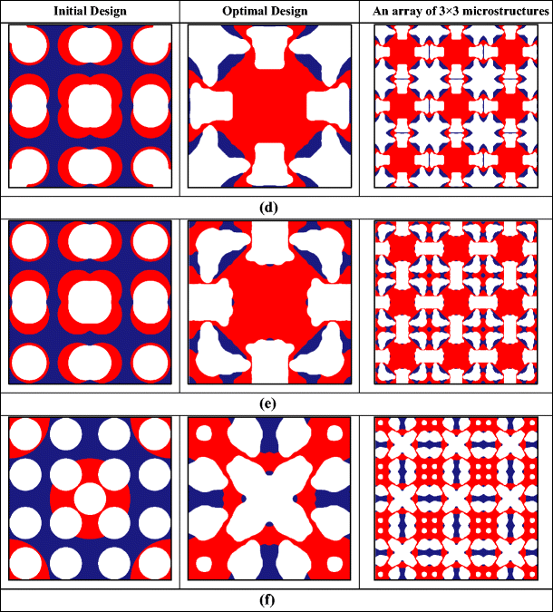

  

  Optimal microstructures for zero effective thermal expansion with different initial designs ((d), (e), and (f) are corresponding to the design case (d), (e) and (f) shown in Table 2)

  Table 2 Thermoelastic parameters for optimal microstructures

• Materials with negative effective thermal strain coefficients

  To obtain the materials with negative effective thermal strain coefficients, the optimization problem is conducted under different initial guesses and volume ratios. The horizontal, vertical and diagonal symmetry are applied to the microstructure. The optimal solutions for the two cases are shown in Fig. 14, and the corresponding parameters are given in Table 3.

  Fig. 14

  

  Optimal microstructures for negative effective thermal expansion with different initial designs ((g) and (h), are corresponding to the design case (g) and (h) shown in Table 3)

  Table 3 Thermoelastic parameters for optimal microstructures

  Beside the common features of the level set methods, it can be seen that similar optimized topologies are achieved due to dependency of final topology to initial design. Even though the MMA with a strong ability for searching a global optimal solution is employed as the optimizer, the dependency of initial designs is mainly caused by the non-convexity of optimization problem with the homogenized material. However, under the different objectives, obvious different detailed boundary shapes can be found in these two optimal designs. To achieve higher thermal expansion coefficient, thinner bars and hinge-like structures are generated in Case (g) to enhance larger deformation of the cellular structure when heated.

  The actual mechanisms behind the negative thermal expansion coefficients of the composite materials are very complex. From optimized topologies of the microstructure, we may find that the different material parts of the microstructure inside the design domain may become contact, due to the temperature increase of the microstructure. When a low bulk modulus is allowable, the main mechanism behind the negative thermal expansion phenomenon is the re-entrant cell structure having multi-material components, which will cause relatively large deformation when heated. The multi-material interfaces of the structure may bend and make the cell contract, similar to the behavior of the negative Poisson’s ratio materials (Lakes 1987; Milton 1992; Evans and Alderson 2000).

  From the above numerical examples, it can be found that the effective elastic and thermal expansion coefficients of the microstructure are dependent on both the internal structure (e.g. shapes and topologies) of the base cell and the way of deformation when loaded. Thus, in order to design a composite material with extreme properties, the microstructure will be prone to generate structures functionally similar to rotating rigid mechanisms (Wang et al. 2014). However, the topological shape optimization is a computational design mainly for structures, and it is difficult to generate the large rotating deformation like rigid-link mechanisms. This may be used to explain a phenomenon during the optimization process: the generation of re-entrant type structure that may be necessary for achieving the extreme thermoelastic property. The rotating effect of the design will make the microstructure have hinge-type connections locally inside the design domain. Since the microstructure is required to maintain the lower limit of bulk modulus, from the point of view of continuum structures, it is difficult to use structural shape and topology optimization method to generate microstructures that can exactly reach the extreme bounds of the material properties. However, the topology optimization is a powerful computational design tool, which can systematically generate new and novel microstructures for composites to achieve various desired and extreme properties.

5 Conclusions

We have developed a multi-phase topological shape optimization method for designing metamaterials with unusual properties using the numerical homogenization method and a level set method, in a way that is more efficient and effective. In this approach, the homogenization method is used to calculate the effective material properties of the microstructure, while MPLSM is established to achieve topological shape evolutions of the microstructure in the multi-material design domain. The proposed method is as a matter of fact a general computational design methodology, which is applicable to create any artificially structured composite metamaterials under periodicity. Our ongoing research is to extend the proposed topological shape optimization method to design problems of photonic metamaterials.

References

Allaire G, Jouve F, Toader A-M (2004) Structural optimization using sensitivity analysis and a level-set method. J Comput Phys 194(1):363–393
Allaire G, Dapogny C, Delgado G, Michailidis G (2014) Multi-phase structural optimization via a level set method. ESAIM Contr Optim Calc Var 20:576–611
Andreassen E, Andreasen CS (2014) How to determine composite material properties using numerical homogenization. Comput Mater Sci 83:488–495
Belytschko T, Xiao SP, Parimi C (2003) Topology optimization with implicit functions and regularization. Int J Numer Methods Eng 57(8):1177–1196
Bendsøe MP, Kikuchi N (1988) Generating optimal topologies in structural design using a homogenization method. Comput Methods Appl Mech Eng 71(2):197–224
Bendsøe MP, Sigmund O (1999) Material interpolation schemes in topology optimization. Arch Appl Mech 69(9–10):635–654
Bendsøe MP, Sigmund O (2003) Topology optimization: theory, methods and applications. Springer
Chen H, Chan C (2007) Acoustic cloaking in three dimensions using acoustic metamaterials. Appl Phys Lett 91(18):183518
Diaz AR, Sigmund O (2010) A topology optimization method for design of negative permeability metamaterials. Struct Multidiscip Optim 41(2):163–177
Dijk NP, Langelaar M, Keulen F (2012) Explicit level-set-based topology optimization using an exact Heaviside function and consistent sensitivity analysis. Int J Numer Methods Eng 91(1):67–97
Dijk NP et al (2013) Level-set methods for structural topology optimization: a review. Struct Multidiscip Optim 48(3):437–472
Dunning PD, Kim HA (2013) A new hole insertion method for level set based structural topology optimization. Int J Numer Methods Eng 93(1):118–134
Evans KE, Alderson A (2000) Auxetic materials: functional materials and structures from lateral thinking. Adv Mater 12(9):617–628
Gao T, Zhang W (2011) A mass constraint formulation for structural topology optimization with multiphase materials. Int J Numer Methods Eng 88(8):774–796
Gibiansky LV, Sigmund O (2000) Multiphase composites with extremal bulk modulus. J Mech Phys Solids 48(3):461–498
Guedes JM, Kikuchi N (1990) Preprocessing and postprocessing for materials based on the homogenization method with adaptive finite element methods. Comput Methods Appl Mech Eng 83(2):143–198
Guest JK, Prévost JH (2007) Design of maximum permeability material structures. Comput Methods Appl Mech Eng 196(4):1006–1017
Guest JK, Prévost JH, Belytschko T (2004) Achieving minimum length scale in topology optimization using nodal design variables and projection functions. Int J Numer Methods Eng 61(2):238–254
Huang X et al (2013) Topology optimization of microstructures of cellular materials and composites for macrostructures. Comput Mater Sci 67:397–407
Kang Z, Wang Y (2011) Structural topology optimization based on non-local Shepard interpolation of density field. Comput Methods Appl Mech Eng 200(49):3515–3525
Lakes R (1987) Foam structures with a negative Poisson’s ratio. Science 235(4792):1038–1040
Larsen UD, Sigmund O, Bouwstra S (1997) Design and fabrication of compliant micromechanisms and structures with negative Poisson’s ratio. J Microelectromech Syst 6(2):99–106
Li H, Li PG, Gao L, Zhang L, Wu T (2015) A level set method for topological shape optimization of 3D structures with extrusion constraints. Comput Methods Appl Mech Eng 283:615–635
Lu L et al (2013) Topology optimization of an acoustic metamaterial with negative bulk modulus using local resonance. Finite Elem Anal Des 72:1–12
Luo Z et al (2007) Shape and topology optimization of compliant mechanisms using a parameterization level set method. J Comput Phys 227(1):680–705
Luo J, Luo Z, Chen L, Tong L, Wang MY (2008a) A semi-implicit level set method for structural shape and topology optimization. J Comput Phys 227(11):5561–5581
Luo Z, Wang MY, Wang S, Wei P (2008b) A level set-based parameterization method for structural shape and topology optimization. Int J Numer Methods Eng 76(1):1–26
Luo Z, Tong L, Wei P, Wang MY (2009) Design of piezoelectric actuators using a multiphase level set method of piecewise constants. J Comput Phys 228(7):2643–2659
Luo Z, Gao W, Song C (2010) Design of multi-phase piezoelectric actuators. J Intell Mater Syst Struct 1045389X10389345
Luo Z, Zhang N, Gao W, Ma H (2012) Structural shape and topology optimization using a meshless Galerkin level set method. Int J Numer Methods Eng 90(3):369–389
Luo Z et al (2013) Topology optimization of structures using meshless density variable approximants. Int J Numer Methods Eng 93(4):443–464
Makhija D, Maute K (2013) Numerical instabilities in level set topology optimization with the extended finite element method. Struct Multidiscip Optim 1–13
Milton GW (1992) Composite materials with Poisson’s ratios close to −1. J Mech Phys Solids 40(5):1105–1137
Osher S, Fedkiw R (2002) Level set methods and dynamic implicit surfaces. Springer, New York
Otomori M et al (2012) A topology optimization method based on the level set method for the design of negative permeability dielectric metamaterials. Comput Methods Appl Mech Eng 237:192–211
Paulino GH, Silva ECN, Le CH (2009) Optimal design of periodic functionally graded composites with prescribed properties. Struct Multidiscip Optim 38(5):469–489
Sethian JA (1999) Level set methods and fast marching methods: evolving interfaces in computational geometry, fluid mechanics, computer vision, and materials science, vol 3. Cambridge university press
Sethian JA, Wiegmann A (2000) Structural boundary design via level set and immersed interface methods. J Comput Phys 163(2):489–528
Sigmund O (1994) Materials with prescribed constitutive parameters: an inverse homogenization problem. Int J Solids Struct 31(17):2313–2329
Sigmund O (2000) A new class of extremal composites. J Mech Phys Solids 48(2):397–428
Sigmund O (2001) Design of multiphysics actuators using topology optimization-Part I: one-material structures. Comput Methods Appl Mech Eng 190(49):6577–6604
Sigmund O, Torquato S (1996) Composites with extremal thermal expansion coefficients. Appl Phys Lett 69(21):3203–3205
Sigmund O, Torquato S (1997) Design of materials with extreme thermal expansion using a three-phase topology optimization method. J Mech Phys Solids 45(6):1037–1067
Sihvola A (2007) Metamaterials in electromagnetics. Metamaterials 1(1):2–11
Smith D, Pendry J, Wiltshire M (2004) Metamaterials and negative refractive index. Science 305(5685):788–792
Svanberg K (2005) The method of moving asymptotes—a new method for structural optimization. Int J Numer Methods Eng 24(2):359–373
Tavakoli R (2014) Multimaterial topology optimization by volume constrained Allen-Cahn system and regularized projected steepest descent method. Comput Methods Appl Mech Eng 276:534–565
Tavakoli R, Mohseni SM (2014) Alternating active-phase algorithm for multimaterial topology optimization problems: a 115-line MATLAB implementation. Struct Multidiscip Optim 49(4):621–642
Wang MY, Wang X (2004) “Color” level sets: a multi-phase method for structural topology optimization with multiple materials. Comput Methods Appl Mech Eng 193(6):469–496
Wang MY, Wang X, Guo D (2003) A level set method for structural topology optimization. Comput Methods Appl Mech Eng 192(1):227–246
Wang YQ et al (2014) Topological shape optimization of microstructural metamaterials using a level set method. Comput Mater Sci 87:178–186
Wang YQ et al (2015) A multi-material level set-based topology and shape optimization method. Comput Methods Appl Mech Eng 283:1570–1586
Wang Y, Gao J, Luo Z, Brown T, Zhang N (2016) Level set topology optimization for multimaterial and multifunctional mechanical metamaterials. Engineering Optimization. doi:10.1080/0305215x.2016.1164853, online
Wendland H (2006) Computational aspects of radial basis function approximation. Stud Computat Math 12:231–256
Xia Q, Wang MY, Wang S, Chen S (2006) Semi-Lagrange method for level-set-based structural topology and shape optimization. Struct Multidiscip Optim 31(6):419–429
Xie YM, Steven GP (1993) A simple evolutionary procedure for structural optimization. Comput Struct 49(5):885–896
Xie YM et al (2014) Designing orthotropic materials for negative or zero compressibility. Int J Solids Struct 51(23):4038–4051
Yamasaki S et al (2010) A structural optimization method based on the level set method using a new geometry-based re-initialization scheme. Int J Numer Methods Eng 83(12):1580–1624
Zhou M, Rozvany GIN (1991) The COC algorithm, Part II: topological, geometrical and generalized shape optimization. Comput Methods Appl Mech Eng 89(1):309–336
Zhou S, Wang MY (2007) Multimaterial structural topology optimization with a generalized Cahn–Hilliard model of multiphase transition. Struct Multidiscip Optim 33(2):89–111
Zhou M, Wang MY (2012) A semi-lagrangian level set method for structural optimization. Struct Multidiscip Optim 46(4):487–501
Zhou S et al (2011) Topology optimization for negative permeability metamaterials using level-set algorithm. Acta Mater 59(7):2624–2636
Acknowledgements
This research is supported in part by Australian Research Council - Discovery Project (DP160102491, DP150102751), the National Natural-Science-Foundation of China (51575204), and the Science and Technology Support Program of Hubei Province of China (2015BHE026), as well as by the Open Research Foundation (DMETKF2015010) of State Key Lab. of Digital Manufacturing Equipment & Technology, Huazhong University of Science & Technology, Wuhan, China.
Author information
Authors and Affiliations
Corresponding author
Rights and permissions
About this article
Cite this article
Wang, Y., Luo, Z., Zhang, N. et al. Topological design for mechanical metamaterials using a multiphase level set method. Struct Multidisc Optim 54, 937–952 (2016). https://doi.org/10.1007/s00158-016-1458-6
Received:
Revised:
Accepted:
Published:
Issue Date:
DOI: https://doi.org/10.1007/s00158-016-1458-6