Auditory Systems

Abstract

Sound waves are the adequate physical stimulus for hearing organs of vertebrates and insects. Sound waves may originate from abiotic events, for example, from running water, breaking waves at beaches, movement of bushes and trees in the wind, howling storms, or thunder. Most interesting for animals, however, are sounds generated by other moving animals – rustling noises may signal the presence of prey or predator – or by special sound-producing organs of insects and vertebrates which use sounds in communication. The morphology of hearing organs is adapted to the physical properties of the sounds to be perceived. Central to all hearing organs are mechanoreceptors (see Chap. 16). In the present chapter, we deal with mechanoreceptors serving in hearing organs as the sensitive elements through which sound-induced motion is translated into activation of the central auditory systems of animals, thus providing information about the presence of sound waves in surrounding water or air. Sound waves traveling in and being picked up from solids are not considered here (see Chap. 16).

These keywords were added by machine and not by the authors. This process is experimental and the keywords may be updated as the learning algorithm improves.

Sound waves are the adequate physical stimulus for hearing organs of vertebrates and insects. Sound waves may originate from abiotic events, for example, from running water, breaking waves at beaches, movement of bushes and trees in the wind, howling storms, or thunder. Most interesting for animals, however, are sounds generated by other moving animals – rustling noises may signal the presence of prey or predator – or by special sound-producing organs of insects and vertebrates which use sounds in communication. The morphology of hearing organs is adapted to the physical properties of the sounds to be perceived. Central to all hearing organs are mechanoreceptors (see Chap. 16). In the present chapter, we deal with mechanoreceptors serving in hearing organs as the sensitive elements through which sound-induced motion is translated into activation of the central auditory systems of animals, thus providing information about the presence of sound waves in surrounding water or air. Sound waves traveling in and being picked up from solids are not considered here (see Chap. 16).

We will see that hearing organs of vertebrates are rather homogeneous in morphology and function because hearing via the natural routes is always ­coupled with functions of the inner ear. In contrast, hearing organs of insects are morphologically diverse and located at various places of the body indicating different evolutionary roots. In any case, it must be emphasized that the presence and activation of hearing organs is not sufficient for sensing sounds, not even necessary in the case of electrical stimulation of the central auditory system via modern hearing aids. It is the processing in the central nervous system that leads to the perception of sounds. Vertebrates (humans included) “hear” with their brains.

Several examples will show that sound perception can happen at different levels of complexity of neural processing. Reflexes such as the startle response to a loud sound or the orienting response to a soft sound are at the base level of processing. Instinctive responses to sounds require motivation to respond and often discrimination of the acoustic quality of sounds. Acoustic quality refers to many parameters such as intensity, spectral content, and temporal structure of a sound, and to the audibility of a sound in masking background noise, i.e., to the signal-to-noise ratio. Instinctive responses occur, for example, in sound communication, predator avoidance, and predator location of insects. Finally, sound recognition requires learning of sound patterns in order to use certain sounds for orientation and/or communication. This happens in many birds and mammals. Necessary for pattern recognition is again the ability to discriminate the acoustic qualities of sounds which is, besides sound source localization, the main purpose of auditory systems.

17.1 The Physics of the Stimulus

Oscillating bodies and membranes (e.g., vocal chords, air bladders, elytra, membranes of loudspeakers) are the sources of sound waves when they push and pull attached air or water molecules, and the oscillation of these molecules spreads out in the medium. The ­movement of the molecules back and forth in the axis of the direction of the propagation of the sound wave creates local compressions and dilutions of the molecules. The distances between these compressions or dilutions along the axis of sound propagation equal the wavelength (λ) of the sound, the rate of oscillations per second (Hz) expresses the frequency (f) of a tone. The product of f and λ is the velocity c of the sound wave (c  =  f λ [m/s]) which amounts to about 330 m/s in air (at sea level) and to about 1,500 m/s in water. This means that tones of a given frequency have about five times the wavelength in water compared to propagating in air. Sounds in water travel much longer distances before they are attenuated below the hearing threshold. For example, whales can hear songs of other whales over many hundreds of kilometers depending on the noise conditions in the sea.

Taking young humans as reference, frequencies are classified as belonging to the audible range (20–20,000 Hz), to infrasound (f  <  20 Hz), or ultrasound (f  >  20,000 Hz). Because of the high frequencies of oscillations (short wavelengths) ultrasounds lose energy very rapidly when traveling through air. Thus, ultrasound can be used only for short-range orientation (e.g., echolocating bats) or communication (e.g., social calls of bats and rodents). Infrasound, however, can travel hundreds of kilometers with little attenuation so that animals can use infrasound for long-distance communication (e.g., elephants) or for locating sources of infrasound (breaking waves at beaches, wind blowing through mountain valleys, thunderstorms) for navigation (e.g., pigeons).

The pressure difference between the compression and dilution maxima of molecules in propagating sounds equals the sound pressure amplitude (p _A) expressed in Pascals (Pa  =  N/m²). Microphones measure the sound pressure (p) which is the effective sound pressure amplitude (p  =  0.5 p _A/)). The working ranges of most of the hearing organs of animals comprise many orders of magnitude between the lowest just perceptible pressure (p at the absolute hearing threshold) and the highest pressure beyond which the hearing organs are irreversibly damaged, in humans 10¹³ in sound intensity (I [Watt/m²]) or 3.2  ×  10⁶ in sound pressure (I  ∼  p ²). These extraordinarily large ranges and the logarithmic translation of sound pressure or intensity into perception (see Fechner’s rule, Chap. 12) led to the introduction of the sound pressure level (SPL), a dimensionless quantity which is expressed in units of Decibels (dB). For measurements in air the SPL  =  20 log p/p ₀ [dB] with p ₀  =  20 μPa (reference sound pressure at the average human hearing threshold at 1 kHz frequency). These definitions adjust the working range of the human ear from 0 to 130 dB at 1 kHz frequency. At 0 dB SPL, the movement amplitude of air molecules is in the order of 10^–12 m which is about 100 times less than the diameter of a hydrogen atom. Animals like cats being even more sensitive than humans, may reach −18 dB at their absolute hearing threshold [9]. This incredible sensitivity to sound pressure from movement amplitudes of molecules is the maximum to be biologically meaningful because the thermal noise in air masks the perception of even fainter sounds.

Sound pressure is the sound parameter appropriate for stimulating animals having tympanic membranes (eardrums) or comparable structures such as air bladders. The velocity of the molecules or particle movements in sound waves is the appropriate stimulus for animals having antennae or hair sensilla on their body (insects) or hair cells with a long kinocilium, often covered by membranes or otoliths in organs of their inner ear (vertebrates). Literature about the physics of sounds can be found in many general textbooks about sound and hearing (e.g., [3, 30, 48]).

17.2 Mammals

17.2.1 Peripheral Auditory System

Peripheral auditory systems of mammals (Fig. 17.1) divide into three parts, (i) the outer ear and the middle ear capturing sound to transfer it to the inner ear, (ii) the cochlea which houses the sound sensitive epithelia of the inner ear, and (iii) the auditory nerve transmitting the encoded sound information from the cochlea to the brain.

Fig. 17.1

The human ear as an example of a mammalian ear with outer ear (pinna and concha, ear canal, tympanum  =  eardrum), middle ear with the three ossicles, and the inner ear with the cochlea as the actual hearing organ

17.2.1.1 Outer Ear, Middle Ear

Most mammals are land vertebrates, and so for them sound in air has to be transferred into the fluid spaces of the cochlea. Since the impedance of air against the propagation of sound waves is about 3,600 times smaller than the impedance of water, about 99 % of the sound energy would be reflected at the entrance to the cochlea without special structures of the outer and middle ear amplifying the sound pressure and, thus, matching the impedances of the media [3, 21]. The outer ear and the middle ear provide two steps of sound frequency-dependent pressure amplification. The outer ear includes an outstanding, often movable part, the pinna, a folded cartilaginous part, the concha, and the external ear canal, the meatus, ending at the eardrum (tympanic membrane). By resonances and filtering, this construction selectively amplifies certain sound frequencies, about 2–4 and 11–13 kHz in human adults (Fig. 17.2) [3, 37], thus improving the auditory sensitivity at these frequencies up to about 20 dB depending on the angle of incidence of the sound in the horizontal plane (azimuth angle, Fig. 17.2). The spectral shape of the amplification depends also on the vertical angle of incidence of the sound providing cues for the estimation of the elevation of the sound source relative to the ear. Human babies and young mammals learn to use the direction-dependent frequency transfer function of their outer ears in order to locate sound sources in ­azimuth and elevation and to discriminate between front and back locations.

Fig. 17.2

Transfer functions of the human outer ear. The relative increase of the sound pressure level at the eardrum relative to outside the ear is shown for tones arriving at the ear from several horizontal directions (angles of incidence). Angle- and frequency-dependent amplification up to about 20 dB is evident (Modified from Buser and Imbert [3] with permission)

The cavities of the middle ear and the mouth are connected with the Eustachian tube through which static pressures between the cavities can be equalized. A chain of three bones, the middle ear ossicles – ­malleus (hammer), incus (anvil), and stapes (stirrup) – connects the eardrum with the membrane overlying the oval window which is the entrance to the fluid spaces of the inner ear (Fig. 17.1). This middle ear construction serves as a sound pressure amplifier via three mechanisms (Fig. 17.3a; [3, 21, 37]):

Fig. 17.3

(a) Functional principle of sound transmission through the mammalian middle ear. The sound pressure at the stapes footplate (p _S) is amplified relative to the sound pressure at the tympanic membrane (p _T) by (1) the area ratio A _T : A _S, (2) the ratio of the lever arms of malleus and incus (l _M : l _I), and (3) by the flexure of the area of the tympanic membrane (A _T). (b) Comparison of the cat audiogram with its middle ear transfer function. This function (1/amplitude of stapes movement) is plotted on an arbitrary scale. The larger the amplitude is, the better is the sound transfer and the more sensitive is the ear. In the corrected transfer function, the highpass filter of the helicotrema at the cochlear apex is considered. The shape of the audiogram is very similar to the shape of the corrected middle ear transfer function (Compare Buser and Imbert [3] and Pickles [30])

• 1. The area of the tympanic membrane (A _T) is always larger than the area of the stapes footplate (A _S) providing amplification according to the area ratio (A _T/A _S) which in humans amounts to 0.55 cm²/0.032 cm²  ≈  17.

• 2. The ossicles function as a lever system with the lever arm of the malleus (l _M) being always larger than the lever arm of the incus (l _I). In humans the level ratio (l _M/l _I) is about 1.3.

• 3. The malleus attaches asymmetrically at the tympanic membrane which provides another lever amplifying the sound pressure by a factor of 1.4 in humans.

The whole amplification of the pressure at the stapes footplate (p _S) from the pressure at the tympanic membrane (p _T) is equal to the product of all three factors which for humans amounts to p _S  =  p _T  ×  17  ×  1.3  ×  1.4  =  31 p _T. Other mammals have amplification factors between about 10 and 90 leading to pressure gains between about 20 and 39 dB. The largest pressure gain of 39 dB is known from the cat providing this mammal with the most sensitive ear of all animals tested so far.

In the frequency domain, the middle ear response is that of a bandpass filter with a broad, species-specific passing range and more or less steep slopes of attenuation at the low- and high-frequency sides (Fig. 17.3b) [37]. The cutoff frequency at the low-­frequency side is determined mainly by the mechanical properties and sizes of the eardrum and the oval window. The larger the eardrum and the more elastic the stapes is coupled to the oval window, the more effectively can these membranes follow the long wavelengths of low-frequency sounds. Thus, elephants with their large eardrums can hear infrasound down to about 10 Hz. The cutoff frequency at the high-frequency side is determined mainly by the inertia of the ossicles and energy losses by friction in and bending of the ossicular chain. Small (light) and stiff ossicles such as those of bats and rodents favor transmission of ultrasounds.

Two muscles, the tensor tympani attached to the malleus, and the stapedius muscle influence the sound transmission through the mammalian middle ear. A reflexive contraction of the muscles (middle ear reflex) to loud sounds increases the stiffness of the middle ear and attenuates the passage of sounds, ­especially those of low frequencies (in humans below about 2 kHz). The effect is (i) a protection of the inner ear against damage by loud sounds except when the sound onset is instantaneous as in gun shots, (ii) a damping of self-produced sounds transmitted by bone conduction to the middle ear so that listening to others is less disturbed by simultaneously produced own sounds, and (iii) an attenuation of low-frequency sounds that can mask the perception of higher frequencies in the inner ear important for the discrimination of communication sounds [3, 37].

In summary, the outer and middle ears of mammals largely determine the shape of their species-specific frequency response curves and the absolute sensitivity for hearing tones, both expressed in the absolute auditory threshold curve, the audiogram. In Fig. 17.4, audiograms for 60 terrestrial mammalian species are shown, all measured in behavioral hearing tests [9]. It is evident that humans are rather non-specialized ­low-frequency listeners.

Fig. 17.4

Audiograms of 64 mammalian species obtained from behavioral tests. The human audiogram is shown in red. The average audiogram for birds (blue) and the average high-­frequency parts of the amphibian (green) and fish (orange) audiograms are also shown for comparison (Modified from Fay [9] with permission). On average, high-frequency hearing is improved and extended by about six octaves during vertebrate evolution from fish to mammals

17.2.1.2 Cochlea

Fluid spaces and membranes. The cochlea (Fig. 17.1) equals an elongated and coiled basilar papilla of the inner ear of birds and reptiles [3, 22, 30]. It consists of three main fluid spaces and several membranes (Fig. 17.5).The scala vestibuli, starting at the oval window and running up to the helicotrema at the apex of the cochlea, and the scala tympani, running from the helicotrema to the round window, are filled with Na⁺-rich perilymph, resembling extracellular fluids. The scala media is separated from the scala vestibuli by the Reissner membrane and from the scala tympani by the basilar membrane. It contains intracellular-like K⁺-rich endolymph which is provided by the stria vascularis at the lateral cochlear wall. The actual hearing organ is the organ of Corti, sitting on the basilar membrane in the scala media (Fig. 17.5). The organ of Corti is covered with the tectorial membrane. The tips of the longest stereocilia of the outer hair cells are inserted in the tectorial membrane, the tips of the stereocilia of the inner hair cells are only loosely attached.

Fig. 17.5

Radial section through the scala media of the mammalian cochlea. Reissner’s membrane separates the scala media from the scala vestibuli. The organ of Corti with the hair cells and supporting cells sits on the basilar membrane which separates the scala media from the scala tympani. The afferent and efferent innervation of an inner and an outer hair cell is enlarged. AF afferent nerve fibers, EF efferent nerve fibers (Modified from Smith [42] with permission)

Basilar membrane displacement and tonotopy. A movement of the stapes in response to, for example, the sine wave of a tone leads to a push-and-pull movement of the perilymph in the scala vestibuli inducing the same movement to the very flexible Reissner membrane and the endolymph of the scala media, i.e., a movement towards and away of the basilar membrane. The basilar membrane is stiff (thick and narrow) at the base and flexible (thin and wide) at the apex of the cochlea. Therefore, it will move at the base only in response to high-frequency (high-energy) moves of the endolymph. According to the stiffness gradient of the basilar membrane, fluid movements induced by tones of different frequencies will induce movements of the basilar membrane the farther at the apex the lower the frequencies are. Thus, sounds with a complex frequency spectrum such as vowels of human speech, induce waves of fluid movements that travel along the basilar membrane (traveling waves; [29, 34]) up to those locations of stiffness allowing a maximum displacement of the membrane to matching ­frequencies in the sound (Fig. 17.6a, b). At the ­displacement maximum, there is a maximum ­movement of the fluid in the scala tympani towards the flexible round window, which moves towards the middle ear cavity where the energy from the initial stapes movement is lost. This loss of energy leads to the rapid ­collapse of a traveling wave just after the displacement maximum of the basilar membrane has been reached.

Fig. 17.6

(a) Instantaneous picture of the deflection of the mammalian basilar membrane by a travelling wave initiated by a pure tone. (b) Travelling waves and their envelopes due to a high, medium, and low frequency tone. (c) Rectified envelope of a travelling wave in response to a medium tone frequency at three sound pressure levels. Loud tones lead to an overproportional extension of the basilar membrane deflection towards the cochlear base

The stiffness gradient along the basilar membrane is the origin of the cochlear tonotopy, giving each sound frequency a different place of maximum stimulation of the cochlear hair cells (Fig. 17.6). In mammals with a continuous stiffness gradient of the basilar membrane, this frequency-to-place transformation follows the function f  =  A (10^ax – k) with f  =  tone frequency; x  =  location of maximum displacement on the basilar membrane as distance from the apex; A, a, k  =  species-specific values whereby k can be set to 1 in most cases. In humans the values are A  =  165.4, a  =  0.06, k  =  1. Although very different in length from about 6 mm in some mice to more than 60 mm in whales, the cochleas of most mammals are scale models of each other [12]. Some mammals, however, such as horseshoe bats and the mustache bat, have a discontinuous stiffness ­gradient of the basilar membrane. The tonotopy does not follow the smooth frequency gradient according to the general equation above, but shows an auditory fovea, i.e., spreading of a small frequency range represented near the discontinuity over a long cochlear ­distance [31].

With increasing sound level of a tone, the range of displacement of the basilar membrane increases asymmetrically around its maximum with a much larger involvement of basal parts when sounds are loud (Fig. 17.6c; [34]). The physiological effect is that loud sounds of any frequency stimulate the hair cells in the high-frequency range of the tonotopy so that these hair cells suffer more from a continuous stimulation in a loud environment than hair cells near the cochlear apex. The consequence is damage of hair cells near the cochlear base with increasing age causing the high-frequency hearing loss of many senior people.

Hair cells – mechanoelectrical transduction [1, 29]. There are two populations of secondary sensory cells (without own axon) in the mammalian organ of Corti, the inner hair cells (IHCs) in one row (about 4,000 in humans), and the outer hair cells (OHCs) in three to five rows (together about 12,000 in humans) along the cochlea (Figs. 17.5 and 17.7). The apical membrane of the hair cells has 50–100 elongated microvilli, the actin-containing stereocilia are about 2–5 μm long.

Fig. 17.7

Scheme of the innervation pattern of inner and outer hair cells in the mammalian cochlea. AF afferent fibers, EF efferent fibers, HP habenula perforata (the holes in the bone, where the fibers enter the organ of Corti; see Fig. 17.5) (Modified from Spoendlin [43] with permission)

The outer hair cells regulate the sensitivity of the IHCs to the shearing motions of the tectorial membrane when the basilar membrane moves up and down. Upward movements cause deflection of stereocilia towards the tallest ones, a relative sliding between adjacent pairs of stereocilia, tension of the tiplinks (catherin/protocadherin protein threads) between the stereocilia, and, by that, mechanical opening of ion channels for cations (compare Fig. 16.3, Chap. 16). A gradient of about 150 mV of electrical potential between scala media (+80 mV) and the interior (−70 mV) of the OHCs leads to an influx mainly of K⁺ from the K⁺-rich scala media into the cells and, thus, to pulses of depolarization of the OHCs in the rhythm of the stereocilia movement (mechanoelectrical transduction). The depolarization pulses shorten the OHCs, repolarization and hyperpolarization lengthen them. This electromotility is based on the protein ‘prestin’ densely packed along the lateral walls of the OHCs (see Chap. 16). Since the OHCs are coupled with the tectorial membrane via their stereocilia, and are part of the organ of Corti which is attached to the basilar membrane, the electromotility of the OHCs amplifies the displacement amplitude of the basilar membrane and changes the width of the fluid-filled space between the upper hair cell surface and the tectorial membrane: shortening of the OHCs pulls the tectorial membrane closer to the hair cell surface. This affects also the IHCs because their stereocilia get in closer contact with the tectorial membrane and/or are more susceptible to the fluid motions between hair cell surface and tectorial membrane. The net effect is an increase in IHC sensitivity to basilar membrane motion in the order to 40–60 dB. This boosting of IHC sensitivity by OHC action becomes most evident when mammals with increasing age suffer from a considerable hearing loss in the high-frequency range due to progressive loss of OHCs from the basal end of the cochlea.

The OHC motility is also origin of the amazing phenomenon of ‘otoacoustic emissions’, which are tones produced in the cochlea. Spontaneous local OHC movements induce traveling waves of the basilar membrane feeding back to the middle and outer ear. Thus, otoacoustic emissions occur as displacements of the cochlear round and oval windows or of the tympanum or even as tones in the ear canal. Measurements of the presence and amplitude of otoacoustic emissions are, therefore, an important noninvasive diagnostic tool for assessing functional OHCs in the cochlea [29]. Otoacoustic emissions and amplification also occur in non-mammalian ears that lack OHCs. In these animals, amplification arises from active hair bundle motions that are powered by the transduction apparatus [22, 34].

Inner hair cells have the same mechanoelectrical transduction through the deflection of the stereocilia as the OHCs. However, IHCs are not motile so that the depolarization by K⁺ influx has only chemical and electrical consequences in the cells.

Hair cells – electrical potentials, synapses, and innervation [3, 22, 30, 43]. The mechanoelectrical transduction mainly of the OHCs leads to an alternating potential called cochlear microphonic potential which is a receptor potential that closely reproduces the waveform of the sound input. Synchronous cochlear microphonics from many hair cells can be recorded with electrodes outside the cochlea even from the scalp. Another type of receptor potential of the hair cells is the summating potential reflecting a slow depolarization of the resting potential due to ­cation influx that is not immediately compensated by a respective cation efflux. The receptor potentials cause a Ca²⁺ influx leading to the release of the ­neurotransmitter glutamate from synaptic vesicles (see Chap. 16). The presynaptically released glutamate binds mainly to postsynaptic AMPA receptors to open Na⁺ channels for ultimately generating action potentials in the bipolar cells of the cochlear spiral ganglion. The axons of the spiral ganglion cells join together as cochlear nerve fibers in the auditory nerve and run to the first auditory center of the brain, the cochlear nucleus.

The IHCs are innervated by at least 90 % of the afferent cochlear nerve fibers (about 60,000 in humans). Mostly, one afferent fiber contacts only one IHC, and one IHC is innervated by 10–30 fibers (divergent innervation pattern; Fig. 17.7). Thus, almost all auditory information is sent to the brain via the IHCs. They provide the necessary and sufficient cochlear output via the cochlear nerve fibers for many perceptual abilities including sound localization and pattern analysis and discrimination. The function of the few afferent fibers from the OHCs is not known.

OHCs, especially those responding best to low- and mid-frequencies of a species’ hearing range, may receive strong innervation by efferent auditory nerve fibers sending information from auditory brain centers back to the cochlea (Figs. 17.5, 17.7, and 17.11). Efferent activity hyperpolarizes OHCs causing reduction of the depolarization by K⁺ influx through the deflected stereocilia. Thus, the electromotility and the amplification effect of the OHCs on the mechanical stimulation of the IHCs are reduced. Ultimately, efferent activity reduces the cochlear sensitivity to tones by about 10–20 dB. Since efferent activity can be focused on small clusters of OHCs representing a certain frequency of the cochlear tonotopy, the perception of frequency components in a sound important for communication can be enhanced by efferent suppression of processing unimportant but masking frequency components. By this mechanism of peripheral contrast enhancement, the listening brain can modulate its own perception according to the knowledge of what sound spectra are expected.

IHCs do not receive direct efferent innervation. Efferent fibers contact afferent fibers at or near their synapse with the IHCs (Figs. 17.5 and 17.7) suggesting a modulation of the afferent activity of auditory nerve fibers. This modulation may rather relate to long-term adjustments in sensitivity and temporal precision of coding sounds than to short-term control as is the case with the efferent fibers to the OHCs.

17.2.1.3 Coding of Sounds in the Auditory Nerve

The auditory nerve of vertebrates is that part of the VIIIth brain nerve which innervates the hearing organs in the inner ear, here the mammalian cochlea. The bipolar neurons of the cochlear spiral ganglion innervate the hair cells with the distal part of their axons and send the information with the proximal part to the cochlear nucleus (Figs. 17.5, 17.7, and 17.10).

Coding of sound frequency [3, 30]. There are two codes for sound frequencies in the auditory nerve fibers: the place code based on the cochlear tonotopy is functional for all frequencies that can stimulate the cochlea, the phase code based on time-locking of action potentials to the sound waveform is functional only up to about 4 kHz.

The afferent fibers from the hair cells code the local displacement pattern of the basilar membrane to traveling waves by the position of their innervation (Figs. 17.6 and 17.7). The frequency tuning of auditory nerve fibers expressed by the excitatory tuning curve (Fig. 17.8) is derived from the envelope function of the traveling wave (Fig. 17.6c). The excitatory tuning curve borders the frequency range (receptive field) within which the fiber discharges in response to tones above the spontaneous activity. Thus, the excitatory tuning curve describes the frequency-dependence of the neuronal response threshold. The lowest threshold is at the fibers characteristic frequency (CF) which equals the fibers best frequency (BF) where it responds with the highest rate at any sound level. The slopes of the excitatory tuning curve are flanked by areas of lateral suppression (Fig. 17.8). Tones in these areas partly or totally suppress the response of the fiber to tones in the receptive field. Different from lateral inhibition caused by neural interaction in the retina (see Chap. 18), lateral suppression in auditory nerve fibers is caused by mechanical nonlinearities in the cochlea which also give rise to the formation of distortion tones (e.g., 2f ₁ – f ₂ and f ₂ – f ₁; in both cases f ₂  >  f ₁) when two tones simultaneously stimulate the ear [29, 34].

Fig. 17.8

Examples of frequency tuning curves of auditory nerve fibers having a medium (left) or a high (right) characteristic frequency (CF). Areas of lateral suppression (LS) are indicated in red

The locking of action potentials in auditory nerve fibers to the phase of a low-frequency tone or the phase of amplitude modulation of a high-frequency tone or a frequency complex is a neural code for tone frequency or rate of amplitude modulation. The spike pattern is decoded in higher auditory brain centers and leads to the perception of pitch and to the ability to perceive and discriminate musical intervals. Because action potentials in auditory nerve fibers of mammals occur with a statistical variation of 165 μs, the phase code for frequency is limited to 1/165 μs  =  6 kHz in theory. The 0.5–1 ms duration of action potentials and their refractory period allow phase coding by a single fiber only up to about 800 Hz. Several fibers can cooperate, however, to code pitch and musical intervals in the time domain up to about 4 kHz by locking their spikes to different cycles of the sound stimulus so that every cycle is labeled by at least one spike (volley principle of coding).

Coding in the time domain. Auditory nerve fibers respond to sound onsets with a phasic discharge and continue to respond at a lower tonic level as long as the sound lasts (phasic-tonic response; Fig. 17.12). Thus, the onsets and durations of sounds in a series (e.g., syllables in human speech) are expressed in the temporal response patterns of the fibers. This coding of sound series or rhythms by onset responses is possible up to intersound intervals of 20–30 ms. If the intervals are shorter, i.e., the repetition rate of the sounds is higher than about 30–50 Hz, the sound series is coded as an amplitude-modulated sound with a given modulation frequency (see above) and is perceived as a continuous sound with a certain pitch.

Coding of sound intensity [3, 19, 30]. Auditory nerve fibers differ in their response properties depending on the place where they innervate a given inner hair cell. Fibers innervating at the side of the tunnel of Corti (Fig. 17.5) have high spontaneous activity, low response thresholds and small dynamic ranges (about 10–20 dB) of spike rate increase with increasing tone level (Fig. 17.9a, fiber 1). Fibers innervating at the side of the spiral limbus (Fig. 17.5) have low spontaneous activity, higher response thresholds, and larger dynamic ranges (about 30–70 dB; Fig. 17.9a, fiber 2). Thus, fibers of the same CF, coding for the same sound frequency, can cover together a threshold range of about 60 dB (Fig. 17.9b) and a dynamic range of about 70 dB. By adding the ranges of response threshold and rate increase, the fibers from a given cochlear location can encode a 130 dB range of sound intensity just via their total number of spikes. Therefore, it is assumed that the intensity of a tone perceived over the dynamic range of hearing, which is about 130 dB in the most sensitive frequency range of humans, is encoded at the level of the auditory nerve by the population of active nerve fibers, originating at the cochlear place of tone frequency representation, and their cumulated spike rate.

Fig. 17.9

(a) Two examples of rate-level functions of auditory nerve fibers. Fiber 1 has a high spontaneous activity (about 80 spikes/s), a low tone-response threshold (near 40 dB), and a small dynamic range (about 25 dB) of response rate (action potentials/s, AP/s) increase with increase of the sound pressure level. Fiber 2 has very low spontaneous activity, a higher threshold (almost 60 dB), and a larger dynamic range (about 40 dB). (b) Behavioral audiogram of the cat and absolute response thresholds (the thresholds at the CF) of cat auditory nerve fibers with high, medium, and low spontaneous activity (Sa) (From Liberman and Pickles [19, 30] with permission)

17.2.2 Central Auditory System

17.2.2.1 General Anatomy – Auditory Pathways

The central auditory system consists of ascending (afferent) and descending (efferent) projections with several centers of processing at each level of the brain (Figs. 17.10 and 17.11) [20, 38]. This parallel and ­hierarchical processing is unique among vertebrate sensory systems and certainly different from those of the visual and somatic sensory systems.

Fig. 17.10

Diagrams of the ascending (afferent) auditory pathways of an amphibian, bird, and mammal. The diagrams show the most important connections in only one half of the brain with origin in the left inner ear (cochlea). The main pathways cross to the other side, so that the projections starting in the left inner ear mainly end in the right-side midbrain and further in the right telencephalon. Heavy lines strong projections, thin lines weaker projections, sA several areas, sN several nuclei, N nucleus

Fig. 17.11

Diagram of the main descending (efferent) auditory pathways of a mammal starting at the left-side auditory cortex and ending finally in the right-side cochlea at the outer hair cells (HC) or at the afferent fibers from the inner HC. As for the ascending pathways (Fig. 17.10), the main efferent pathways cross to the other side below the midbrain level. sA several areas, sN several nuclei, N nucleus

Auditory nerve fibers enter the medulla oblongata and, in mammals, project to several cell types in the complex of the cochlear nucleus (Fig. 17.12; [35]). There, the rather homogenous phasic-tonic tone responses, the V-shaped frequency tuning curves, and sigmoid rate-level functions of auditory nerve fibers change to cell type-specific patterns (Fig. 17.12). These patterns are forwarded to different target nuclei in the ascending auditory system. Primary patterns reach the next level of processing, the nuclei of the superior olivary complex (medulla oblongata) where the inputs from both ears interact to extract the information for sound localization (see Sect. 17.2.2.5). Derived patterns occur as tone responses of purely phasic (onset) activity, or as choppers (phasic-tonic activity whereby the tonic part is chopped in bursts) or pausers (a short gap between a phasic and the following tonic activity). In addition, tuning curves with inhibitory side bands (caused by synaptic inhibition), and peaked rate-level functions (Fig. 17.12) are observed. Neurons with such derived tone response characteristics mainly provide excitatory input to the nuclei of the lateral lemniscus (pons of the metencephalon) and the inferior colliculus of the midbrain. Ascending output from the nuclei of the superior olivary complex (excitatory and inhibitory) and the nuclei of the lateral lemniscus (mainly inhibitory) also reaches the inferior colliculus. That is, ascending information from lower brainstem nuclei, mainly from the ­contralateral side (auditory chiasm; Fig. 17.10) converges in the main (central) nucleus of the inferior colliculus of each brain hemisphere. From there, both excitatory (glutamatergic) and inhibitory (GABAergic) neurons project to the nuclei of the medial geniculate body (thalamus of the diencephalon) from where auditory information is distributed to many brain areas. In mammals, primary targets are the auditory areas of the cerebral cortex (Figs. 17.10, 17.13, and 17.16a). Other targets are the nuclei of the striatum, the hippocampus (part of the pallium), and nuclei of the basal telencephalon such as the amygdala and the preoptic area. These projections provide direct auditory input to motor coordination, especially for vocalizations (striatum), to associative learning (pallium), and to the coordination of instincts (basal telencephalon, limbic system).

Fig. 17.12

Diagram of the divergent innervation of five different cell types in the cochlear nucleus by an auditory nerve fiber. The cell types are named (from above) fusiform, octopus, globular, multipolar, and spherical (bushy). The phasic-tonic (pht) temporal response of the auditory nerve fiber to a tone burst may change to different cell type-specific patterns such as pauser (p), phasic or “on” (ph), and chopper (ch) or remain unchanged (in the spherical cells). The rate-level functions of the cell types may have a sigmoid shape or show a peak (best level) at a certain level. The frequency tuning curves also differ in shape and may include inhibitory areas, i.e., sounds in these areas inhibit the response to sounds in the excitatory area bordered by the tuning curve. The axons of the cell types in the cochlear nucleus terminate in different areas of the auditory pathway: IC inferior colliculus, LL lateral lemniscus, TB trapezoid body of the superior olivary complex (SO), SOmi, SOmc, SOli medial superior olive ipsilaterally, or contralaterally, or lateral superior olive ipsilaterally (respectively) (Compare Romand and Avan [35] and Rouiller [38])

Fig. 17.13

Transformation of the cochlear tonotopy of the cat (a) to the tonotopic representations at various levels of the auditory pathway. The shown numbers (0.5, 1, 2, 5, 8, 10, 12, 20, 30) are tone frequencies in kHz representing the characteristic frequencies of neurons at the indicated places of the tonotopic map. (b) NCd nucleus cochlearis dorsalis, NCav, NCpv nucleus cochlearis anteroventralis and posteroventralis, SOl lateral superior olive, SOm medial superior olive. (c) Central nucleus of the inferior colliculus. (d) Nucleus ventralis lateralis and ovoidalis of the medial geniculate body. (e) The primary (AI), secondary (AII), and anterior (AAF) fields of the auditory cortex. (b) and (d) show a transverse, (c) a sagittal section, (e) is a lateral view on the neocortex. N nucleus, h high frequencies, l low frequencies (Compare Romand and Avan [35] and Rouiller [38])

Figure 17.10 shows clearly that the ascending auditory pathways in the brainstem form a system of parallel/hierarchical processing, indicating a division of labor between the auditory centers in the analysis of sound parameters which is followed by an integration of information in the inferior colliculus. The integrated information is then passed on to the medial geniculate body and the auditory cortex, which have strong reciprocal connections and serve as a unit to allow auditory learning and complex behavioral control through sounds.

Descending auditory pathways have been studied mainly in mammals. They start at the auditory cortex and end contralaterally (chiasm at the level of the brainstem) at the cochlear outer hair cells or at the afferent fibers from the inner hair cells (Fig. 17.11). They ­connect in a parallel and hierarchical way the same auditory centers as the ascending pathways. Thus, there are many functional loops operating by positive or negative feedback – depending on excitatory and/or inhibitory interactions – between ascending and descending pathways. The knowledge about the importance of certain environmental sounds or the expectation of communication sounds or vocalizations of a certain speaker in a given listening situation leads to activities of the auditory cortex that decrease the response thresholds, increase the frequency selectivity, and enhance the processing of the pitch for the expected sounds in lower auditory centers [46]. Altogether, the efferent system improves the contrast between important and unimportant (masking) background sounds.

17.2.2.2 Coding of Sound Frequency

Common to most subcortical nuclei of the ascending pathways and to primary (core) fields of the auditory cortex is a reproduction of the cochlear tonotopy (Figs. 17.13 and 17.16a). Thus, a place-code for frequency is realized at all levels of the auditory system by tonotopy [38] and sharp frequency tuning of the neurons, evident by narrow frequency tuning curves (Figs. 17.8 and 17.12). Depending on the ecology and the importance of frequency ranges for social communication, certain frequency ranges of the cochlear tonotopy can be enlarged in their representation in brain areas. This is the case, for example, for frequencies in the ultrasonic auditory fovea of some echolocating bats (e.g., horseshoe bats and the mustached bat [31]).

It is important to note that the one-dimensional representation of frequency in the cochlea is transformed to a two-dimensional one (parallel isofrequency stripes) in the auditory cortical fields and to a three-dimensional one (a pile of isofrequency sheets or frequency-band laminas) in the auditory nuclei (Figs. 17.13 and 17.14a). This inflation of a frequency point in the cochlea to a strip or even a sheet provides neural tissue for the spatial representation in maps of neuronal response parameters (e.g., tone response threshold, sharpness of frequency tuning, latency, best modulation frequency, best azimuth angle) related to coding of further sound parameters (e.g., intensity, frequency bandwidth, pitch, direction) besides frequency, as shown for the inferior colliculus in Fig. 17.14 [7].

Fig. 17.14

(a) Three-dimensional sketch of functional maps (orderly representations of neuronal response characteristics) in the central nucleus of the inferior colliculus (ICC). Several frequency-band laminas are shown representing neurons with characteristic frequencies (CFs) around 10, 20, 30, 50, and 60 kHz, respectively, in the ICC of the house mouse as an example. Within a frequency-band lamina, the CFs increase from medial to lateral as shown by the gradient from black to white on the 20-kHz lamina. On average, the neurons with the lowest tone-response thresholds are located in the center of a lamina (hatched areas) and neurons with increasingly higher thresholds in circles around the center (red circles on 20-kHz lamina). Also, neurons with sharp frequency tuning (narrow frequency tuning curves) tend to be located in the center of a lamina while neurons with broader tuning are located more peripherally (blue circles on 20-kHz lamina). Neurons in the center of a frequency-band lamina prefer rapid downward frequency changes (sweeps) in sounds while neurons located more medially or laterally prefer upward frequency sweeps (green arrows). The gradient from blue-green to yellow-green on the 10-kHz lamina indicates neuronal preferences for low-pitched (caudomedially) to high-pitched (rostrolaterally) tones, whereby the pitch is due to rapid amplitude modulations. (b) The lateral nucleus (LN) of the IC contains a map of the azimuth angle of a sound source in the hemifield contralateral to the IC. Neurons in the rostral LN prefer sound source locations right in front of the listener (0°), neurons in the caudal LN prefer locations behind the listener. CB cerebellum, ICC central nucleus of the IC, LL lateral lemniscus, PG periaqueductal gray, RP rostral pole of IC, SC superior colliculus, c caudal, d dorsal, r rostral, v ventral (Ehret [7] with permission; compare also Rees and Langer [32] and Schreiner and Langer [40])

In the central nucleus of the inferior colliculus, neurons with their CFs form two tonotopic gradients [40]. The first is a steep one, running from low frequencies dorsolaterally to high frequencies ventromedially. This is shown by the central frequencies of the sheets of the frequency-band laminas in Fig. 17.14a. The second is a shallow one running on a frequency-band lamina from low frequencies medially to high frequencies laterally as indicated for the 20 kHz sheet (Fig. 17.14a) by a gradient from black (medial) to white (lateral). The two tonotopic gradients add together to represent the whole frequency range in a smooth increase of neuronal CFs over all frequency-band laminas.

Coding of frequency via coupling of action potentials to the phase of a tone or of an amplitude-modulated sound producing a pitch percept is observed up to the level of the inferior colliculus. There, this phase-code is reorganized in a place-code for pitch with average neurons responding best to low pitches located caudomedially and those responding best to high pitches located rostrolaterally [32]. This is shown by the color-gradient from blue-green to yellow-green on the 10-kHz frequency-band lamina (Fig. 17.14a). A place-code for pitch may continue to the primary auditory cortex.

17.2.2.3 Coding in the Time Domain

Coding in the time domain at higher centers of the auditory pathways (inferior colliculus and beyond) refers to sound series or rhythms with intersound intervals longer than about 20 ms, i.e., repetition rates of less than about 50 Hz [48]. Sound series with repetition rates higher than 50 Hz are perceived as continuous sounds with a certain pitch (see Sect. 17.2.1.3). Repetition rates between about 0.5 and 10 Hz (intervals between about 100 and 2,000 ms duration between sound elements) are most important to be perceived precisely, because communication sounds of animals, including rhythm of speech syllables of humans, are in this range [48].

The repetition rate of syllables or the rate of amplitude modulation in a sound sequence depends both on the duration of the intervals between the sound elements and on the durations of the sound elements. Hence, neural coding in the time domain comprises duration coding of presence and absence (or low-intensity) times of sounds in a series and coding the regularity of change. Coding in the time domain requires neurons that either respond with short latencies and high temporal precision to the onsets and offsets of sounds, i.e., to rapid increases and decreases of amplitudes or to the onsets or offsets of sounds and, in addition, have a best response to a certain sound duration and/or intersound interval. All such kinds of neurons have been found in the superior olivary complex, the inferior colliculus, and auditory cortex. This ensures coding of slow amplitude modulations and rhythms for perception.

17.2.2.4 Coding of Sound Intensity

The code for sound intensity in the central auditory system is not yet fully understood. Neurons of similar CFs in a given center of the auditory pathways differ in their response thresholds to tones and noises by about 30–50 dB with the most sensitive neurons located in the center of a frequency-band lamina in the inferior colliculus [7] or in the center of an isofrequency strip in the primary auditory cortex (Figs. 17.13 and 17.14a). Thus, the SPL of sounds from the threshold of perception to that of a low voice can be represented in threshold maps in the auditory system. The representation or coding of louder sounds is unclear. Presently, mainly two hypotheses are discussed: (i) neurons with rate-level functions covering a large dynamic range as described for part of the auditory nerve fibers add activity on top of the threshold range. Such a code may be present in the inferior colliculus and auditory cortex. (ii) Neurons with nonlinear (peaked) rate-level functions (see Fig. 17.12, first two neurons from the top) code the sound level by the location of the peak on the intensity scale mapped on a spatial dimension in a given auditory brain center. Such a code has been found as a circular intensity map (map of sound pressure level) in an enlarged area of the mustache bat’s primary auditory cortex processing the main echolocation frequency near 60 kHz [45].

Since many neurons in higher auditory centers have rate-level functions with peaks at various SPLs, the total average spike rate in such a center does not vary much for sounds from a low voice (40 dB SPL) to sounds of a pneumatic hammer (110 dB SPL). Amazingly, loud sounds may not “flood” higher auditory centers such as the inferior colliculus with activity. Inhibitory interactions between neurons are responsible for peaked rate-level functions that keep the average activity levels constantly rather low.

17.2.2.5 Coding of Sound Direction

Coding of angles in the horizontal plane (azimuth). Sound waves from sources displaced horizontally from the head midline lead to three types of disparities when arriving at the two ears (Fig. 17.15), namely in Δt (arrival time), ΔΦ (phase of frequency components and/or modulation frequencies in ongoing sounds), and Δp (sound pressure). Differences in sound pressure occur only if the wavelengths of the sounds are smaller than the diameter of the head (in humans λ  <  ∼20 cm, i.e., f  >  1,650 Hz) so that the head becomes an obstacle to sound propagation and creates a sound shadow. For longer wavelengths (lower frequencies), the sound is diffracted around the head without detectable intensity differences. High-frequency hearing in mammals with small heads such as bats and rodents may have evolved in order to make Δp available for sound localization when Δt is very small.

Fig. 17.15

A listener is hit by sound waves from a source to the left of the body midline. This situation creates differences between the two ears which are time delays (∆t), phase differences (∆Φ) (left part), and, if the wavelengths in the sound are smaller than the head, also pressure differences (∆p) (right part). The function of the relationship between sound pressure level and latency of a neural response shows that the ∆p (sound at the right ear is less loud than at the left ear) leads to a certain latency difference that adds to the ∆t of sound arrival time at the right ear which is hit by the sound wave later than the left ear. Thus, both ∆t (∆Φ) and ∆p sum up to code a binaural latency difference from the activation of the auditory nerve fibers of both sides

The coding of binaural information for sound localization starts at the level of the superior olivary complex (Fig. 17.10) and involves complex excitatory and inhibitory interactions of the outputs of the cochlear nuclei of both sides in a number of superior olivary nuclei [13]. Roughly, the medial superior olive receives monosynaptic excitatory input and disynaptic inhibitory input from both sides and calculates Δt and ΔΦ. The neural mechanisms include coincidence detection of excitation from both ears and temporally precise inhibition. The lateral superior olive receives monosynaptic excitatory input from the ipsilateral cochlear nucleus and disynaptic inhibitory input from the other side. Therefore, the neurons of the lateral superior olive respond best when sounds hit the ipsilateral ear earlier and/or stronger than the contralateral ear. As indicated in Fig. 17.15, these neurons recode Δp as a latency difference adding to Δt between the two ears so that the arrival of the inhibition from the contralateral ear is the later the larger both Δt and Δp are. In humans, the smallest detectable differences in Δp are about 1 dB, in Δt about 10 μs, corresponding to an angle of deviation from the midline of about 2°.

The inferior colliculus of one side receives the information about binaural disparities reflecting the location of a sound source in the horizontal plane mainly of the contralateral side via the projections from the medial and lateral superior olivary nuclei (Fig. 17.10). In the lateral nucleus of the inferior colliculus, contralateral azimuth angles of 0–180° are mapped along the rostrocaudal axis [7] (Fig. 17.14b). That is, neurons in the lateral inferior colliculus have spatially tuned receptive fields with the best response shifting from rostrally to caudally located neurons when the sound source moves horizontally from the frontal midline position through the contralateral space to the caudal midline (Fig. 17.14b). This shows that the complex processing of binaural disparities in the lower brainstem ends in two maps of horizontal space (one for each side) in the auditory midbrain of mammals.

Coding of angles in the vertical plane (elevation). Mammals use differences in the sound spectrum arriving at the two ears for localizing in the vertical plane. How this information is extracted and processed in the auditory system is not yet understood. The formation of a map of auditory space containing both azimuth and elevation angles in the superior colliculus of the midbrain indicates that the auditory cues for the evaluation of elevation have to be learned during the individual development in a process of calibrating them through visual input.

17.2.2.6 Coding of Complex Sounds Including Speech, and Auditory Cortical Function

Most natural sounds and, especially, communication sounds of mammals characterizing a behavioral context and/or the individual voice of a sender are complex in many respects. They consist of (a) constant frequency components varying in number (e.g., number of harmonics) and relative intensity (e.g., predominant harmonics or formants) over certain spectral bandwidths, (b) modulations of frequency components in frequency and intensity over time with varying depths, duty cycles, and speeds, (c) varying intensities and frequency bandwidths of noise (e.g., roughness or harshness of a voice), (d) varying durations of sound components and intersound intervals leading to varying time structures (e.g., repetition rates and rhythms) in a sound stream; and they come from geocentrically or egocentrically fixed or variable or moving locations. All the coding explained under Sects.17.2.2.2, 17.2.2.3, 17.2.2.4, 17.2.2.5 and 17.2.2.6 predicts that the whole spectrum of potential variability of complex sounds can principally be analyzed and differences between sounds be detected. We have little knowledge, however, about the pathways, places, and neural mechanisms that provide the “result” of complex sound analysis, i.e., the basis for the perception of sounds as acoustic objects having certain meanings.

The starting point for coding of acoustic objects, which includes a resynthesis of a sound or a sound series from its analyzed parameters, is the combination sensitivity of the neurons arising from their locations in an auditory brain center. This location defines their participation in maps of neuronal response characteristics (Fig. 17.14a). For example, neurons in the center of a frequency-band lamina in the inferior colliculus respond, on average, very well to single ­frequencies or downward frequency sweeps of low intensity. Neurons located more laterally respond very well and temporally precise to a noisy loud sound, the frequency components of which may be upwards modulated. This combination sensitivity is continued in the superposition of patchy distributions of neuronal response characteristics in the primary auditory cortex [16]. Combination sensitivity of neurons creates local hot spots of activation in the inferior colliculus and primary auditory cortex due to hearing sounds of certain parameter combinations. How this combination sensitivity continues in nonprimary auditory cortex and finally leads to the identification of auditory objects is not understood yet. Cortical gamma-band oscillations may be involved in detecting synchronous and temporally coincident hot spot activations to be bound together for perception [16].

Neuronal combination sensitivity is the basis for at least five maps in specialized higher-order auditory cortical areas of the mustache bat representing acoustic parameter combinations from echolocation calls and the perceived echoes [45]. In two areas, the time delay between call emission and echo arrival is mapped for delays from about 0.4 to 18 ms representing a distance range of 7–310 cm between the bat and another object, e.g., a pursued prey. In one area, the Doppler shift in frequency between call and echo is measured producing a map of the relative speed between bat and object. In another area, the echo ­intensity is mapped to be used as a measure for the size of an object and/or the degree of its displacement from a frontal position in space. Finally, the azimuth location of an object in the frontal space is mapped between 4 and 45°. In summary, the simultaneous activations of hot spots in these maps provide precise instantaneous pictures of the dynamics in the spatial relationships between bat and object, so that the prey catching behavior can be optimized.

The highly specialized mustache bat case is the only one known so far for neuronal combination sensitivity being transformed in auditory cortical maps from which sound perception and behavior can directly be derived. An example of a more common case of auditory cortical representation for the coding of complex sounds is the primate (human) auditory cortex as shown in Fig. 17.16 [15, 41]. Neuronal combination sensitivity on the background of tonotopic maps is found in the core areas of the auditory cortex. In primates, these are named primary (AI), rostral (R), and rostrotemporal (RT) areas (Fig. 17.16a), in other mammals often AI and anterior auditory field (AAF; see cat, Fig. 17.13). The core is surrounded by various belt areas (often without tonotopy), a parabelt, and further temporal cortex that responds to sounds. Neurons in the belt areas are especially responsive to species-specific and other complex sounds and may evaluate the meaning of species-specific sounds in relation to the behavioral context. Parabelt neurons of the left hemisphere in humans are sensitive to the phonological structure of a learned language and neurons of the nearby temporal cortex respond to various phonetic cues and syntax in speech [41]. Additional areas of the left hemisphere are sensitive to intelligible speech, others are related to verbal working memory or articulation of speech (Fig. 17.16b; [41]). It is important to note that processing in all auditory cortical areas from core to parabelt and beyond is highly plastic to be shaped and modified by learning (e.g., language) and experience [39, 50]. Thus, the functional organization of auditory cortical areas is not only the result of adaptation through evolution to the species-specific ecological and communication-related requirements but also the result of individual experience.

Fig. 17.16

(a) Sketch of the auditory cortical areas of a macaque monkey that represents the basic arrangement of auditory cortical areas also of humans. The core (primary areas; dark gray) divides into three areas with tonotopic representation of the hearing range. Isofrequency strips are shown in the primary area, AI. Other core areas are named rostral (R) and rostrotemporal (RT). The core and belt (light gray) areas are located on the planum temporale, a part of the temporal cortex folded in and, thus, invisible in a side view on the neocortex (b). The belt divides into several areas named according to their location: CM caudomedial, CL caudolateral, ML mediolateral, AL ­anterolateral, RTL lateral rostrotemporal, RTM medial rostrotemporal, RM rostromedial. The auditory cortex continues lateral of the belt in the rostral (RP) and caudal (CP) parabelt (dark blue in a and b) and in other temporal cortex (pink in a and b). (b) Lateral view on the monkey (human) neocortex showing the information flow in the “what” pathway from the auditory to the frontal cortex (1, 2, 3, frontal), in the “where” pathway from the auditory to the parietal (4) and frontal cortex (1, 2, 4, frontal), and in a pathway related to speech processing (1, 2, 5) in humans (see related text). a anterior, p posterior (All modified from Kaas and Scott [15, 41] with permission)

Common to mammals seems to be a division of functional pathways from the core auditory cortex [41]: anterior and ventral auditory areas and pathways process information for acoustic object identification, i.e., “what is heard”, while posterior and dorsal areas and pathways relate to auditory spatial perception and tasks, i.e., “where is the sound source” requiring responses. A third system may be special for humans leading from heard speech to a reuse for articulation or an update of verbal working memory (Fig. 17.16b).

Mammals may also have in common a left ­hemisphere dominance for processing and perception of the semantic content of communication sounds as mentioned above for speech [8]. This left-hemisphere dominance seems to be part of a more general division of functions between the left and right hemispheres of the brain in vertebrates [8]. Time-critical processing, perception, and categorization of stimuli, and paying attention to such stimuli, which all are important features in sound communication, are special domains of the left brain.

17.3 Birds, Reptiles, and Amphibians

17.3.1 Peripheral Auditory System

The following mammalian specializations are not found in amphibians, reptiles, and birds:

• (a) Structures of the outer ear. In general, ­amphibians, reptiles, and birds have no pinna, concha, and, if at all, only a short ear canal. Birds may form an ear canal with specialized feathers. Barn owls are a very interesting case because they have ear canals with external openings at different heights at the right and left sides of their head [17]. This is the base for an auditory space map in their midbrain (see below).

• (b) Three middle ear ossicles as derivatives of the primary jaw bones [4, 6, 21]. Amphibians, reptiles, and birds still use the quadrate (malleus) and articular (incus) for mastication, which have evolved to the hammer and anvil, respectively, in the mammalian middle ear. The mammalian stapes is present as columella in amphibians, birds, and reptiles to which another bone derived from the scalp, the plectrum in amphibians or the extracolumella in reptiles and birds, is added (Fig. 17.17a, b) to ­provide a lever system for sound amplification. Because of the mass of the plectrum or lacking ­stiffness of the extracolumella, this lever is ineffective in many species for transmitting high frequencies, so that most amphibians (anurans) have an upper frequency limit of hearing between about 2 and 5 kHz, reptiles and birds in the range of 1 kHz (turtles), 4–6 kHz (most reptiles), up to 12 kHz (birds, especially barn owls), compare [9] and Fig. 17.4. Recent studies have shown, however, that with specialized middle and inner ears some frogs may hear up to about 40 kHz and pygopod geckos to about 16 kHz. That is, specializations mainly of the middle ear can shift the general high-frequency limits of hearing as shown in Fig. 17.4 towards and into the ultrasonic range.

  Fig. 17.17

  

  Diagram of the middle and inner ears of an amphibian (a) and a reptile/bird (b) (Modified from Capranica and Manley [4, 21] with permission)

• (c) Mechanical separation of air-filled middle ears [21]. In amphibians and reptiles, the Eustachian tubes are wide and open to the mouth cavity so that the air spaces of the right- and left-side middle ears are coupled. In birds, the middle ear spaces are coupled with the complex air spaces in the bones around the brain capsule. Thus, stimulation of one tympanic membrane by external sounds leads to the stimulation of the internal side of the other eardrum through the internal air spaces. In frogs, sounds picked up by the lungs and transferred via an open throat to the mouth cavity may also reach the internal sides of the eardrums. This coupling of both eardrums (with additional input from the lungs in frogs) makes them sensitive to phase differences between sound waves reaching them from inside and outside [28]. The eardrums function, at least in certain frequency ranges, as sound pressure-­difference or pressure-gradient receivers, not just as sound pressure receivers as in mammals. As shown for insects (see Sect. 17.5.1), this has important consequences for the perception of the sound direction in the horizontal plane because the instantaneous amplitude of the motion of both eardrums and, therefore, the magnitude of the cochlear (inner ear in frogs) stimulation depends on the wavelength of the sound and the location of the sound source relative to both eardrums. Different from mammals, each amphibian, reptile, and bird left and right ear has an inherent sensitivity for sound direction, which is transmitted by the timing and the rate of action potentials in the auditory nerve fibers to the brain. This may help amphibians, reptiles, and birds with small heads to localize sound sources, especially those emitting low-frequency sounds.

• (d) Inner and outer hair cells in a coiled cochlea. The basilar papilla (cochlea) is not coiled and varies in length between about 0.3 and 3 mm in reptiles and 3–10 mm in birds [21, 22]. Most amphibians have two hearing organs, the amphibian papilla (a specialty of amphibians) for relatively low-­frequency hearing, and the basilar papilla, that seems to have evolved in sarcopterygian fish [10], for high-frequency hearing (Fig. 17.17a). The structure of the basilar papilla in reptiles is a playground of evolutionary tendencies [21, 22], i.e., it is very diverse with regard to the arrangement of the hair cells in a single or several clusters and various rows, the presence of a tectorial structure and the type of its connection to the hair cells. The arrangement of the tonotopic order can run from the base (high-) to the apex (low frequencies) or vice versa or can have two gradients from low frequencies in the middle to high frequencies at both the apical and basal ends. The basilar papilla in birds has always the same tonotopic gradient as in mammals. Tonotopy in the amphibian papilla of frogs and the basilar papilla of reptiles and birds results from mechanical tuning, plus electrical tuning of the hair cells (see Chap. 16), and a local amplification of the shearing motion of the tectorial structure by active motions of the kinocilium (they have a kinocilium besides many stereocilia) probably also of the stereocilia. The bird basilar papilla contains two types of hair cells – tall and short hair cells – whereby only the tall hair cells have afferent innervations [21, 22]. Thus, short hair cells in birds have a similar function as the OHCs of mammals, i.e., to mechanically amplify the stimulation of the tall hair cells, from which the information is transferred to the brain. Specialized hair cells in the apical part of the pigeon basilar papilla are important for infrasound sensitivity down to less than 1 Hz so that pigeons can detect sources of infrasound such as coastlines, valleys, thunderstorms and use them for navigation.

In summary, the outer, middle, and inner ears of amphibians, reptiles, and birds differ from those of mammals in many details with regard to mechanics of sound transfer into the inner ear, hair cell stimulation and function. In addition, auditory nerve fibers transmit information related to the location of a sound source. The other sound parameters (frequency, rhythm, intensity) are encoded by the auditory nerve fibers in the same way as in mammals. Only ­phase-locking of spikes to the sound waveform is ­limited to about 1–2 kHz in amphibians and reptiles.

17.3.2 Central Auditory System

The ascending central auditory pathways of amphibians (anurans) and birds (also valid for most reptiles) are shown in Fig. 17.10 [5, 25]. Although centers of processing from the myelencephalon to the telencephalon may have different names, principle features such as auditory chiasm, parallel/hierarchical organization, and the midbrain as an integrative center are very similar to mammals. Main differences to mammals occur (a) in the myelencephalon for binaural interactions, which are found already at the cochlear nucleus level (dorsolateral nucleus) in amphibians and involve a special nucleus, the nucleus laminaris, in birds, and (b) in the auditory telencephalic centers that are little developed in amphibians and appear as a highly differentiated pallium in birds, which takes the place of the auditory cortex in mammals.

Especially interesting is the function of the nucleus laminaris of birds as coincidence detector for interaural time differences (Fig. 17.18a; [18]). Neurons in this nucleus receive excitatory input from both sides and respond maximally when these inputs are active at the very same time. Disparities in arrival time (Δt) and/or phase (ΔΦ) of sounds to the two ears by sources located aside the head midline lead to coincident activation according to the map shown in Fig. 17.18a. The topography runs in the nucleus of the barn owl in isodelay laminas from dorsolateral to ventromedial representing disparities from about 100 μs contralateral ear leading to 20 μs ipsilateral ear leading. The delay map is superimposed on the orthogonally running tonotopic gradient represented by neuronal CFs, which means that the delays are calculated for the whole hearing range. With a head diameter of about 5 cm in the barn owl, a delay of 100 and 20 μs equal angles (α) of sound incidence of about 90° and 8°, respectively (sin α  =  Δtc/d; c  =  sound velocity, d  =  head diameter). Taking the maps in the nuclei of both sides together, the azimuth angle of a sound source relative to the owl is transformed to a place code of neural activation already at the level of the superior olive.

Fig. 17.18

(a) Frontal section through the brainstem with the nucleus laminaris of the barn owl. This nucleus receives binaural input (see Fig. 17.10). The lines indicate the positions of neurons which respond best when the sound hits the contralateral (c) ear 25–100 μs or the ipsilateral (i) ear 15 μs earlier than the other ear. Altogether, these neurons represent a map of coincidence detectors coding the azimuth angle of a sound source by evaluation of the time delay (∆t) of sound incidence between both ears. The gradient of characteristic frequencies (low to high CFs) of the neurons runs perpendicular to the map of time delay (azimuth) representation, so that azimuth angles can be coded in the same way across the whole hearing range of the owl (Modified from Konishi et al. [18]). m medial, l lateral, d dorsal, v ventral. (b) Distribution of neurons in the right-side inferior colliculus of the barn owl according to their spatial receptive fields (response areas) that are shown on the sphere around the owl. Thus, locations in space contralateral (c) and ipsilateral (i) to the owl’s IC are orderly represented (mapped) by the locations of neurons responding best to sound from a certain point in space. The space maps in the colliculus are shown in three sectioning planes: horizontal, transvers (frontal), and sagittal. In the sagittal and transvers sections, angles with negative signs relate to locations below, those with positive signs to locations above the owl. a anterior, p posterior, l lateral, m medial, d dorsal, v ventral (Modified from Knudsen and Konishi [17] with permission)

The neural topography for the azimuth angle is extended to a three-dimensional neural map of auditory space in the lateral nucleus of the barn owl ­inferior colliculus (Fig. 17.18b; [17]). Neurons at a given ­position in the nucleus are optimally activated by sound coming from a certain location in space that is of relevance for the owl, especially for prey catching. Azimuth angles are mapped on the anterior-posterior axis, elevation angles on the dorsoventral axis of the nucleus. Thus, a space from about 60° contralateral to 15° ipsilateral and about 30° above to almost 90° below the owl is mapped in the inferior colliculus of both sides of the brain. Since the frontal space is mapped twice, prey (e.g., moving mice) in this area is located with very high precision.

17.4 Fish

17.4.1 Peripheral Auditory System

The peripheral auditory system of fish differs in many respects from those of land vertebrates [25, 47, 49]:

• (a) Cartilaginous and most bony fishes have no outer and middle ears. In fish, no impedance-matching device (middle ear) is necessary when sounds in water stimulate hair cells in fluid-filled inner ears. Since these fish lack tympanic membranes or similar structures sensitive to sound pressure, the hair cells are stimulated by the velocity of the sound waves and not by the sound pressure.

• (b) Fish with a swimbladder are sound pressure sensitive. Bony fishes such as carps (Cypriniformes), catfish (Siluriformes), herrings (Clupeiformes), Mormyriformes, and Beryciformes (including Holocentridae) have a swimbladder (or air bladder) which can serve as a “sound bladder” when picking up sound pressure waves from the water. These bladders have various extensions to or even into the skull so that the vibrations can be transferred via bone conduction or directly into the inner ear. Several of the ostariophysan fish have one to three so-called Weberian ossicles, a special sound-­conducting apparatus connecting the swimbladder with the inner ear (Fig. 17.19a). Thus, vibrations of the swimbladder are picked up on both sides by the tripus attached to the swimbladder through its bony capsule, and finally transmitted as pressure waves into the peri- and endolymph sacks of the inner ear. Because there is only a single perilymph sack entering the skull, the pressure waves to the inner ear are without directional information. However, fish with such “sound bladders” and Weberian ossicles are more sensitive to sounds and can hear higher frequencies (up to about 5 kHz) compared to other fish (about 1 kHz).

  Fig. 17.19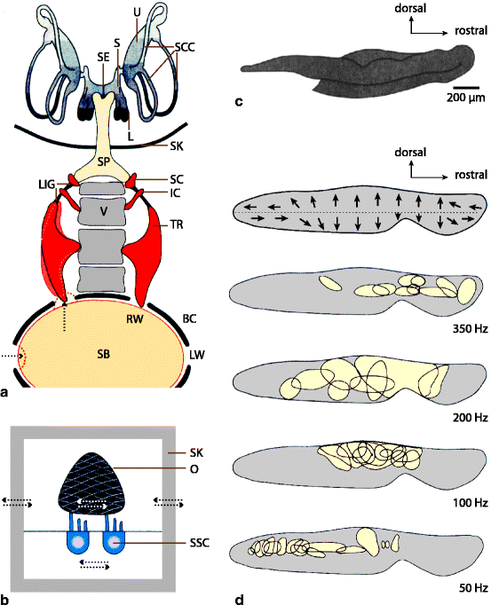

  

  (a) Sound transmission via the Weberian ossicles (TR tripus, IC intercalarium, SC scaphium) from the air (‘sound’) bladder (SB) to the inner ear of ostariophysan fish. The SB is located in a bony capsule (BC). Sound pressure waves enter the capsule through the lateral windows (LW) and stimulate movements of the SB at the rostral windows (RW) in which, on both sides, the TR is inserted. The vibration of the TR travels via the IC and SC to the sinus perilymphaticus (SP; filled with perilymph and reaching into the skull (SK)), and finally to the sinus endolymphaticus (SE; filled with endolymph) in the inner ear. The SE connects to the possible hearing organs, the ­sacculus (S), the lagena (L), and the utriculus (U). LIG ligament, SCC semicircular canals, SK skull, V vertebra. (b) Displacement of sensory cells (SSC) of an otolithic organ in a fish without air bladder. In the near-field of a sound source the skull vibrates relative to the inertial mass of the otolith (O) leading to a displacement of the kinocilium and the stereocilia of the sensory cells. (c) Otolith from the sacculus of a minnow. (d) Orientation of the cilia of the sensory cells in the sacculus of a cod. The main areas of stimulation by tones of different frequencies are also shown (All modified from Tavolga et al. and Ziswiler [47, 54] with permission)

• (c) Fish have several hearing organs. All three ­sensory organs with otoliths in the inner ear – ­sacculus, utriclus, and lagena – and the macula neclecta (without otolith) can function as hearing organs besides their tasks as organs of equilibrium and position control. The sacculus has auditory function most probably in all fish, the other organs contribute in a species-specific way. The crossopterygian fish Latimeria may be the only living species with a basilar papilla, which becomes the main auditory organ in land vertebrates [10]. Figure 17.19b explains the principle function of otolith organs in hearing. In the near field of a sound source the skull vibrates with the sound frequency relative to the inertial mass of the otolith. This relative movement by the sound velocity leads to displacements of the kinocilium and the stereocilia of the hair cells in the rhythm of the sound waveform (e.g., sine wave for low-frequency tones). Depending on the mass to be moved and the shape of the otolith, only relatively low frequencies (f  <  1 kHz) lead to displacements of the cilia and to auditory stimulation. The shape of the otolith together with the orientation of the hair cells and their attachment to the otolith are responsible for local stimulation maxima on the sensory epithelium as a function of the stimulation frequency (Fig. 17.19c, d). This shows that one principle of frequency analysis in auditory organs of vertebrates is already realized in a rather crude way in fish, namely the frequency-place-transformation leading to a tonotopy on the sensory epithelium. The main mechanism of frequency coding in auditory nerve fibers of fish, however, is the phase-locking of spikes to the sound waveform, which is functional up to about 1–2 kHz.

17.4.2 Central Auditory System

Since the hearing organs of fish are also intimately related to the functions of equilibrium and position control, it is difficult to separate these functions in the brain centers for processing information from the inner ear. In addition, central projections of the lateral line system partly overlap areas receiving projections from the inner ear. Therefore, the central auditory system of fish deviates from the diagrams shown in Fig. 17.10 and possible homologies are difficult to be assessed. Reviews can be found in [25, 47, 49].

17.5 Insects

Apart from vertebrates, various insects can hear. Insects use hearing for acoustic communication or to detect the ultrasonic echolocation signals emitted by hunting bats [44]. Some parasitoid flies also employ hearing to locate their hosts, singing crickets [33] and some predatory bushcrickets listen to, and acoustically mimic, the songs of sexually receptive females of certain cicada species to misguide and devour their males [23]. The ability to hear has evolved many times independently within different insect taxa, which all transformed proprioceptive stretch receptor organs into hearing organs [53] (Fig. 17.20). Because of these multiple evolutionary origins, insect hearing organs vastly differ in their anatomies and functional properties, often reflecting adaptations for specific tasks. This diversity, which also extends to the central auditory pathways, may seem bewildering, yet it provides an enticing field for studying evolutionary solutions and innovations of how acoustic signals are processed.

Fig. 17.20

Proprioceptive chordotonal organ and derived tympanal and antennal hearing organs. (a) Proprioceptive chordotonal organs span between different regions of the cuticular exoskeleton and monitor relative movements. The organs can comprise one or more chordotonal sensilla that each consist of one to three mechanosensory neurons and three supporting cells (cap cell, scolopale cell, ligament cell). (b) Tympanal hearing organs are obtained if the cuticule the organ connects to is thinned to a sound-receiving tympanal membrane and backed by a tracheal air sac so that it vibrates in response to sound. (c) In antennal hearing organs, the antenna’s distal part acts as the sound receiver that directly follows the air particle displacements in the sound field. Vibrations of this receiver are picked up by Johnston’s organ, a chordotonal organ in the second antennal segment. The chordotonal sensilla of Johnston’s organ usually perpendicularly connect from different sides to the antennal receiver and are alternately activated as the antenna moves back and forth

17.5.1 Peripheral Auditory System

Some insects detect sounds with mechanosensory ­bristles (Chap. 16), yet the more sophisticated hearing organs that can be found in insects seem all derived from proprioceptive chordotonal organs (Fig. 17.20a). These internal stretch receptors are serially arranged along the insect body and, spanning between different regions of the cuticular exoskeleton, monitor body movements. An auditory function is obtained if the cuticle in one of these regions is made sufficiently compliant to act as a sound receiver that vibrates in response to sound (Fig. 17.20b, c).

With respect to the physical component of the sound wave that sets this receiver into vibration, sound particle velocity-sensitive ears and sound pressure-­sensitive ears can be distinguished. Particle velocity-sensitive ears are known from honeybees, mosquitoes, and certain drosophilid flies, which hear with their antennae [27] (Fig. 17.20c). In these insects, the mobile distal part of the antenna directly follows the particle movement in the sound field, and these vibrations are monitored by Johnston’s organ, the antennal chordotonal organ. Antennal hearing is used to detect the wing-beat sounds of conspecifics; because the sound particle velocity rapidly drops with distance, it allows for intimate sound communication at close range. Pressure-sensitive ears can occur on various parts of the insect body (Fig. 17.21), depending on which of the serially arranged chordotonal organs has been modified for the detection of sound. Modifications include the thinning of one of the cuticular regions the chordotonal organ connects to, so that, when backed with an air sac, a pressure-sensitive tympanal ­membrane is obtained [14] (Fig. 17.20b). In some cases, sound also enters through the tracheal system and acts on both the membrane’s in- and outside, turning the tympanum into a pressure-difference receiver ­measuring cycle-by-cycle the pressure differences resulting from the different phases of a sound wave having traveled slightly different distances when arriving at the tympanum’s outer and inner sides [44]. As explained for amphibia, reptiles, and birds, the mechanical coupling of tympana in a pressure-difference receiver system provides excellent sound localization abilities for these small animals. Tympanal ears allow for hearing at long distances in the kHz range of frequencies. They are found in, e.g., cicadas, grasshoppers, and crickets that communicate with loud sounds and in nocturnal insects such as moths, mantids, and lacewings that are faced with predation by bats.

Fig. 17.21

Sketch of a generalized insect depicting the different body parts on which tympanal ears can be found in certain insect taxa. 1 mouthparts (some sphingid moths), 2 prosternum on the neck’s ventral side (some tachinid flies), 3 tibia of foreleg (crickets, bushcrickets), 4 mesothorax (some corixid water bugs), 5 grove between metathoracic legs (some praying mantids), 6 posterior metathorax (noctuid moths), 7 ventral (pyralid moths) and anterior regions (geometrid moths, drepanid moths) of the first abdominal segment, 8 laterally on the first abdominal segment (grasshoppers), 9 second abdominal segment (cicadas, some uraniid butterflies), 10 dorsal surface of first abdominal segment (tiger beetles), 11 wing base (lacewings), 12 dorsally on prothorax (some scarab beetles)

Insect sound receivers are mechanically tuned to relevant sound frequencies and their vibrations are directly coupled to chordotonal sensory neurons (Fig. 17.20). They transduce the vibrations into ­electrical signals and encode them in action potentials forwarded to the CNS. Sound-induced vibration with amplitudes of less than a nanometer can suffice to activate the neurons [52]. For antennal ears, it has also been shown that the neurons can be motile and actively augment the receiver’s vibrations on a cycle-by-cycle basis, thus increasing the ear’s mechanical susceptibility for sound. The number of neurons per ear varies greatly between insect taxa, ranging from ca. 16,000 in male mosquitoes down to only a single neuron in certain moths. In the mosquitoes, the neurons are radially arranged around the antennal sound receiver, which is used like a joystick to pin down the direction of sound sources, i.e., females flying nearby. This is possible because sound particle velocity is a vectorial quantity so that the receiver vibrates in the direction in which the sound propagates. Moth ears perform less sophisticated tasks, and a single neuron suffices to determine whether a bat is around or not. In some moth ears, a second, less sensitive neuron has been added (Fig. 17.22). If only the more sensitive neuron fires, that bat must be far, and a turning behavior is triggered that brings away the moth from the bat. If the bat should nonetheless come sufficiently close so that its echolocation signals also activate the less sensitive neuron, the moth immediately stops flying and drops down to the ground.

Fig. 17.22

Ultrasound hearing in noctuid moths. Left: Sketch of a moth highlighting the position of the tympanum (red). Right: Frequency tuning of the ear’s two sensory cells and corresponding frequency distribution of the echolocation signals of sympatric bat species. The two sensory cells named A1 and A2 display a similar frequency tuning, yet the A1 cell is more sensitive (Right graph modified from Fullard [11] with permission)

Because sound pressure is a scalar quantity, turning away from the bat requires the use of binaural cues. The most prominent insects using binaural cues are the small parasitoid flies that home in on singing crickets in the dark. Because the two ears that sit on their neck are directly located beside each other, there is little room for using binaural cues (Fig. 17.23). Measured directly in front of the ears with the loudspeaker placed at an angle of 90° from the animal’s midline, interaural intensity differences are virtually zero and interaural time differences are only 1.5 μs, which is smaller than the jitter of the action potentials generated by the receptor cells (ca. 70 μs). The flies nonetheless show exquisite directional hearing, and they manage by using a trick: instead of keeping them separately, they have mechanically coupled the eardrums of their two ears so that they rock like a seesaw over a small ridge. When the sound wave hits the ipsilateral tympanum, it immediately starts to move, making the contralateral tympanum move in the opposite direction (Fig. 17.24). Once initiated, this oscillation continues as long as the sound stimulus lasts. This seesaw mechanisms increases interaural time difference by a factor of about 1,100 at the level of the tympana, which is then further increased by a factor of about 5.5 at the level of the first-order interneuron onto which the receptors converge. Thus, an interaural time difference of only 50 ns resulting from a sound source displaced only 2° from the fly’s midline [24] is enlarged to a 300 μs difference which is close to the threshold of perception.

Fig. 17.23

Mechanically coupled tympana on the neck of a parasitoid fly. Top: Electron micrograph of the two tympana, which are mechanically coupled via a cuticular ridge (Reprinted with permission from Miles et al. [26]). Bottom: Sound-induced deflection of the tympana upon sound stimulation from the right. Downwards movement of the ipsilateral tympanum makes the contralateral one move up, a seesaw mechanism that amplifies binaural cues, allowing the flies to acoustically pinpoint their singing cricket hosts at night (Modified from Robert and Göpfert [33] with permission)

Fig. 17.24

Tonotopic arrangement of auditory receptors in a bushcricket ear. Top: Position of the tympanum on the tibia of the foreleg. Middle: Close-up of the crista acoustica, which comprises ca. 60 receptor cells that gradually decrease in size. Bottom: Corresponding frequency tuning of the receptors, illustrated for three cells at different sites

Like vertebrate hearing organs, the tympanal ears of many insects also decompose sound into frequency components. Bushcrickets, for example, have ears on their front legs that comprise a linear arrangement of some 60 receptor neurons, the crista acoustica (Fig. 17.24). Each neuron has a different best frequency, and this best frequency gradually increases from the crista’s proximal to its distal end. In grasshoppers, the ears sit laterally on the abdomen, and their auditory receptor organ is called Müller’s organ. This organ comprises several groups of receptor cells that differ in their frequency characteristics and with respect to their tympanal attachment sites. At these sites, the tympanum is mechanically tuned to the corresponding frequencies, so that its mechanics provides a frequency map. Like the basilar membrane in our ears, the locust tympanum also propagates travelling waves that, depending on the sound frequency, funnel sound energy to the respective receptor cells [51].

17.5.2 Central Auditory System

Insect auditory receptors are primary sensory cells that send axons to the central nervous system. The axons usually arborize in the ganglia of the body segment that carries the ear. The receptors of the antennal Johnston’s organ synapse in the antennal mechanosensory motor center in the deuterocerebrum of the brain. Tympanal receptors synapse in the ventral thoracic or abdominal ganglia, unless, as is the case in some sphingid moths, they are located on the head. A considerable amount of stimulus processing takes place already in the ventral ganglia [44]. For example, local interneurons with an Ω-shaped morphology (omega neurons of crickets) enhance directional cues by inhibiting the contralateral side. Movements of the animals towards or away from the sound source (positive and negative phonotaxis) critically depend on the action of these interneurons. In some insects, thoracic ganglia are tonotopically organized with regard to the projection areas of the peripheral sensory cells so that the peripheral tonotopy is reproduced there [36].

From the thoracic or abdominal ganglia ascending interneurons forward the preprocessed information to the brain. There, auditory neurons seem rather scattered in insects with tympanal ears, with some preference for the lateral protocerebrum. Female bushcrickets and crickets listening to singing males at night might be attacked by echolocating bats. So they have to discriminate between their species-specific communication sounds and echolocation signals. Based on frequency differences, this discrimination is done in a categorical way in the ventral ganglia leading to either approach or avoidance behavior. The respective information is also forwarded to the brain via parallel ascending pathways [44]. Descending interneurons may prime the ventral ganglia with information from the brain. Apparently, only few synapses are involved in sound processing and response generation. Bushcrickets may start an avoidance response within less than 20 ms after sound onset. More complex behaviors such as phonotaxic approaches of a singing male by a female involve more complex neuronal circuits and require more processing time.

17.6 Other Invertebrates

Detection of far-field sound or pressure waves through specialized structures such as mechanosensory bristles or tympanic organs is not known for nonarthropod invertebrates (see discussion and review [2]).

References

Ashmore J (2008) Cochlear outer hair cell motility. Physiol Rev 88:173–210
Budelmann BU (1992) Hearing in nonarthopod invertebrates. In: Webster DB, Fay RR, Popper AN (eds) The evolutionary biology of hearing. Springer, Berlin Heidelberg New York, pp 141–155
Buser P, Imbert M (1992) Audition. MIT Press, Cambridge
Capranica RR (1976) Morphology and physiology of the auditory system. In: Llinás R, Precht W (eds) Frog neurobiology. Springer, Berlin Heidelberg New York, pp 551–575
Carr CE, Code RA (2000) The central auditory system of reptiles and birds. In: Dooling RJ, Fay RR (eds) Comparative hearing: birds and reptiles. Springer, Berlin Heidelberg New York, pp 197–248
Clack JA, Allin E (2004) The evolution of single- and multiple-ossicle ears in fishes and tetrapodes. In: Manley GA, Fay RR (eds) The evolution of the vertebrate auditory system. Springer, Berlin Heidelberg New York, pp 128–163
Ehret G (1997) The auditory midbrain, a “shunting yard” of acoustical information processing. In: Ehret G, Romand R (eds) The central auditory system. Oxford Univ Press, New York, pp 259–316
Ehret G (2006) Hemisphere dominance of brain function – which functions are lateralized and why? In: van Hemmen JL, Sejnowski TJ (eds) 23 problems in systems neuroscience. Oxford Univ Press, New York, pp 44–61
Fay RR (1988) Hearing in vertebrates: a psychophysics databook. Hill-Fay Assoc, Winnetka
Fritzsch B (1992) The water-to-land transition: evolution of the tetrapod basilar papilla, middle ear, and auditory nuclei. In: Webster DB, Fay RR, Popper AN (eds) The evolutionary biology of hearing. Springer, Berlin Heidelberg New York, pp 351–375
Fullard JH (2006) The evolution of hearing in moths: the ears of Oenosandra boisduvalii (Noctuoidea: Oenosandridae). Aust J Zool 54:51–56
Greenwood DD (1990) A cochlear frequency-position function for several species – 29 years later. J Acoust Soc Am 87:2592–2605
Grothe B, Pecka M, McAlpine D (2010) Mechanisms of sound localization in mammals. Physiol Rev 90:983–1012
Hoy RR, Robert D (1996) Tympanal hearing in insects. Annu Rev Entomol 41:433–450
Kaas JH (2011) The evolution of auditory cortex: the core areas. In: Winer JA, Schreiner CE (eds) The auditory cortex. Springer, Berlin Heidelberg New York, pp 407–427
Kanwal JS, Ehret G (2011) Communication sounds and their cortical representation. In: Winer JA, Schreiner CE (eds) The auditory cortex. Springer, Berlin Heidelberg New York, pp 343–367
Knudsen EI, Konishi M (1978) Space and frequency are represented separately in the auditory midbrain of the owl. J Neurophysiol 41:870–884
Konishi M, Takahashi TT, Wagner H, Sullivan WE, Carr CE (1988) Neurophysiological and anatomical substrates for sound localization in the owl. In: Edelman GM, Gall WE, Cowan WM (eds) Auditory function. The neurobiological bases of hearing. Wiley, New York, pp 721–745
Liberman MC (1978) Auditory-nerve response from cats raised in a low-noise chamber. J Acoust Soc Am 63:442–455
Malmierca MS, Ryugo DK (2011) Descending connections of auditory cortex to the midbrain and brain stem. In: Winer JA, Schreiner CE (eds) The auditory cortex. Springer, Berlin Heidelberg New York, pp 189–208
Manley GA (1990) Peripheral hearing mechanisms in reptiles and birds. Springer, Berlin Heidelberg New York
Manley GA (2000) Cochlear mechanisms from a phylogenetic viewpoint. Proc Natl Acad Sci U S A 97:11736–11743
Marshall DC, Hill KB (2009) Versatile aggressive mimicry of cicadas by an Australian predatory katydid. PLoS One 4:e4185
Mason AC, Oshinsky ML, Hoy RR (2001) Hyperacute directional hearing in a microscale auditory system. Nature 410:686–690
McCormick CA (1992) Evolution of central auditory pathways in anamniotes. In: Webster DB, Fay RR, Popper AN (eds) The evolutionary biology of hearing. Springer, Berlin Heidelberg New York, pp 323–350
Miles RN, Robert D, Hoy RR (1995) Mechanically coupled ears for directional hearing in the parasitoid fly Ormia ochracea. J Acoust Soc Am 98:3059–3070
Nadrowski B, Effertz T, Senthilan PR, Göpfert MC (2011) Antennal hearing in insects – new findings, new questions. Hear Res 273:7–13
Narins PM, Ehret G, Tautz J (1988) Accessory pathway for sound transfer in a neotropical frog. Proc Natl Acad Sci USA 85:1508–1512
Patuzzi R (1996) Cochlear micromechanics and macromechanics. In: Dallos P, Fay RR (eds) The cochlea. Springer, Berlin Heidelberg New York, pp 186–257
Pickles JO (2008) An introduction to the physiology of hearing, 3rd edn. Emerald, Bingley
Pollak GD (1992) Adaptations of basic structures and mechanisms in the cochlea and central auditory pathway of the mustache bat. In: Webster DB, Fay RR, Popper AN (eds) The evolutionary biology of hearing. Springer, Berlin Heidelberg New York, pp 751–778
Rees A, Langer G (2005) Temporal coding in the auditory midbrain. In: Winer JA, Schreiner CE (eds) The inferior colliculus. Springer, Berlin Heidelberg New York, pp 346–376
Robert D, Göpfert MC (2002) Novel schemes for hearing and acoustic orientation in insects. Curr Opin Neurobiol 12:715–720
Robles L, Ruggero MA (2001) Mechanics of the mammalian cochlea. Physiol Rev 81:1305–1352
Romand R, Avan P (1997) Anatomical and functional aspects of the cochlear nucleus. In: Ehret G, Romand R (eds) The central auditory system. Oxford Univ Press, New York, pp 97–191
Römer H (1983) Tonotopic organization of the auditory neuropile in the bushcricket Tettigonia viridissima. Nature 306:60–62
Rosowski JJ (1994) Outer and middle ears. In: Fay RR (ed) Comparative hearing: mammals. Springer, Berlin Heidelberg New York, pp 172–247
Rouiller EM (1997) Functional organization of the auditory pathways. In: Ehret G, Romand R (eds) The central auditory system. Oxford Univ Press, New York, pp 3–96
Scheich H, Ohl FW (2011) A semantic concept of auditory cortex function and learning. In: Winer JA, Schreiner CE (eds) The auditory cortex. Springer, Berlin Heidelberg New York, pp 369–387
Schreiner CE, Langer G (1997) Laminar fine structure of frequency organization in auditory midbrain. Nature 388:383–386
Scott SK (2005) Auditory processing – speech, space and auditory objects. Curr Opin Neurobiol 15:197–201
Smith CA (1981) Recent advances in structural correlates of auditory receptors. Prog Sens Physiol 2:135–187
Spoendlin H (1970) Structural basis of peripheral frequency analysis. In: Plomb R, Smoorenburg GF (eds) Frequency analysis and periodicity detection in hearing. Sijhoff, Leiden, pp 2–36
Stumpner A, von Helversen D (2001) Evolution and function of auditory systems in insects. Naturwissenschaften 88:159–170
Suga N (1990) Cortical computational maps for auditory imaging. Neural Netw 3:3–21
Suga N, Gao E, Zhang Y, Ma X, Olsen JF (2000) The corticofugal system for hearing: recent progress. Proc Natl Acad Sci USA 97:11807–11814
Tavolga WN, Popper AN, Fay RR (eds) (1981) Hearing and sound communication in fishes. Springer, Berlin Heidelberg New York
Terhardt E (1998) Akustische Kommunikation. Springer, Berlin Heidelberg New York
Webb JF, Fay RR, Popper AN (eds) (2008) Fish bioacoustics. Springer, Berlin Heidelberg New York
Weinberger NM (2011) Reconceptualizing the primary auditory cortex: learning, memory and specific plasticity. In: Winer JA, Schreiner CE (eds) The auditory cortex. Springer, Berlin Heidelberg New York, pp 465–491
Windmill JF, Göpfert MC, Robert D (2005) Tympanal travelling waves in migratory locusts. J Exp Biol 208:157–168
Windmill JF, Fullard JH, Robert D (2007) Mechanics of a ‘simple’ ear: tympanal vibrations in noctuid moths. J Exp Biol 210:2637–2648
Yager DD (1999) Structure, development, and evolution of insect auditory systems. Microsc Res Tech 47:380–400
Ziswiler V (1976) Die Wirbeltiere, vol 1. Thieme, Stuttgart
Author information
Authors and Affiliations
Corresponding author
Editor information
Editors and Affiliations
Rights and permissions
Copyright information
© 2013 Springer-Verlag Berlin Heidelberg
About this chapter
Cite this chapter
Ehret, G., Göpfert, M.C. (2013). Auditory Systems. In: Galizia, C., Lledo, PM. (eds) Neurosciences - From Molecule to Behavior: a university textbook. Springer Spektrum, Berlin, Heidelberg. https://doi.org/10.1007/978-3-642-10769-6_17
Download citation
DOI: https://doi.org/10.1007/978-3-642-10769-6_17
Published:
Publisher Name: Springer Spektrum, Berlin, Heidelberg
Print ISBN: 978-3-642-10768-9
Online ISBN: 978-3-642-10769-6
eBook Packages: Biomedical and Life SciencesBiomedical and Life Sciences (R0)