Fault Diagnosis of Rotating Machinery Based on Empirical Mode Decomposition

Abstract

Rotating machinery covers a broad range of mechanical equipment in industrial applications. It generally operates under tough working environment and is therefore subject to faults easily. Vibration signals collected in the working process have valuable contributions for the presentation of conditions of the rotating machinery. Consequently, using signal processing techniques, these faults could be detected and diagnosed. Empirical mode decomposition (EMD) is one of the most powerful signal processing techniques and has been widely applied in fault diagnosis of rotating machinery. This chapter attempts to introduce the recent research and development of EMD in fault diagnosis of rotating machinery, including basic concepts and fundamental theories about EMD methods and improved EMD methods. Moreover, the applications of EMD methods and improved EMD methods in fault diagnosis of common and key components of rotating machinery, like rotors, gears and rolling element bearings, are described in details.

These keywords were added by machine and not by the authors. This process is experimental and the keywords may be updated as the learning algorithm improves.

1 Introduction

Rotating machinery plays an important role in industrial applications. It generally works under a tough environment. Thus rotating machinery can suffer from failures easily, which may decrease the service performance such as manufacturing quality, operation safety, etc., and even cause the entire mechanical system to break down. With rapid development of science and technology, rotating machinery is becoming larger, more precise and more automatic. Its potential faults become more difficult to be detected. Accordingly, the investigations of rotating machinery fault diagnosis have attracted considerable interests in recent years. Vibration signals collected in the working process have valuable contributions for the presentation of conditions of the rotating machinery. Consequently, adopting advanced signal processing techniques to reveal fault characteristics is one of the commonly used strategies in fault diagnosis of rotating machinery [1, 2]. Empirical mode decomposition (EMD) is one of the most advanced signal processing techniques [3], which is proposed as an adaptive time-frequency signal processing method to analyze non-stationary and nonlinear signals. It is based on the local characteristic time scales of a signal and could decompose the signal into a set of complete and almost orthogonal components called intrinsic mode functions (IMFs). The IMFs indicate the natural oscillatory mode imbedded in the signal and serve as the basis functions, which are determined by the signal itself, rather than pre-determined kernels. Thus, it is a self-adaptive signal processing technique that is suitable for nonlinear and non-stationary processes. Since EMD was proposed in 1998, it has been widely utilized and extensively studied in a lot of areas, for example, process control [4, 5], modeling [6,7,8], surface engineering [9], medicine and biology [10], voice recognition [11], system identification [12, 13], etc.

Although EMD largely contributes to the analysis of non-stationary and nonlinear signals, the algorithm itself has some shortcomings [14,15,16], such as end effects, mode mixing, etc. Aiming at these drawbacks, various theoretical analyses and improved EMD methods have been accomplished [17,18,19,20,21,22]. In addition, some improved EMD methods have been applied in the diagnosis of early rub-impact faults of rotors [21, 22], crack faults of gears [23, 24], and single or compound faults of locomotive bearings [25, 26].

This chapter attempts to introduce the recent research and development of EMD in fault diagnosis of rotating machinery. In the rest of this chapter, basic concepts and fundamental theories about EMD methods and improved EMD methods will be presented. In addition, the applications of EMD methods and improved EMD methods in fault diagnosis of rotors, gears and rolling element bearings, which are the common and key components of rotating machinery, will be described in details.

2 Empirical Mode Decomposition

2.1 EMD Algorithm

The EMD algorithm was proposed by Huang et al. and could decompose a signal into a set of IMFs [3]. An IMF is a function that should be satisfied with the following two conditions: (1) in the whole data set, the number of extrema and the number of zero-crossings must either equal or differ at most by one, and (2) at any point, the mean value of the envelope defined by local maxima and the envelope defined by the local minima is zero [3]. An IMF represents the natural oscillatory mode embedded in the signal. A typical IMF is shown in Fig. 1.

Fig. 1

Waveform of a typical IMF

With the simple assumption that any signal consists of different simple IMFs, the EMD method could decompose a signal into some IMF components, which are determined by the signal itself. Thus, it is a self-adaptive signal processing method. Given a signal $x(t)$, the EMD algorithm can be described as follows.

• (1) Initialize: $r_{0} = x(t)$, and $i = 1$.

• (2) Extract the i-th IMF.

  • (a) Initialize: $h_{i(k - 1)} = r_{i}$, $k = 1$.

  • (b) Extract the local maxima and minima of $h_{i(k - 1)}$.

  • (c) Interpolate the local maxima and the minima by cubic spline lines to form upper and lower envelops of $h_{i(k - 1)}$.

  • (d) Calculate the mean $m_{i(k - 1)}$ of the upper and lower envelops of $h_{i(k - 1)}$, as shown in Fig. 2.

    Fig. 2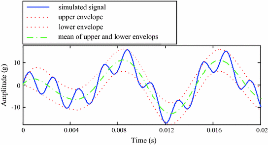

    

    Upper and lower envelops and their mean of a signal

  • (e) Let $h_{ik} = h_{i(k - 1)} - m_{i(k - 1)}$.

  • (f) If $h_{ik}$ is a IMF then set ${\text{IMF}}_{\text{i}} = h_{ik}$, else go to step (b) with $k = k + 1$.

• (3) Define $r_{i + 1} = r_{i} - {\text{IMF}}_{\text{i}}$.

• (4) If $r_{i + 1}$ still has least 2 extrema then go to step (2) else decomposition process is finished and $r_{i + 1}$ is the residue of the signal.

Thus, we can decompose the signal into I IMFs and a residue $r_{I}$, which is the mean trend of $x(t)$. Summing up all IMFs and the final residue $r_{I}$, we get $x(t) = \sum\nolimits_{i = 1}^{I} {c_{i} + r_{I} }$. The frequency bands of IMFs $c_{1} ,c_{2} , \ldots ,c_{I}$ ranges from high to low. The frequency components contained in each frequency band are different and they change with the variation of signal $x(t)$. Figure 3 shows the steps of the EMD algorithm.

Fig. 3

Flow chart of EMD

A simulation is presented here to illustrate the decomposition results of EMD method. Given a signal $x(t)$, it consists of three components: a high-frequency sinusoidal wave, a low-frequency sinusoidal wave and a trend component. We use the EMD method to decompose this signal following the steps in Fig. 3. The decomposed components and the simulated signal $x(t)$ are shown in Fig. 4. From Fig. 4, it can be seen that two IMFs c ₁ and c ₂, and a residue r ₂ are produced. Among them, c ₁ and c ₂ correspond to the two sinusoidal waves with different frequencies and the residue r ₂ reflects the trend component embedded in the simulated signal.

Fig. 4

Illustration of the EMD method

2.2 Problems of EMD

Although EMD largely contributes to the analysis of non-stationary and nonlinear signals, it also has weaknesses as well. For example, EMD produces end effects; the IMFs are not strictly orthogonal to each other; mode mixing sometimes occurs between IMFs.

• (a) End effects

For a clear understanding of the end effects of EMD, we use the simulated signal shown in Fig. 4 to illustrate the end effects. We display the two sinusoidal waves included in the simulated signal and the decomposed IMFs of the simulated signal by EMD in Fig. 5. It is seen that there are distortions at the two ends of IMFs. This phenomenon is called end effects and it is caused by the EMD algorithm itself.

Fig. 5

a Simulated high-frequency sine wave and IMF c ₁, and b simulated low-frequency sine wave and IMF c ₂

• (b) Problem of orthogonality

The decomposed IMFs by EMD are not strictly orthogonal to each other. As we all know, if two components are orthogonal to each other, the dot product between them is zero. Here we also take the IMFs in Fig. 4 as an example. Calculating the dot product between the two IMFs c ₁ and c ₂, we obtain the value of 1.5 instead of zero. This means that IMFs c ₁ and c ₂ are not strictly orthogonal to each other. Moreover, the energy of the two IMFs and the residue can be calculated as 514.6, 515.2 and 1161.8, respectively, which means that the total energy of the three decomposed components is 2191.6. It is not equal to the energy of the simulated signal 2125.8. This indicates that when a signal is decomposed by EMD, the energy is not conservative before and after decomposition.

• (c) Mode mixing

EMD method has another obvious shortcoming called mode mixing. The mode mixing of EMD is defined as a single IMF including oscillations of dramatically disparate scales, or a component of a similar scale residing in different IMFs.

To illustrate the problem of mode mixing in EMD, another simulated signal $x(t)$ is considered in this section. The simulated signal is shown in Fig. 6a. There is a sine wave of 36 Hz and small impulses included in this simulated signal. Therefore, it is a combined signal and actually consists of two components. Utilizing EMD on the signal, the decomposed results are shown in Fig. 6.

Fig. 6

Decomposition result with EMD: a the simulation signal, b IMF c ₁, and c IMF c ₂

From Fig. 6, we can see that mode mixing is occurring between IMFs c ₁ and c ₂ since there are neither indications of a sinusoidal wave nor indications of small impulses. The sinusoidal wave and the impulses are decomposed into the same IMF (c ₁). That is to say, these two IMFs obtained by EMD are distorted obviously and both IMFs c ₁ and c ₂ of EMD fail to represent the characteristics of signal $x(t)$ accurately. This is a typical problem of mode mixing.

Mode mixing of EMD is a result of signal intermittency. To solve the problem of mode mixing in the original EMD, ensemble empirical mode decomposition (EEMD), was developed by Wu and Huang by adding noise to the investigated signal [20]. A brief introduction of EEMD is given in the next section.

Besides the end effects and mode mixing mentioned above, the EMD method has some other weaknesses, such as lacking a theoretical foundation, sifting stop criterion, extremum interpolation, etc. More details can be found in Refs. [14,15,16].

2.3 Hilbert-Huang Transform

Hilbert-Huang transform (HHT) mainly consists of two steps: EMD and Hilbert transform. EMD can decompose a signal into a collection of IMFs, which are almost monocomponent. Hilbert transform is defined as the convolution of signal $x(t)$ with $1/t$, shown in Eq. (1). Through the Hilbert transform, local properties of $x(t)$ are emphasized.

$$y(t) = \frac{1}{\pi }\int\limits_{ - \infty }^{ + \infty } {\frac{x(t)}{t - \tau }} d\tau$$

(1)

Combining $x(t)$ and $y(t)$,we can obtain the analytic signal $z(t)$ of $x(t)$

$$\left\{ {\begin{array}{*{20}l} {z(t) = x(t) + iy(t) = a(t){\text{e}}^{i\phi (t)} } \hfill \\ {a(t) = \sqrt {x^{2} (t) + y^{2} (t)} } \hfill \\ {\varphi (t) = \arctan (y(t)/x(t))} \hfill \\ \end{array} } \right.$$

(2)

where $a(t)$ is the instantaneous amplitude of $x(t)$, which reflects how the energy of $x(t)$ varies with time $t$, and $\varphi (t)$ is the instantaneous phase of $x(t)$. If the signal $x(t)$ is monocomponent, then the time derivative of instantaneous phase $\varphi (t)$ will be the physical meaning of instantaneous frequency $\omega (t)$ of the signal $x(t)$. Then the instantaneous frequency $\omega (t)$ is given as

$$\omega (t) = \frac{{{\text{d}}\varphi (t)}}{{{\text{d}}t}}$$

(3)

As discussed before, EMD can generate almost monocomponent IMFs, which provides an opportunity for the instantaneous frequency applied to complicated signals. For the signal $x(t)$, $I$ IMFs are produced by EMD. Applying the Hilbert transform to each IMF, and calculating the instantaneous frequency and amplitude, we can express signal $x(t)$ in the following representation:

$$x(t) = \sum\limits_{i = 1}^{I} {a_{i} (t)\exp \left( {j\int {\omega_{i} (t){\text{d}}t} } \right)}$$

(4)

Therefore, based on the IMFs obtained by EMD, the Hilbert transform generates a time-frequency-energy distribution to depict signal $x(t)$. The EMD-based Hilbert transform is called Hilbert-Huang transform (HHT).

3 Improved EMD Methods

3.1 EEMD Method

As we all know, mode mixing is a typical problem of EMD method. When the problem of mode mixing occurs, an IMF can cease to have physical meaning by itself, suggesting falsely that there may be different physical processes represented in a mode [3]. To overcome this problem, ensemble empirical mode decomposition (EEMD) was proposed based on the statistical properties of white noise. In this new method, the true IMFs are defined as the mean of an ensemble of trials which consist of the decomposition results of the signal plus a normally distributed white noise with a constant standard deviation [20]. When the white noise is decomposed by EMD, EMD behaves likes a dyadic filter bank: the Fourier spectra of various IMFs collapse to a single shape along the axis of the logarithm of frequency [27]. In addition, the result provided by Flandrin, Gonçalvès, and Rilling demonstrated that the white noise could help data analysis in the EMD method [28]. In the process of EEMD, different white noise with zero mean and a constant standard deviation is added to the original signal and the combined signal is decomposed using EMD method in each trial. When the white noise is added to the signal, the components in different in different scales of the signal are automatically projected onto proper scales of reference established by the white noise in the background. The influence of the added noise can be decreased or even completely canceled out in the ensemble mean of enough trials. Therefore, the ensemble mean is treated as the true answer for the reason that only the signal is reserved when more and more trials are carried out in the ensemble process. The principle of EEMD advanced here is on the basis of the observations in the following [20].

• (1) A collection of white noise cancels each other out in an ensemble mean; hence, only the signal can be reserved in the final noise-added signal ensemble mean.

• (2) White noise is used to force the ensemble to find all possible solutions; it makes the signals of different scale reside in the corresponding IMFs, and the resulting ensemble mean can be more meaningful.

• (3) The decomposition with truly physical meaning of EMD is not the one without noise; it is designated to be the ensemble mean of a large number of trials consisting of the noise-added signal. More detailed description of EEMD can be found in Ref. [20].

Based on the principle and observations as mentioned earlier, the EEMD algorithm is given below and Fig. 7 is its flow chart.

Fig. 7

Flow chart of EEMD

• 1. Initialize the number of ensemble, M, the amplitude of the added white noise, and $m = 1$.

• 2. Perform the m-th trial on the signal added white noise.

  • (a) Add a white noise series with the given amplitude to the signal to be studied

    $x_{m} (t) = x(t) + n_{m} (t)$, where $n_{m} (t)$ indicates the mth added white noise series, and $x_{m} (t)$ represents the noise-added signal of the m-th trial.

  • (b) Decompose the noise-added signal $x_{m} (t)$ into N IMFs, $c_{n,m}$($n = 1,2, \ldots ,N$), using EMD, where $c_{n,m}$ denotes the nth IMF of the m-th trial, and N is the number of IMFs.

  • (c) If $m < M$ then go to step (a) with $m = m + 1$. Repeat steps (a) and (b) again and again with different white noise series but having the same amplitude each time.

• 3. Calculate the ensemble mean $y_{i}$ of the M trials for each IMF

  $$y_{n} = \frac{1}{M}\sum\limits_{m = 1}^{M} {c_{n,m} } ,\quad n = 1,2, \ldots ,N,\quad m = 1,2, \ldots ,M$$

  (5)

• (4) Report the mean $y_{n}$ ($n = 1,2, \ldots ,N$) of each of the N IMFs as the final IMF.

In order to demonstrate the improvement of EEMD method, the simulated signal in Fig. 6a is decomposed again using EEMD with the ensemble number 100 and the added noise amplitude 0.01 time standard deviation of the signal. The original signal is a sine wave of 36 Hz attached by small impulses. The decomposition results of EEMD method are shown in Fig. 8.

Fig. 8

a The simulated signal; b and c the decomposition results of EEMD

It has been concluded from Fig. 6 that the mode mixing is serious between the two IMFs obtained by EMD. However, it can be seen from Fig. 8b, c that the two components contained in the signal are decomposed into two IMFs perfectly using EEMD. IMF c ₁ in Fig. 8b denotes the impulse components and IMF c ₂ in Fig. 8c indicates the sine wave. Therefore, EEMD is able to overcome the mode mixing problem existing in EMD method and achieve an improved decomposition with physical meaning.

When EEMD method is used, parameters such as the number of ensemble and amplitude of the added noise need to be set reasonably. The following part will discuss the choice of the two parameters.

• (a) The number of ensemble

The relationship between the ensemble number and the amplitude of the added white noise is given in the following equations [20].

$$e = \frac{a}{\sqrt N }$$

(6)

or

$$\ln e + \frac{a}{2}\ln N = 0$$

(7)

where $N$ is the number of ensemble, $a$ is the amplitude of the added white noise, and $e$ is the standard deviation of error, which is defined as the difference between the input signal and the corresponding IMFs.

In the process of EEMD method, small amplitude of the added white noise may lead to a small error. However, if the amplitude of added noise is too small, it may not change the distribution of extrema that the EEMD method relies on. This is true when the investigated signal has a large gradient. Thus, the amplitude of the added noise should not be too small for the effectiveness of EEMD method. On the other hand, the error caused by the added white noise could always be reduced to a quite small even negligible level by increasing the number of ensemble. Generally, an ensemble number of a few hundred will lead to an exact result, and the remaining noise would cause less than a fraction of one percent of error if the added noise has the amplitude that is a fraction of the standard deviation of the investigated signal [20].

• (b) The amplitude of the added white noise

The investigation in references indicated that EMD is a noise-friendly method [20]. In addition, increasing noise amplitudes and ensemble numbers changes the decomposition results little as long as the amplitude of added noise is moderate and the ensemble number is large enough.

The fact is that when the amplitude of noise increases, the number of ensemble should increase to reduce the influence of the added noise in the decomposed results. It is suggested that the amplitude of the added white noise is about 0.2 time standard deviation of the investigated signal [20]. However, it is not always the proper amplitude of the added noise for any cases. Generally, when the signal is dominated by high frequency components, the noise amplitude needs to be smaller. On the contrary, when the signal is dominated by low frequency components, the noise amplitude should be larger. However, there is no a specific equation reported in the literature to guide the choice of the noise amplitude until now. Thus, for an investigated signal, different noise levels should be tried to select the appropriate one.

3.2 AEEMD Method

As stated above, EEMD, as a noise-assisted data analysis method, is aimed to solve the problem of mode mixing in EMD [20]. With the help of the added finite white noise, EEMD is supposed to eliminate the mode mixing problem [21]. The performance of EEMD, however, depends on the parameters adopted in the process of decomposition, such as the sifting number, and the amplitude of the added noise. In fact, these parameters were set as constant values whether the signal to be investigated contains high or low components in most current studies on EEMD [14]. Therefore, the problem of mode mixing is not solved completely and further work need to be done to improve the performance of EEMD.

On the basis of the investigation of the filtering behavior of EMD/EEMD and the relation between the signal frequency components and the amplitude of the added noise, a new adaptive ensemble empirical mode decomposition method (AEEMD) is proposed [24]. The new method adaptively selects the sifting number and decides the amplitude of the added noise according to the signal frequency components in decomposition process. By adopting the two parameters, the performance of EEMD is going to be improved in feature extraction and fault diagnosis.

In the process of EEMD, high and low frequency components have different sensitivity to noise. Therefore, larger noise and more sifting number had better be adopted when high-frequency IMFs are extracted, while smaller noise and less sifting number had better be used when low-frequency IMFs are extracted. To satisfy this requirement for noise, different kinds of noise are tried and tested. The result shows that the noise whose amplitude changes with its frequency in sine form performs best. Therefore, the noise of this form is constructed and utilized in AEEMD in place of white noise adopted in the original EEMD. Figure 9 gives the frequency spectrum of the constructed noise, in which $f_{\text{s}}$ represents the sampling frequency and $e$ denotes the amplitude at the highest frequency. On the other hand, EMD method is an effective self-adaptive dyadic filter bank when applied to white noise. Therefore, the sifting number for each IMF is adaptively set following Eq. (8). Figure 10 gives the flow chart of AEEMD algorithm. The concrete steps are as follows.

Fig. 9

Spectrum of the noise constructed

Fig. 10

Flowchart of AEEMD

• (1) Initialize the amplitude $e$ of the highest frequency of the added noise, the number of ensemble $M$, generally $M = 100$ and $e = 0.2$. Let $m = 1$.

• (2) Calculate the number of IMFs based on the signal length [20]

  $$I = \log_{2} L - 1$$

  (8)

  where $L$ is the signal length.

• (3) Adaptively set the sifting number $p_{i}$ for the i-th IMF according to the following equation.

  $$p_{i} = 2^{{(I - i^{2} )}} + 2, \quad i = 1,2, \ldots ,I$$

  (9)

• (4) Construct the noise as shown in Fig. 9 and add it to the signal to be investigated.

• (5) Perform EMD on the added-noise signal and obtain the m-th decomposition result $a_{i,m}$.

• (6) If $m < M$ then go to step (4) with $m = m + 1$. Repeat steps (4) and (5).

• (7) Calculate the ensemble mean $a_{i}$ of the $M$ trials for each IMF and report the mean as the final IMF.

  $$a_{i} = \frac{1}{M}\sum\limits_{m = 1}^{M} {a_{i,m} } ,\quad i = 1,2, \ldots ,I,\quad m = 1,2, \ldots ,M$$

  (10)

To demonstrate the effectiveness of AEEMD method, a simulation signal is constructed. For the reason that modulation and impact are two typical fault events in rotating machinery, the simulation signal contains modulation as well as impact components. What is more, it also consists of a high-frequency sinusoidal wave and a low-frequency sinusoidal wave respectively to represent certain rotating frequencies of machinery. Therefore, there are four components having different physical meaning in the simulation signal. The four components and the simulation signal combined by them are shown in Fig. 11a–e, respectively.

Fig. 11

a–d Four components, e Simulation signal

AEEMD method is used to decompose the simulation signal and the decomposition results are shown in Fig. 12. It can be seen from the result that IMFs 1–4 correspond to the impact component, the modulation component, the high-frequency sinusoidal wave and the low-frequency sinusoidal wave respectively.

Fig. 12

IMFs using AEEMD for the simulation signal

Comparing the decomposed IMFs in Fig. 12 with the real components in Fig. 11a–d, it can be inferred that the different components embedded in the simulation signal are extracted accurately by AEEMD. For comparison, the simulation signal is analyzed using the original EMD too and the decomposition result is displayed in Fig. 13. It is seen that the problem of mode mixing between different components is very serious and there are distortions for some IMFs. For example, the first IMF contains not only the impact component but also the modulation component. This result illustrates that the original EMD fails to produce the reasonable decomposition. Based on the above simulation and comparison, it could be inferred that AEEMD performs more effective than the original EMD, by adding noise with the amplitude varying as a sinusoidal relation with its frequency into the signal, and adaptively changing the sifting number for different IMFs.

Fig. 13

IMFs using the original EMD for the simulation signal

3.3 CEEMDAN Method

EEMD is mainly to alleviate the problem of mode mixing caused by EMD [20, 29], however, it still has some shortcomings. For example, the EEMD method decomposes a signal adding the white Gaussian noise, and the final IMFs are obtained by averaging the IMFs. This would probably lead to some residual noise in the reconstructed signal. In addition, if the white Gaussian noise in each decomposition process is added with different amplitudes, it probably may produce a different number of IMFs, which makes it difficult for the averaging [30, 31].

To overcome the above shortcomings of EEMD, Torres et al. proposed an algorithm called a complete ensemble empirical mode decomposition with adaptive noise (CEEMDAN) [30]. Furthermore, Colominas et al. continued to make improvements on CEEMDAN [31]. In this improved CEEMDAN method, a particular noise $E_{k} (w^{(i)} )$ instead of the white Gaussian noise is added at each stage of the decomposition, where $E_{k} (w^{(i)} )$ means the kth IMF of the white Gaussian noise decomposed by EMD. Moreover, this method defines the true IMF as the difference between the current residue and the average of its local means. As a result, the problem of remaining noise in IMFs is much alleviated and the problem of the final averaging because of a different number of IMFs is solved.

Let $M( \cdot )$ represent the operator that produces the local means of the signal $x$, and $E_{k} ( \cdot )$ be the operator which produces the kth IMF decomposed by EMD. Obviously, there exists a relation that $E_{1} (x) = x - M(x)$. Considering the relation between the first IMF $c_{1}$ and the residue $r_{1}$:$c_{1} = x - r_{1}$, $c_{1} = \frac{1}{I}\sum\nolimits_{i = 1}^{I} {E_{1} (x)} = x - \frac{1}{I}\sum\nolimits_{i = 1}^{I} {M(x^{(i)} )}$, where I means the averaging number of IMFs, there exists $\frac{1}{I}\sum\nolimits_{i = 1}^{I} {M(x^{(i)} )} = r_{1}$. The decomposition using CEEMDAN is based on the following principles [30, 31] and a flow chart of the CEEMDAN algorithm is shown in Fig. 14.

Fig. 14

Flow chart of the CEEMDAN algorithm

• Step 1. Add $E_{1} (w^{(i)} )$ to the original signal $x$, $x^{(i)} = x + \beta_{0} E_{1} (w^{(i)} )$, where $w^{(i)}$ indicates the i-th added white noise.

• Step 2. Use EMD to calculate the local means of $x^{(i)}$ and average them for the first residue, $r_{1} = \frac{1}{I}\sum\nolimits_{i = 1}^{I} {M(x^{(i)} )}$, then calculate the first IMF $c_{1}$ as $c_{1} = x - r_{1}$.

• Step 3. Obtain the second IMF $c_{2}$ as $c_{2} = r_{1} - r_{2}$, where $r_{2} = \frac{1}{I}\sum\nolimits_{i = 1}^{I} {M(r_{1} + \beta_{1} E_{2} (w^{(i)} ))}$.

• Step 4. Similarly, the k-th IMF $c_{k}$ is computed as $c_{k} = r_{k - 1} - r_{k}$, where $r_{k} = \frac{1}{I}\sum\nolimits_{i = 1}^{I} M (r_{k - 1} + \beta_{k - 1} E_{k} (w^{(i)} )),\quad k = 2,{ 3} \, \ldots \, {\text{N}}.$

The coefficients $\beta_{k}$ represent the selection of the SNR at each stage, where $\beta_{k} = \varepsilon_{0} {\text{std}}(r_{k} )$.

To illustrate the decomposition difference between EEMD and CEEMDAN, a simulated signal $x(t)$ is implemented here. There are four components involved in this signal: a high-frequency sinusoidal wave, a low-frequency sinusoidal wave, an impact component and a modulation component. The simulated signal and the four components are shown in Fig. 15a–e, respectively.

Fig. 15

Four components and the simulated signal: a The simulated signal and b–e The four components

According to Refs. [20, 32], when the value of $\varepsilon_{0}$ is close to 0.2, it often has a remarkable performance of the decomposition results. Consequently, we choose the noise amplitude $\varepsilon_{0} = 0.2$ and the ensemble size $I = 100$ in the decomposition of CEEMDAN. The decomposed results of the simulated signal using EMD method and the CEEMDAN method are shown in Figs. 16 and 17, respectively. The components (a–d) in Fig. 16 correspond to high-frequency sinusoidal wave, low-frequency sinusoidal wave, the impact and the modulation component, respectively. It can be seen that the high-frequency sinusoidal wave is mixed with the low-frequency sinusoidal wave and the impact component is mixed with the modulation component obviously. In Fig. 17, it is seen that the individual components hidden in the simulated signal can be extracted using the method based on CEEMDAN. Especially, the impact component and the modulation component are presented clearly in the third and the forth IMF with an accurate waveform, respectively.

Fig. 16

Decomposed components of the simulated signal using EMD

Fig. 17

Decomposed components of the simulated signal using the CEEMDAN method

4 Fault Diagnosis of Rotating Machinery Using EMD Based Methods

4.1 Fault Diagnosis of Rotors

A power generator plays an important role in energy supply. It has a great meaning to diagnose the faults occurring in the power generator to guarantee the regular energy supply, avoiding the economic loss and saving the production cost. A structure sketch of a power generator in a thermal-electric plant in China is given in Fig. 18. This machine set is composed of a high pressure cylinder, a low pressure cylinder, a motor and an exciter.

Fig. 18

Structure sketch of the power generator

A certain day, it was found that the high pressure cylinder vibrated so intensely that the virtual value of vibration signal exceeded the safety threshold, and then the online monitoring system began to sound the alarm. In the later one month, the machine vibrated even more violently. When the power generator was stopped to be maintained, it was found that one of the bearing bushes of the machine set had been broken. In order to identify the fault pattern, the vibration signal was collected by a vibration velocity transducer fixed on the high pressure cylinder, which is shown in Fig. 19. The signal length is 1024, and the sampling frequency is 2000 Hz. The rotating frequency of the machine set is 50.78 Hz.

Fig. 19

Vibration signal collected from the high pressure cylinder

First, the vibration signal was decomposed using EMD method, and the first six IMFs of the decomposed results are given in Fig. 20. A series of impulses could be seen in some local components of IMFs c1 and c2. Therefore, it can be inferred that periodic impacts occur in the high pressure cylinder.

Fig. 20

Decomposed result of the vibration signal of the high pressure cylinder with EMD

However, what is the reason that caused the impacts between the rotor and the bearing bushes? Unfortunately, it is very difficult to answer this question according to the information provided by the IMFs of EMD owing to mode mixing occurring between different IMFs. In addition, there is no more fault information to clarify the fault cause.

To overcome the above difficulty, the CEEMDAN method with the ensemble number of 100 and the white noise amplitude of 0.3 time standard deviation of that of the vibration signal is applied to the signal decomposition. The decomposition results are given in Fig. 21. It can be clearly seen that each IMF has its real physical meaning. IMF c ₁ corresponds to the added white noise. IMFs c ₂ and c ₃ indicate impulse components. IMF c ₄ is the rotating frequency component of the machine set whose value is 50.78 Hz. IMF c ₅ is a component of 25.39 Hz, which is the half rotating frequency of the machine set.

Fig. 21

Decomposed result of the vibration signal of the high pressure cylinder with EEMD

It can be inferred that the fault pattern is not oil whirl in this machine set because oil whirl usually manifests itself by frequencies ranging from 42 to 48% of the rotating frequency of the rotor. In a rotor system, both looseness and rub behave themselves by the half rotating frequency. For the reason that there are impacts between the rotor and the bearing bushes, we can conclude that the fault of the power generator is the rub-impact pattern. That implies that the rotor system of the high pressure cylinder rub and at the same time impact the bearing bushes when the power generator is operating. Then impulse components are generated. Finally, the intense impacts broke one of the bearing bushes.

4.2 Fault Diagnosis of Gears

In modern industry, planetary gear boxes are widely used as a kind of special gear transmission structures owing to their advantages such as large transmission ratio, strong load-bearing capacity. They have big difference with fixed-axis gearboxes and exhibit unique behaviors, which increase the difficulty of fault diagnosis in planetary gearboxes [33,34,35].

In this section, experiments are conducted on a planetary gearbox test rig and vibration signals are collected to demonstrate the effectiveness of the adaptive EEMD in diagnosing gear faults. The planetary gearbox test rig consisted of two gearboxes, a 3-hp motor for driving the gearboxes, and a magnetic brake for loading. There were a planetary gearbox and a fixed-axis gearbox in the test rig. An inner sun gear is surrounded by several rotating planet gears, and a stationary outer ring gear in the planetary gearbox, which is our concern [33]. To simulate gear faults, a crack at the tooth root of one planetary gear is created in our experiments.

An accelerometer is fixed on the planetary gearbox casing to collect the vibration signals. The motor speed is about 20 Hz and the sampling frequency is set as 5120 Hz. The experimental parameters and the characteristic frequencies of the planetary gearbox are shown in Table 1. It can be seen from the table that the rotating frequency of one planetary gear is 2.5 times as large as that of the carrier. Therefore, when the carrier rotates 2 cycles, the planetary gear meshes 5 periods with the ring gear, i.e. 200 teeth. This tooth number is twice as large as that of the ring gear. That is to say, the ring gear meshes 2 periods with the planetary gear. In other words, the planetary gear returns to the initial position when the carrier rotates 2 cycles. For the carrier to finish rotating 2 cycles, it takes 2/3.33 = 0.6 s.

Table 1 Parameters and characteristic frequencies of the planetary gearbox

The vibration signal collected from the test rig with the cracked planetary gear is shown in Fig. 22a and its frequency spectrum is shown in Fig. 22b. It can be seen that there are a series of impulses in the time-domain waveform. The period of the impulses is nearly $t = 0.1$ s which means that the frequency of the impulses is about 10 Hz. There are three planetary gears in planetary gearbox and they pass the fixed accelerometer in turn. Therefore, the pass frequency of the planetary gears equals 3 times as large as the rotating frequency of the carrier, i.e. 10 Hz. It is apparent that the impulses in the time-domain waveform are caused by the rotation of the carrier, and they are normal vibration components of the gearbox. Unfortunately, it is difficult to extract any fault characteristics besides these impulses for the reason that the fault features of the planetary gearbox are buried by the normal vibration components. The frequency spectrum of the vibration signal in Fig. 22b shows that there are rich sidebands around the mesh frequency and the interval of the sidebands is 3.33 Hz, which equals the rotating frequency of the carrier. Obviously, it is not the fault characteristics either. Therefore, the fault features of the cracked planetary gear cannot be found from the time-domain waveform or its frequency spectrum.

Fig. 22

Experimental signal a time-domain waveform, and b frequency spectrum

The adaptive EEMD method is used to process the above signal to extract the fault features of the cracked planetary gear. Among the IMFs decomposed by adaptive EEMD, the first IMF contains the richest information and consequently it is selected for further analysis. Figure 23 shows the detail of IMF1 and it can be seen that there are impulses with the period $T = 0.6$ s. It can be concluded that once the carrier rotates 2 cycles, the cracked planetary gear returns to the initial position. As a result, the fault period of the cracked planetary gear doubles the rotating period of the carrier, i.e. 0.6 s. That means that the impulse component with the period $T = 0.6$ s is resulted by the cracked planetary gear. Therefore, the adaptive EEMD method can extract the fault characteristics effectively. For comparison, the same signal is decomposed by original EEMD and the first IMF is shown in Fig. 24. In can be seen that there are also periodic impulses in the waveform of the IMF, the impulse ($T = 0.6$ s) caused by the cracked gear and those ($t = 0.1$ s) caused by the rotation of the carrier. However, these impulses are decomposed in the same IMF which means the mode mixing happens. It can be concluded from the comparisons that the adaptive EEMD is more effective than the original EEMD in fault characteristics extraction of the planetary gearbox.

Fig. 23

First IMF extracted by the adaptive EEMD method

Fig. 24

First IMF extracted by the original EEMD method

4.3 Fault Diagnosis of Rolling Element Bearings

In this section, to demonstrate the effectiveness of the CEEMDAN based method, an experiment on a test bench of locomotive rolling element bearings was conducted. The detailed information of the test bench can be seen in Ref. [2]. The parameters and fault characteristic frequencies of the bearings are listed in Table 2.

Table 2 Parameters and fault characteristic frequencies of the locomotive rolling element bearing

It is known that even though a serious single fault occurs on the bearing, periodical impulses characterizing the fault can be submerged by the heavy noise, which may be even worse for compound faults. This is mainly because in rolling element bearings, once compound faults occur, different fault characteristics always couple with each other. Then the fault characteristics of compound faults turned to be complicated and difficult to be extracted, and the common used methods like Fourier spectrum analysis probably will fail to work. Thus for the demonstration of the CEEMDAN method in the fault diagnosis of bearings, we choose a bearing with compound faults on the outer race and the roller.

A vibration signal was collected from the test bench with a sampling frequency of 12800 Hz and a signal length of 16,384 data points. The waveform of the signal and its corresponding Fourier spectrum is given in Fig. 25. The outer race and the roller fault characteristic frequencies of the bearing can be calculated as 44.5 and 19.94 Hz, respectively, since the rotation speed is 370 rpm. Obviously, in Fig. 25, neither the periodic impulses related to faults in the time-domain waveform nor the fault characteristic frequencies in the Fourier spectrum can be observed. The Fourier spectrum analysis fails to detect the compound faults.

Fig. 25

a Vibration signal of a bearing with compound faults, and b Fourier spectrum

To reveal the fault characteristics, EEMD is used to extract the fault characteristics from the signal. 16 IMFs are obtained after the decomposition. However, there is no obvious fault indication at the characteristic frequency of 44.5 and 19.94 Hz from the first 10 IMFs and their corresponding Fourier spectra in Fig. 26. After carefully checked the Fourier spectra of the 8th and 9th IMFs given in Fig. 27, we found two obvious peaks at the frequency of 58.59 and 27.34 Hz. These two frequencies, however, are neither the outer race fault characteristic frequency of 44.5 Hz nor the roller fault characteristic frequency of 19.94 Hz. Hence, the EEMD method fails to extract fault characteristics and diagnose the compound faults of this rolling element bearing.

Fig. 26

Decomposition results of the vibration signal of a bearing with compound faults using EEMD: a The IMFs, and b The Fourier spectra of IMFs

Fig. 27

a Fourier spectrum of the 8th IMF, and b Fourier spectrum of the 9th IMF using EEMD

For comparison, the CEEMDAN based method is applied to analyze the signal using the same noise amplitude and ensemble size in the EEMD method. There are totally 15 IMFs obtained by CEEMDAN and Fig. 28 shows the first 10 IMFs and their Fourier spectra. By examining each Fourier spectrum, we find that there are peaks at the outer race and the roller fault characteristic frequency (45.31 and 20.31 Hz) in the Fourier spectra of the 9th and 10th IMFs, shown in Fig. 29a, b, respectively. Therefore, based on the extracted fault characteristics using the CEEMDAN-based method, the compound faults of this bearing are diagnosed.

Fig. 28

Decomposition results of the vibration signal of a bearing with compound faults using the CEEMDAN method: a the IMFs, and b the Fourier spectra of IMFs

Fig. 29

a Fourier spectrum of the 9th IMF, and b Fourier spectrum of the 10th IMF using the CEEMDAN method

5 Conclusions

In this chapter, the basic theory of EMD and improved EMD methods, such as EEMD method, adaptive EEMD method, etc., are presented. In addition, the applications of these methods in fault diagnosis of rotating machinery, including rotors, gears and rolling element bearings, are described in details.

• (a) The empirical mode decomposition (EMD) method has a good performance in the analysis of nonlinear and non-stationary signals. However, it is often subject to some problems, like end effects and mode mixing, etc. Thus the decomposed IMFs sometimes are unable to reflect the fault characteristics in fault diagnosis of rotating machinery precisely.

• (b) To overcome the shortcomings of EMD, a lot of new methods based on EMD are proposed to diagnose rotating machinery improve the EMD method. These methods are developed mainly by adding different kinds of white Gaussian noise to improve the extrema distribution of the signal.

• (c) The EMD and improved EMD methods have been applied in the fault diagnosis of rotating machinery. EMD sometimes cannot detect the fault in the machinery, while the improved methods promote the performance of EMD in different aspects. These methods have been proven to be effective in the diagnosis of rotors, gears and rolling element bearings.

References

Fan X., Zuo M.J., “Machine fault feature extraction based on intrinsic mode functions,” Measurement Science and Technology, 2008, 19:045105.
Lei Y., He Z., Zi Y., Chen X., “New clustering algorithm-based fault diagnosis using compensation distance evaluation technique,” Mechanical Systems and Signal Processing, 2008, 22:419–435.
Huang N.E., Shen Z., Long S.R., Wu M.C., Shih H.H., Zheng Q., “The empirical mode decomposition and the Hilbert spectrum for nonlinear and non-stationary time series analysis,” Proceedings of the Royal Society of London A: Mathematical, Physical and Engineering Sciences, 1998, 903–995.
Srinivasan R., Rengaswamy R., Miller R., “A modified empirical mode decomposition (EMD) process for oscillation characterization in control loops,” Control Engineering Practice, 2007, 15:1135–1148.
Luo L., Yan Y., Xie P., Sun J., Xu Y., Yuan J., “Hilbert–Huang transform, Hurst and chaotic analysis based flow regime identification methods for an airlift reactor,” Chemical Engineering Journal, 2012, 181:570–580.
Xu G., Tian W., Qian L., “EMD-and SVM-based temperature drift modeling and compensation for a dynamically tuned gyroscope (DTG),” Mechanical Systems and Signal Processing, 2007, 21:3182–3188.
Guo Z., Zhao W., Lu H., Wang J., “Multi-step forecasting for wind speed using a modified EMD-based artificial neural network model,” Renewable Energy, 2012, 37:241–249.
Tang J., Zhao L., Yue H., Yu W., Chai T., “Vibration analysis based on empirical mode decomposition and partial least square,” Procedia Engineering, 2011, 16: 646–652.
Zhang Z., Zhang Y., Zhu Y., “A new approach to analysis of surface topography,” Precision Engineering, 2010, 34:807–810.
Charleston-Villalobos S., Gonzalez-Camarena R., Chi-Lem G., Aljama-Corrales T., “Crackle sounds analysis by empirical mode decomposition,” IEEE Engineering in Medicine and Biology Magazine, 2017, 26:40–47, 2007.
Ambikairajah E., “Emerging features for speaker recognition,” 2007 6th International Conference on Information, Communications & Signal Processing, 2007, pp. 1–7.
Yang Y., Chang K., “Extraction of bridge frequencies from the dynamic response of a passing vehicle enhanced by the EMD technique,” Journal of Sound and Vibration, 2009, 322:718–739.
Zhang H., Qi X., Sun X., Fan S., “Application of Hilbert-Huang transform to extract arrival time of ultrasonic lamb waves,” International Conference on Audio, Language and Image Processing, 2008, pp. 1–4.
Rato R., Ortigueira M., Batista A., “On the HHT, its problems, and some solutions,” Mechanical Systems and Signal Processing, 2008, 22:1374–1394.
Chen G., Wang Z., “A signal decomposition theorem with Hilbert transform and its application to narrowband time series with closely spaced frequency components,” Mechanical Systems and Signal Processing, 2012, 28:258–279.
Rilling G., Flandrin P., Goncalves P., “On empirical mode decomposition and its algorithms,” IEEE-EURASIP workshop on nonlinear signal and image processing, 2003, pp. 8–11.
Yang Z., Yang L., Qing C., Huang D., “A method to eliminate riding waves appearing in the empirical AM/FM demodulation,” Digital Signal Processing, 2008, 18:488–504.
Tsakalozos N., Drakakis K., Rickard S., “A formal study of the nonlinearity and consistency of the empirical mode decomposition,” Signal Processing, 2012, 92: 1961–1969.
Hawley S.D., Atlas L.E., Chizeck H.J., “Some properties of an empirical mode type signal decomposition algorithm,” IEEE Signal Processing Letters, 2010, 1:24–27, 2010.
Wu Z., Huang N.E., “Ensemble empirical mode decomposition: a noise-assisted data analysis method,” Advances in adaptive data analysis, vol. 1, pp. 1–41, 2009.
Lei Y., He Z., Zi Y., “Application of the EEMD method to rotor fault diagnosis of rotating machinery,” Mechanical Systems and Signal Processing, 2009, 23: 1327–1338.
Lei Y., Zuo M., “Fault diagnosis of rotating machinery using an improved HHT based on EEMD and sensitive IMFs,” Measurement Science and Technology, 2009, 20:125701.
Lei Y., Zuo M., Hoseini M., “The use of ensemble empirical mode decomposition to improve bispectral analysis for fault detection in rotating machinery,” Proceedings of the Institution of Mechanical Engineers, Part C: Journal of Mechanical Engineering Science, 2010, 224:1759–1769.
Lei Y., Li N., Lin J., Wang S., “Fault diagnosis of rotating machinery based on an adaptive ensemble empirical mode decomposition,” Sensors, 2013, 13: 16950–16964.
Lei Y., He Z., Zi Y., “EEMD method and WNN for fault diagnosis of locomotive roller bearings,” Expert Systems with Applications, 2011, 38:7334–7341.
Lei Y., Liu Z., Ouazri J., Lin J., “A fault diagnosis method of rolling element bearings based on CEEMDAN,” Proceedings of the Institution of Mechanical Engineers, Part C: Journal of Mechanical Engineering Science, 2015, 203–210:1989–1996.
Flandrin P., Rilling G., Goncalves P., “Empirical mode decomposition as a filter bank,” IEEE Signal Processing Letters, 2004, 11:112–114.
Flandrin P., Gonçalves P., Rilling G., “EMD equivalent filter banks, from interpretation to applications,” The Hilbert-Huang Transform and Its Applications, edited by N. E. Huang and S. S. P. Shen, World Scientific, 2005.
Lei Y., Lin J., He Z., Zuo M., “A review on empirical mode decomposition in fault diagnosis of rotating machinery,” Mechanical Systems and Signal Processing, 2013, 35:108–126.
Torres M. E., Colominas M., Schlotthauer G., Flandrin P., “A complete ensemble empirical mode decomposition with adaptive noise,” 2011 IEEE International Conference on Acoustics, Speech and Signal Processing, 2011, pp. 4144–4147.
Colominas M.A., Schlotthauer G., Torres M. E., “Improved complete ensemble EMD: A suitable tool for biomedical signal processing,” Biomedical Signal Processing and Control, 2014, 14:19–29.
Colominas M.A., Schlotthauer G., Torres M.E., Flandrin P., “Noise-assisted EMD methods in action,” Advances in Adaptive Data Analysis, 2012, 4:1250025.
Lei Y., Lin J., He Z., Kong D., “A method based on multi-sensor data fusion for fault detection of planetary gearboxes,” Sensors, 2012, 12:2005–2017.
Feng Z., Zuo M.J., “Vibration signal models for fault diagnosis of planetary gearboxes,” Journal of Sound and Vibration, 2012, 331:4919–4939.
Samuel P.D., Pines D.J., “A review of vibration-based techniques for helicopter transmission diagnostics,” Journal of Sound and Vibration, 2005, 282:475–508.
Author information
Authors and Affiliations
Corresponding author
Editor information
Editors and Affiliations
Rights and permissions
Copyright information
© 2017 Springer International Publishing AG
About this chapter
Cite this chapter
Lei, Y. (2017). Fault Diagnosis of Rotating Machinery Based on Empirical Mode Decomposition. In: Yan, R., Chen, X., Mukhopadhyay, S. (eds) Structural Health Monitoring. Smart Sensors, Measurement and Instrumentation, vol 26. Springer, Cham. https://doi.org/10.1007/978-3-319-56126-4_10
Download citation
DOI: https://doi.org/10.1007/978-3-319-56126-4_10
Published:
Publisher Name: Springer, Cham
Print ISBN: 978-3-319-56125-7
Online ISBN: 978-3-319-56126-4
eBook Packages: EngineeringEngineering (R0)