
Abstract
The truck escape ramp is a clump of pebbles that is located alongside downgrades. As the pebbles are randomly placed in arrester beds, few studies have been conducted on simulation methods of the irregularly shaped pebbles. This paper proposed a pebble DEM model to analyze the micro-contact mechanism of the pebbles. Based on a polynomial algorithm, the 7th fit was selected and the coefficients of the edge curves were recorded. Second, the main view and left view were filled with preset numbers of ball elements. According to the ball element parameters, the ball elements were extended to three-dimensional models. Third, based on the edges of the main view and the top view, the ball element parameters were recalculated. Then, compression tests were conducted, and the key parameters of the pebble DEM model were calibrated. Based on the built pebble DEM model, compression tests were simulated with different pressing plate velocities and laying thicknesses. The results indicate that for increases in the pressing plate velocity, the contacting forces on the plate correspondingly increase, and this increase is linearly shaped. The results for different laying thicknesses indicate that for increases in the laying thickness, the contacting forces on the plate correspondingly decrease.
1 Introduction
The truck escape ramp is a type of traffic safety facility that is constructed by a pile of discrete pebbles. It is an efficient way to prevent out-of-control truck accidents on the long and steep downhill slopes [1, 2]. Previous studies on truck escape ramps were mainly concerned with the efflux angle [3], setting locations [4], and experimental tests on the pebbles [5]. However, as the irregularly shaped pebbles are randomly placed in arrester beds, few studies have been conducted on simulation method of the contacting mechanism of the pebbles.
The discrete element method (DEM) has been rapidly developed for discrete element particles. The DEM separates an object into several basic elements as “ball elements” or “wall elements.” With a preset algorithm, the movement and the contacting mechanism of the element methods were simulated [6,7,8]. Currently, the DEM is mainly focused on the following aspects: (1) geotechnical engineering, such as soil slope stability analysis [9] and rock avalanches [10]; (2) structural geology, such as geological earthquakes [11] and faulting [12]; (3) mechanical engineering, such as material processing [13] and fatigue damage [14]; and (4) interdisciplinary fields, such as tire–ground interaction [15, 16] and clay soil tillage [17, 18]. As for the pebbles that are used in truck escape ramps, the DEM is a proper method to analyze pebble contacting and movement mechanics. This method is also appropriate for further analysis of the process of truck tires rolling on arrester beds.
The pebble shape is of great importance to the intensity of the compressive strength and deforming forces. Basic DEM elements are ball elements, so most DEM models are spherical. However, such a method is not suitable for the irregularly shaped pebbles that are used in arrester beds. Currently, the DEM model shape reconstruction methods for irregularly shaped particles are mainly concerned with the following aspects.
The first method is the basic element reconstruction method. This method takes the preset irregularly shaped elements as the basic DEM elements in place of the regular ball elements. Zhang et al. [19] built DEM models for poly-ellipsoidal particles, and synchrotron micro-computed tomography was used to characterize the shapes of grains of a Colorado Mason sand. Yan and Regueiro [20, 21] simulated the element contacting mechanics of the element shapes as disks and needles. Zhou et al. [22] generated convex polyhedral particles from scalene ellipsoids. During the calculation process, random points were generated on the surface of the scalene ellipsoids. Govender et al. [23] simulated the mixing of crystalline particles using a four-blade mixer. The particle shapes were designed as cube, sphere, truncated tetrahedron, bilunabirotunda, and scale hexagonal. The advantages of the basic element reconstruction method lie in its accuracy and comparatively lower computational amounts. However, with the change in the basic DEM element shapes, the contacting judgment and contacting mechanism of the pebbles should be correspondingly redesigned.
The second method is the close packing agglomerate method. Wang [24] conducted single-particle crushing tests for irregularly shaped ballast stones with the DEM. The ballast stones were reconstructed with connected particles. Fu et al. [25] modeled the particle shape effect of crushable sands. During the calculation process, the particle shape was reconstructed by X-ray micro-computed tomography scanning and image processing. Using spherical harmonic analysis, the particle shapes were generated in the DEM simulation. The results indicated that the particle shape greatly influences the sand particle fracture patterns. Zhou et al. [26] proposed a method of modeling convex or concave polygonal particles. Using finite element mesh, the sizes and positions of the grid were calculated. Then, the effect of crushability on the mechanical behavior of granular materials was analyzed. The ball elements in the close packing agglomerate method are evenly distributed, and it is easy to calculate the ball element locations. The shortcomings of this method lie in its calculation amount, and the gaps among the ball elements should also be taken into account.
The third method is the clumps with the overlapping method. Tong et al. [27] simulated the damping ratio of sand with different particle shapes, number of particles, and aging. The simulated particles were constructed by three ball elements. Similarly, Guo et al. [28] constructed a soil model with three ball elements and analyzed the erodibility of a non-cohesive soil. During the simulation process, the evolutions of the dip direction and dip angle were tracked. Falagush et al. [29] modeled cone penetration tests of granular materials in a calibration chamber using three-dimensional discrete element modeling. During the simulation process, the particle DEM model shapes were set as single spheres, two overlapping balls, and two connected balls. Coetzee [30] reconstructed particles with a top view and a side view. Based on ten rock samples, clumps with different numbers of particles were constructed, and the particle DEM model parameters were calibrated. Zhao [31] simulated the truck tires rolling on arrester beds with three typical pebble shapes. Zeng et al. [32] proposed a refined method based on computed tomography scanning of irregularly shaped particles. Then, laboratory and numerical open bottom cylinder tests were carried out, and the results verified the refined modeling method. The advantages of the overlapping method lie in the calculation amount. The shortcomings of this method lie in the algorithm to calculate the ball element diameters and locations. This algorithm should balance the effects of both the calculation efficiency and the particle shape accuracy.
The main objective of this study is to find a proper way to simulate the irregularly shaped pebbles used in truck escape ramps. Considering the computational amount and calculation accuracy, the clumps with the overlapping method are the best choice. Based on pebbles collected from the truck escape ramp located on K209+400 Road, Gansu Province, China, pebble sizes were recorded from the three views. Combined with the polynomial algorithm, the 7th fit was selected, and the main view and the left view were filled with ball elements. Based on the ball element parameters, such as the locations and diameters in the left view and the x-positions in the main view, the ball elements were extended to three-dimensional models. Then, these models were reshaped based on the edge curves of the main view and the top view. To calibrate the pebble DEM parameters, compression tests were conducted, and the tests were simulated using the DEM. During the simulation process, we selected fifty pebbles. Based on the compression test system, the procedure was simulated and the microscopic parameters of the pebble DEM model were calibrated. Based on the proposed pebble three-dimensional DEM model, compression tests with different plate velocities and laying thicknesses were simulated and the results were analyzed. The proposed pebble DEM model is useful for further research on the analysis of the process of truck tires rolling on arrester beds.
2 Surface reconstruction method for the pebbles
2.1 The tested materials and pebble shape characteristics
The pebbles tested in this paper were obtained from the truck escape ramp located on K209+400 Road, Gansu Province, China. The pebbles are shown in Fig. 1. The pebble shape characteristics can be summarized as follows: (1) The pebble edges are mostly smooth and round. (2) The basic shapes of the pebbles are oval and flat. (3) The pebble sizes are randomly distributed within a certain range. (4) There are a few pebbles with even fracture surfaces and sharp corners.

Tested pebbles from the truck escape ramp
In this paper, 100 pebbles were randomly selected as the basic samples. The pebble length, width, and height were measured using a vernier caliper, and the pebble size distributions are shown in Fig. 2. The pebble lengths range from 7.77 to 29.17 mm, and the average length is 15.98 mm. The pebble width ranges from 6.61 to 22.20 mm, and the average width is 11.82 mm. The pebble height ranges from 2.81 to 12.70 mm, and the average height is 6.77 mm.

Pebble size distributions: a length; b width; c height
2.2 Pebble reconstruction method with ball elements
Based on the polynomial algorithm, the pebbles were reconstructed with ball elements. The procedure was separated into the following steps:
- 1.
A pebble was randomly selected, and photographs of the pebble were taken from three views. The top view was oriented with the length as the major size and the width as the minor size. Then, the corresponding main view and left view were determined. The photographs were enlarged and separated into two parts by the major axis, and the major axis separated equal parts with vertical lines. The results are shown in Fig. 3.
Fig. 3 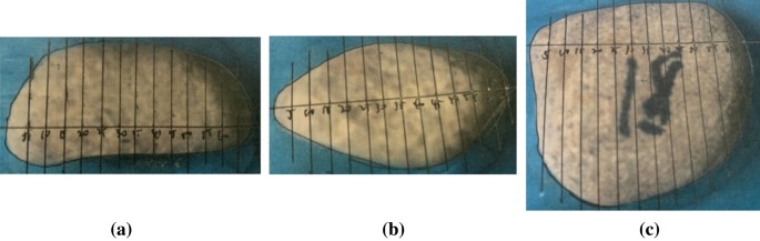
Three views: a the main view; b the left view; c the top view
- 2.
The lengths of the vertical lines were measured, and the data were exported to MATLAB. The results are shown in Fig. 4.
Fig. 4 
Three views: a the main view; b the left view; c the top view
- 3.
Combined with the polynomial algorithm, the 7th fit was selected, and the edge curves of the pebbles were fitted. The algorithm is shown in Eq. 1, and the coefficients for the three views are shown in Table 1.
$$ f(x) = p_{1} x^{7} + p_{2} x^{6} + p_{3} x^{5} + p_{4} x^{4} + p_{5} x^{3} + p_{6} x^{2} + p_{7} x^{1} + p_{8} $$(1)Table 1 Coefficients for the photographs The results are shown in Fig. 5.
Fig. 5 
Three views: a the main view; b the left view; c the top view
- 4.
The number of ball elements in the main view was first designed. Next, the major axes in the main view were separated into equal parts as the x-positions of the ball elements. The y-positions \( y \) and radius \( r \) of each ball element were calculated by Eqs. 2 and 3, respectively. Similarly, the left view was filled with separated ball elements. The results are shown in Fig. 6.
Fig. 6 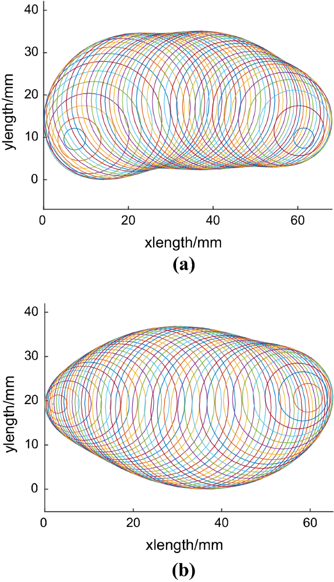
Ball elements filled in the main view and left view
$$ y = (y_{\text{up}} + y_{\text{down}} )/2 $$(2)$$ r = (y_{\text{up}} - y_{\text{down}} )/2 $$(3)where \( y_{\text{up}} \) is the y coordinate of the upper curve in the main view calculated by Eq. 1, and \( y_{\text{down}} \) is the y coordinate of the lower curve in the main view calculated by Eq. 1.
- 5.
Coupled with the ball element x-positions in the main view, the ball elements in the left view were extended to three dimensions, and the results are shown in Fig. 7a. Based on the edge curves of the main view, the ball element radius and z-positions were changed according to Eqs. 4 and 5, respectively, and the results are shown in Fig. 7b. Similarly, the ball element y-positions were recalculated according to the edge curves of the top view. The results are shown in Fig. 7c. Compared with a real pebble (Fig. 7d), the results indicate that this method can simulate the edge curves of a real pebble well.
$$ r_{\text{main}} = (z_{\text{up}} - z_{\text{down}} )/2 $$(4)$$ z_{\text{main}} = (z_{\text{up}} + z_{\text{down}} )/2 $$(5)where \( z_{\text{up}} \) is the z coordinate of the upper curve in the main view calculated by Eq. 1 and \( z_{\text{down}} \) is the z coordinate of the lower curve in the main view calculated by Eq. 1.
Fig. 7 
Pebble shape reconstruction process


In this paper, the number of ball elements was judged by the number of circles in the main view and the left view. The number of circles in the main view \( n_{\text{main}} \) was determined by the computational amount as well as the calculation accuracy. Next, the number of circles in the left view \( n_{\text{left}} \) was calculated by Eq. 4. Figure 8 shows the results with the number of circles in the main view as 3, 5, 10, and 15.
where \( l \) is the pebble length and \( w \) is the pebble width.

Results for different numbers of circles in the main view
3 Three-dimensional DEM simulation of the compression test system
3.1 The compression test system
This paper selected dynamic compression tests to calibrate the pebble DEM model. The compression test system is shown in Fig. 9, and the key technical parameters of the test system are given in Table 2.

Compression test system
In the experiment, the number of the tested pebbles was mainly judged by the computational amount as well as the calculation accuracy. With an increase in the number of pebbles, the computational amount correspondingly increases. It is impossible to simulate the procedure with a very large number of pebbles. However, the results may fluctuate if the number of tested pebbles is not enough. In this paper, the selected box size was measured as 0.343 m*0.236 m*0.1635 m, and the laying depth was preset to around 0.08 m.
The compression tests include three steps. First, the tested pebbles were placed into the box until the pebble thickness reached a preset value. Second, vertical speed was applied to the pressing plate, and the plate reached near the pebble horizontal surface. Third, a constant vertical velocity of 200 mm/min is applied to the pressing plate until the vertical displacement reached a preset depth. The compression process is shown in Fig. 10. In the testing process, signals of the pressing plate contacting forces and vertical displacements were recorded.

Compression process
At a pressing plate speed of 200 mm/min and pebble laying thickness of 0.0885 m, repetition test results of the compressing plate velocity were compared. The porosity was measured as 0.37, and the results are shown in Fig. 11.

Repetition test results
The results of the repetition tests show that with an increase in the pressing plate displacement, the contacting forces on the pressing plate increase considerably. Within 6.5 mm, the contacting forces increase linearly to about 1355 N. In addition, although there are some burrs in the displacement–force curves, the trend of these forces is roughly the same. The results indicate that the tested box size and the number of pebbles can be used for a calibration method for the pebbles used in truck escape ramps.
3.2 DEM simulation of the compression test system
-
1.
DEM algorithm
The DEM is mostly used for the mechanisms of element movement and interaction. The basic elements are the “ball” and “wall”. During the simulation process, the element interactions are judged by the positions of the elements, and the interactions are separated into “ball–ball” and “ball–wall.” If the elements are judged to be contacted, then a force–displacement law based on the Newton’s second law is established. The contacting mechanism is shown in Fig. 12, and the parameters are calculated by Eqs. 1–4 [33, 34].
where \( d \) is the “ball–ball” or “ball–wall” distance; \( x_{1} \) and \( x_{2} \) are the ball element coordinates; \( x_{3} \) is the point on the wall element that is nearest to the ball element; \( x_{4} \) is the middle point between the elements; \( n \) is the unit normal vector of the “ball–ball” or “ball–wall”; and \( c \) is the judging variable. When \( c \) is less than the minimum distance variable \( g_{c} \), the elements are judged to be contacted.

Element contacting mechanism: a ball–ball; b ball–wall
This paper selected the linear model as the “ball–ball” or “ball–wall” force–displacement contacting model. The linear model is separated into linear and damping parts. The linear part consists of elastic and friction force. The damping part consists of shear and normal damping force. The simplified contacting model is shown in Fig. 13.

Simplified contacting model
The elastic force is separated into normal elastic force \( F_{n}^{l} \) and shear elastic force \( F_{s}^{l} \) as follows:
where \( k_{n} \) is the normal stiffness, \( \frac{1}{{k_{n} }} = \frac{1}{{k_{n1} }} + \frac{1}{{k_{n2} }} \), where \( k_{n1} \) and \( k_{n2} \) are the normal stiffnesses of the ball or wall elements; \( \delta_{n} \) is the normal displacement of the elements; \( \left( {F_{s}^{l} } \right)_{0} \) is the linear shear force at the beginning of the timestep; \( k_{s} \) is the shear stiffness, \( \frac{1}{{k_{s} }} = \frac{1}{{k_{s1} }} + \frac{1}{{k_{s2} }} \), where \( k_{s1} \) and \( k_{s2} \) are the shear stiffnesses of the ball or wall elements; and \( \Delta \delta_{s} \) is the relative shear displacement of the elements.
When the shear elastic force is larger than the friction force, the shear elastic force is set to zero and the elements are only affected by the friction force \( F_{s}^{\mu } \):
where \( f_{s} \) is the friction coefficient. The friction coefficient is the minimum friction coefficient of the contacted elements.
The contacting elements are also affected by the damping force. Each time that two elements contact, part of the kinetic energy transforms into thermal energy. The local damping is imported into the DEM to restrict the relative motion. The damping force is proportional to the unbalanced force, and the force direction is opposite to the generalized velocity. The motion is transformed into the formula below:
where \( F_{i} \) is the unbalanced force; \( F_{i}^{d} \) is the damping force; \( M_{i} \) is the mass; and \( A_{i} \) is the acceleration.
where \( \alpha \) is the damping coefficient and \( v_{i} \) is the generalized velocity.
- 2.
DEM simulation process
The pebble DEM models were created using the proposed pebble shape construction method. We randomly built 50 pebble DEM model samples, and the results are shown in Fig. 14.

Pebble DEM model
The pebble DEM models were placed into a box DEM model using the “rainfall methods.” First, the pebbles were placed with equal spacing of 30 mm. The pebble sizes and the pebble rotations were randomly selected by the “rand” command. The results are shown in Fig. 15a. By the “gravity” command, the pebble DEM models were dropped into a box DEM model, and the processes are shown in Fig. 15a–c. By the “clump del” command, the pebbles with a preset laying thickness were settled. In this paper, the laying thickness was set to 0.0885 m, and the results are shown in Fig. 15d.

Simulation process
Then, a pressing plate DEM model was built by the “wall create” command. The plate was placed near the pebble surface. With an initial speed of 0.0333 m/s, the plate started to press into the pebbles. The evolutions of the contact force chain and pebble velocity during the simulation are shown in Figs. 16 and 17.

Evolution of the contact force chain

Evolution of the pebble velocity
4 The calibration of the pebble microscopic parameters
Based on the three-dimensional DEM model of the compression test system, the key parameter of the pebble DEM model friction coefficient was calibrated. In the simulation process, the element number and porosity were measured as 81,307 and 0.3732. The shear and normal stiffness were set to 2.4e7 N/m and 4.8e6 N/m [35]. The pebble density was measured as 2777 kg/m3. The results for different friction coefficients are shown in Fig. 18.

Results for different friction coefficients
The results show that at a laying thickness of 0.0885 m, the pressing plate contacting forces can be divided into two stages. The first stage is from 0 to 0.9255 mm. For friction coefficients of 0.2, 0.3, 0.4, 0.5, and 0.6, the contacting forces of the pressing plate increase to 5.737 N, 21.11 N, 63.55 N, 153.2 N, and 301.2 N, respectively. The second stage is from 0.9255 to 4.2 mm, and the compression forces increase to 70.35 N, 238.2 N, 604.5 N, 1837 N, and 4224 N, respectively. The results indicate that the basic trends of the simulation results are linearly shaped. The curves can be separated into two sections, and the forces in the second stage increase much more sharply than those in the first stage. The reason is that in the first stage, the pressing plate starts to press into the pebbles and the force deviations of different compressing velocities are not large. When the displacement reaches a certain degree, the function of the laying thickness becomes much more important and the contacting forces increase considerably. The results indicate that the friction coefficients greatly affect the simulation results. With an increase in the friction coefficients, the compression forces correspondingly increase.
Based on the compression test results, the friction coefficient was calibrated as 0.4. Simulation results and test results are compared. The results are shown in Fig. 19.

Comparison of the simulation and testing results
The results show that within 4.2 mm, the compression forces for the testing results and the simulation results increase to 587.4 N and 604.5 N, respectively. The results indicate that although there were some deviations, the trends of the simulation results are consistent with those of the experimental results. The results verified the feasibility of the simulation results. The errors in the simulation results mainly lie in the following aspects: The first method is the pebble shape calculation method. Considering the calculation amount, the pebble DEM model surface is not as flat as that of the real pebbles. The second aspect lies in the calibrated parameters; although the simulation results are consistent with the test results, the pebble DEM model parameters require further analysis.
5 The results for different pressing plate velocities and laying thicknesses
Based on the pebble DEM model parameters calibrated in previous chapters, the compression tests with different compressing plate velocities and laying thicknesses were simulated. During the simulation process, the signals from both the pressing plate displacement and contacting forces were recorded.
5.1 The simulation results of different pressing plate velocities
Based on the pebble DEM model parameters calibrated in previous chapters, compression tests were simulated with different pressing plate velocities. The pressing plate velocity was set by the “wall attribute velocity” command. This velocity was set as 3e−3 m/s, 4e−3 m/s, 5e−3 m/s, 6e−3 m/s, and 7e−3 m/s. During the simulation process, the thickness of the pebbles was set to 0.0885 m and the signals from both the pressing plate displacement and contacting forces were recorded. The results are shown in Fig. 20.

Results for different pressing plate velocities
The results show that within 4 mm, for pressing plate velocities of 3e−3 m/s, 4e−3 m/s, 5e−3 m/s, 6e−3 m/s, and 7e−3 m/s, the contacting forces increase to 625.5 N, 709.7 N, 851.2 N, 983.8 N, and 1003 N, respectively. The results indicate that the contacting forces of the pressing plate are linearly shaped, and for increases in the pressing plate velocity, the contacting forces correspondingly increase.
5.2 The simulation results for different laying thicknesses
Then, simulations were conducted with different laying thicknesses. The laying thicknesses were set as 0.045 m, 0.055 m, and 0.065 m. During the simulation process, the pressing plate velocity was set to 200 mm/min, and the signals from both the pressing plate displacement and contacting forces were recorded. The results are shown in Fig. 21.

Results for different laying thicknesses
The results show that within 3.5 mm, for laying thickness of 0.045 m, 0.055 m, and 0.065 m, the contacting forces increase to 398.9 N, 537.0 N, and 709.0 N, respectively. The results indicate that for increases in the laying thickness, the contacting forces on the pressing plate correspondingly decrease, and the contacting forces of the pressing plate are linearly shaped.
6 Discussion and conclusion
The main aim of this study is to find a proper way to simulate the irregularly shaped pebbles used in truck escape ramps. Coupled with the discrete element method (DEM) algorithm, this paper proposed a pebble DEM model to analyze the micro-contact mechanism of the pebbles. First is the pebble shape reconstruction method. Considering the computational amount and the calculation accuracy, the clumps with the overlapping method are the best choice. Coupled with a polynomial algorithm, this paper proposed a mathematical method to reconstruct the basic shapes of irregularly shaped pebbles. The results indicate that the proposed method is appropriate for reconstructing the rounded pebbles used in truck escape ramps. Second is the micro-parameters of the pebble DEM model. To calibrate the friction coefficient of the pebble DEM model, compression tests were conducted. The results verified the feasibility of the simulation method.
Next, compression tests were simulated with different plate velocities and laying thicknesses. The results for different compressing plate velocities indicate that the contacting forces of the plate are linearly shaped, and for increases in the compressing plate velocity, the contacting forces on the plate correspondingly increase. The results for different laying thicknesses indicate that for increases in the laying thickness, the contacting forces on the plate correspondingly decrease.
The shortcomings of this research mainly lie in the following aspects: First, the method is only suitable for rounded pebbles with smooth edge curves, and fractured pebbles with horizontal edge curves or sharp corners do not fit this method. Second, considering the computational amount, the shapes obtained from the pebble DEM models built in this paper were not as smooth as the real pebbles. Further studies will mainly concentrate on improving the calculation method and determining more precise pebble micro-parameters.
References
Abdelwahab W, Morral JF (1997) Determining need for and location of truck escape ramps. J Transp Eng 123(5):350–356
Wu KM, Hou DZ, Zhong LD, Li CC, Tang JJ (2014) Summary of and lessons from domestic and overseas setting of truck escape ramp. In: Applied mechanics and materials, 2014. Trans Tech Publications, pp 839–846
Pan BH, Liang RJ (2011) Research on the efflux angle to emergency escape ramp of mountain roads. In: Applied mechanics and materials. Trans Tech Publications, pp 257–265
Zhao X, Wang S, Yu M, Yu Q, Zhou C (2018) The position of speed bump in front of truck scale based on vehicle vibration performance. J Intell Fuzzy Syst 34(2):1083–1095
Al-Qadi IL, Rivera-Ortiz L (1991) Use of gravel properties to develop arrester bed stopping model. J Transp Eng 117(5):566–584
Horabik J, Parafiniuk P, Molenda M (2017) Discrete element modelling study of force distribution in a 3D pile of spherical particles. Powder Technol 312:194–203
Huang X, O’sullivan C, Hanley K, Kwok C (2014) Discrete-element method analysis of the state parameter. Geotechnique 64(12):954–965
Khanal M, Elmouttie M, Adhikary D (2017) Effects of particle shapes to achieve angle of repose and force displacement behaviour on granular assembly. Adv Powder Technol 28(8):1972–1976
Bonilla-Sierra V, Scholtes L, Donzé F, Elmouttie M (2015) Rock slope stability analysis using photogrammetric data and DFN–DEM modelling. Acta Geotech 10(4):497–511
Wang P, Arson C (2016) Discrete element modeling of shielding and size effects during single particle crushing. Comput Geotech 78:227–236
Jihong Y, Nian Q (2018) Combination of DEM/FEM for progressive collapse simulation of domes under earthquake action. Int J Steel Struct 18(1):305–316
Hazeghian M, Soroush A (2017) Numerical modeling of dip-slip faulting through granular soils using DEM. Soil Dyn Earthq Eng 97:155–171
Yang S, Zhang L, Luo K, Chew JW (2018) DEM investigation of the axial dispersion behavior of a binary mixture in the rotating drum. Powder Technol 330:93–104
André D, Levraut B, Tessier-Doyen N, Huger M (2017) A discrete element thermo-mechanical modelling of diffuse damage induced by thermal expansion mismatch of two-phase materials. Comput Methods Appl Mech Eng 318:898–916
Zhao C-L, Zang M-Y (2017) Application of the FEM/DEM and alternately moving road method to the simulation of tire-sand interactions. J Terrramech 72:27–38
Recuero A, Serban R, Peterson B, Sugiyama H, Jayakumar P, Negrut D (2017) A high-fidelity approach for vehicle mobility simulation: nonlinear finite element tires operating on granular material. J Terrramech 72:39–54
Johnson JB, Kulchitsky AV, Duvoy P, Iagnemma K, Senatore C, Arvidson RE, Moore J (2015) Discrete element method simulations of Mars Exploration Rover wheel performance. J Terrramech 62:31–40
Hang C, Gao X, Yuan M, Huang Y, Zhu R (2018) Discrete element simulations and experiments of soil disturbance as affected by the tine spacing of subsoiler. Biosys Eng 168:73–82
Zhang B, Regueiro R, Druckrey A, Alshibli K (2018) Construction of poly-ellipsoidal grain shapes from SMT imaging on sand, and the development of a new DEM contact detection algorithm. Eng Comput 35(2):733–771
Yan B, Regueiro RA (2019) Comparison between pure MPI and hybrid MPI-OpenMP parallelism for discrete element method (DEM) of ellipsoidal and poly-ellipsoidal particles. Comput Part Mech 6(2):271–295
Yan B, Regueiro RA (2018) A comprehensive study of MPI parallelism in three-dimensional discrete element method (DEM) simulation of complex-shaped granular particles. Comput Part Mech 5(4):553–577
Zhou W, Ma G, Chang X, Zhou C (2013) Influence of particle shape on behavior of rockfill using a three-dimensional deformable DEM. J Eng Mech 139(12):1868–1873
Govender N, Wilke DN, Wu C-Y, Rajamani R, Khinast J, Glasser BJ (2018) Large-scale GPU based DEM modeling of mixing using irregularly shaped particles. Adv Powder Technol 29(10):2476–2490
Wang B, Martin U, Rapp S (2017) Discrete element modeling of the single-particle crushing test for ballast stones. Comput Geotech 88:61–73
Fu R, Hu X, Zhou B (2017) Discrete element modeling of crushable sands considering realistic particle shape effect. Comput Geotech 91:179–191
Zhou W, Yang L, Ma G, Xu K, Lai Z, Chang X (2017) DEM modeling of shear bands in crushable and irregularly shaped granular materials. Granul Matter 19(2):25
Tong L, Wang YH (2015) DEM simulations of shear modulus and damping ratio of sand with emphasis on the effects of particle number, particle shape, and aging. Acta Geotech 10(1):117–130
Guo Y, Yang Y, Yu XB (2018) Influence of particle shape on the erodibility of non-cohesive soil: insights from coupled CFD–DEM simulations. Particuology 39:12–24
Falagush O, McDowell GR, Yu H-S (2015) Discrete element modeling of cone penetration tests incorporating particle shape and crushing. Int J Geomech 15(6):04015003
Coetzee C (2016) Calibration of the discrete element method and the effect of particle shape. Powder Technol 297:50–70
Zhao X, Liu P, Yu Q, Shi P, Ye Y (2019) On the effective speed control characteristics of a truck escape ramp based on the discrete element method. IEEE Access 7:80366–80379
Zeng Y, Jin L, Du X, Gao R (2015) Refined modeling and movement characteristics analyses of irregularly shaped particles. Int J Numer Anal Methods Geomech 39(4):388–408
Cundall PA (1971) A computer model for simulating progressive, large-scale movement in blocky rock system. In: Proceedings of the international symposium on rock mechanics
Cundall PA, Strack OD (1979) A discrete numerical model for granular assemblies. Geotechnique 29(1):47–65
Zhang G-Q, Sun C-X, Cheng X (2011) Determining method of arrested bed of truck escape ramp based on particle flow simulation. J High Transp Res Dev 28:118–123
Acknowledgements
This research is funded by the National Key R&D Program of China (2017YFC0803904), Key Research and Development Program of Shaanxi (2019ZDLGY15-02, 2018ZDCXL-GY-05-03-01), and the Youth Innovation Team of Shaanxi Universities.
Author information
Authors and Affiliations
Corresponding author
Ethics declarations
Conflict of interest
The authors declare that they have no conflict of interests.
Additional information
Publisher's Note
Springer Nature remains neutral with regard to jurisdictional claims in published maps and institutional affiliations.
Rights and permissions
About this article

Cite this article
Liu, P., Yu, Q., Zhao, X. et al. Three-dimensional discrete element modeling of the irregularly shaped pebbles used in a truck escape ramp. Comp. Part. Mech. 7, 479–490 (2020). https://doi.org/10.1007/s40571-019-00274-9
Received:
Revised:
Accepted:
Published:
Issue Date:
DOI: https://doi.org/10.1007/s40571-019-00274-9