
Abstract
The objective of the manuscript is to present an approach for analyzing the behavior of an industrial system under the cost free warranty policy. Under this policy, the various parameters of the system behavior under the working as well as the rest conditions are taken into the account. To increase the working efficiency and reduce the failure rate during and beyond warranty, the system goes under rest period after working a random amount of time. After taking complete rest, the system restarts again. Further, during the formulation, the failure and repair rates of the components of the systems are taken as a negative exponential distribution. A mathematical model of the system is developed based on the Markov process and hence the various parameters such as reliability, mean time to system failure, availability and expected profit are derived for a system. The effect of various parameters on to the system performance is analyzed. Finally, an illustrative example is taken for demonstrating the approach.
1 Introduction
Today’s with the growing complexities of the system day-to-day, system analyst or plant personnel always wants to manufacture the product with high-reliability in less time at lower cost. To achieve it, billions of dollars are being spent annually worldwide to develop reliable and efficient products. Further, the industry has always interested to find the failure component of the system which might affect product performance over time. However, failure is an inevitable fact related to products and systems. These failures may be the result of human error, poor maintenance, or inadequate testing and inspection. To improve the system reliability and availability, implementation of appropriate maintenance strategies play an important role. High performance of these units can be achieved with highly reliable subunits and perfect maintenance. To this effect the knowledge of behavior of system, their component(s) is customary to plan and adapt suitable maintenance strategies [8]. Therefore, in recent years, the importance of reliability theory has been increasing greatly with the innovation of recent technology for the purpose of making good products with high quality and designing highly reliable systems. To achieve it, a variety of methods exists in the literature for failure analysis which includes reliability block diagrams, Markov Modeling, failure mode and effect analysis, Petri nets, fault tree analysis, and so forth [1, 3, 5, 7].
In most of the existing studies, researchers have utilized the constant repair and failure rate after initial burn-in period of bath tub curve for repairable mechanical systems. For instance, Srinivasan and Gopalan [32] probabilistically analyzed a two unit system in which one unit is switched on and the other is put in cold standby. Venkatachalam [34] presented the reliability and availability of two units hot standby system by considering that hot standby is subject to the same rules as the basic unit. To study the effect of preventive maintenance (PM) on system performance, Mahmoud [25] discussed the cost–benefit analysis of a two unit cold standby redundant system with two types of failure and preventive maintenance. Shigeru and Masafumi [36] evaluated the availability of a parallel system with PM. Rander et al. [31] examined cost analysis of a two dissimilar cold standby system with preventive maintenance and replacement of standby. Gopalan and Bhanu [16] discussed the cost analysis of a two unit repairable system subject to on-line PM or repair. Srinivasan and Subramanian [33] improved the state of art of modeling and analysis with multiple units’ warm standby systems. Garg and Sharma [14] developed a two-phase approach for reliability and maintainability analysis of an industrial system. Lapa et al. [22] presented a methodology for PM policy evaluation based upon a cost-reliability model using a genetic algorithm. Leou [23] proposed a formulation considering both reliability and cost reduction for maintenance scheduling. Garg et al. [11] presented the PM scheduling for analyzing the behavior of the industrial systems. Garg and Sharma [12, 13] analyzed the behavior of the industrial system through various reliability parameters. Garg et al. [15] analyzed the behavior of the pulping unit of the paper industry by considering the time varying components of the failure rate and repair time. Apart from these, in the literature, numerous attempt have been made by the researchers to analyze the reliability of the system using different approaches [4, 6, 9, 10, 18,19,20,21, 24, 30, 35].
It is evident from the above-mentioned studies that all these models are analyzed without considering the concept of failure free warranty policy. As customers need assurance that the product they are buying will perform satisfactorily and warranty may provide such assurance. Providing warranty to the system for a certain period of operation is one of the effective ways to ensure the reliability of a component (or system) [29]. Under these conditions, authors in [29], [28] discussed reliability models of a single-unit system with warranty and different repair policies. Alqahtani and Gupta [2] discuss the effects of the warranty policy for the remanufactured products. Mo et al. [26] presented a new warranty policy wherein the buyer invests in the PM cost within the product’s life cycle to reduce the losses from production downtime. Huang et al. [17] presented an approach with preventive maintenance with extended policy.
Since the above existing models are widely applicable in many different fields, but they have restricted under the conditions that the unit/component or a system can perform without any rest, i.e., the system does not need any rest before its failure. Therefore, the credibility of the system and their corresponding approaches are not being well defined. However, in practice, it is not possible for a component or system to perform continuously for a long time with the same efficiency. Continuous usage of the system may increase the failure rate as well as may reduce its working efficiency. In these situations, the system needs some rest after working a random amount of time. Thus, keeping the inspiration from this fact, we have investigated the problem to analyze the reliability and the profit of the system based on the cost free warranty policy where the working period followed by a rest period. Therefore, the objective of this work is to present an approach to solve a single-unit system model following the periods of working and rest with failure free warranty policy using Markov process. In it, during the warranty, the product is repaired free of cost to the users on failure but the users will have to repair the failed units at their own expenses beyond warranty. Further, the failure and repair rates of the system are assumed to be followed a negative exponential distribution. Based on these, a various expressions which depict the behavior of the system such as reliability of the system, mean time to system failure (MTSF), availability and profit are derived using Markov process. To substantiate the proposed approach, the effect of various parameters of the system is analyzed through the system reliability, and expected profit with an illustrative example.
The remainder of the paper is organized as follows. Section 2 gives the description of the system containing the assumptions of the model, state-specifications, and notations related to the proposed system model. Section 3 presents the model analysis in which different system performance measures are computed such as reliability of the system and MTSF. Section 4 shows the results and discussion with special cases containing availability of the system and profit analysis of the user. Finally, Sect. 5 conclude the paper.
2 Description of the system
The present study for investigating the performance of industrial systems under the cost free warranty policy for a system whose failure and repair rates follows the negative exponential distribution. The following are the assumptions taken into account for modeling:
2.1 Assumptions
-
(i)
The system has a single-unit for operation.
-
(ii)
There is a single repair repairman who is always available with the system.
-
(iii)
The system has a working period followed by a rest period.
-
(iv)
All the repairs are cost free to the users during warranty, provided failures are not due to the negligence of users.
-
(v)
During warranty, the repairman inspects the failed unit to check whether the system is under warranty or not.
-
(vi)
During rest period no unit can fail, but a failed unit can be repaired.
-
(vii)
The unit works as new after its repair.
-
(viii)
The distribution of failure and repair time is taken as negative exponential.
2.2 State-specification
- S0/S7::
-
The unit is operative during working period within/beyond warranty.
- S1/S8::
-
The system is under rest period within/beyond warranty.
- S2::
-
The failed unit is under inspection to check whether the system is under warranty or not.
- S3/S5::
-
The failed unit is under repair during working period within/beyond warranty.
- S4/S6::
-
The failed unit is under repair during rest period within/beyond warranty.
2.3 Notations
- λ::
-
Constant failure rate of the unit within and beyond warranty.
- μ::
-
Constant repair rate of the unit within and beyond warranty.
- a::
-
Transition rate with which the working system goes under rest periods.
- b::
-
Transition rate with which the system goes from rest periods to working condition.
- p/q::
-
Probability that warranty is completed/not completed.
- h::
-
Constant inspection rate of the failed unit.
- p0(t)/p7(t)::
-
Probability density that at time t, the system is in state S i , i = 0, 7 and in good state within/beyond warranty.
- p1(t)/p8(t)::
-
Probability density that at time t, the system is in state S i , i = 1, 8 and in rest condition within/beyond warranty.
- p2(t)::
-
Probability density that at time t, the system is in state s2 and the unit is under inspection to check whether the system is under warranty or not.
- p3(t)/p5(t)::
-
Probability density that at time t, the system is in failed state S i , i = 3, 5 and the unit is under repair during working period within/beyond warranty.
- p4(t)/p6(t)::
-
Probability density that at time t, the system is in failed state S i , i = 4, 6 and the unit is under repair during rest period within/beyond warranty.
- p(s)::
-
Laplace transform of function p(t).
3 Model analysis
The system model consists of a single-unit in which there is a single repairman who always remains with the system and monitoring its performance. Consider that at initially, the unit is operative during the working period within warranty and when it is failed within warranty then it goes for inspection to check whether the unit is failed due to the negligence of the users or not. If it failed due to the negligence of the users then system warranty is completed and all the charges of repairs are borne by the users otherwise the failed unit is repaired cost free to the users during working periods. On the other hand, the unit goes under rest period after working a random amount of time and after taking complete rest, the system restarts again. During rest period no unit can fail, but a failed unit can be repaired. Assume that the failure and repair rates of the system follow a negative exponential distribution. Based on the assumptions and the notation, the transition diagram of this system by considering all the states, namely up (i.e., good or working) and failed states is shown in Fig. 1.

State-transition diagram of the system
3.1 Formulation of mathematical model
Based on this diagram, we can formulate the difference-differential equations using the probabilistic arguments of each state of the system and are summarized as follows
Initial conditions
Taking Laplace transform of all the above equations
From Eq. (13), we get
where
From Eq. (15), we get
where
From Eq. (14), we get
where
Using Eqs. (24) in (22),we get
From Eq. (12), we get
where
From Eq. (11), we get
where
From Eq. (17), we get
From Eq. (19), we get
Using Eqs. (32) in (18), we get
where
Now, using Eqs. (20), (33) and (31) in (16), we get
where
Using Eqs. (35) in (31), we get
Using Eqs. (35) in (33), we get
Now, using Eqs. (37) and (38) in (32), we get
where
It is worth noticing that
3.2 Evaluation of Laplace transform of up and down state probabilities
The Laplace transforms of probabilities that the system is in up state Pup(t) (i.e., good state) and down state Pdown(t) (i.e., failed state) at time ‘t’ are as follows
3.3 Reliability of the system
Reliability, R(t) of a system or product is the probability that the system or product functions well in a specified period of time. Using the method similar to that in Sect. 3.1, the difference-differential equations for reliability are [3]:
Taking Laplace transform of Eqs. (44) and (45) and using the initial conditions, we get
From Eq. (47), we get
Using Eqs. (48) in (46), we get
Equation (48) becomes as
Now, R(s) = p0(s) + p1(s).
Using Eqs. (49) and (50) and after solving, we get
Taking inverse Laplace transform of Eq. (51), we get
where
3.4 Mean time to system failure (MTSF)
MTSF is defined as the expected time for which the system is in operation before it completely fails.
Using Eq. (52) and after solving, we get
4 Results and discussion
In this section, the availability and the profit analysis of the system has been investigated through different parameters of the system.
4.1 Availability of the system
Availability, Av(t) of a repairable system is the probability that the system is operating satisfactorily at a specified time ‘t’. Using Eqs. (29) and (38), the Laplace transforms of Av(t) at time t is as follows
where
Taking Laplace transform of Eq. (55), we get
where
4.2 Profit analysis of the user
Availability of the system leads to the revenue, whereas the busy period of the repairman, number of repairs, etc., leads to the cost of maintenance. Therefore, profit analysis is an important aspect in the field of reliability and depends upon production cost of maintenance, failure rates, repairman employed, accidents, etc.
The revenue and cost function leads to the profit function of a firm, as the profit is excess of revenue over the cost of production. The profit function takes the form
Let us consider a system which involves the costs, K1 = revenue per unit up time of the system, K2 = repair cost per unit time and Av(t) = the total fraction of time for which the system is up. Then the expected profit is given by
Suppose that the warranty period of the system is (0, w]. Since the repairman is always available with the system, therefore, beyond warranty period, it remains busy for time (t − w) during the interval (w, t]. Then the expected profit H(t) during the interval (0, t] is given by
Using Eq. (56) and after solving, we get
Next, we have analyzed the performance of the system with respect to the various affecting parameters of the system which affects the system performance directly or indirectly. For it, the effect of the parameters, namely failure rate (λ), transition rate by which system goes under rest period (a) and repair cost (K2), on to the system reliability and the expected profit have been deducted. The results corresponding to these are summarized in Tables 1 and 2, respectively, for the reliability and the expected profit.
However, to analyze the effect of the individual components on the system reliability, an analysis has been conducted by varying each parameter at a times and simultaneously fixing the other parameters. The descriptions of these analyses have been summarized as follows:
-
(i)
If we increase the failure rate of the system within warranty, i.e., λ and fixing the other values, then their corresponding reliability of the system is decreased. For instance, if we increase λ from 0.1 to 0.2 then the reliability of the system at a particular time, say 5 units, is decreased by 26.98%. Similarly, if we further increase failure rate from 0.2 to 0.3, then their corresponding decrease occurs 25.67%. The complete variations of the effect of λ on the system reliability with the passage of the time are summarized in Fig. 2a.
Fig. 2 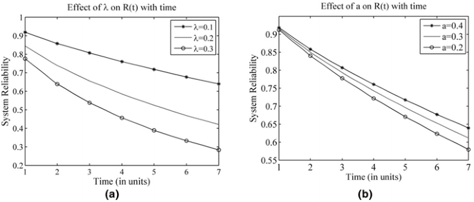
Effect of ‘λ’ and ‘a’ on system reliability
-
(ii)
Similarly, if we analyze the effect of the parameter (a) on the system reliability by preserving the other values then their impact on it has been computed and summarized in Fig. 2b for different values of the passage of time. From this figure, it has been concluded that whenever the value of (a) changes from 0.4 to 0.3 then further to 0.2, then the reliability of the system decreases with the passage of time from 0.71784 to 0.69625 and then further to 0.671146 for the time 5 units.

On the other hand, if we analyze the effect of the various parameters on to the expected profit H(t) during the interval (0, t] as given in Eq. (57). For it, firstly, we fix the different parameters as λ = 0.1, a = 0.4, b = 0.6, μ = 0.7, h = 0.9, p = q = 0.5, K1 = 1000. Now, the effect of the parameters namely repair cost (K2) and transition rate with which the working system goes under rest periods (a) conducted an experiment in which the values of these parameters on H(t) have been analyzed by fixing the values of the other component simultaneously with the passage of the time. The results corresponding to it have been summarized in Fig. 3. From this figure, we observed that if we decrease the repair cost, i.e., K2 from 200 to 150 and further to 100 and simultaneously fixing the other values, then their corresponding expected profit H(t) is first increases from 1 to 3 units and then decreases with respect to it. The complete variations of the effect of K2 on the expected profit with the passage of the time are summarized in Fig. 3a. On the other hand, the effect of the parameter a on to the expected profit H(t) by preserving the other values have been analyzed with the passage of the time. The variations of the expected profit with it have been summarized in Fig. 3b which depicts that by decreasing the parameter a from 0.4 to 0.3 and then further to 0.2, the expected profit will increase with the passage of the time. Thus, the different parameters have shown their effect on it, which will be beneficial for the system/reliability analyst to increasing the productivity of the system by adopting the necessary actions.

Effect of K2 and ‘a’ on to the expected profit
5 Conclusion
In the present paper, we have proposed an approach for analyzing the system reliability and profit with warranty policy. In it, the product is repaired free of cost to the users on failure during the warranty. The failure rate of the component of a system is considered to be followed by negative exponential distribution. The effect of the warranty as well as the failure component of the system on to the behavior of the system is analyzed by varying the different parameter of the system. From the analysis, it is found that by varying the parameters K2 and a, expected profit is increased and hence decision maker or system analyst may choose the appropriate values of these parameters according to their desired target, so as to increase the performance and productivity of the system. As compared to the existing model proposed by Kadyan and Niwas [20], when we set a = b = 0, i.e., when the system not goes for rest, failure as well as repair rates are not same within/beyond warranty and warranty is completed by a constant rate (α) not by doing the inspection of the failed unit, then the proposed model reduced to Kadyan and Niwas [20]. Additionally, it is observed that when there is no cost free warranty provided and by considering a 2-unit parallel system irrespective of single-unit system then the current model reduces to Murari and Muruthachalam [27] model. Thus, it is clearly seen that the proposed model is an extension of these existing model. Therefore, the present study reveals that after getting some rest during working a random amount of time within/beyond warranty, a system in which unit works as a new after its repair will be economically beneficial to use. So, our studying model is more reasonable and advance than the existing models. In the future, our research will look at the reliability and profit analysis for two or more unit systems and for the complex repairable industrial systems.
References
Adamyan A, David H (2002) Analysis of sequential failure for assessment of reliability and safety of manufacturing systems. Reliab Eng Syst Saf 76(3):227–236
Alqahtani AY, Gupta SM (2017) Warranty as a marketing strategy for remanufactured products. J Clean Prod 161:1294–1307
Ebeling C (2001) An introduction to reliability and maintainability engineering. Tata McGraw-Hill Company Ltd., New York
Garg H (2013) Performance analysis of reparable industrial systems using PSO and fuzzy confidence interval based methodology. ISA Trans 52(2):171–183
Garg H (2013) Reliability analysis of repairable systems using Petri nets and Vague Lambda-Tau methodology. ISA Trans 52(1):6–18
Garg H (2014) Performance and behavior analysis of repairable industrial systems using vague lambda-tau methodology. Appl Soft Comput 22:323–338
Garg H (2014) Reliability, availability and maintainability analysis of industrial systems using PSO and fuzzy methodology. MAPAN J Metrol Soc India 29(2):115–129
Garg H (2017) Performance analysis of an industrial system using soft computing based hybridized technique. J Braz Soc Mech Sci Eng 39(4):1441–1451
Garg H, Rani M (2013) An approach for reliability analysis of industrial systems using PSO and IFS technique. ISA Trans 52(6):701–710
Garg H, Rani M, Sharma SP (2013) Predicting uncertain behavior of press unit in a paper industry using artificial bee colony and fuzzy Lambda-Tau methodology. Appl Soft Comput 13(4):1869–1881
Garg H, Rani M, Sharma SP (2013) Preventive maintenance scheduling of the pulping unit in a paper plant. Japan J Ind Appl Math 30(2):397–414
Garg H, Sharma SP (2012) Behavior analysis of synthesis unit in fertilizer plant. Int J Qual Reliab Manag 29(2):217–232
Garg H, Sharma SP (2012) Stochastic behavior analysis of industrial systems utilizing uncertain data. ISA Trans 51(6):752–762
Garg H, Sharma SP (2012) A two-phase approach for reliability and maintainability analysis of an industrial system. Int J Reliab Qual Saf Eng (IJRQSE) 19(3):19 (Article ID 1250,013)
Garg H, Sharma SP, Rani M (2013) Weibull fuzzy probability distribution for analysing the behaviour of pulping unit in a paper industry. Int J Ind Syst Eng 14(4):395–413
Gopalan M, Bhanu K (1995) Cost analysis of a two unit repairable system subject to on-line preventive maintenance and/or repair. Microelectron Reliab 35(2):251–258
Huang YS, Huang CD, Ho JW (2017) A customized two-dimensional extended warranty with preventive maintenance. Eur J Oper Res 257(3):971–978
Ramniwas, Kadyan MS, Kumar J (2013) Stochastic modelling of a single-unit repairable system with preventive maintenance under warranty. Int J Comput Appl 75(14):36–41
Kadyan MS (2013) Reliability and profit analysis of a single-unit system with preventive maintenance subject to maximum operation time. Eksploatacja i Niezawodnosc 15:176–181
Kadyan MS, Niwas R (2013) Cost benefit analysis of a single-unit system with warranty for repair. Appl Math Comput 223:346–353
Kumar J, Kadyan M, Malik S (2013) Profit analysis of a 2-out-of-2 redundant system with single standby and degradation of the units after repair. Int J Syst Assur Eng Manag 4(4):424–434
Lapa CMF, Pereira CM, Barros MPD (2006) A model for preventive maintenance planning by genetic algorithms based on cost and reliability. Reliab Eng Syst Saf 91:233–240
Leou R (2006) A method for unit maintenance scheduling considering reliability and operation expense. Electr Power Energy Syst 28:471–481
Liao GL (2012) Optimum policy for a production system with major repair and preventive maintenance. Appl Math Model 36(11):5408–5417
Mahmoud M (1989) Reliability study of a two-unit cold standby redundant system with two types of failure and preventive maintenance. Microelectron Reliab 29(6):1061–1068
Mo S, Zeng J, Xu W (2017) A new warranty policy based on a buyer’s preventive maintenance investment. Comput Ind Eng 111:433–444
Murari K, Maruthachalam C (1981) 2-unit parallel system with periods of working and rest. IEEE Trans Reliab 30(1):91
Niwas R, Kadyan M, Kumar J (2015) Probabilistic analysis of two reliability models of a single-unit system with preventive maintenance beyond warranty and degradation. Eksploatacja i Niezawodnosc 17(4):535–543
Niwas R, Kadyan M, Kumar J (2016) Mtsf (mean time to system failure) and profit analysis of a single-unit system with inspection for feasibility of repair beyond warranty. Int J Syst Assur Eng Manag 7(1):198–204
Ram M, Kumar A (2015) Performability analysis of a system under 1-out-of-2: G scheme with perfect reworking. J Braz Soc Mech Sci Eng 37(3):1029–1038
Rander M, Kumar S, Kumar A (1994) Cost analysis of a two dissimilar cold standby system with preventive maintenance and replacement of standby. Microelectron Reliab 34(1):171–174
Srinivasan S, Gopalan M (1973) Probabilistic analysis of a 2-unit cold-standby system with a single repair facility. IEEE Trans Reliab 22(5):250–254
Srinivasan SK, Subramanian R (2006) Reliability analysis of a three unit warm standby redundant system with repair. Ann Oper Res 143(1):227
Venkatachalam P (1978) Stochastic behaviour of a 1-server 2-unit hot standby system. Microelectron Reliab 17(6):603–604
Wang W, Zhao F, Peng R (2014) A preventive maintenance model with a two-level inspection policy based on a three-stage failure process. Reliab Eng Syst Saf 121:207–220
Yanagi S, Sasaki M (1992) Availability of a parallel redundant system with preventive maintenance and common-cause failures. IEICE Trans Fundam Electron Commun Comput Sci 75(1):92–97
Acknowledgements
The second author (Harish Garg) would like to thanks the Thapar Institute of Engineering and Technology (Deemed University) Patiala for providing the financial support under SEED Money Grant wide letter no. TU/DORSP/57/1910.
Author information
Authors and Affiliations
Corresponding author
Additional information
Technical Editor: Fernando Antonio Forcellini.
Rights and permissions
About this article

Cite this article
Niwas, R., Garg, H. An approach for analyzing the reliability and profit of an industrial system based on the cost free warranty policy. J Braz. Soc. Mech. Sci. Eng. 40, 265 (2018). https://doi.org/10.1007/s40430-018-1167-8
Received:
Accepted:
Published:
DOI: https://doi.org/10.1007/s40430-018-1167-8