
Abstract
Harmonic drives are the core components to enable movement in industrial robots. Unfortunately, the deformation of flexspline causes obvious partial axial load on gear engagement. This synthetic error leads to a series of additional problems, such as the deterioration of transmission quality, and the reduction of both precision and fatigue life. This study focuses on a harmonic drive with a double circular-arc tooth profile. A coordinate transformation is carried out based on the kinematics of harmonic drives. On this basis, the conjugate tooth profile of a circular spline is derived. A simulation model is developed based on the motion relationship for harmonic transmission. The effect of inhomogeneity of the load distribution on the surface of the gear teeth was investigated using the partial axial-load index. The effect of different factors on the partial axial load is analyzed. To reduce the effect of partial axial load of flexspline, we select a suitable material and wall thickness. For a certain practical range, both tooth width and chamfering of the flexspline teeth help reduce the partial axial load and increase the flexspline length. These conclusions enable improvements of future designs of reliable flexspline.
1 Introduction
Due to their high transmission-ratio, high precision, compact structure, and coaxial input and output, harmonic drives are widely used for light-load joints of small and medium-sized robots. In other words, they are becoming an essential part of industrial robots [1, 2].
Harmonic drives consist of three components: circular spline, flexspline and wave generator. They enable the transfer of movement and power using a periodic spatial deformation of the flexspline. Because the wave generator is elliptical, or similar to an ellipse, when it rotates continuously, the shape of flexspline also changes. Furthermore, both deformation and rotation of flexspline also change the meshing state of the harmonic drive. Thus, a larger transmission ratio is obtained if there is a smaller number of teeth difference [3]. A harmonic drive is shown in Fig. 1.

Harmonic drive process-diagram
Unfortunately, harmonic drives always had problems with operating lives and accuracy over time with flexspline. Harmonic drives rely on the periodic elastic deformation of the flexspline to transmit motion. This makes the motion relationship between flexspline and circular spline more complex than for a general transmission device. Under normal circumstances, the design life of harmonic drives should be at least 8000–10,000 h. Harsh working conditions, the need for a long operating-life, and high accuracy are great challenges for the design and manufacturing of flexspline. For a periodic rotation and load action of the wave generator, the flexspline produces a cone angle and distortion following large deformation. Because of manufacturing and assembly errors, there are significant axial loading and several transmission problems, such as higher stress concentration, nonlinear meshing, a reduction of meshing stiffness, increasing transmission errors, and deterioration of transmission quality. These problems substantially affect the accuracy maintenance, fatigue life as well as operating noise of flexspline.
For engineering applications, because of manufacturing and assembly errors, bearing-clearance and deformation, and torsional deformation of the gear itself, the ideal meshing frequently cannot be achieved. Manufacturing and assembly errors, bearing-clearance and deformation will lead to the deviation between the actual geometric center and the theoretical geometric center. And the torque applied on flexspline will make the teeth deflect in the circumferential direction, resulting in the uneven force on the teeth in the meshing range. This leads to unwanted phenomena such as partial load during the meshing process, which also reduce gear meshing quality. Chase [4] from Brigham Young University studied the partial load for spline coupling caused by the manufacturing error. The model considered factors such as hardness, partial load, and clearance, and the stress for the tooth pair was predicted. Li [5, 6] from Shimane University carried out a loading tooth contact analysis (LTCA) using a stress calculation and finite element method. Gonzalez et al. studied the effect of axial error on partial gear load, and how to improve contact stress and transmission error by modifying the dislocation compensation [7]. Considering the effect of geometric parameters, as well as the partial load, Liu et al. proposed a 10-DOF nonlinear dynamic model. The effect of different modification on the dynamic load were determined [8]. Using the theory of the concentrated parameter, Wu et al. used a nonlinear dynamic model for a ravigneaux compound planetary gear with an intermediate floating component. The effect of both assembly error and eccentricity error on the system load characteristics was analyzed. The analysis results indicate that the installation error for the planet gear caused the planets to experience a continuous “partial load”, while the eccentricity error for the planet gear endowed the corresponding meshing pairs with a greater impact during the movement [9, 10].
The occurrence of partial gear-load causes several problems such as non-linearity of the meshing, reduction of meshing stiffness, increase of transmission error, deterioration of transmission quality, and a reduction of the fatigue life. Tugan et al. believed that the non-linearity of gear meshing is due to contact loss in the gear meshing. A model which could describe the distribution of the contact force for any tooth surface, was introduced [11]. Matsumura et al. [12] analyzed the relationship between load distribution and mating surface deformation. They developed a numerical analysis-method for gear vibration, which can take any type of deviation into account. The vibration behavior of a pair of helical gears under partial load with tooth surface deviation was analyzed. The results show that when the transmission operates under light load, the contact mode of the gear pair does not cover the entire tooth surface, and the vibration response varies with the transmission load. Ghaffari [13, 14] used the damage mechanics method to simulate the cracks on the gear surface. The effect of friction on fatigue was investigated considering the partial load conditions. Wang [15, 16] used the lumped parameter method to analyze the contact of the spur gear pair. The impact of the assembly error on the gear drive dynamics was studied. Even if the assembly errors are assumed sufficiently small, they can lead to load concentration and deterioration of the gear transmission quality. Tang [17] established a gear-dynamics equation and analyzed the effects of modification, parallelism of the gear axis, and load on the dynamic response of gears using numerical solutions. A study by Wang shows that the key factor, which causes failure of wind turbine gearboxes, is caused by partial load rather than material defects [18]. Li [19] studied the partial load problem of a planetary gear train used in helicopters. The optimized design of the tooth profile is conducive to any improvement of partial load. Yuan [20] studied the effect of diagonal modification on the tooth surface load distribution, the overall meshing stiffness, and the bearing transfer error. Pacana [21] analyzed the stress of flexspline by theoretical calculation and simulation analysis, and carried out experimental verification to obtain the relationship between rotation angle and stress. Sahoo [22] established the evidence of secondary contacts and probable load shared by those contacts experimentally over the finite element analysis. Wang [23] studied the stress calculation methods for short flexspline, based on mechanics analysis and finite element method (FEM). The stress under different design parameters is analyzed to provide reference for design. Many researchers have been trying to improve the performance of harmonic drives by designing better tooth shapes or choosing more suitable materials [24,25,26,27,28,29,30,31,32].
To summarize, in the large field of harmonic drive research, recent studies always focused on a reduction of the impact of partial load using the lumped parameter method or modification of the tooth shape. Systematic analyses of the cause of partial load are not sufficient. The partial load of flexspline introduces several transmission problems such as short service life and insufficient accuracy. We explore the above problems by analyzing the structural and material choices that affect the partial load of flexspline.
2 Motion Geometry and Tooth-Profile Design
This paper focuses on a flexspline with a double-circular-arc tooth profile, which is widely considered to have better meshing quality [29, 33,34,35]. Based on the kinematics of the harmonic drive, a coordinate transformation was carried out. The tooth profile for the circular spline was derived using envelope theory.
2.1 Solution for the Flexspline Deformation
The relationship between the neutral layer original curve of flexspline and the wave generator is shown in Fig. 2.

Relationship between the neutral layer original curve of flexspline and wave generator
The wave generator is assumed a standard ellipse. It can be described using
The neutral layer original curve is actually a normal curve that is equidistant from the wave generator. The unit normal vector at any point can be written as
The parameters describing the flexspline motion geometry are shown in Table 1.
If the thickness of the flexible bearing is db, and the thickness of the cup body of the flexspline is df, then the neutral layer curve can be expressed as
Assuming:
Equation 3 can be rewritten as
Thus, the neutral layer curve can be expressed as
Combined with Eqs. (1), (5) can be rewritten as
After the wave generator was installed in the flexible bearing, the amount of radial deformation for the neutral layer can be expressed as
Then, the tangential displacement v and normal angle μ for any point on the neutral layer original curve can be obtained using Eq. (8) [36, 37].
2.2 Flexspline Tooth Profile Design
The tooth profile consists of two circular arcs (at the tooth face and at the tooth flank) and a straight line-segment. The straight line-segment near the index circle is the tangent of two circular arcs.
A dynamic coordinate-system (x1, o1, y1) is used with regard to the axial section of the flexspline tooth, where y1 is the symmetrical axis of the tooth and o1 is the intersection point between the neutral curve and the y1 axis. The variable parameters are shown in Fig. 3.

Definition of variable parameters for the flexspline tooth profile
According to the definition shown in Fig. 3, the tooth profile can be defined by Table 2.
We use the tooth-profile arc length s as an independent variable to describe the double arc profile function as follows:
-
1.
Tooth-flank arc segment (AB)—see Eq. (9)
$$\left\{ {\begin{array}{l} {X_{1} = R \cdot X_{\text{u}} + T} \\ {X_{\text{u}} = \rho_{\text{d}} \cdot R_{\text{u}} } \\ \end{array} } \right.\;s \in \left[ {0,l_{\text{AB}} } \right]$$(9)
where
-
2.
Straight line segment (BC)—see Eq. (10)
$$X_{1} = \left( {s - l_{\text{AB}} } \right)R_{\text{u}} + T\;\;s \in \left[ {l_{\text{AB}} ,l_{\text{AB}} + l_{\text{BC}} } \right]$$(10)
where
-
3.
Tooth-flank arc segment (CD)—see Eq. (11)
$$\left\{ {\begin{array}{l} {X_{1} = R \cdot X_{\text{u}} + T} \\ {X_{\text{u}} = \rho_{a} \cdot R_{\text{u}} } \\ \end{array} } \right.$$(11)
where
2.3 Motion Geometry of Harmonic Drive and Solution for the Tooth Profile
For the process of conjugate engagement, it is necessary to clarify the motion relationship.
By defining the vertical direction as the y2 axis, and the rotation center of circular spline as the origin o2, a fixed coordinate-system {x2, o2, y2} for the circular spline is established. Furthermore, by defining the rotation center of the wave generator as the origin o, a coordinate-system {x, o, y} for a circular spline is established—see Fig. 4.

Coordinate transformation relationship for a harmonic drive
Consistent with the principle of harmonic drives, the wave generator rotates counterclockwise. We now need to describe the tooth profile equation for a fixed coordinate system {x2, o2, y2}.
By analyzing the coordinate transformation, the transformation matrix from the coordinate system of flexspline {x1, o1, y1} to the coordinate system of circular spline {x2, o2, y2} can be expressed as
where Δφ is the angle between the meshing teeth of flexspline and the vertical direction. Mfc is the transformation matrix (Eq. 13) from {x1, o1, y1} to the coordinate system of circular spline {x2, o2, y2}.
After substituting the flexspline profile curve into Eq. (12), we can draw a series of curve families (see Eq. 13). Then, we use the envelope of these curve families as tooth profile for the circular spline (Fig. 5). Figure 5 describes the envelope process of flexspline and circular spline tooth profiles. The wave generator rotates counterclockwise, the tooth profile of flexspline rotates clockwise and then conjugates with the tooth top and tooth root arc of the circular spline.

Tooth profile for the circular spline using the envelope of the flexspline profile curve families
It can be seen that the circular spline and flexspline mesh very well during movement.
3 Geometric and Finite-Element Modeling
3.1 Geometric Modelling of Flexspline
The flexspline is a very thin-walled spur-gear, which is subjected to alternating loads during harmonic motion. This has a strong effect on the transmission accuracy and service life of the harmonic drive, and it is prone to fatigue damage.
In this paper we use a cup-type flexspline, which is modeled as shown in Fig. 6.

Geometric model of the flexspline
According to the definition in Fig. 6, the geometric model can be defined by Table 3.
3.2 Finite-Element Modelling
Three-dimensional elements are used for finite-element modelling. The structure is divided into two parts while generating mesh, the gear and the cup body. Mesh generation of the gear part and wave generator are accomplished by sweeping with the mesh type as hexahedron element (Solid 185). The mesh density is gradually refined in the tooth area, which represents the potential contact region. Tetrahedral element (Solid 187) is used in the cup body part. The finite model consists of 56,266 elements and is shown in Fig. 7.

Finite element model of flexspline and wave generator
The material settings used in the finite element model are shown as Table 4.
The the bottom of the flexspline and inner hole of the wave generator are fully restrained. The contact type of flexspline, wave generator and circular spline are represented by CONTAC185 in ANSYS. The applied torque between the circular spline and flexspline is 25 Nm.
The results indicate that the stress is concentrated at both ends of the teeth, especially at the back end of the teeth (Fig. 8).

Von-Mises stress in flexspline
It can be seen, that, when aided by the wave generator, the stress distribution at the root of the gear tooth is unevenly distributed in the direction of tooth thickness. Stress builds up at the front and back end of the teeth.
To verify the validity of the FEM model, we compared the simulation results with the calculated results using a Hertz contact model. Hertz contact theory is used to analyze strain and stress distribution of two objects during compressive contact. It uses three assumptions: (1) small deformation in the contact area; (2) elliptical contact area; (3) the contact object with distributed vertical pressure can be regarded as elastic half space. Because the width of the contact zone of the harmonic drive is much smaller than its curvature, Hertz contact theory can be used for stress analysis.
The meshing of circular spline and flexspline teeth can be equivalent to the contact of two instantaneous cylinders [38].
The maximum contact stress of two contact cylinders is
where E* is the composite material coefficient, ρ* is the composite curvature radius and
where μ1 and μ2 are Poisson ratios of the two cylinder materials, E1 and E2 are the elastic moduli of the two cylinder materials and
where ρ1 and ρ2 are the curvature radii associated with the two cylinders.
The normal load that corresponds to the equivalent elastic cylinders P is
where αt is the pressure angle for the end pitch circle, α ’t is the end engaging angle, K is the load coefficient, Ft is the tangential force, b is the tooth width, β is the helix angle and T is the transfer torque:
The curvature radii for the equivalent contact cylinders at the meshing point are:
where u is the gear ratio and β is the helix angle of the base circle.
Substituting the above equations into Eq. (14), we can get the equation for maximum contact stress:
We carried out a simulation of single tooth pairs (Fig. 9). The simulation process is as follows: (1) The circular spline and flexspline models of single tooth are established according to the involute profile; (2) In the FEM model, their material properties are taken according to Tab. 4. And the contacting zone of two gears is refined. The outer wall of circular spline is fixed, and the torque is applied through the inner wall of flexspline. (3) In the simulation process, the torque applied on the flexspline increases from 5 to 50 N m. Finally, the contact stress is extracted. The simulation results are compared with the calculated values using Hertz contact theory.

Meshing simulation of single tooth pair
A comparison between theoretical calculation and simulation is shown in Fig. 10.

The comparison between theoretical calculation and simulation
We can see that the maximum error between simulation and theory-based results is less than 10%, which means the model is quite accurate.
4 Results and Discussion
Subsequently, we focused on the circular spline and applied a torque of 10 N m.
The stress at the root of flexspline suggests the presence of partial load (Fig. 11). We then extracted the stress for the root of the ten meshing teeth in the meshing area. The simulation results are shown as Fig. 12.

Von-Mises stress of flexspline with circular spline and torque

Stress for the root of the ten meshing teeth in the meshing area
The results in Fig. 12 indicate that the stress value of 1th–4th teeth decreases, but that of 4th–10th teeth increases with the meshing process. The 4th tooth is the position with the smallest stress, which is due to the large meshing contact area and without the stress concentration. The value of stress fluctuates at the 9th and 10th teeth, which indicates that there exists the meshing impact at this position.
To study the effect of the structural parameters of flexspline on the partial axial load, we also conducted single-factor control simulations.
The circular spline and flexspline is engaged together by multiple tooth. The meshing state of gears mainly includes engaging-in, engaging and engaging-out. The partial load coefficient is considered in this paper, mainly since the stress of the different teeth with different engaging state while transferring the torque. The concept of partial axial load index is used to characterize the inhomogeneity of a load distribution on the mesh tooth surfaces. Taking σa as the average stress for a single tooth surface and σs as the standard deviation for the stress of the sampling points on the tooth surface, the bias load index P is defined as:
where i is the order of different teeth in the meshing area, and j is the stress extraction point for the tooth root.
In order to study the partial axial load index of different flexspline materials, the material 35CrMnSiA is taken as the control group. The detailed steps are as follows:
-
Step 1: The control group (Material 35CrMnSiA) is firstly studied. In the simulation model (Fig. 7), we take materials of the flexspline, circular spline and wave generator as 35CrMnSiA, 42CrMo and 45#, respectively. Their material properties are listed in Tab.4, including tensile modulus, poisson ratio, shear modulus, and density.
-
Step 2: The simulation analysis is performed based on definitions of the torque and boundary conditions. Then, the stress for the root of each meshing tooth in the meshing area is extracted.
-
Step 3: The partial axial load index of the material is obtained through substituting the extracted stress value into Eq. (22).
-
Step 4: The material of flexspline is replaced by 18Cr2Ni4WA (Level 1), 40Cr (Level 2) and QBe1.7 (Level 3) respectively. Then the partial axial load index under different materials can be obtained by repeating steps 1–3. The material settings for flexspline are shown in Table 5.
Table 5 Material settings for flexspline
The result for the partial axial load index are shown in Fig. 13.

Partial axial load index for different flexspline materials
Because there is little difference with regard to material properties of different steels, the corresponding partial load effect shows almost no difference. However, the special properties of QBe1.7 produce an increase of partial axial load.
Then, we compared the effect of the structural parameters of the flexspline body on the partial load.
-
1.
Wall thickness of flexspline tf
The values of the contrast parameters are shown in Table 6.
Table 6 Values of the contrast parameters-wall thickness of flexspline (mm) The result of partial axial load index is shown in Fig. 14.
Fig. 14 
Partial axial load index for different wall thicknesses of flexspline
-
2.
Length of flexspline (cup body) l1
The values of the contrast parameters are shown in Table 7.
Table 7 The values of the contrast parameters-lengths of flexspline (mm) The result for the partial axial load index is shown in Fig. 15.
Fig. 15 
Partial axial load index for different lengths of flexspline
-
3.
Teeth width lg
The values of the contrast parameters are shown in Table 8.
Table 8 Value of the contrast parameters teeth width (mm) The result of the partial axial load index is shown in Fig. 16.
Fig. 16 
Partial axial load index for different teeth widths of flexspline
-
4.
Chamfering of flexspline front end teeth θ1
The values of the contrast parameters are shown in Table 9.
Table 9 The values for contrast parameter chamfering of the flexspline front end teeth (°) The results for the partial axial load index are shown in Fig. 17.
Fig. 17 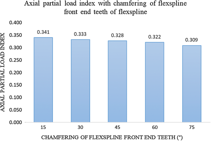
Partial axial load index for different chamfering of the flexspline front end teeth
-
5.
Chamfering of flexspline back end teeth θ2
The values of the contrast parameters are shown in Table 10.
Table 10 Values for contrast parameters chamfering of the flexspline back end teeth (°) The results for the partial axial load index are shown in Fig. 18.
Fig. 18 
Partial axial load index for different chamfering of flexspline back end teeth


Based on the above results, we can draw the following conclusion:
-
1.
Very thick or very thin walls of flexspline tf cause a deterioration of the partial axial load.
-
2.
The increase of the length of flexspline l1, the teeth width lg, the chamfering of flexspline front end teeth θ1 and the chamfering of flexspline back end teeth θ2 help reduce partial load. Especially the increase in chamfering of the flexspline back end teeth θ2 significantly reduces the partial axial load. For increasing length of flexspline l1 and tooth width lg, the improvement of partial axial load tends to be small.
By summarizing the above research, the final material and design parameters are shown in Table 11, considering the partial axial load index.
5 Conclusion
This study focuses on a harmonic drive with a double-circular-arc tooth profile. A coordinate transformation was carried out based on the kinematics and the tooth profile of the circular spline was derived. We established a simulation model based on the motion relationship for a harmonic transmission. The distribution inhomogeneity of load distribution on the surfaces of gear tooth by the concept of partial axial load index. The effect of different factors on partial axial load was analyzed. The analysis suggests that, to reduce the partial axial load of flexspline, it is necessary to select the correct material and wall thickness for flexspline. The teeth width and the chamfering of flexspline teeth help reduce the partial axial load and increase the length of flexspline.
References
Lee, S. D., & Song, J. B. (2016). Sensorless collision detection based on friction model for a robot manipulator. International Journal of Precision Engineering and Manufacturing,17(1), 11–17.
Kim, I. M., Kim, H. S., & Song, J. B. (2012). Design of joint torque sensor with reduced torque ripple for a robot manipulator. International Journal of Precision Engineering and Manufacturing,13(10), 1773–1779.
Pham, A. D., & Ahn, H. J. (2018). High precision reducers for industrial robots driving 4th industrial revolution: State of arts, analysis, design, performance evaluation and perspective. International Journal of Precision Engineering and Manufacturing-Green Technology,5(4), 519–533.
Chase, K. W., Sorensen, C. D., & Decaires, B. (2009). Variation analysis of tooth engagement and load-sharing in involute splines (pp. 219–232). American Gear Manufacturers Association Fall Technical Meeting.
Shuting, L. (2012). Contact stress and root stress analyses of thin-rimmed spur gears with inclined webs. Journal of Mechanical Design,119, 61–73.
Shuting, L. (2018). A mathematical model and numeric method for contact analysis of rolling bearings. Mechanism and Machine Theory,134, 1–13.
Gonzalez, P. I., Roda, C. V., & Fuentes, A. (2015). Modified geometry of spur gear drives for compensation of shaft deflections. Meccanica,50(7), 1855–1867.
Liu, H., Zhang, C., Xiang, C. L., & Wang, C. (2016). Tooth profile modification based on lateral-torsional-rocking coupled nonlinear dynamic model of gear system. Mechanism and Machine Theory,105, 606–619.
Wu, S. J., Peng, Z., Wang, X. S., Zhu, W. L., & Li, H. W. (2015). Impact of mesh errors on dynamic load sharing characteristics of compound planetary gear sets. Journal of Mechanical Engineering,51(3), 29–36.
Zhu, W. L., Wu, S. J., Wang, X. S., Zhou, L., Zhang, H. B., & He, R. (2016). Influence of position errors on the load-sharing characteristics of compound planetary gear sets considering the variable stiffness coefficient. Journal of Vibration and Shock,35(12), 77–85.
Eritenel, T., & Parker, R. G. (2012). An investigation of tooth mesh nonlinearity and partial contact loss in gear pairs using a lumped-parameter model. Mechanism and Machine Theory,56(1), 28–51.
Matsumura, S., Umezawa, K., & Houjoh, H. (1996). Rotational vibration of a helical gear pair having tooth surface deviation during transmission of light load. JSME International Journal Series C: Mechanical Systems Machine Elements and Manufacturing,39(3), 614–620.
Ghaffari, M. A., Pahl, E., & Xiao, S. (2015). Three dimensional fatigue crack initiation and propagation analysis of a gear tooth under various load conditions and fatigue life extension with boron/epoxy patches. Engineering Fracture Mechanics,135, 126–146.
Ghaffari, M. A., & Xiao, S. (2014). Fatigue crack propagation analysis of gear tooth under various load conditions and repaired with boron/epoxy patch. In ASME power conference (p. 9). Boston(US).
Wang, J., & Lim, T. C. (2015). Influence of assembly error and bearing elasticity on the dynamics of spur gear pair. ARCHIVE Proceedings of the Institution of Mechanical Engineers Part C Journal of Mechanical Engineering Science 1989–1996,203–210, 1805–1818.
Wang, J., Lim, T. C., & Yuan, L. (2013). Spur gear multi-tooth contact dynamics under the influence of bearing elasticity and assembly errors. Proceedings of Institution of Mechanical Engineers Part C Journal of Mechanical Engineering Science,227(11), 2440–2455.
Luo, C., Tang, J., & Chen, S. (2011). Influence of gear lead crown modification and misalignment on gear transmission characteristics. Mechanical Science & Technology for Aerospace Engineering,30(8), 1321–1331.
Wang, Q., Zhu, Y., Zhang, Z., Fu, C., Dong, C., & Su, H. (2015). Partial load: A key factor resulting in the failure of gear in the wind turbine gearbox. Journal of Failure Analysis and Prevention,16(1), 1–14.
Li, M., Xie, L., & Ding, L. (2017). Load sharing analysis and reliability prediction for planetary gear train of helicopter. Mechanism and Machine Theory,115, 97–113.
Yuan, B., Chang, S., Liu, G., Chang, L., & Liu, L. (2017). Optimization of bias modification and dynamic behavior analysis of helical gear system. Advances in Mechanical Engineering,9(11), 168781401773325.
Pacana, J., Witkowski, W., & Mucha, J. (2017). FEM analysis of stress distribution in the hermetic harmonic drive flexspline. Strength of Materials,49(1), 1–11.
Sahoo, V., & Maiti, R. (2018). Evidence of secondary tooth contact in harmonic drive, with involute toothed gear pair, through experimental and finite element analyses of stresses in flex-gear cup. Proceedings of the Institution of Mechanical Engineers, Part C: Journal of Mechanical Engineering Science,232(2), 341–357.
Wang, S., Jiang, G., & Mei, X. (2019). A rapid stress calculation method for short flexspline harmonic drive. Engineering Computations,36(6), 1852–1867.
Maiti, R. (2004). A novel harmonic drive with pure involute tooth gear pair. Journal of Mechanical Design,126(1), 178–182.
Krisch, R., & Házkötő, I. (2007). Investigation of the load transmission in the toothing of a flat wheel harmonic gear drive. Periodica Polytechnica Mechanical Engineering,52(2), 107–112.
Liu, Z., Zhang, T., Wang, Y., Yang, C., & Zhao, Y. (2019). Experimental studies on torsional stiffness of cycloid gear based on machining parameters of tooth surfaces. International Journal of Precision Engineering and Manufacturing,20(6), 1017–1025.
Dong, H., Wang, D., & Ting, K. L. (2011). Kinematic effect of the compliant cup in harmonic drives. Journal of Mechanical Design,133(5), 051004.
Dong, H., Ting, K. L., & Wang, D. (2011). Kinematic fundamentals of planar harmonic drives. Journal of Mechanical Design,133(1), 011007.
Chen, X., Liu, Y., Xing, J., Lin, S., & Xu, W. (2014). The parametric design of double-circular-arc tooth profile and its influence on the functional backlash of harmonic drive. Mechanism and Machine Theory,73(2), 1–24.
Ma, D. H., Wu, J. N., & Yan, S. Z. (2016). A method for detection and quantification of meshing characteristics of harmonic drive gears using computer vision. Science China,59(9), 1305–1319.
Zhang, C., Song, Z., Liu, Z., Yang, C., Cheng, Q., & Liu, M. (2018). Tribological properties of flexspline materials regulated by micro-metallographic structure. Tribology International,127, 177–186.
Ma, D. H., Wu, J. N., Liu, T., et al. (2017). Deformation analysis of the flexspline of harmonic drive gears considering the driving speed effect using laser sensors. Science China,8, 1–13.
Kiyosawa, Y., Sesahara, M., & Ishikawa, S. (1989). Performance of a strain wave gearing using a new tooth profile. In Proceedings, ASME international power transmission and gearing conference (pp. 607–612).
Ishikawa, S. (1989). Tooth profile of spline of strain wave gearing: US, US4823638.
Ishikawa, S., & Kiyosawa, Y. (1995). Flexing contact type gear drive of non-profile-shifted two-circular-arc composite tooth profile: US, US5458023.
Wang, J. X., Zhou, X. X., Li, J. Y., et al. (2016). Design of double-circular-arc and common tangent tooth profile of harmonic drive. Journal of Hunan University Natural Sciences,43(2), 56–63.
Wang, J. X., Zhou, X. X., Li, J. Y., et al. (2016). Three dimensional profile design of cup harmonic drive with double-circular-arc common-tangent tooth profile. Journal of Zhejiang University,50(4), 616–624.
Zhupanska, O. I. (2011). Contact problem for elastic spheres: Applicability of the Hertz theory to non-small contact areas. International Journal of Engineering Science,49(7), 576–588
Acknowledgement
This project is supported by National Natural Science Foundation of China (Grant No. 51805012), Natural Science Foundation of Beijing Municipality (CN) (Grant No. 3192003), and Beijing Municipal Education Commission (Grant No. KM201810005013).
Author information
Authors and Affiliations
Corresponding author
Ethics declarations
Conflicts of interest
The authors declare that they have no competing interests.
Additional information
Publisher's Note
Springer Nature remains neutral with regard to jurisdictional claims in published maps and institutional affiliations.
Rights and permissions
About this article

Cite this article
Yang, C., Hu, Q., Liu, Z. et al. Analysis of the Partial Axial Load of a Very Thin-Walled Spur-Gear (Flexspline) of a Harmonic Drive. Int. J. Precis. Eng. Manuf. 21, 1333–1345 (2020). https://doi.org/10.1007/s12541-020-00333-9
Received:
Revised:
Accepted:
Published:
Issue Date:
DOI: https://doi.org/10.1007/s12541-020-00333-9