
Abstract
In order to solve the analytical solution of the general rate-dependent model and make the theoretical model better reflect the creep behavior of soil, the fractional calculus theory is applied to the EVP (elastic–viscoplastic) model based on the overstress theory. A fractional strain rate model is proposed to construct a constitutive equation of fractional strain rate. The analytical solution of the fractional creep model is solved by applying Laplace integral transformation, and the fractional creep equation under undrained conditions is discussed. Then, the undrained shear creep test results of isotropic consolidated Fukakusa clay and K0 consolidated Sackville clay are used to verify the validity of the time-based fractional creep equation and the sensitivity analysis of the analytical solution. The effectiveness of the fractional creep model for predicting the creep behavior of soil such as soft clay is revealed. The results show that the fractional EVP creep model is obviously better than the traditional integer EVP model. Moreover, when the fractional order is 1, the fractional strain rate model can be reduced to an integer strain rate model, but the fractional creep equation degenerates into a linear creep equation.
1 Introduction
Soil is a kind of soft and loose porous medium. Its special structural characteristics and physical properties enable it to have certain creep characteristics. The uneven secondary compression is an important component in practical engineering to reduce the safety and durability of slope engineering and bridge engineering et al. [4, 32].
In recent years, a number of soil creep models have been proposed by researchers, such as empirical model, element model, and rate dependent model. Considering the prediction ability and model parameters of the model, the creep model based on the theory of EVP (elastic–viscoplastic) constitutive and overstress theories is highly recognized. Based on this, scholars have established many strain rate models describing soil creep [13]. Adachi [1] and Katona [11] established the creep model with certain prediction ability by cited the Cam-Clay yield model [19] and the modified Cam-Clay model proposed by Roscoe [20], respectively. Katona solved the implicit solution of the creep model through displacement finite element analysis and Newten–Raphson iteration theory. Hinchberger and Rowe [9, 10, 21] combined the EVP model and Biot consolidation theory to describe the non-structural creep response of clay using Druck–Prager failure envelope and critical state theory. The creep model with the Cam-Clay model and the modified Cam-Clay model as the dynamic yield surface was compared and analyzed. The conclusion that the latter is better than the former was obtained. Yin et al. [35, 36] constructed a constitutive model that can reflect soil anisotropy by adopting the improved viscoplastic flow law and rate dependent. Furthermore, a series of discussions on the parameter values of the improved model were carried out. In this model, the nonlinear creep solution is obtained by solving the strain rate equation by numerical analysis, and the analytical solution of nonlinear creep cannot be obtained. It is a little weak to describe the anomalous diffusion of memory aging and path dependence during soil creep.
Fractional differential theory can obtain nonlocal relations with power-law memory kernels in time and space. This makes the fractional differential method more accurate to describe the anomalous diffusion characteristics such as memory aging and path dependence of soil creep. Welch et al. [30] proposed a four-parameter fractional model describing material rheology. Enelund and Adolfsson [2, 6] presented a fractional model to describe viscoelastic solids based on internal variables and performed rheological analysis with finite element program. Zhou et al. [37, 38] replaced the viscous element in the Nishihara model with Abel damper, eliminated the limitation of the element model’s complete elasticity and ultimate viscosity. The expression of variable viscosity coefficient on the basis of rock damage mechanism was determined, and the damage creep model was constructed. Yin et al. [34] put forward a fractional model describing the stress–strain relationship between loading–unloading and the triaxial rheological effect of geomaterials. The model was verified by combining with the results of rock salt rheological tests including Cristescu [5] and Yang [31]. Liao et al. [17] proposed a theoretical model that can describe the three-stage creep behavior of warm frozen soil under three-dimensional stress by introducing damage factors into Abel integral principle and rheological elements.
Some scholars try to perfect elastic–plastic model by using fractional differential theory. Sumelka [22,23,24,25] used fractional differential theory to describe the viscoplastic flow equation, carried out a series of studies on the flow rule under non-normal and plastic anisotropy of continuous medium. Sun et al. [26,27,28,29] attempted to use the fractional differential theory to describe the cumulative deformation under cyclic loading, thus developing a local fractional plastic flow rule. Lu et al. [14,15,16] proposed a non-orthogonal plastic flow rule based on fractional differentiation and optimized the description of the critical state properties and plastic flow direction of the soil by the three-dimensional elastoplastic model.
However, the existing fractional creep models are mostly based on the element models to describe the creep behavior of hard materials such as rock salt. The fractional creep model is thus limiting to viscoelastic solid and viscoelastic plastic models. In this work, the analytical solution of soil rate correlation model is solved by fractional calculus theory, and the fractional EVP creep model is established by using fractional theory. It makes up for the defects of integer EVP model in path description and solution complex. Therefore, Sumelka’s fractional flow law is combined with the EVP model theory to establish a fractional EVP creep rate model. The nonlinear fractional EVP creep equation was obtained by Laplace integral transform. Finally, the model validity is carried out and the strain analysis of the order r in combination with the existing creep test results.
2 Basic framework
2.1 Fractional theory
According to the research results of Agrawal [3], it is found that Riesz fractional differential is a powerful differential operation method, which can expand the power operation inside the interval by Caputo fractional derivative, Riemann–Liouville fractional derivative [12]. Therefore, the fractional derivative of Riesz–Caputo [8] defined on the interval \(t \in \left( {a,b} \right)\) and \(n - 1 < r < n\) is:
where Caputo’s fractional derivative within the finite interval \(t \in \left( {a,b} \right)\) and \(n - 1 < r < n\) is defined as:
where \(\varGamma \left( \cdot \right)\) is Gamma function, that is:
Caputo fractional derivative has the following properties based on the Laplace integral transformation:
-
1.
for \(f\left( t \right) = const\):
$${}_{a}^{C} D_{b}^{r} f\left( t \right) = {}_{a}^{C} D_{t}^{r} f\left( t \right) = {}_{t}^{C} D_{b}^{r} f\left( t \right) = 0$$(4) -
2.
for \(f\left( t \right) = t^{x}\):
$${}_{a}^{C} D_{b}^{r} f\left( t \right) = \left\{ {\begin{array}{*{20}l} {{}_{a}^{C} D_{t}^{r} \left( {t - a} \right)^{x} = \frac{{\varGamma \left( {1 + x} \right)}}{{\varGamma \left( {1 - r + x} \right)}}\left( {t - a} \right)^{x - r} } \hfill \\ {{}_{t}^{C} D_{b}^{r} \left( {b - t} \right)^{x} = \frac{{\varGamma \left( {1 + x} \right)}}{{\varGamma \left( {1 - r + x} \right)}}\left( {b - t} \right)^{x - r} } \hfill \\ \end{array} } \right.$$(5)
2.2 Elastic–viscoplastic description
Yin et al. [33] proposed the compression deformation of soil can be divided into the recoverable instantaneous elastic deformation and the unrecoverable delayed viscoplastic deformation on the basis of Bjerrum [4]. They believed that viscoplastic deformation exists at the same time. Therefore, the creep strain of soil can be expressed as:
where the superscript e and vp represents the elastic deformation and the viscoplastic deformation, respectively.
Fractional derivative is used to express the fractional strain rate of soil creep based on the concept of strain rate. Namely, the r-order derivative of strain is used to express the r-order strain rate of soil creep:
It is assumed that elastic deformation is only related to effective stress and has nothing to do with time. Therefore, the calculation formula of elastic strain is:
where \(\kappa\) is the slope of the \(e - \ln \sigma\) curve in the rebound compression range and \(e_{0}\) is the initial void ratio, \(\sigma_{m}\) is the average principal stress, which mean \(\sigma_{m} = {{\sigma_{ii} } \mathord{\left/ {\vphantom {{\sigma_{ii} } 3}} \right. \kern-0pt} 3}\), \(\sigma_{mo}\) is the initial average principal stress, and \(s_{ij}\) is the deviatoric stress tensor. The shear modulus, G, is related to the deviatoric stress q and initial shear strain \(\varepsilon_{0}^{vp}\) namely is \(G = {q \mathord{\left/ {\vphantom {q {3\varepsilon_{0}^{vp} }}} \right. \kern-0pt} {3\varepsilon_{0}^{vp} }}\).
EVP models are mostly based on the overstressed flow rule [18]. That is, the basic form is as follows:
where \(\gamma^{vp}\) is the viscoplastic coefficient and \(\varPhi \left( F \right)\) is a description of the overstress function. However, when the model adopts the non-associated flow rule, a new viscoplastic potential function needs to be introduced in Eq. (9), which increases the complexity of the model. Sun et al. [26,27,28] and Lu et al. [14,15,16] studied the characteristics of fractional flow rule based on fractional differential. Specifically, the fractional plastic strain rate \(D^{r} \varepsilon_{ij}^{p}\) or fractional gradient \({{D^{r} f} \mathord{\left/ {\vphantom {{D^{r} f} {D^{r} }}} \right. \kern-0pt} {D^{r} }}\sigma_{ij}\) is established by using the partial definition (one side) of fractional derivative. Among them, the non-orthogonal flow rule is a new flow rule [16, 28], which not only realizes the non-orthogonal flow of the model, but also avoids the limitation caused by considering the potential function.
Viscoplastic deformation is an unrecoverable compression deformation that changes with time after the instantaneous compression is completed. It can be considered that there is always a nonzero viscoplastic strain rate \(D^{r} \varepsilon_{ij}^{vp}\) in the process of delayed compression, that is, \({{d^{r} \varepsilon_{ij}^{vp} } \mathord{\left/ {\vphantom {{d^{r} \varepsilon_{ij}^{vp} } {d^{r} t}}} \right. \kern-0pt} {d^{r} t}} \ne 0\). Therefore, it is assumed that the viscoplastic strain rate can be expressed as:
In Eq. (10), \(\xi\) and \(D^{r} f\left( {\sigma_{ij} } \right)\) determine the magnitude and direction of viscoplastic strain rate \(D^{r} \varepsilon_{ij}^{vp}\), respectively, where \(\xi\) is a scalar multiplier and \(f\left( {\sigma_{ij} } \right)\) is yield function. The direction of \(D^{r} \varepsilon_{ij}^{vp}\) is determined by the non-orthogonal gradient \(D^{r} f\left( {\sigma_{ij} } \right)\) of the yield function. Obviously, Eq. (10) contains two key problems, namely, the solution of fractional strain rate and non-orthogonal gradient. Hence, the solution of Eq. (10) is expanded below.
According to the research results of Fodil et al. [7] and Yin et al. [35], exponential function is used to predict the value of scalar multiplier \(\xi\):
where \(\alpha\) and \(\beta\) are viscoplastic parameters of the model, respectively. \(\sigma_{ms}\) and \(\sigma_{ms}\) are the intercept of the static reference yield surface and the dynamic loading yield surface on the mean stress axis, respectively.
2.3 Yield function
Hinchberger and Rowe [9] compared the two three-parameter EVP models using the Cam-Clay yield surface and the elliptical cap model. It is found that when the elliptical cap model is used as the dynamic loading surface, not only the prediction ability of EVP model is optimized, but also the description ability of damage path is improved (Fig. 1).

Flow yield rule based on integer theory
Therefore, the modified Cam-Clay model of Roscoe [20] is selected as the dynamic yield surface equation:
where \(A = 1 + {{M^{2} } \mathord{\left/ {\vphantom {{M^{2} } 9}} \right. \kern-0pt} 9}\), \(B = {{2M^{2} } \mathord{\left/ {\vphantom {{2M^{2} } 9}} \right. \kern-0pt} 9} - 1\), M is the slope of the critical state line.
3 Fractional elastic–viscoplastic model
The fractional calculus theory can be used to introduce a phenomenological theoretical model to describe the real mechanical behavior of complex media. Meanwhile, fractional creep model is used to study the creep mechanism of soil in a stress interval \(\left( {a,b} \right)\). According to the analysis results in Figs. 1 and 2, it is found that the viscoplastic flow direction of the fractional model changes with the change of order r, while the study of the integer is limited to one point. This is because the integer flow direction is defined in a point, while the fractional flow direction is taken into account all the information within the stress interval \(\left( {a,b} \right)\).

Flow yield rule based on fractional differential theory
3.1 Creep model
In order to solve the fractional derivative, the yield function \(f_{d}\) can be expressed as the terminals relation between the power function and the stress interval \(\left( {a,b} \right)\), that is:
-
1.
for \(\sigma_{i} > a\) and \(i,j,k \in \left\{ {1,2,3} \right\}\) but \(i \ne j \ne k\)
$$\begin{aligned} f_{d} & = A\left( {\sigma_{i} - a} \right)^{2} + \left[ {2Aa + B\left( {\sigma_{j} + \sigma_{k} } \right) - \frac{{M^{2} }}{3}\sigma_{d} } \right] \\ & \quad \cdot \left( {\sigma_{i} - a} \right) + A\left( {\sigma_{j}^{2} + \sigma_{k}^{2} + a^{2} } \right) \\ & \quad + B\left( {\sigma_{j} \sigma_{k} + a\sigma_{j} + a\sigma_{k} } \right) \\ & \quad - \frac{{M^{2} }}{3}\sigma_{md} \left( {\sigma_{j} + \sigma_{k} + a} \right) \\ \end{aligned}$$(13) -
2.
for \(\sigma_{i} < b\) and \(i,j,k \in \left\{ {1,2,3} \right\}\) but \(i \ne j \ne k\)
$$\begin{aligned} f_{d} & = A\left( {b - \sigma_{i} } \right)^{2} - \left[ {2Ab + B\left( {\sigma_{i} + \sigma_{k} } \right) - \frac{{M^{2} }}{3}\sigma_{md} } \right] \\ & \quad \cdot \left( {b - \sigma_{i} } \right) + A\left( {\sigma_{j}^{2} + \sigma_{k}^{2} + b^{2} } \right) \\ & \quad + B\left( {\sigma_{j} \sigma_{k} + b\sigma_{j} + b\sigma_{k} } \right) \\ & \quad - \frac{{M^{2} }}{3}\sigma_{md} \left( {\sigma_{j} + \sigma_{k} - b} \right) \\ \end{aligned}$$(14)
Now, fractional gradient of \(f_{d}\) under general stress can be expressed as:
For \(a < \sigma_{i} < b\) and \(i,j,k \in \left\{ {1,2,3} \right\}\) but \(i \ne j \ne k\)
and
From Eqs. (4), (10), (11), (16) and (17), the equation of r-order fractional viscoplastic strain rate can be given by:
The r-order fractional derivative of the elastic strain of Eq. (8) and Eq. (18) are brought into Eq. (7). The fractional EVP constitutive model of soil creep is given by:
For the fractional strain rate defined in Eq. (7) to be valid, the integral and derivation process of fractional strain rate and strain should be reversible in theory. When considering the viscoplastic strain in the creep process of the soil, it can be obtained by taking the r-order integral of the r-order fractional viscoplastic strain rate. In addition, according to the operation process of solving the Abel equation by Laplace transform [17, 37, 38], the above fractional equation can be solved by Laplace integral transform. Hence, by taking a Laplace transform on both sides of Eq. (18), the following equation can be obtained:
Equation (20) can be rewritten as:
Applying the inverse Laplace transformation to Eq. (21), \(\varepsilon_{ij}^{vp} \left( t \right)\) can be calculated by:
From Eqs. (6), (8) and (22), the creep equation of soil under general stress state can be given by:
3.2 Discussion on triaxial undrained conditions
The soil does not produce volumetric strain during undrained creep, and only shear creep occurs. Therefore, the strain relation of undrained soil creep can be expressed as:
where the subscripts v and s represent the volume deformation and shear deformation of soil, respectively.
Through the undrained condition, Eqs. (24), (19) and (23) are transformed into the r-order strain rate and creep equation for triaxial shear creep:
4 Parameter analysis
Based on the overstress theory and the modified Cam-Clay model, the model describes the EVP characteristics of soil by fractional derivatives and integrals. Therefore, the model parameters are mainly divided into the following aspects.
-
(i)
\(\kappa\) and \(e_{0}\) are determined by the environmental state and material properties of the material, and they can be measured by traditional consolidation test. Figure 3 shows the specific determination method.
Fig. 3 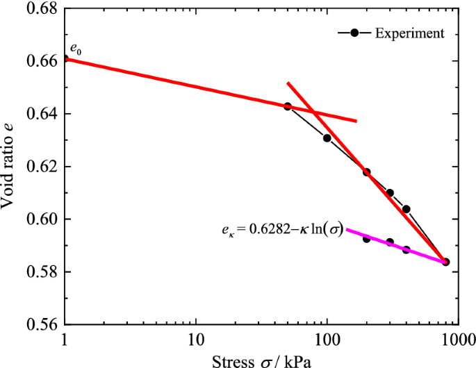
Oedometer test results at 24 h
-
(ii)
M and G are measured by conventional triaxial tests under different confining pressures, where M can also be calculated by effective stress ratio or effective internal friction angle (\(M = {{6\sin \varphi^{\prime}} \mathord{\left/ {\vphantom {{6\sin \varphi^{\prime}} {\left( {3 - \sin \varphi^{\prime}} \right)}}} \right. \kern-0pt} {\left( {3 - \sin \varphi^{\prime}} \right)}}\)). And G can also be calculated according to \(G = {q \mathord{\left/ {\vphantom {q {3\varepsilon_{0}^{vp} }}} \right. \kern-0pt} {3\varepsilon_{0}^{vp} }}\).
-
(iii)
\(\alpha\) and \(\beta\) are parameters describing the viscoplastic flow. They are determined by the nature of the material itself, independent of the stress state. According to the results of Fodil et al. [7], its value can be determined by secondary compression in creep test, stress relaxation test and consolidation test. Yin et al. [36] used the power function form to describe the viscoplastic strain rate and deduced the calculation formulas of \(\alpha\) and \(\beta\) on the basis of the consolidation test of constant strain rate and traditional consolidation test. However, in view of the complexity of scalar multiplier and fractional strain rate in this paper, the parameters \(\alpha\) and \(\beta\) are obtained by fitting analysis with the results of the triaxial creep test. The consistency between the calculated value and the actual value is ensured to be the best.
-
(iv)
The overstress ratio \({{\sigma_{md} } \mathord{\left/ {\vphantom {{\sigma_{md} } {\sigma_{ms} }}} \right. \kern-0pt} {\sigma_{ms} }}\) or \({{f_{d} } \mathord{\left/ {\vphantom {{f_{d} } {f_{s} }}} \right. \kern-0pt} {f_{s} }}\) determines the viscoplastic strain rate. Hinchberger and Rowe [9] proposed a new method to determine the overstress ratio \({{\sigma_{md} } \mathord{\left/ {\vphantom {{\sigma_{md} } {\sigma_{ms} }}} \right. \kern-0pt} {\sigma_{ms} }}\), utilizes parallel yield surface tangents to predict apparent yield surface expansion due to strain rate effects in stress space through elliptical cap formulation, where \(\sigma_{ms}\) and \(\sigma_{md}\) are the current pressures corresponding to static and dynamic yield surface (\(f_{s}\) and \(f_{d}\)), respectively. \(\sigma_{md}\) represents the current stress state of the soil. \(\sigma_{ms}\) reflects the initial state of the soil, which is related to the current stress state, and together with \(\sigma_{md}\) determines the initial creep strain of the soil. Adachi et al. [1] fitted the calculation formula of the parameter \(\sigma_{ms}\) based on the plastic hardening law and the consolidation test. However, the fractional model will limit the calculation formula of Adachi, which is also complex and requires additional fitting parameters. Therefore, parameter \(\sigma_{ms}\) is obtained by triaxial creep strain fitting.
-
(v)
The value range of fractional order r is \(0 < r < 1\). When \(r = 1\) is taken into account, the fractional strain rate of Eq. (19) can be simplified to an integer EVP model, but the fractional creep equation of Eq. (23) can only be degenerated into a linear creep equation. Figure 4 shows the influence of order on strain under the same conditions. It is found that with the increase of r from 0.1 to 1, the creep strain and strain rate of soil show a phenomenon of rapid increase, and when r is 1, the strain and time are linear. It is worth noting that the creep strain at 0–1 h in Fig. 4 is close to zero. Zhou et al. [37, 38] also showed a similar situation when discussing creep strain based on the fractional element model. However, this phenomenon does not occur in all cases, and it seems to be more obvious only when the time step is large. The initial stress of the fractional stress relaxation model established by Yin et al. [34] is unbounded. Both the fractional creep model and the fractional stress relaxation model have partial errors at the initial moment. But the reason for both is the opposite. In the fractional creep model, the time step cannot be performed in an infinite time interval, and the fractional stress relaxation model is just the opposite of the former.
Fig. 4 
Value range of order r
-
(vi)
a and b are the terminals of the stress interval of the fractional derivatives. To some extent, they can qualitatively reflect the growth process of stress. In a specific stress space, all stress components \(\sigma_{ij}\) satisfy \(a < \sigma_{ij} < b\). Sumelka [24] expressed this phenomenon as the virtual field of the stress state and defined the stress interval terminals a and b:
$$a_{ij} = \sigma_{ij}^{a} - \Delta L_{ij} \;{\text{and}}\;b_{ij} = \sigma_{ij}^{b} + \Delta R_{ij}$$(27)where \(\Delta L_{ij}\) and \(\Delta R_{ij}\) are the lengths of the left and right axes in the six-dimensional stress space, respectively, and both are positive, \(\sigma_{ij}^{a} = \sigma_{ij}^{\hbox{min} }\), \(\sigma_{ij}^{b} = \sigma_{ij}^{\hbox{max} }\). When the virtual field is discussed in the conventional triaxial test, it can be considered that the transverse stresses are all equal and uniformly distributed. The normal stress is applied by the sample cap, so it can be considered that the stress is uniformly distributed. Therefore, in the virtual field of the conventional triaxial stress state, it can be considered that there are only two main stresses—confining pressure and normal stress. a and b are the terminals of the stress interval introduced when using the RC fractional derivative is used to predict soil creep. In this paper, a and b are defined as the stress state of soil before creep and after creep stabilization, respectively. It can also be understood as the pre-consolidation pressure and the existing consolidation stress of soil. In conventional triaxial creep tests, a and b can be defined as consolidation pressure and axial pressure of constant load creep respectively.


5 Model validation and discussion
Based on the triaxial undrained shear creep test results of Adachi [1] and Hinchberger and Rowe [9], the effectiveness verification of fractional EVP model and the sensitivity analysis of fractional order r were carried out. The required parameter values are shown in Table 1.
5.1 Model verification
Adachi [1] conducted a series of triaxial creep tests on normally consolidated Fukakusa clay. In the undrained shear creep test, the samples were first consolidated for 24 h under the effective stress of 392 kPa. Then, the creep was started under the action of the deviatoric stresses of 118, 157, 196 and 235 kPa, respectively.
Hinchberger and Rowe [9, 21] carried out a series of laboratory tests on silty clay in the shallow foundation of an artificial experimental embankment in the Sackville area. In the K0 consolidation creep test, the samples were normally consolidated for 24 h under the K0 = 0.76. Then, the creep is started under the action of the deviatoric stresses of 35, 44.5 and 50 kPa, respectively. The model parameters in Table 1 are taken from the above literatures.
Figure 5 shows that the prediction results of Fukakusa clay creep by fractional EVP model and two integer EVP models (Adachi, 1982; Yin, 2008), as well as the comparison with the results of triaxial shear creep test. It is found from the figure that the prediction ability of the integer EVP model is relatively low. When the deviatoric stress is 157 and 235 kPa, Adachi’s EVP model can basically predict the creep behavior of Fukakusa clay. However, the integer EVP model and the test results showed significant differences when the deviatoric stress is 118 and 196 kPa. It is worth noting that the fractional EVP model maintains good accuracy in predicting the creep of Fukakusa clay at different stress levels.

Comparison between fractional model and integer EVP model and experimental results on Fukakusa clay
Figure 6 shows the undrained shear creep results of Sackville clay when the action of deviatoric stress of 35, 44.5 and 50 kPa, respectively, and without considering initial elastic deformation. The prediction capabilities of the fractional model are compared with those of Adachi and Hinchberger’s integer EVP model by means of Fig. 6a–c. It is found that the accuracy of the fractional EVP model in Fig. 6a, b is slightly higher than that of the integer EVP model. In Fig. 6c, the fractional EVP model exhibits slightly lower accuracy at the initial creep moment. This is because the fractional model is built to describe nonlinear creep, so it is weak to describe linear creep.

Comparison between fractional model and integer EVP model and experimental results on Sackville clay
According to the analysis results in Figs. 5 and 6, it is shown that the fractional EVP model maintains good predictive ability when describing the creep behavior of different soils. In addition, the solution process of the fractional EVP model is relatively simple and can reflect the change mechanism of the viscoplastic flow direction (non-orthogonal flow). Therefore, the establishment of fractional EVP model has great significance for predicting soil creep behavior.
5.2 Sensitivity analysis
Figure 7 shows the comparison between the shear creep test data under different conditions and the calculated results when the fractional EVP model’s order increment \({\Delta}r=0.01\). Figure 7a, b shows the correlation analysis of creep strain and order increment of Fukakusa clay. Figure 7c, d shows the evolution of the creep strain of the Sackville clay with the order increment. On the whole, the strain and strain rate of soil creep increase rapidly with the increase in the order. This phenomenon is identical to the order feature of the fractional element model proposed by Zhou [37, 38].

Influence of fractional order r on strain
Figure 7a, b shows calculation results of creep at a deviatoric stress of 196 and 235 kPa after normally consolidation. Figure 7c, d shows the calculation results of creep at a deviatoric stress of 35 and 44.5 kPa after consolidation by K0. The magnitudes of the final creep strains at different orders in Figs. 7a–d are discussed, respectively, as shown in Table 2. The results show that the difference in final creep strain between adjacent orders decreases as the stress level increases. That is to say, the stress level limits the influence of the order on the creep properties of the soil.
6 Conclusions
This paper introduces fractional calculus theory into the EVP model based on modified Cam-Clay model and overstress theory. The fractional EVP strain rate model of soil creep is established, and the fractional creep equation of soil creep is solved by Laplace integral transform. The nonlinear analytical solution of EVP model in creep equation and the description of anomalous diffusion characteristics such as path dependence in creep process of soil are realized.
Through the existing triaxial creep test results, the prediction ability of the fractional EVP model and the influence of the order and creep characteristics and the stress level on the order visualization ability are analyzed. The result shows that the fractional EVP model is better than traditional integer EVP model in solving creep equation and predicting ability. A sensitivity study shows the strain and strain rate of soil creep will increase rapidly with the increase in order. In addition, under the same order increments, the stress level limits the effect of the order increment on the creep characteristics.
References
Adachi T, Oka F (1982) Constitutive equations for normally consolidated clay based on elasto-viscoplasticity. Soils Found 22(4):57–70
Adolfsson K, Enelund M, Olsson P (2005) On the fractional order model of viscoelasticity. Mech Time-Depend Mat 9(1):15–34
Agrawal OP (2007) Fractional variational calculus in terms of Riesz fractional derivatives. J Phys A-Math Theor 40(24):6287–6303
Bjerrum Laurits (1967) Engineering geology of norwegian normally-consolidated marine clays as related to settlements of buildings. Géotechnique 17(2):83–118
Cristescu ND (1993) A general constitutive equation for transient and stationary creep of rock salt. Int J Rock Mech Min 30(2):125–140
Enelund M, Mähler L, Runesson K, Josefson LB (1999) Formulation and integration of the standard linear viscoelastic solid with fractional order rate laws. Int J Solids Struct 36(16):2417–2442
Fodil A, Aloulou W, Hicher PY (1997) Viscoplastic behaviour of soft clay. Géotechnique 47(3):581–591
Frederico GSF, Torres DFM (2010) Fractional Noether’s theorem in the Riesz–Caputo sense. Appl Math Comput 217(3):1023–1033
Hinchberger SD, Rowe RK (2005) Evaluation of the predictive ability of two elastic–viscoplastic constitutive models. Can Geotech J 42(6):1675–1694
Hinchberger SD, Qu G (2009) Viscoplastic constitutive approach for rate-sensitive structured clays. Revue Can De Géotech 46(6):609–626
Katona Michael G (1984) Evaluation of viscoplastic cap model. J Geotech Eng 110(8):1106–1125
Kilbas AAA, Srivastava HM, Trujillo JJ (2006) Theory & applications of fractional differential equations. Elsevier
Karim MR, Gnanendran CT (2014) Review of constitutive models for describing the time dependent behaviour of soft clays. Geomech Geoeng 9(1):1–16
Lu DC, Liang JY, Du XL, Ma C, Gao ZW (2019) Fractional elastoplastic constitutive model for soils based on a novel 3D fractional plastic flow rule. Comput Geotech 105:277–290
Lu DC, Zhou X, Du XL, Wang GS (2019) A 3D fractional elastoplastic constitutive model for concrete material. Int J Solids Struct 165(6):160–175
Liang JY, Lu DC, Zhou X, Du XL, Wu W (2019) Non-orthogonal elastoplastic constitutive model with the critical state for clay. Comput Geotech 116(8):103200
Liao MK, Lai YM, Liu EL, Wan XS (2016) A fractional order creep constitutive model of warm frozen silt. Acta Geotech 12(2):1–13
Perzyna P (1963) The constitutive equations for work-hardening and rate sensitive plastic materials. Proc Vib Probl Wars 4(4):281–290
Roscoe KH (1963) Mechanical behaviour of an idealized ‘wet’ clay. Proc Eur Conf Soil Mech Wiesb 1:47–54
Roscoe KH, Burland JB (1968) On the generalized stress–strain behavior of wet clay. Cambridge University Press, New York, pp 535–609
Rowe RK, Hinchberger SD (1998) The significance of rate effects in modelling the Sackville test embankment. Can Geotech J 35(3):500–516
Sumelka W (2014) Fractional viscoplasticity. Mech Res Commun 56:31–36
Sumelka W (2014) Thermoelasticity in the framework of the fractional continuum mechanics. J Therm Stresses 37(6):678–706
Sumelka W, Nowak M (2016) Non-normality and induced plastic anisotropy under fractional plastic flow rule: a numerical study. Int J Numer Anal Meth Geomech 40(5):651–675
Sumelka W, Nowak M (2017) On a general numerical scheme for the fractional plastic flow rule. Mech Mater 1:1–10
Sun YF, Indraratna B, Carter JP, Marchant T (2017) Application of fractional calculus in modelling ballast deformation under cyclic loading. Comput Geotech 82:16–30
Sun YF, Xiao Y (2017) Fractional order plasticity model for granular soils subjected to monotonic triaxial compression. Int J Solids Struct. https://doi.org/10.1016/j.ijsolstr.2017.03.005
Sun YF, Gao YF, Zhu QZ (2018) Fractional order plasticity modelling of state-dependent behaviour of granular soils without using plastic potential. Int J Plasticity 102(3):53–69
Sun Y, Sumelka W, Gao Y (2020) Advantages and limitations of an α-plasticity model for sand. Acta Geotech 15:1423–1437. https://doi.org/10.1007/s11440-019-00877-9
Welch SWJ, Rorrer RAL, Duren RG (1999) Application of time-based fractional calculus methods to viscoelastic creep and stress relaxation of materials. Mech Time-Depend Mater 3(3):279–303
Yang C, Daemen JJK, Yin JH (1999) Experimental investigation of creep behavior of salt rock. Int J Rock Mech Min 36(2):233–242
Yang YG, Lai YM, Chang XX (2010) Experimental and theoretical studies on the creep behavior of warm ice-rich frozen sand. Cold Reg Sci Technol 63(1–2):61–67
Yin JH, Graham J (1994) Equivalent times and one-dimensional elastic viscoplastic modelling of time-dependent stress–strain behaviour of clays. Can Geotech J 31(1):42–52
Yin DS, Wu H, Cheng C, Chen YQ (2013) Fractional order constitutive model of geomaterials under the condition of triaxial test. Int J Numer Anal Met 37(8):961–972
Yin ZY, Zhang DM, Pierre-Yves H, Huang HW (2008) Modelling of time-dependent behaviour of soft soils using simple elasto–viscoplastic model. Chin J Geotech Eng 30(6):880–888
Yin ZY, Chang CS, Karstunen M, Pierre-Yves H (2010) An anisotropic elastic–viscoplastic model for soft clays. Int J Solids Struct 47(5):665–677
Zhou HW, Wang CP, Han BB, Duan QZ (2011) A creep constitutive model for salt rock based on fractional derivatives. Int J Rock Mech Min 48(1):116–121
Zhou HW, Wang CP, Mishnaevsky L, Duan ZQ, Ding JY (2013) A fractional derivative approach to full creep regions in salt rock. Mech Time-Depend Mater 17(3):413–425
Acknowledgments
This research was supported by the National Natural Science Foundation of China (Grant Nos. 11962016, 51978320). The authors are thankful to the reviewers for their insightful and constructive comments.
Author information
Authors and Affiliations
Corresponding author
Additional information
Publisher's Note
Springer Nature remains neutral with regard to jurisdictional claims in published maps and institutional affiliations.
Rights and permissions
About this article

Cite this article
Zhou, F., Wang, L. & Liu, H. A fractional elasto-viscoplastic model for describing creep behavior of soft soil. Acta Geotech. 16, 67–76 (2021). https://doi.org/10.1007/s11440-020-01008-5
Received:
Accepted:
Published:
Issue Date:
DOI: https://doi.org/10.1007/s11440-020-01008-5