Analysis of exact tail asymptotics for singular random walks in the quarter plane

Abstract

In this paper, we consider all singular cases of random walks in the quarter plane. Specifically, exact light tail asymptotics for stationary probabilities are obtained for all singular random walks.

1 Introduction

Tail behaviour of stationary probabilities for random walks in the quarter plane has long been a key issue, because not only its theoretical interest, but also its important applications. For a detailed literature review and recent development of studies, we refer readers to Miyazawa [11, 12] and Li and Zhao [9, 10].

Let X ₊, X ₁, X ₂, and X ₀ be random variables having the distributions, respectively, p _i,j , where i,j=0,±1; $p^{(1)}_{i,j}$, where i=0,±1 and j=0,1; $p^{(2)}_{i,j}$, where i=0,1 and j=0,±1; and $p^{(0)}_{i,j}$, where i,j=0,1. Then the random walk considered in this paper is a two-dimensional discrete-time Markov chain L _t on the state space $S=\mathbb{Z}_{+}^{2}= \{(m,n); m,n = 0, 1, 2, \ldots\}$, partitioned as $\mathbb{Z}_{+}^{2}= S_{+} \cup S_{1} \cup S_{2} \cup S_{0}$, where S ₊={(m,n);m,n=1,2,…}, S ₁={(m,0);m=1,2,…}, S ₂={(0,n);n=1,2,…} and S ₀={(0,0)}, with the following transition probabilities:

Let

When M≠0, a necessary and sufficient condition for stability was obtained in Fayolle, Iasnogorodski, and Malyshev [3] and amended by Kobayashi and Miyazawa (Lemma 2.1 of [7]).

Theorem 1.1

(Theorem 1.2.1 in [3] and Lemma 2.1 in [7])

When M≠0, the random walk is ergodic if and only if one of the following three conditions holds:

• 1. M _x <0, M _y <0, $M_{x}M_{y}^{(1)}-M_{y}M_{x}^{(1)}<0$, and $M_{y}M_{x}^{(2)}-M_{x}M_{y}^{(2)}<0$;

• 2. M _x <0, M _y ≥0, $M_{y}M_{x}^{(2)}-M_{x}M_{y}^{(2)}<0$, and $M_{x}^{(1)}<0$ if $M_{y}^{(1)}=0$;

• 3. M _x ≥0, M _y <0, $M_{x}M_{y}^{(1)}-M_{y}M_{x}^{(1)}<0$, and $M_{y}^{(2)}<0$ if $M_{x}^{(2)}=0$.

Throughout the paper, we assume that the random walk is stable and denote the joint stationary probability vector by π _m,n . For this random walk, the fundamental form (for example, see p. 5 of [3]) is given by

$$ -h(x,y)\pi(x,y)=h_{1}(x,y) \pi_1(x)+h_{2}(x,y)\pi_2(y)+h_{0}(x,y) \pi_{0,0}, $$

(1.1)

where

with

By simple algebra, we obtain

(1.2)

(1.3)

(1.4)

where ′ is the derivative of a function. The above expressions will be used to simplify the stability condition in later sections.

Definition 1.1

A random walk in the quarter plane is called singular if h(x,y), as a polynomial of two complex variables x and y, is either reducible or of degree one in at least one variable.

A necessary and sufficient condition for a random walk to be singular was obtained in [3] and is stated as follows.

Lemma 1.1

(Lemma 2.3.2 in [3])

The random walk is singular if and only if one of the following conditions holds:

• 1. There exists (i,j) such that only p _i,j >0 and p _−i,−j >0;

• 2. There exists i with |i|=1 such that for any j, p _i,j =0;

• 3. There exists j with |j|=1 such that for any i, p _i,j =0.

Based on the above lemma, it is easy to see there are a total of eight possible different cases (or transition diagrams) for the singular random walks, which are depicted in Fig. 1 and Fig. 2.

Fig. 1

Singular cases corresponding to part 1 of Lemma 1.1

Fig. 2

Singular cases corresponding to part 2 and part 3 of Lemma 1.1

In the analysis throughout the paper, we assume a positive probability for every possible transition in all singular cases. Only minor modifications might be needed if the probability were to be zero for a possible transition.

Remark 1.1

Our focus is on a stable random walk with light-tailed behaviour of its stationary probabilities, which is equivalent to the case of M≠0. By light-tailed behaviour, we mean that both complex functions π ₁(x) and π ₂(y) have a convergence radius greater than 1, which is equivalent to both π _i,0 and π _0,j being light-tailed. When M=0, Lemma 3.3 in [7] showed that the random walk is heavy-tailed. When M≠0, all random walks are light-tailed. For non-singular cases, this was proved in [3] (for example, Corollary 3.2.4). For the singular cases, this is also true. In fact, analytic continuation in each singular case is automatically clear from the detailed analysis provided in the following sections except for case 3. In this case, analytic continuation is not immediately clear and the kernel method in [3] seems not feasible. Instead, one can use other methods (for example, He, Li, and Zhao [6], [3, 11], or Guillemin and Simonian [5]) to show that both π _i,0 and π _0,j are light-tailed.

The literature study has mainly been focusing on non-singular random walks. Tail asymptotic analysis for singular cases is only available for a few specific models, for example, the priority queues (see Abate and Whitt [1] and Li and Zhao [8] for details and relevant references). It is of interest to provide a complete description of the tail asymptotic properties for all singular cases, which is the purpose of this paper. Based on the fundamental form (1.1), a modified kernel method is applied to confirm that the exact tail asymptotics for boundary probabilities π _m,0 (and π _0,n ) for the singular cases have the same four types as that for the non-singular cases. This is also true for the two marginal distributions: $\pi^{(1)}_{m} = \sum_{n} \pi_{m,n}$ and $\pi^{(2)}_{n} = \sum_{m} \pi_{m,n}$, but details will not be presented in the paper since they only require some minor efforts. However, a new type of exact tail asymptotic property for joint probabilities π _m,n along a coordinate direction, say for a fixed n as m→∞, can appear for a reducible h(x,y). For tail asymptotic properties in the joint distribution along a coordinate direction, we define and analyze the generating functions:

Notice that φ ₀(x)=π ₁(x) and ψ ₀(y)=π ₂(y). Recursive relationships will be obtained for φ _j (x) and ψ _i (y), respectively, based on the balance equations of the random walk:

(1.5)

(1.6)

(1.7)

(1.8)

(1.9)

(1.10)

Throughout the paper, a Tauberian-like theorem (see, for example, Theorem 4 in Bender [2] or Corollary 2 in Flajolet and Odlyzko [4]) is frequently used for asymptotic analysis.

The rest of the paper is organized as follows: In Sect. 2 to Sect. 6, all eight singular cases are analyzed and exact tail asymptotics are obtained for boundary probabilities (π _m,0 and π _0,n ) as well as for joint probabilities along a coordinate direction (π _m,j for j≥1 and π _i,n for i≥1). Finally, concluding remarks are offered in Sect. 7.

2 Exact tail asymptotics for case 1 and case 2

Since these two cases are symmetric, we provide a detailed analysis only for case 1. Corresponding results for case 2 can be easily obtained by symmetry.

In this case, we have

(2.1)

(2.2)

Hence,

$$ h(x,y)= \bigl[p_{-1,0}-(1-p_{0,0})x+p_{1,0}x^2 \bigr]y. $$

(2.3)

To make h=0, we should have y=0 or

$$x = \frac{(1-p_{0,0}) \pm\sqrt{(1-p_{0,0})^2 - 4p_{1,0}p_{-1,0}}}{2p_{1,0}} = \frac{(p_{-1,0}+p_{1,0})\pm |p_{-1,0}-p_{1,0}|}{2p_{1,0}}. $$

Under the stability condition, we have M _x <0 since M _y =0 (remember that we are considering the light-tailed case only for M≠0). The condition M _x <0 is equivalent to p _−1,0>p _1,0. Therefore,

$$x = \begin{cases} p_{-1,0}/p_{1,0}, \\ 1. \end{cases} $$

Let x=1 and |y|≤1. Then π(1,y) is finite and the fundamental form leads to

$$h_1(1,y) \pi_1(1) + h_2(1,y) \pi_2(y) + h_0(1,y) \pi_{0,0} =0, $$

or

$$ \pi_2(y) = - \frac{h_1(1,y) \pi_1(1) + h_0(1,y) \pi _{0,0}}{h_2(1,y )} $$

(2.4)

if h ₂(1,y)≠0. Notice that h ₂(1,y)=(a ₂(1)y−c ₂(1))(y−1) gives two zeros: y=1 and y=c ₂(1)/a ₂(1)>1 according to the stability condition. Also, y=1 is a zero of the numerator in (2.4) since π ₂(y) is the generating function of a probability sequence that should be finite at y=1. Specifically, since

$$h_1(1,y) = a_1(1) (y-1),\qquad h_0(1,y)= a_0(1) (y-1), $$

we have

$$ \pi_2(y) = \frac{a_1(1) \pi_1(1) + a_0(1) \pi _{0,0}}{c_2(1)-a_2(1)y}. $$

(2.5)

Obviously, y=c ₂(1)/a ₂(1) is the dominant simple pole of π ₂(y), which leads to an analytic continuation of π ₂(y) and (2.5) implies that

$$ \pi_{0,j+1} = c \biggl(\frac{a_2(1)}{c_2(1)} \biggr)^j, \quad j \geq0. $$

(2.6)

Therefore, for large j,

$$\pi_{0,j+1} \sim c \biggl( \frac{a_2(1)}{c_2(1)} \biggr)^j, $$

where

$$ c= \frac{a_1(1) \pi_1(1) + a_0(1) \pi_{0,0}}{c_2(1)}. $$

(2.7)

It follows from (2.6) that c=π _0,1 and according to the definition of π ₂(y), c=π ₂(0).

Now, using expression (2.5) in the fundamental form and let y=0 leads to

$$\pi_1(x) = -\frac{c_2(x) c + b_0(x) \pi_{0,0}}{b_1(x)}. $$

b ₁(x) has two zeros:

$$ x_{b_{1}}^{\pm} = \frac{1-p_{0,0}^{(1)}\pm \sqrt{(1-p_{0,0}^{(1)})^{2}-4p_{-1,0}^{(1)}p_{1,0}^{(1)}}}{2p_{1,0}^{(1)}}, $$

(2.8)

of which, $x_{b_{1}}^{-} \leq1$ is removable and $x_{b_{1}}^{+} >1$ is the dominant pole of π ₁(x). This gives an analytic continuation of π ₁(x) and implies that for large i,

$$\pi_{i+1,0} \sim c_{1,0} \biggl( \frac{1}{x_{b_1}^+} \biggr)^i, $$

where c _1,0 is a constant that can be expressed in terms of c and π _0,0, which will be explicitly determined in Sect. 2.3. We therefore postpone the expression of c _1,0 to Sect. 2.3.

For tail asymptotics along a coordinate direction, we consider the sequence of generating functions φ _n (x) or ψ _n (y).

2.1 Along the x-direction

By multiplying balance equations (1.6), (1.7), and (1.10) to an appropriate power of y and taking summations, and after some simplifications, we have

where

Therefore,

Note that the two zeros of b(x) are given by

$$ x_{b}^{\pm} = \frac{1-p_{0,0}\pm\sqrt {(1-p_{0,0})^{2}-4p_{-1,0}p_{1,0}}}{2p_{1,0}}, $$

(2.9)

of which $x_{b}^{-} \leq1$ is removable and $x_{b}^{+}$ is a simple pole of φ _j (x), j≥2. For random walks in case 1, we specifically have $x_{b}^{-}=1$ and $x_{b}^{+}=p_{-1,0}/p_{1,0}$. Using the Tauberian-like theorem to the above functions φ _j (x), j≥0, we immediately have the following tail asymptotic properties.

Theorem 2.1

For the case 1 singular random walk, we have the following tail asymptotic properties along the x-direction: for large i,

where all constants c _1,0, $c^{(t)}_{1,1}$ for t=a,b,c and c _1,j for j≥2 are independent of i and explicitly determined in Sect. 2.3.

Remark 2.1

The Tauberian-like theorem provides a relationship between the asymptotic property at the dominant singularity of the generating function and the tail asymptotic property of the coefficients (probabilities of interest) of the function. Therefore, the decay rate is the reciprocal of the dominant singularity of the function. For example, the dominant singularity of φ ₁(x) is given by the smallest zero of the functions b(x) and b ₁(x) since at which the numerator of the expression for φ ₁(x) is not zero.

2.2 Along the y-direction

By using balance equations (1.8), (1.9), and (1.10) and a similar argument to that in Sect. 2.1, we have

where

Let $y^{\ast}=\frac{c_{2}(1)}{a_{2}(1)}$. By induction on n, we obtain

$$\lim_{y\rightarrow y^{\ast}} \biggl( 1-\frac {c_{2}(1)}{a_{2}(1)} \biggr) \psi_{n}(y)=c_{2,n}, \quad n \geq0, $$

and

where c _2,0=c. Solving the above second-order relations, we obtain

$$c_{2,n}=A \biggl( \frac{p_{1,0}}{p_{-1,0}} \biggr)^{n-1}+B, \quad n \geq1. $$

For determining A and B, from $h_{2}(1,y^{*})=\tilde{b}_{2}(y^{\ast})+\tilde{a}_{2}(y^{\ast})=0$ and

we obtain

$$p_{-1,0} \biggl[ A\frac{p_{1,0}}{p_{-1,0}}+B \biggr]+\bigl [p_{-1,0}-(1-p_{0,0}) \bigr](A+B)=0, $$

which yields B=0. From $\tilde{c}(y^{\ast})(A+B)+\tilde{b}_{2}(y^{\ast})c=0$, we get

$$A=-\frac{\tilde{b}_{2}(y^{\ast})c}{\tilde{c}(y^{\ast})}, $$

where c is given in (2.7).

Finally, the asymptotic properties follow from the Tauberian-like theorem.

Theorem 2.2

For the case 1 singular random walk, we have the following tail asymptotic properties along the y-direction: for large j

Remark 2.2

Case 2 is completely symmetric to case 1, for which one can easily find the result.

2.3 Determinations of coefficients in 2.1

Coefficients c _1,0, $c^{(t)}_{1,1}$ for t=a,b,c, and c _1,j for j≥2 in Theorem 2.1 can be expressed, according to the analysis in Sect. 2.1 and the Tauberian-like theorem, as

and for j≥2,

In the above expressions, all components are explicitly expressed in terms of system parameters and probabilities π _0,0, π _0,1 (noting that c=π _0,1) and π _0,2. In the following, we express π _0,1 and π _0,2, and π ₁(1) and π ₂(1) (therefore, π(1,1)) in terms of π _0,0. This also leads to a determination of π _0,0 according to the normalization condition: 1=π(1,1)+π ₁(1)+π ₂(1)+π _0,0.

First, from

$$\pi_{1}(x)=\frac{a_{0}^{\ast}(x)}{b_{1}(x)}=\frac{a_{0}^{\ast }(x)}{p_{1,0}^{(1)}(x-x_{b_{1}}^{-})(x-x_{b_{1}}^{+})} $$

we conclude that since $0<x_{b_{1}}^{-}<1$, $x_{b_{1}}^{-}$ is also a zero of the numerator, i.e.

$$a_{0}^{\ast}\bigl(x_{b_{1}}^{-} \bigr)=-c_{2}\bigl(x_{b_{1}}^{-}\bigr) \pi_{0,1} - b_{0}\bigl(x_{b_{1}}^{-}\bigr) \pi_{0,0}=0. $$

Therefore, we can express π _0,1 in terms of π _0,0 as follows:

$$ \pi_{0,1} = -\frac{b_{0}(x_{b_{1}}^{-})\pi _{0,0}}{c_{2}(x_{b_{1}}^{-})}. $$

(2.10)

Using (2.10) we express π ₁(1) in terms of π _0,0:

$$ \pi_{1}(1) = \frac{c_{2}(1)\pi_{0,1}+b_{0}(1)\pi_{0,0}}{b_{1}(1)} =-t_{1}\pi_{0,0}, $$

(2.11)

where

$$t_{1}=-\frac{c_{2}(1)\frac {-b_{0}(x_{b_{1}}^{-})}{c_{2}(x_{b_{1}}^{-})}+b_{0}(1)}{b_{1}(1)}. $$

Now, we can use the above result to express π ₂(1) in terms of π _0,0 as follows. From

$$\pi_{2}(y)=\frac{a_{1}(1)\pi_{1}(1)+a_{0}(1)\pi_{0,0}}{c_{2}(1)-a_{2}(1)y} $$

we obtain

$$\pi_{2}(1) = -\frac{a_{1}(1)t_{1}+a_{0}(1)}{c_{2}(1)-a_{2}(1)}\pi _{0,0}=-t_{2} \pi_{0,0}, $$

where

$$t_{2}=-\frac{a_{1}(1)t_{1}+a_{0}(1)}{c_{2}(1)-a_{2}(1)}. $$

For expressing π(1,1) in terms of π _0,0, we consider the following expression, which is valid for all cases:

from which, by using the above result, we have

$$\pi(1,1)=t_{3}\pi_{0,0}, $$

where

$$t_{3}= \frac{ \{ x[p_{1,1}^{(1)}+p_{1,0}^{(1)}]-[p_{-1,0}^{(1)}+p_{-1,1}^{(1)}] \} t_{1}+ \tilde{a}_{2}(1)t_{2}+ [ p_{1,0}^{(0)}+p_{1,1}^{(0)} ] }{(p_{1,1}+p_{1,0})x-(p_{-1,1}+p_{-1,0})}. $$

Remark 2.3

In case 1, p _1,1=p _−1,1=0. However, we keep p _1,1 and p _−1,1 in the expression for t ₃ since in this way the expression becomes valid for case 5 as well.

Finally, π _0,0 is determined as

$$\pi_{0,0}=\frac{1}{1+t_{1}+t_{2}+t_{3}} $$

and

$$\pi_{0,2}=\pi_{0,1}\frac{a_{2}(1)}{c_{2}(1)} $$

from the Taylor expansion of (2.4).

3 Exact tail asymptotics for case 3

In this case, we have

$$a(x)=p_{1,1} x^2, \qquad b(x)=-(1-p_{0,0})x, \qquad c(x)=p_{-1,-1}; $$

$$\tilde{a}(y) = p_{1,1}y^{2}, \qquad\tilde{b}(y) = -(1-p_{0,0})y, \qquad\tilde{c}(y) = p_{-1,-1}. $$

Therefore, the kernel function h is given as

(3.1)

Since M _x =M _y in this case, for the system to be stable we need M _x =M _y <0 or p _1,1<p _−1,−1.

From balance equations, we also have

and

where $\tilde{a}_{i}^{\ast}(y)$, i≥0, and $a_{j}^{\ast}(x)$, j≥0, are given in Sects. 2.1 and 2.2, respectively. In fact, the above recursive relations hold for all singular cases.

Remark 3.1

In this case, one can see easily that the system is stable if and only if (i) p _1,1<p _−1,−1; (ii) $p_{1,0}^{(1)}-p_{0,1}^{(1)}-p_{-1,0}^{(1)}- 2p_{-1,1}^{(1)}<0$; and (iii) $p_{0,1}^{(2)}-p_{1,0}^{(2)}-p_{0,-1}^{(2)}-2p_{1,-1}^{(2)}<0$.

3.1 Asymptotics along a coordinate direction

Consider the function π ₁(x) first, which will lead to the exact tail asymptotic property for π _i,0.

This singular case is the only case for which the provided analysis in this paper could not automatically lead to analytic continuation to the circle beyond the unit one. Instead, according to Remark 1.1, we assume that the radius of convergence for both π ₁(x) and π ₂(y) is greater than 1. Under this assumption, we can choose proper $y=\frac{1}{x}$ as a function of x to be Y(x)=1/x to make the right-hand side of the fundamental form equal to zero, or

$$\pi_{1}(x)=\frac{-h_{2}(x,Y(x))\pi_{2}(Y(x))-h_{0}(x,Y(x))\pi _{0,0}}{h_{1}(x,Y(x))} $$

at least in the region: ε≤|x|<R, where 0<ε<1 and R is the dominant singular point of π ₁(x). Since π ₂(Y(x)) is analytic for |x|>1, it is easy to see that the zeros of h ₁(x,Y(x)) are the only potential poles of π ₁(x).

To determine the dominant pole of π ₁(x), we notice that h ₁(1,Y(1))=0 and $h_{1}^{\prime}(1,Y(1))<0$ from ergodic condition. Therefore, it is easy to see that h ₁(x,Y(x)) has two zeros in [−1,1] and one zero in (1,∞). Let x _dom be the zero of h ₁(x,Y(x)) in (1,∞), which is the dominant simple pole. It is clear now that π _i,0 has an exact geometric tail with the decay rate $\frac{1}{x_{\mathrm {dom}}}$. Here, x _dom can be easily found by noticing

which leads to

$$ x_{\mathrm{dom}}= \frac {p_{-1,0}^{(1)}+p_{-1,1}^{(1)}+p_{0,1}^{(1)}+\sqrt{ [p_{-1,0}^{(1)}+p_{-1,1}^{(1)}+p_{0,1}^{(1)} ]^{2}+4p_{1,0}^{(1)}p_{-1,1}^{(1)}}}{2p_{1,0}^{(1)}}. $$

(3.2)

We can similarly determine that π _0,j has a geometric solution by letting $x=X(y)=\frac{1}{y}$. To determine the dominant simple pole y _dom for π ₂(y), which is the zero of h ₂(X(y),y) in (1,∞). Now, we show that $x_{\mathrm{dom}}y_{\mathrm{dom}}=\frac{p_{-1,-1}}{p_{1,1}}$. In fact, since

and

we obtain

$$Y(x_{\mathrm{dom}})X(y_{\mathrm{dom}}) =\frac{p_{-1,-1}}{p_{1,1}}. $$

Therefore,

$$x_{\mathrm{dom}}y_{\mathrm{dom}} =\frac{p_{-1,-1}}{p_{1,1}}. $$

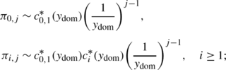
By induction, we can show easily that ψ _i (y), i≥1 (φ _j (x), j≥1) has the same dominant singular point as ψ ₀(y) (φ ₀(x)). Using the recursive relations for ψ _i (y) (φ _j (x)) and then solving the corresponding second-order relation as we did in Sect. 2.2, we obtain the following theorem.

Theorem 3.1

For the singular random walk in case 3, we have the following exact tail asymptotic properties:

• 1. (Along the x-direction): For large i,

  

  (3.3)
  

  (3.4)

  where c ₁ and D ₁ are constants independent of i and j.

• 2. (Along the y-direction): For large j,

  

  (3.5)
  

  (3.6)

  where c ₂ and D ₃ are constants independent of i and j.

Remark 3.2

The coefficients c ₁, c ₂, D ₁, and D ₂ are independent of i and j. We did not provide expressions for these coefficients though it is possible. The main reason is that expressions for them involve information about generating functions π ₁(x) or π ₂(y) for which we do not have explicit expressions. Therefore, these coefficients cannot be explicitly expressed in terms of system parameters in general.

4 Exact tail asymptotic for singular case 4

First, notice that this is not a symmetric case to case 3. In this case, we have

(4.1)

(4.2)

and

(4.3)

To make h(x,y)=0, we need either y=x or

$$y= \frac{p_{1,-1}}{p_{-1,1}} x. $$

Since in this case M _x =−M _y , there are two possibilities for the system to be stable:

(4.4)

(4.5)

Analysis for these two possibilities are completely symmetric. Therefore, we only provide details for M _y >0, i.e. p _−1,1>p _1,−1.

4.1 Along the y-direction

When y=x and |x|≤1, π(x,y)<∞. It follows from the fundamental form that

$$ \pi_{1}(x)=-\frac{h_{2}(x,x)\pi _{2}(x)+h_{0}(x,x)\pi_{0,0}}{h_{1}(x,x)}. $$

(4.6)

On the other hand, when $y=\frac{p_{1,-1}}{p_{-1,1}}x$ and |x|≤1, we clearly have |y|<1. It follows from the fundamental form again that

$$ \pi_{1}(x)=-\frac{h_{2} ( x,\frac {p_{1,-1}}{p_{-1,1}}x ) \pi_{2} ( \frac{p_{1,-1}}{p_{-1,1}}x ) +h_{0} ( x,\frac{p_{1,-1}}{p_{-1,1}}x ) \pi_{0,0}}{h_{1} ( x,\frac{p_{1,-1}}{p_{-1,1}}x ) }. $$

(4.7)

Combining Eqs. (4.6) and (4.7), and substituting x by y in all expressions lead to, when |y|≤1,

$$ \pi_{2}(y)=\frac{N(y)}{h_{1} (y,\frac {p_{1,-1}}{p_{-1,1}}y ) h_{2}(y,y)}, $$

(4.8)

where

Let y _dom be the dominant singular point of π ₂(y). Since $|\frac{p_{1,-1}}{p_{-1,1}}y| <|y_{\mathrm{dom}}|$ when |y|<|y _dom|, $\pi_{2} ( \frac{p_{1,-1}}{p_{-1,1}}y )$ is analytic on the disk |y|≤|y _dom|+ε for some ε>0. It follows that y _dom is either a zero of $h_{1} ( y,\frac{p_{1,-1}}{p_{-1,1}}y )$ or a zero of h ₂(y,y).

For the case of $\max \{p_{0,1}^{(1)},p_{1,1}^{(1)},p_{1,0}^{(1)}\}>0$, since h ₁(0,0)≥0, $h_{1} ( 1,\frac{p_{1,-1}}{p_{-1,1}} ) <0$, $h_{1} ( -1,-\frac{p_{1,-1}}{p_{-1,1}} ) >0$ and $h_{1} ( y,\frac{p_{1,-1}}{p_{-1,1}}y ) >0$ when y is sufficiently large, $h_{1} ( y,\frac{p_{1,-1}}{p_{-1,1}}y )$ has two positive zeros, $y_{1}^{\prime}$ and y ₁, with $y_{1}^{\prime}\in[0,1]$ and y ₁∈(1,∞), as well as a negative zero, $y_{1}^{\prime\prime} \in(-1,-\infty)$, if $p_{1,1}^{(1)}>0$. By simple algebra, we can show easily $|y_{1}^{\prime\prime}|\geq y_{1}$ and $|y_{1}^{\prime \prime}|=y_{1}$ if and only if $\max \{p_{0,1}^{(1)},p_{0,-1}^{(1)},p_{1,0}^{(1)}\}=0$.

In the case of $\max\{p_{0,1}^{(1)},p_{1,1}^{(1)},p_{1,0}^{(1)}\}=0$, $h_{1} ( y,\frac{p_{1,-1}}{p_{-1,1}}y )$ has only one zero $y_{1}^{\prime}$. In this case, we let |y ₁|=∞. Similarly, if $p_{1,1}^{(2)}>0$, h ₂(y,y) has three zeros: 1, y ₂ and $y_{2}^{\prime\prime}$, where

Since h ₂(1,1)=0 and $h_{2}^{\prime}(1,1)<0$, y ₂∈(1,∞). Clearly, $|y_{2}^{\prime\prime}|>y_{2}$. Note that $h_{2}^{\prime}(1,1)<0$ follows from $h_{2}^{\prime}(1,1)=M_{x}^{(2)}+M_{y}^{(2)}$ and the stability condition. In the case of $p_{1,1}^{(2)}=0$, $y_{2}= \frac{p_{0,-1}^{(2)}}{1-p_{0,-1}^{(2)}-p_{1,-1}^{(2)}}$ and $y_{2}^{\prime\prime}$ does not exist, so we let $y_{2}^{\prime \prime}=\infty$. Hence, |y _dom|=min{y ₁,y ₂}. Assume N(y)≠0 (see Remark 4.1 for the case of N(y)=0). Applying the Tauberain-like theorem on ψ ₀(y), we obtain the asymptotics for π _0,j . Using a similar argument to that for Theorem 3.1, we obtain the asymptotics for π _i,j for a fixed i≥1.

Applying the Tauberain-like theorem on ψ ₀(y), we obtain the asymptotics for π _0,j and using a similar argument used for Theorem 3.1, we obtain the asymptotics for π _i,j for each fixed i≥1 as given below.

Theorem 4.1

For the singular random walk in case 4, we have the following exact tail asymptotic properties:

• 1.

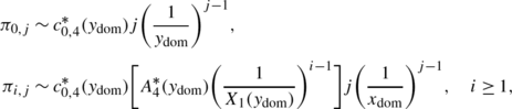
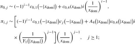
  • (a) If y ₁<y ₂ and $\max\{p_{0,1}^{(1)},p_{1,0}^{(1)},p_{-1,0}^{(1)}\}\neq0$, or if y ₂<y ₁, we have, for large j,

    

  • (b) If y ₁<y ₂ and $\max \{p_{0,1}^{(1)},p_{1,0}^{(1)},p_{-1,0}^{(1)}\}=0$, we have, for large j,

    

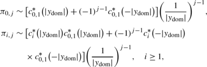
  where $X_{1}(y)=\frac{p_{1,-1}}{p_{-1,1}}y$, X ₀(y)=y, and

  
• 2.

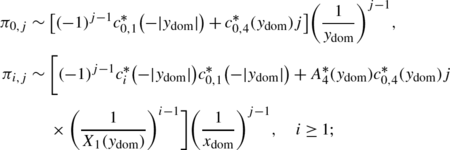
  • (a) If y ₁=y ₂ and $\max \{p_{0,1}^{(1)},p_{1,0}^{(1)},p_{-1,0}^{(1)}\}=0$, we have, for large j,

    

  • (b) If y ₁=y ₂ and $\max \{p_{0,1}^{(1)},p_{1,0}^{(1)},p_{-1,0}^{(1)}\}\neq0$, we have, for large j,

    

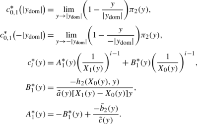
    where

    $$ c_{0,4}^{\ast}(y_{\mathrm{dom}})=\lim_{y\rightarrow y_{\mathrm {dom}}} \biggl( 1-\frac{y}{y_{\mathrm{dom}}} \biggr)^{2}\pi_{2}(y) \quad\text{\textit{and} } \quad A_{4}^{\ast}(y)=\frac{-\tilde{b}_{2}(y)}{\tilde{c}(y)}. $$

Remark 4.1

In the case of N(y _dom)=0, y _dom will be a simple pole and, therefore, π _i,j has an exact geometric decay. Since N(y) is a function of $\pi_{2} ( \frac{p_{1,-1}}{p_{-1,1}}y )$ when |y|≤y _dom, where π ₂(y) is not explicitly determined, we are unable to give a simple characterization for N(y _dom)=0. For some special cases, it becomes possible. For example, if y ₁=y ₂, we can show that it is equivalent to $h_{1} ( y_{2},\frac{p_{1,-1}}{p_{-1,1}}y_{2} ) =0$, or a simple characterization of N(y)=0 is given by

$$a_{1}(y_{2})\frac{p_{1,-1}}{p_{-1,1}}y_{2}+b_{1}(y_{2})=0. $$

4.2 Along the x-direction

Let x _dom be the dominant singular point of π ₁(x). From (4.6), x _dom is either a zero of h ₁(x,x) or the dominant singular point of π ₂(x).

It is easy to see that h ₁(x,x) has three zeros: 1, x ₁>0 and x ₂<0 with |x ₂|>x ₁ if $p_{1,1}^{(1)}\neq0$. Let $y_{1}^{\ast}=x_{1}$ if x ₁>1 (noting that x ₁>1 if and only if $p_{-1,0}^{(1)}>p_{0,1}^{(1)}+2p_{1,1}^{(1)}+p_{1,0}^{(1)}$), otherwise let $y_{1}^{\ast}=\infty$. Since $\frac{p_{1,-1}}{p_{-1,1}}x<x$ when x>0, $h_{1} (x,\frac{p_{1,-1}}{p_{-1,1}}x ) <h_{1} ( x,x )$. Also, $y_{1}^{\ast}<y_{1}$ if x ₁>1. Thus, $|x_{\mathrm{dom}}|=\min\{y_{1}^{\ast},y_{1},y_{2}\}$. Applying the Tauberian-like theorem on φ ₀(x), we obtain the tail asymptotics for π _i,0. Using a similar argument used for Theorem 3.1 to π _i,j for fixed j≥1, we obtain the following tail asymptotic properties.

Theorem 4.2

For the singular random walk in case 4, we have the following exact tail asymptotic properties: for large i,

• 1.

  • (a) If $y_{1}<\min\{y_{2},y_{1}^{\ast}\}$ and $\max \{p_{0,1}^{(1)},p_{1,0}^{(1)},p_{-1,0}^{(1)}\}\neq0$; or (b) if $y_{2}< \min\{y_{1},y_{1}^{\ast}\}$; or (c) if $y_{1}^{\ast}<y_{2}$, then

    

  • (d) If $y_{1}<\min\{y_{1}^{\ast},y_{2}\}$ and $\max \{p_{0,1}^{(1)},p_{1,0}^{(1)},p_{-1,0}^{(1)}\}=0$, then

    

  where $Y_{1}(x)=\frac{p_{1,-1}}{p_{-1,1}}x$, Y ₀(x)=x,

  
• 2.

  • (a) If $y_{1}=y_{2}<y_{1}^{\ast}$ and $\max \{p_{0,1}^{(1)},p_{1,0}^{(1)},p_{-1,0}^{(1)}\}=0$, then

    

  • (b) If $y_{1}^{\ast}=y_{2}$; or (c) if $y_{1}=y_{2}<y_{1}^{\ast}$ and $\max \{p_{0,1}^{(1)},p_{1,0}^{(1)},p_{-1,0}^{(1)}\}\neq0$, then

    

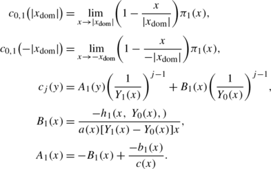
  where

  $$A_{4}(x)=\frac{-b_{1}(x)}{c(x)},\quad\text{\textit{and}}\quad c_{0,4}(x_{\mathrm {dom}})= \lim_{x \rightarrow x_{\mathrm{dom}}} \biggl( 1-\frac{x}{x_{\mathrm {dom}}} \biggr)^{2} \pi_{1}(x). $$

Remark 4.2

For M _x >0, the tail asymptotic properties can be obtained in the same fashion simply by switching x and y.

5 Exact tail asymptotics for case 5 and case 6

These two cases are symmetric. We only provide details for case 5. Corresponding results can be easily obtained by symmetry.

In case 5, we have

5.1 Along the x-direction

Using the same method as in Sect. 2.1, we have

(5.1)

The above recursive relations give a general solution

(5.2)

(5.3)

where A ₀(x) is determined from expressions (5.2) and (5.3) for j=1, together with (5.1) as follows:

$$A_{0}(x)=\frac{-a_{1}(x)\varphi_{0}(x)}{b(x)}=\frac{-a_{1}(x) \frac{a_{0}^{\ast}(x)}{b_{1}(x)}}{b(x)}=\frac{-a_{1}(x)a_{0}^{\ast }(x)}{b(x)b_{1}(x)}. $$

From the expression for φ _j (x), it is clear that the zeros of b(x) and b ₁(x) are only possible poles of φ _j (x), j≥0, and it does not have any other singular points.

Based on the expressions for b(x) and b ₁(x), the zeros $x_{b}^{\pm }$ and $x_{b_{1}}^{\pm}$ of them are given, respectively, by (2.9) and (2.8). Moreover, since b(1)<0 and b(0)>0, we have $0<x_{b}^{-}<1<x_{b}^{+}$. Similarly, $0<x_{b_{1}}^{-}<1<x_{b_{1}}^{+}$. This means that only $x_{b}^{+}$ and $x_{b_{1}}^{+}$ are possible poles of φ _j (x).

When j=0, the following lemma follows immediately from the expression for φ ₀(x) in (5.2).

Lemma 5.1

For j=0, we have for large i,

$$\pi_{i+1,0} \sim c_{1,0} \biggl( \frac{1}{x_{b_1}^{+}} \biggr)^{i}, $$

where

$$c_{1,0}=\frac{-a_{0}^{\ast }(x_{b_{1}}^{+})}{p_{1,0}^{(1)}x_{b_{1}}^{+} ( x_{b_{1}}^{+}-x_{b_{1}}^{-} ) }. $$

For asymptotic properties of φ _j (x) at the dominant singular point for j≥1, a direct analysis reveals that there are three cases:

• 1. $x_{b}^{+}<x_{b_{1}}^{+}$. In this case, $x_{b}^{+}$ is the dominant singularity (pole) and

  $$\varphi_{j}(x) \sim c_{1,j} \biggl( 1-\frac{x}{x_{b^{+}}} \biggr)^{j}, $$

  where

  $$c_{1,j}= \biggl[ \frac{a(x_{b}^{+})}{p_{1,0}x_{b}^{+} ( x_{b}^{+}-x_{b}^{-} ) } \biggr]^{j-1} \frac{\frac {a_{1}(x_{b}^{+})}{b_{1}(x_{b}^{+})}a_{0}^{\ast} (x_{b}^{+})+a_{1}^{\ast}(x_{b}^{+})}{p_{1,0}^{(1)}x_{b_{1}}^{+} ( x_{b_{1}}^{+}-x_{b_{1}}^{-} ) }; $$

• 2. $x_{b}^{+}=x_{b_{1}}^{+}$. In this case, $x_{b}^{+}$ is also the dominant pole and

  $$\varphi_{j}(x) \sim c_{2,j} \biggl( 1-\frac{x}{x_{b^{+}}} \biggr)^{j+1}, $$

  where

  $$c_{2,j}= \biggl[ \frac{a(x_{b}^{+})}{p_{1,0}x_{b}^{+} ( x_{b}^{+}-x_{b}^{-} ) } \biggr]^{j-1} \frac {-a_{1}(x_{b}^{+})a_{0}^{\ast} (x_{b}^{+})}{p_{1,0}p_{1,0}^{(1)}x_{b}^{+2} ( x_{b}^{+}-x_{b}^{-} ) ( x_{b}^{+}-x_{b_{1}}^{-} ) }; $$

• 3. $x_{b}^{+}>x_{b_{1}}^{+}$. In this case, the dominant singularity $x_{b_{1}}^{+}$ is a simple pole. Therefore,

  $$\varphi_{j}(x) \sim c_{3,j} \biggl( 1-\frac{x}{x_{b^{+}}} \biggr), $$

  where

  $$c_{3,j}=c_{1,0}\frac{-a_{1}(x_{b_{1}}^{+})}{b(x_{b_{1}}^{+})} \biggl( -\frac{a(x_{b_{1}}^{+})}{b(x_{b_{1}}^{+})} \biggr)^{j-1}. $$

According to the Tauberian-like theorem, we obtain the asymptotic properties for π _i,j for fixed j≥1 for large i.

Theorem 5.1

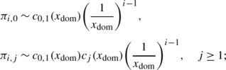
For the singular random walk in case 5, we have the following exact tail asymptotic properties along the x-direction for large i:

• 1. For $x_{b}^{+}<x_{b_{1}}^{+}$,

  $$\pi_{i+1,j} \sim c_{1,j} \biggl( \frac{1}{x_{b}^{+}} \biggr)^{i}\frac {(i+1)^{j-1}}{(j-1)!}; $$

• 2. For $x_{b}^{+}=x_{b_{1}}^{+}$,

  $$\pi_{i+1,j} \sim c_{2,j} \biggl( \frac{1}{x_{b}^{+}} \biggr)^{i}\frac {(i+1)^{j}}{j!}; $$

• 3. For $x_{b}^{+}>x_{b_{1}}^{+}$,

  $$\pi_{i+1,j} \sim c_{3,j} \biggl( \frac{1}{x_{b_{1}}^{+}} \biggr)^{i}. $$

Remark 5.1

All coefficients c _i,j can be explicitly expressed in terms of system parameters, which will be done in Sect. 5.3.

5.2 Along the y-direction

In this case, we can use the standard procedure of the kernel method for non-singular random walks presented in [10]. In the following, we express π ₂(y) in terms of π ₁(x) considering x as a function of y.

First, consider the equation h(x,y)=0. For a fixed y, the two roots are given by

where

$$D(y)=\bigl[p_{0,1}y-(1-p_{0,0})\bigr]^{2}-4(p_{1,0}+p_{1,1}y) (p_{-1,0}+p_{-1,1}y). $$

To locate the two branch points, notice that D(1)>0 and $D ( \frac{1-p_{0,0}}{p_{0,1}} ) <0$, which implies that D(y) has a root (a branch point), denoted by y ₃, between 1 and $\frac{1-p_{0,0}}{p_{0,1}}$. If $p_{0,1}^{2}-4p_{1,1}p_{-1,1}>0$, the other distinct root, denoted by y ₄, of D(x) is greater than $\frac{1-p_{0,0}}{p_{0,1}}$; otherwise this root is smaller than −y ₃. Write

$$D(y) = d \biggl( 1-\frac{y}{y_{3}} \biggr) \biggl( 1-\frac {y}{y_{4}} \biggr), $$

where $d =[p_{0,1}^{2}-4p_{1,1}p_{-1,1}]y_{3}y_{4}$.

For |y|≤1, let

$$x=X_{0}(y)= \begin{cases} X_{-}(y), &\text{if }|X_{-}(y)|\leq|X_{+}(y)|, \\ X_{+}(y), &\text{if }|X_{-}(y)|>|X_{+}(y)|. \end{cases} $$

According to [3], X ₀(y) is analytic everywhere except on the cut [y ₃,y ₄]. Let $P(x,y)=\sum_{i=-1}^{1}\sum_{j=-1}^{1}p_{i,j}x^{i}y^{j}$ $= \frac{h(x,y)}{xy}+1$. It can be shown, either directly or similar to the argument used in [3], that equation P(x,y)=1 for |y|=|x|=1 cannot hold except for x=y=1. Hence, for |y|=1 and y≠1, |X ₀(y)|≠1 since P(X ₀(y),y)=1. It is easy to see that

$$\bigl|X_{0}(-1)\bigr|=\frac{|1-p_{0,0}+p_{0,1}-\sqrt {D(-1)}|}{2|p_{1,0}-p_{1,1}|}. $$

By direct algebra, we obtain |X ₀(−1)|<1. It follows that for |y|=1,y≠1, |X ₀(y)|≤1. This is because if there were y′, |y′|=1, such that |X ₀(y′)|>1, then there would exist y′′, |y′′|=1 and y′′≠1, such that |X ₀(y″)|=1, which is impossible. Since X ₀(y) is analytic on the disk |y|≤1, we obtain that |X ₀(y)|≤1 when |y|≤1 from the maximum modulus principle.

Therefore, we have

$$0=h_{1}\bigl(X_{0}(y),y\bigr)\pi_{1} \bigl(X_{0}(y)\bigr)+h_{2}\bigl(X_{0}(y),y\bigr) \pi_{2}(y)+h_{0}\bigl(X_{0}(y),y\bigr) \pi_{0,0} $$

or

To specify the type of exact tail asymptotics, we need to locate zeros of h ₂(X ₀(y),y). For convenience, let us study the zeros of the polynomial

$$g(y) = \tilde{a}(y)h_{2}\bigl(X_{0}(y),y \bigr)h_{2}\bigl(X_{1}(y),y\bigr) =\tilde{a}(y) \tilde{b}_{2}^{2}(y)-\tilde{b}(y)\tilde{b}_{2}(y) \tilde{a}_{2}(y)+\tilde{c}(y)\tilde{a}_{2}^{2}(y), $$

where X ₁(y) is defined by

$$X_1(y)= \begin{cases} X_{-}(y), &\text{if }|X_{-}(y)| > |X_{+}(y)|, \\ X_{+}(y), &\text{if }|X_{-}(y)| \leq|X_{+}(y)|. \end{cases} $$

Since g(0)=0 and g(1)=0, we only need to solve a polynomial equation of degree 4.

From M _x <0, we know $h_{2}^{\prime}(X_{0}(1),1)=h_{2}^{\prime}(1,1)<0$. It follows that h ₂(X ₀(y),y) has a zero in (1,y ₃] if h ₂(X ₀(y ₃),y ₃)≥0 since h ₂(X ₀(1),1)=0. Denote such a zero by y ^∗. Using the same argument as in Sect. 5.2 of [10], we can show that y ^∗ is the only possible zero of h ₂(X ₀(y),y) whose modulus is in (1,y ₃]. Also, let $\tilde{y}$ be the solution of $X_{0}(y)=x_{b_{1}}^{+}$ in (1,y ₃], where $x_{b_{1}}^{+}$ is given in (2.8) if such a solution exists, otherwise let $\tilde{y}>y_{3}$. Similarly, we assume y ^∗>y ₃ if h ₂(X ₀(y),y) has no zero with its modulus in (1,y ₃]. This convention is simply for convenience of using the minimum function. Finally, let $y_{\mathrm{dom}}=\min(y^{\ast},\tilde{y},y_{3})$ be the dominant singular point of π ₂(y).

Using the Tauberian-like theorem on π ₂(y) as well as on $\pi_{2}^{\prime}(y)$ when $y_{\mathrm{dom}}=y_{3}<\min (y^{\ast},\tilde{y})$, we obtain the tail asymptotics for π _0,j . By a similar argument to that for Theorem 3.1, we can show that ψ _i (y), i≥1, has the same dominant singular point as ψ ₀(y)=π ₂(y) and the tail asymptotics for π _i,j for i≥1.

Theorem 5.2

For the singular random walk in case 5, we have a total of four different types of tail asymptotic properties along the y-direction for large j.

• Type 1: (Exact geometric decay) For $y_{\mathrm{dom}}=\min \{y^{\ast}, \tilde{y}\}<y_{3}$ or $y_{\mathrm{dom}}=\tilde{y}= y^{\ast}=y_{3}$,

  

• Type 2: (Geometric decay multiplied by a factor j ^−1/2) For $y_{\mathrm{dom}}=y_{3}=\min\{y^{\ast},\tilde{y}\}$ and $y^{\ast}\neq\tilde{y}$,

  

  (5.4)
  

  (5.5)

• Type 3: (Geometric decay multiplied by a factor j ^−3/2) For $y_{3}=y_{\mathrm{dom}}<\min\{y^{\ast},\tilde{y}\}$,

  

  (5.6)
  

  (5.7)

• Type 4: (Geometric decay multiplied by a factor j) For $y_{\mathrm{dom}}=y^{\ast}=\tilde{y}<y_{3}$,

  

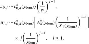
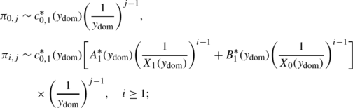
where $c_{0,1}^{\ast}(y_{\mathrm{dom}})$, $c_{0,4}^{\ast}(y_{\mathrm {dom}})$, B ₁(y), A ₁(y) and A ₄(y) are given in Sect. 4 and

Remark 5.2

Coefficients c _0,i , A _i , and B _i are explicitly expressed in terms of system parameters, since they are dependent on the function π ₂(y), which is explicitly determined in this case.

5.3 Determinations of coefficients c _i,j for i=1,2,3, and j≥0

All coefficients c _i,j in Sect. 5.1 can be explicitly expressed in terms of system parameters. For this purpose, we only need to determine π _0,0, π _0,1, and π _0,2. The same method used in Sect. 2.1 can be repeated here.

Since the expression for φ ₀(x) for case 1 is also valid for case 5, we have

π _0,0 is determined according to the normalization condition with the same formula:

$$\pi_{0,0}=\frac{1}{1+t_{1}+t_{2}+t_{3}}, $$

where t ₁ and t ₃ share the same expressions as for case 1, and we have

$$t_{2}=-\mbox{\fontsize{8.9pt}{9pt}\selectfont $\dfrac{a_{1}(1)t_{1}+X_{0}^{\prime}(1) \{ [p_{1,1}^{(1)}+p_{1,0}^{(1)}]-[p_{-1,0}^{(1)}+p_{-1,1}^{(1)}] \} t_{1}+ \{ a_{0}(1)+X_{0}^{\prime}(1) [ p_{1,0}^{(0)}+p_{1,1}^{(0)} ] \} }{\tilde{a}_{2}(1)X_{0}^{\prime}(1)+ \{ [p_{1,1}^{(2)}+p_{0,1}^{(2)}]-[p_{0,-1}^{(2)}+p_{1,-1}^{(2)}] \} }$}. $$

6 Exact tail asymptotics for case 7 and case 8

Case 7 and case 8 are symmetric. Here, we provide details for case 7 only and the corresponding results for case 8 can be easily obtained by symmetry. for case 7, we have

6.1 Along the y-direction

Consider the kernel equation h(x,y)=0. For a fixed y, we find

$$X_{\pm}(y)=-\frac{\tilde{b}(y)}{2\tilde{a}(y)}\pm\sqrt{\frac {\tilde{b}^{2}(y)-4\tilde{a}(y)\tilde{c}(y)}{4\tilde{a}^{2}(y)}}, $$

where D(y)=[p _0,−1−(1−p _0,0)y]²−4(p _1,−1+p _1,0 y)(p _−1,−1+p _−1,0 y).

Let $y_{\tilde{b}}=\frac{p_{0,-1}}{1-p_{0,0}}$. Since D(0)>0, $D(y_{\tilde{b}})<0$ and D(1)>0, D(y) has two zeros, denoted by y ₁ and y ₂, in the interval (0,1). Let x=X ₀(y) be defined in the same way as in Sect. 5.2 and follow a similar argument there to show that |X ₀(y)|≤1 for |y|≥1.

Since X ₀(y) and π ₂(y) are analytic on |y|=1, and π ₁(x) is analytic on |x|=1, near |y|=1 we can write

$$\pi_{2}(y)=\frac{-h_{1}(X_{0}(y),y)\pi _{1}(X_{0}(y))-h_{0}(X_{0}(y),y)\pi_{0,0}}{h_{2}(X_{0}(y),y)}. $$

Since for |y|≥1, |X ₀(y)|≤1, the only possible singular point of π ₂(y) is a zero of h ₂(X ₀(y),y). Therefore, π _0,j has a geometric solution with rate 1/y _dom, where y _dom is the dominant pole of π ₂(y). Using the same argument as in Sect. 5.2 of [10], we can show that y _dom is a simple zero of h ₂(X ₀(y),y) and h ₂(X ₀(y),y) has no other zero on the circle |y|=y _dom.

Now, using the Tauberian-like theorem and a similar argument to that for Theorem 3.1, we have the following tail asymptotic property.

Theorem 6.1

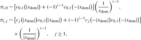
For the singular random walk in case 7, the joint distribution has an exact geometric tail along the y-direction with rate 1/y _dom; i.e. for a fixed i≥0 and for large j,

where

$$C_{0}=\frac{-h_{1}(X_{0}(y_{\mathrm{dom}}),y_{\mathrm{dom}})\pi _{1}(X_{0}(y_{\mathrm{dom}}))-h_{0}(X_{0}(y_{\mathrm {dom}}),y_{\mathrm{dom}})\pi_{0,0}}{h_{2}^{\prime} (X_{0}(y_{\mathrm{dom}}),y_{\mathrm{dom}})X_{0}^{\prime}(y_{\mathrm{dom}})}, $$

and $A=\frac{-C_{0}b_{1}(y_{\mathrm{dom}})}{c(y_{\mathrm{dom}})}$.

Remark 6.1

C ₀ can expressed explicitly in terms of the unknown function π ₁(x). However, it cannot be explicitly expressed in terms of system parameters unless further information about the unknown function becomes available.

6.2 Along the x-direction

Once again, consider the kernel equation h(x,y)=0. For a fixed x, the unique y is given by

$$y=Y(x)=\frac{c(x)}{-b(x)}. $$

Near the unit circle |x|=1, all Y(x), π ₁(x) and π ₂(Y(x)) are analytic. Hence, we have, near |x|=1,

$$\pi_{1}(x)=\frac{-h_{2}(x,Y(x))\pi_{2}(Y(x))-h_{0}(x,Y(x))\pi _{0,0}}{h_{1}(x,Y_{0}(x))}, $$

which, in fact, holds for ε′<|x|<R′, where 0<ε′<1 and R′ is the dominant singular point of π ₁(x). Note that π ₂(Y(x)) is analytic if |Y(x)|<y _dom, where y _dom is the pole of π ₂(y).

We first notice that b(x) has two zeros $x_{b}^{\pm}$ given by (2.9). We then consider the equation Y(x)=y ^∗, where y ^∗ is the zero of h ₂(X ₀(y),y) in (1,∞), or c(x)+y ^∗ b(x)=0. Since c(0)+y ^∗ b(0)>0 and c(1)+y ^∗ b(1)<c(1)+b(1)<0, Y(x)=y ^∗ has a unique root, denoted by $\tilde{x}$, in $(1, x_{b}^{+})$. If $\tilde{x}$ ≠X ₀(y ^∗), we have

$$\lim_{x\rightarrow\tilde{x}}\frac {h_{2}(x,Y(x))}{h_{2}(X_{0}(Y(x)),Y(x))}=\infty, $$

which indicates that $\tilde{x}$ is a potential pole of π ₁(x) since

Note that $x_{b}^{+}$ is not a singular point of π ₁(x) since X ₀(Y(x))<1 when Y(x)>1. Let x ^∗ be the zero of h ₁(x,Y(x)). Using elementary algebra, we can show that x ^∗ is positive and simple, and h ₁(x,Y(x)) has no other zeros on the circle |x|=x ^∗.

Again, by using the Tauberian-like theorem and a similar argument to that for Theorem 3.1, we have the following tail asymptotic property.

Theorem 6.2

For the singular random walk in case 7, the joint distribution has the following exact tail asymptotic properties along the x-direction; i.e. for a fixed j and for large i,

• 1. (Exact geometric decay) If $x^{\ast}\neq\tilde{x}$, then π _i,j has an exact geometric tail decay with rate equal to $\max\{\frac{1}{x^{\ast}},\frac{1}{\tilde{x}} \}$, or

  $$\pi_{i,j} \sim c_{1,j} \biggl( \frac{1}{x_{\mathrm{dom}}} \biggr)^{i-1}, $$

  where $x_{\mathrm{dom}} = \min\{x^{*},\tilde{x}\}$ and c _1,j are constants independent of i and j.

• 2. (Geometric multiplied by a factor of i) If $x^{\ast}=\tilde{x}$, then π _i,j has a geometric tail decay with rate x ^∗ multiplied by a prefactor i, or

  $$\pi_{i,j} \sim c^*_{1,j} (i-1) \biggl( \frac{1}{x_{\mathrm{dom}}} \biggr)^{i-1}, $$

  where $x_{\mathrm{dom}} = x^{*}=\tilde{x}$ and $c_{j,0}^{*}$ are constants independent of i.

Remark 6.2

In the above theorem, we can explicitly express c _1,j and $c^{*}_{1,j}$ in terms of c _1,0 and $c_{1,0}^{*}$, respectively, as for case 4. However, c _1,0 and $c_{1,0}^{*}$ are dependent on the unknown functions π ₂(y) and π ₁(x), respectively. Therefore, they cannot be explicitly expressed in terms of system parameters unless further information about the unknown functions becomes available.

7 Concluding remarks

In this paper, we considered exact tail asymptotics of stationary probabilities for singular random walks in the quarter plane. This brings to a closure the study on exact tail asymptotics of the joint distribution along a coordinate direction and also of the two marginal distributions. For a stable random walk in the quarter plane with M≠0, there are a total of four possible types of exact tail asymptotics along a coordinate direction and of a marginal distribution for all cases, non-singular or singular, except for singular cases 5 and 6. They are exact geometric and geometric multiplied by a pre-factor of n ^−1/2, n ^−3/2 and n, respectively. For case 6, for a fixed j>0 and large i, π _i,j has a new type of exact tail asymptotic. A symmetric property holds for case 7 as well.

Another note is that all asymptotic coefficients can be explicitly expressed in terms of system parameters for following cases: case 1, case 2, case 5, and case 6. For other cases, coefficients depend on functions that cannot be explicitly expressed using the analysis provided in the paper.

In this paper, we only considered random walks in the quarter plane, which are allowed to move to neighborhood states, that is, jumps are not allowed. For a random walk in the quarter plane which allows jumps, or for a random walk in a higher dimensional space, many interesting problems are still open.

References

Abate, J., Whitt, W.: Asymptotics for M/G/1 low-priority waiting-time tail probabilities. Queueing Syst. 25, 173–233 (1997)
Bender, E.: Asymptotic methods in enumeration. SIAM Rev. 16, 485–513 (1974)
Fayolle, G., Iasnogorodski, R., Malyshev, V.: Random Walks in the Quarter-Plane. Springer, New York (1999)
Flajolet, P., Odlyzko, A.: Singularity analysis of generating functions. SIAM J. Discrete Math. 3, 216–240 (1990)
Guillemin, F., Simonian, A.: Asymptotics for random walks in the quarter plane with queueing applications. In: Skogseid, A., Fasano, V. (eds.) Statistical Mechanics and Random Walks: Principles, Processes and Applications, pp. 389–420. Nova Publ., New York (2011)
He, Q., Li, H., Zhao, Y.Q.: Light-tailed behaviour in QBD process with countably many phases. Stoch. Models 25, 50–75 (2009)
Kobayashi, M., Miyazawa, M.: Tail asymptotics of the stationary distribution of a two dimensional reflecting random walk with unbounded upward jumps (2011, submitted)
Li, H., Zhao, Y.Q.: Exact tail asymptotics in a priority queue—characterizations of the preemptive model. Queueing Syst. 63, 355–381 (2009)
Li, H., Zhao, Y.Q.: Tail asymptotics for a generalized two-demand queueing model—a kernel method. Queueing Syst. 69, 77–100 (2011)
Li, H., Zhao, Y.Q.: A kernel method for exact tail asymptotics—random walks in the quarter plane (2011). Under revision
Miyazawa, M.: Tail decay rates in double QBD processes and related reflected random walks. Math. Oper. Res. 34, 547–575 (2009)
Miyazawa, M.: Light tail asymptotics in multidimensional reflecting processes for queueing networks. Top (2011). doi:10.1007/s11750-011-0179-7
Author information
Authors and Affiliations
Corresponding author
Rights and permissions
About this article
Cite this article
Li, H., Tavakoli, J. & Zhao, Y.Q. Analysis of exact tail asymptotics for singular random walks in the quarter plane. Queueing Syst 74, 151–179 (2013). https://doi.org/10.1007/s11134-012-9321-y
Received:
Revised:
Published:
Issue Date:
DOI: https://doi.org/10.1007/s11134-012-9321-y
Keywords
- Singular random walks in the quarter plane
- Generating functions
- Stationary probabilities
- Kernel method
- Asymptotic analysis
- Dominant singularity
- Exact tail asymptotics