Dynamic parameter sensitivity in numerical modelling of cyclone-induced waves: a multi-look approach using advanced meta-modelling techniques

Abstract

The knowledge and prediction of cyclones as well as wave models experienced significant improvements in this last decade, opening the perspective of a better understanding of the wave sensitivity to the cyclone characteristics (e.g. track angle of approach θ, forward speed V _f, radius of maximum wind R _m, landfall position x _o, etc.). Physically, waves are strongly linked to the time-varying evolution of the relative cyclone position. Thus, even assuming the main cyclone characteristics to be stationary, exploring the role played by each of them should necessarily be conducted in a dynamic manner. This problem is investigated using the advanced statistical tools of variance-based global sensitivity analysis (VBSA) in different ways to provide an overall view of wave height sensitivity to cyclone characteristics: (1) step-by-step: by computing the time series of sensitivity measures; (2) aggregated: by summarising the time-varying information into a single sensitivity indicator; (3). mode-based: by studying the sensitivity with respect to the occurrence of specific temporal patterns (e.g. up-down translation of the overall series). Yet, applying this multi-look dynamic sensitivity analysis faces two major difficulties: (1) VBSA requires a large number of simulations (typically > 10,000), which appears to be incompatible with the large computation time cost of numerical codes (>several hours for a single run); (2) integrating the time dimension imposes to process a large amount of information via vectors of large size (e.g. series of significant wave height H _S discretised over several hundreds of time steps). In this study, we propose a joint procedure combining kriging meta-modelling (to overcome the 1st issue) and principal component analysis techniques (to overcome the 2nd issue by summarising the time information into a limited number of components). The applicability of this strategy is tested and demonstrated on a real case (Sainte-Suzanne city, located at Reunion Island) using a set of 100 cyclone-induced H _S series, each of them being computed for different scenarios of cyclone characteristics, i.e. using only 100 long-running simulations. The key role of R _m over the whole evolution of H _S is shown by means of the aggregated option, with a more specific influence in the vicinity of Sainte-Suzanne (when the cyclone eye is located less than 200 km away from the site) as highlighted by the step-by-step option. The step-by-step option also highlights the influence of the landfall position on the H _S peak reached in strong interaction with θ and R _m. Finally, the role of V _f in the occurrence of a turning point marking a shift near landfall between regimes of low-to-high H _S values is also identified. The above results provide guidelines for future research efforts on cyclone characteristics prediction.

1 Introduction

Tropical cyclones are among the world’s most destructive natural disasters that devastate properties and cause loss of life (e.g. Terry and Gienko 2010; Diamond et al. 2012). It can produce not only extremely powerful winds and heavy rainfall, but also large atmospheric storm surge and waves, which can generate an additional increase in the water level at the coast (wave setup) as well as overtopping over coastal defences. Storm-generated waves can propagate very far away from the cyclone eye until reaching nearshore regions and are affected by the characteristics (denoted x) of the cyclone approaching the coastline. To a first order, these characteristics basically correspond to the track angle of approach θ, the landfall position x _o (or the cyclone eye position closest to the studied site), the forward speed V _f, the radius of maximum winds R _m, the maximum wind speed V _m and the shift around the central pressure δP. These are the primary inputs for generating regional databases of synthetic cyclone scenarios, which are necessary for regional flooding and coastal hazard studies (Kennedy et al. 2012; Resio et al. 2009) and more specifically for probabilistic hurricane risk evaluation (Irish et al. 2011; Niedoroda et al. 2008, 2010). Depending on these characteristics, waves and atmospheric storm surge at the coast can significantly vary. For instance, Irish et al. (2009) and Song et al. (2012) showed the effect of varying the cyclone size, the intensity and the track on the peak magnitude and location of the atmospheric surge variation as a function of the alongshore distance from landfall position. Getting better insight in the relative contributions of each cyclone parameter is of interest:

• To improve predictions by identifying on which parameters, the characterisation effort should primarily be focused on;

• To set up flooding early-warning systems as well as scenarios of forcing conditions as inputs of risk assessment;

• To diagnose model structure (a set of parameters represents a specific process assumed to reflect the real world system under study);

• To support model calibration (to understand which periods of a time series are most helpful in identifying a specific group of parameters).

However, the aforementioned sensitivity studies mainly focus on storm surges and to the authors’ best knowledge, only a few address the temporal evolution of wave characteristics. Yet, cyclone-induced waves may have a primordial importance regarding marine inundation issues, especially for volcanic islands like Reunion Island (south-west Indian Ocean Basin) where the absence of continental shelf and the steep slopes limits the generation of high atmospheric storm surge but increases the potential impact of high waves (Kennedy et al. 2012). Besides, from a methodological perspective, the question of sensitivity is primarily addressed by varying in turn the values of the parameters while keeping the others constant, i.e. by using local sensitivity approaches (see a review by Iooss and Lemaître 2015): these have shown strong limitations as extensively discussed by Saltelli and Annoni (2010). Best practices advocate to preferably address the problem in a global manner using for instance variance-based global sensitivity analysis (VBSA) (Saltelli et al. 2008) whose applicability was demonstrated by a large variety of application cases in different domains (hydrological modelling: Rousseau et al. (2012); landslide modelling: Rohmer and Foerster (2011); marine flooding in a climate change context: Le Cozannet et al. (2015), etc.).

Yet, conducting this type of analysis for cyclone-induced wave modelling faces two major difficulties: (1) quantifying the sensitivity measures typically requires a large number of model runs (of the order of several thousands), whereas the computational requirements of the model (with typical computation time cost of the order of several hours for a single run) usually limit the number of runs that can be made; (2) the processes vary over space and time implying to consider functional (i.e. time varying) variables of interest. A typical output can be the evolution of the significant wave height H _S as a function of time or equivalently as a function of the relative cyclone position (denoted s) defined as the distance between the cyclone eye and the cyclone landfall position x _o at a given time instant (s being negative before landfall and positive after landfall). In the following, we use the generic term “series” to designate both quantities (either time- or space-dependent) and we preferably concentrate on the latter case.

Regarding the first issue (computational time), this can be overcome by means of a meta-model (also called surrogate or proxy, see an introduction by Storlie et al. 2009). A meta-model is a function, which aims at reproducing the behaviour of the “true” model in the domain of model input parameters (here the characteristic feature of the cyclone track). It is constructed using a few computer experiments (i.e. a limited number of time-consuming simulations, typically of the order of 50–100). Once its accuracy is validated (i.e. the low level of meta-model error is demonstrated), it allows estimating the model responses with a negligible computation time (few seconds for any new inputs’ configuration). For instance, Jia et al. (2015) approximated storm surge responses by means of kriging-type meta-models in combination of principal component analysis to handle the temporal character of the response.

Second, the problem of dynamic sensitivity analysis has not a unique answer (as discussed by proposed by Campbell et al. (2006)) and can be looked in different ways (i.e. “one problem, multiple looks”):

• Step-by-step: the objective is to identify the most dominant parameters given specific time instants or intervals. This can be done by analysing the sensitivity for each relative cyclone position separately;

• Aggregated sensitivity indicator: the objective is to summarise the overall temporal (space) information on sensitivity in a single indicator. This can be done using an aggregated sensitivity index as the one proposed by Gamboa et al. (2014);

• Mode-based: the objective is to identify the characteristics which can induce specific functional patterns. In other words, the questions of primary interest are: What shifts the evolution up or down? What makes a possible peak wider or narrower? What reverses the evolution? What accelerates the behaviour? This can be done by extracting the dominant modes of time/space evolution, i.e. the focus is on the overall shapes/form and key structures of the series as originally proposed by Campbell et al. (2006).

Applying these different options can bring complementary information on dynamic sensitivity analysis. In this sense, it can broaden the perspective on each parameter’s role and allow gaining deeper insights in their impact in order to refine decision-making with respect to the four aforementioned issues (prediction improvement, risk scenarios, model calibration and structure).

In this context, the objective of the present study is to perform dynamic sensitivity analysis by following the different modes in order to detect the dominant parameters in the cyclone-induced wave characteristics evolution. We focused on the evolution of the significant wave height H _S versus the relative cyclone position s. In a first section, we describe the motivating application case of Sainte-Suzanne city located at Reunion Island, the grid experiment (100 simulations) and the wave model set-up and validation. To overcome the computational issues, a meta-modelling-based approach is used. In order to facilitate the processing and manipulation of the high-dimensional H _S signal, the meta-model is combined with dimension reduction techniques following the strategies described by Jia et al. (2015) and Rohmer (2014) for time-varying variables. These statistical methods are described in Sect. 3. Finally, we perform the multi-look sensitivity analysis and discuss the results (Sect. 4).

2 Cyclone-induced wave modelling

In this section, we describe in turn the motivating case study used for demonstrating the applicability of the proposed statistical methods (Sect. 2.1), the assumptions made to generate the 100 scenarios with varying cyclone characteristics (Sect. 2.2), and the modelling scheme used to simulate the cyclone-induced waves and the output H_s series at Sainte-Suzanne (Sect. 2.3).

2.1 Description of the case study

Reunion Island is a French Overseas Department located east of Madagascar (see location in Fig. 1a). Due to the mountainous nature of the island, 80 % of the population is concentrated near the coastline, thereby resulting in high vulnerability of these coastal territories to tropical cyclones. The island is exposed to three dominant wave regimes as described by Cazes-Duvat and Paskoff (2004) as well as Lecacheux et al. (2012): trade-wind waves, southern waves and cyclonic waves. Among these regimes, cyclonic waves are the most energetic events and occur only a few days a year between November and March. Cyclone tracks often follow a south-westward trajectory: they usually come from the north-east of Reunion and then continue their course northwards or, less frequently, southwards from the island. Thus, they affect mainly the northern and eastern parts of the island. The lack of continental shelf around the island (cf. Fig. 1b) increases the potential impact of waves that are not dissipated before reaching the coast (except in the reef zones). On the contrary, it reduces the generation of atmospheric storm surges that are essentially due to the inverse barometer effect and then remain localised near the cyclone eye. Even if atmospheric storm surges hardly generate marine inundation by overflowing (the coastal topography being quite high), they may facilitate wave overtopping and then cannot be neglected. In the past decade, seven cyclones passed within 200 km of Réunion Island (see some historical tracks in Fig. 2a).

Fig. 1

a Location of Reunion Island and origin of the last 18 systems affecting the island of the investigated site of Sainte-Suzanne city (map extracted from Climatic Atlas of Météo-France—French national meteorological service, Jumeaux et al. 2011); b bathymetry around Reunion Island and locations of the point of extraction of H _S series from numerical simulations in front of Sainte-Suzanne and the RN4 buoy used for the wave model validation

Fig. 2

a Seven historical tracks selected in the region of Reunion Island, b pseudo-historical tracks obtained by translating the original track relative to the centre of Reunion Island, c example of translation for cyclone pseudo-Giovanna for two opposite landfall positions x ₀

In the present study, we focus on Sainte-Suzanne city, located along a pebble coast in the north-east part of the island (see Fig. 1b). It is a town of 22,000 inhabitants, surrounded by river Sainte-Suzanne and exposed to high cyclonic waves. During the last century, it has been regularly impacted by cyclone-induced inundations, notably due to wave overtopping. For example, the waves generated by cyclones Gamede (2007) and Dina (2002) induced a considerable inundation of the seafront as well as the projection of heavy pebbles (Chateauminois et al. 2014).

2.2 Setting up the simulation scenarios

In this study, we decided to focus on the six main cyclone characteristics and we made the choice for them to remain constant over time (i.e. they remain constant along the cyclone track).

Three parameters describe the intensity, the size and the shape of the cyclone:

• the maximum wind speed V _m;

• the radius of maximum winds R _m, namely the distance from the cyclone eye at which the maximum wind intensity is reached;

• the shift around the central pressure δP. Here, we consider that a mean central pressure P _c can be associated with the maximum wind speed V _m based on the cyclone best-track database established by Météo-France (French national meteorological service) RSMC (Regional Specialised Meteorological Center¹) at Reunion Island by following the climatology for south-west Indian Ocean basin. Making vary P _c influences the shape of the cyclone wind profile whose energy is more or less concentrated near the radius of maximum wind (see Sect. 2.3).

Three parameters enable to characterise the cyclone track:

• the forward speed V _f, defined as the translation speed of the cyclone eye;

• the track angle θ, which is the angle of approach of the cyclone in the vicinity of the studied site. Following Kennedy et al. (2012) and Jia and Taflanidis (2013), we accounted for the variability of the track prior to landfall through an appropriate selection of a limited number of historical cyclone tracks, so that important anticipated variations, based on historical data, are efficiently described. In this study, we selected seven historical tracks in the area of interest covering a broad range of cyclone angles of approach θ (from ~5° to ~175°), hence covering both NE and NO quadrants, in consistency with the track climatology (see Fig. 2a). Then, we translated them so that they cross the centre of Reunion Island. Those final tracks are termed “pseudo-historical” (See Fig. 2b).

• the landfall position x _o, that both characterise the minimum distance and the relative position of the track to the studied site. Basically, we translate the selected track by factor x _o orthogonally to the direction defined by the angle of approach. It enables to consider cyclones passing both west and east (or north and south) of the site at different distances (See Fig. 2c).

Each parameter can vary in a range consistent with the climatology established for south-west Indian Ocean basin based on Météo-France Réunion RSMC cyclone best-track database whose lower and upper bounds are described in Table 1. For the landfall position x ₀, we decided to consider only cyclones passing very close to the island (<100 km) and so that (1) the studied site is in the main direction of wave forward travel and (2) the scenarios are likely to generate overtopping due to the combination of local atmospheric storm surge and waves. In total, five continuous input parameters are accounted for. Since our primary purpose is to explore the influence of cyclone characteristics using synthetic cyclone scenarios (instead of reproducing with high fidelity past historical cyclones), a commonly used assumption is made regarding the uncertainty on the continuous cyclone characteristics: they are assumed to follow a uniform probabilistic law. A possible option to refine this assumption would take advantage of the long-term cyclonic risk for Reunion Island to infer the underlying probability distributions. A parameter of discrete nature is accounted for, namely the scenario of the cyclone track angle θ (ranging from 5° for pseudo-Gael case to 175° or pseudo-Bansi case, see Fig. 2): it is selected among discrete values {5°, 30°, 60°, 90°, 120°, 150°, 175°}. We take advantage of the pieces of information provided by Fig. 1A, namely that values between 5° and 90° have higher frequency, i.e. cyclones coming from NE have higher frequency: for this parameter, we assume that the discrete probabilistic law is not uniform but with 72 % frequency occurrence for values from 5° to 90°.

Table 1 Six cyclone characteristics and associated ranges of variation

2.3 Numerical modelling strategy and validation

2.3.1 Parametric cyclonic winds model

The use of wave models requires the reconstitution of a two-dimensional surface wind input over the entire course of the storm. Here, we use the parametric wind model of Holland (1980). In the southern hemisphere, cyclonic winds follow a circular flow in clockwise direction towards the storm centre. For each scenario, the track is interpolated every hour and the two-dimensional wind fields are calculated with a resolution of 0.1°. The radial wind profile (V _r ) depending on the distance from the eye (r) is estimated with Eq. 1:

$$V_{r} = \sqrt {B\frac{{(P_{n} - P_{c} )}}{{\rho_{a} }} \times \left(\frac{{R_{m} }}{r}\right)^{B} \times \exp \left( - \left(\frac{{R_{m} }}{r}\right)^{B}\right) + \frac{{r^{2} f^{2} }}{4}} - \frac{rf}{2}\quad {\text{with}}\quad B \approx \frac{{V_{m}^{2} \rho_{a} e}}{{(P_{n} - P_{c} )}}$$

(1)

where f is the Coriolis force, ρ _a the air density (~1.15 kg m⁻³), V _m the maximum wind speed, R _m the radius of maximum wind, P _c the central pressure and P _n the environmental pressure (~1010 hPa in this region). The influence of parameters V _m , R _m and δP on the wind profile is illustrated on Fig. 3. While an increase of R _m leads to a widening of the wind profile over hundreds of kilometres and, in a way, an expansion of the fetch (surface over which the wind blows), an increase of V _m accentuates the amplitude of the profile in the vicinity of R _m . A negative perturbation of δP (the shift around the central pressure P _c ) leads to an increase of the dispersion of wind profile (but to a lesser extent than R _m ), but without affecting the maximum wind amplitude.

Fig. 3

Comparison of parametric cyclonic wind profiles calculated with the formula of Holland (1980) for different sets of parameters

It should be noted that the aforedescribed model remains a simplification since cyclonic wind speed and shape are usually not symmetric (Shapiro 1983; Wang and Holland 1996): the shape of historical cyclones is usually corrected based on observations of radial extents of 34–50–64 kt winds in the four quadrants (Xie et al. 2006). But to the authors’ best knowledge, no consensus exists in the literature on how these contributions could be integrated into parametric models. Besides, the correction with observations of 34–50–64 kt winds cannot be applied in our case. Therefore, the symmetrical assumption is chosen to be kept.

2.3.2 Wave fields modelling, validation and description

The wave model (see Fig. 4a) is a combination of a two-way nested Wavewatch 3 modelling framework (Tolman 2014; hereinafter denoted WW3) enabling the offshore waves generation and propagation to Reunion Island coastlines. The version 4.18 of WW3 is used with the source term package described by Ardhuin et al. (2010) and a discretisation in 32 frequencies and 36 directions. The first grid R1 covers a large part of the south Indian Ocean with a regular resolution of 0.1° while R2, centred on Reunion island, is composed of finite elements whose resolution reach about 300 m at the coast. For R2, the global time step is set to 200 s and the maximum CFL time steps to 50 s (spatial advection) and 20 s (angular advection). The computational time of the whole chain is about half an hour to simulate 1 day on 24 central processing unit (CPU). The bathymetric data used come from ETOPO1 with a spatial resolution of 1 min (Amante and Eakins 2009) as well as the bathymetric measurements from the SHOM (French Naval Hydrographic and Oceanographic Service) in the vicinity of the island. For each simulated cyclone, the time series of H _S (with 10-min-frequency) are extracted from the coastal grid at 50 m depth in front of the site of Sainte-Suzanne.

Fig. 4

a Boundaries of the two WW3 grids (R1 and R2) and map of H _S (colour shading) and Tp (white contours) computed for cyclone Bejisa on 2, January at 0 h UTC using the south Indian Ocean grid. Bejisa’s track and forward direction are symbolised by the red line and arrows. b zoom on the core of the wave field and indications on wave direction (arrows). c comparison between simulated (lines) and measured (dots) H _S and T _p at NorteckMed RN4 buoy

An example of wave field simulated with the WW3 modelling framework for cyclone Bejisa (January 2014) is given in Fig. 4a. The associated-wind field was calculated (1) by applying the same formula used for the synthetic scenarios and the parameters extracted from the re-analysed cyclone best-track (Météo-France Réunion RSMC cyclone database) and (2) by merging the previous cyclonic wind field with environmental wind fields of GFS analysis operated by NOAA/NCEP. This process enables to obtain more realistic waves before the cyclone landfall by taking into account background non-cyclonic waves.

The simulated wave field (Fig. 4a, b) exhibits (1) a circular outward pattern with large waves near the radius of maximum wind that propagate far away from the cyclone eye and (2) a calmer zone in the neighbourhood of the eye whose size is controlled by the extension of R _m. The amount of energy transferred from the wind to the waves and then the height of generated waves, is mainly controlled by parameters V _m and R _m that influence, respectively, the intensity and the extent over which the wind blows (fetch). Yet, the translation speed also plays an important role in the wave generation zone and may modify the aforementioned symmetrical circular pattern (Liu et al. 2007; Phadke et al. 2003):

• In the left-forward quadrant, the coincidence of the forward speed with the wave propagation direction increases the transfer of energy from wind to growing waves by prolonging the wind action and then induces the generation of higher and longer waves. While the forward speed remains lower than the induced wave’s group velocity, H _S monotonically increases with the translation speed. However, in the event of a cyclone travelling faster than the generated waves, the duration of the wind action is reduced and decreases the transfer of energy and the related wave heights;

• In the other quadrant, the locally generated waves are lower and shorter due to the limited fetch and duration as the cyclone moves on the opposite direction of wave generation zone.

It should be noticed that the zone of influence of the forward speed exceeds the wave propagation zone and affects the wave pattern far away from the cyclone eye. When V _f is much below the dominant wave group velocity, generated waves can propagate far forward the cyclone centre and the wave field is more extended ahead. On the other hand, for fast moving cyclones, if the forward speed is similar or faster than the wave propagation speed, waves remain close or lag behind the core of the cyclone. Then, the wave field seems to be more extended backward.

The wave parameters simulated for cyclone Bejisa were compared with the measurements of the AWAC wave gauge deployed by NortekMed at RN4 station (located at 20°51,767′S and 55°27,055′E, see Fig. 1a, b). The comparison of significant wave heights and peak periods is considered satisfactory (Fig. 4c) despite discrepancies near the peak of wave heights, which are possibly related to the simplified symmetrical shape of cyclonic winds: improving this issue is out of the scope of the present study.

2.3.3 Computation of the H_S series

Using the aforedescribed modelling strategy, the H _S series as a function of the relative cyclone position s (recall that s is negative before landfall and positive after landfall) are computed for the Sainte-Suzanne case considering a hundred of randomly generated configurations for the cyclone characteristics (Sect. 2). The random sampling of the continuous parameters is performed using the Latin hypercube sampling (LHS) method (McKay et al. 1979) in combination with the “maxi–min” space filling design criterion (Koehler and Owen 1996) in order to optimise the exploration of the input domain space, while minimising the number of simulations. The sampling of cyclone track angle θ (parameter of discrete nature) is done by traditional sampling with replacement.

The computation of the 100 scenarios with the modelling chain described above took about 8 days with 24 CPU. Figure 5 provides the mean and the quantiles at 95 and 75 %. The simulation scenarios cover a large broad of H _S peak values up to ~17.44 m. As illustrated by the two scenarios of largest H _S peaks (scenario N°48 and N°92 depicted in red in Fig. 5), the series of H _S are not necessarily symmetrical with respect to s = 0 (landfall) and the peak values of H _S do not necessarily correspond to s = 0 since some translated tracks may pass on the opposite side of the island relative to Sainte-Suzanne (the maximum wave height occurring then before landfall).

Fig. 5

Set of H _S as a function of the cyclone relative position s considering the 100 scenarios generated by varying the cyclone characteristics’ values using the assumptions described in Table 1

3 Statistical methods

This section addresses the issue of dealing with functional outputs for sensitivity analysis of long-running models. The term “functional” is used to refer to variables, which are not scalar (i.e. they do not take a single value), but they are complex functions of time or space (or both). In this study, we restrict the analysis to the case where the output is a function of one variable (here the relative cyclone position s) but this analysis can be extended to account for space-dependent (e.g. Jia and Taflanidis (2013)) and space–time variables (e.g. Antoniadis et al. 2012). The proposed strategy (described in Sect. 3.1) relies on the one proposed by different authors (e.g. Jia et al. 2015; Rohmer 2014) for handling time-varying outputs. Some adaptations of the methods were necessary to overcome the difficulties in the considered case, namely: (1) handling scenario-like input parameter, aka categorical: in our case, this corresponds to the limited number of scenarios of cyclone track angles θ; (2) accounting for the meta-model error (the uncertainty introduced by replacing the true numerical code by an approximation) in the presentation of the results.

3.1 Strategy description

The whole strategy aims at identifying the most dominant cyclone characteristics regarding H _S uncertainty given the relative cyclone position s. This is done by relying on VBSA and by adopting different perspectives for conducting this analysis in a dynamic manner (Sect. 3.2). Since the simulator f for wave modelling is of high computation time cost (several hours), a necessary procedure aims at approximating the series of H _S as a mathematical function of the cyclone characteristics x. This function named meta-model should be costless to evaluate and should be constructed using a limited number of x configurations (typically 50–100) as generated in Sect. 2.3. We chose to focus on meta-models of type kriging (Sect. 3.4). Since the model output is of functional nature, a preliminary step aims at summarising the functional information using a limited number of components (typically of the order of 10) based on basis set expansion techniques (Sect. 3.3). Once the quality of the approximation (Sect. 3.5) has been validated, the kriging meta-model can replace the simulator for conducting dynamic VBSA.

3.2 Variance-based sensitivity analysis

The basic concepts of VBSA are first briefly introduced considering a scalar output h. For a more complete introduction, the interested reader can refer to Saltelli et al. (2008) and references therein. VBSA aims at determining the part of the total unconditional variance Var(h) of the output h resulting from the variation of each the m input independent random variable X _i . This analysis relies on the functional analysis of variance (ANOVA) decomposition of f based on which two sensitivity indices ranging between 0 and 1 (aka Sobol’ indices), namely the main and total effects (respectively, denoted $S_{i}$ and $S_{Ti}$), can be defined as follows:

$$S_{i} = \frac{{\text{Var}\left[ {\text{E}\left( {\left. h \right|X_{i} } \right)} \right]}}{{\text{Var}(h)}},\begin{array}{*{20}c} {} & {S_{Ti} = 1 - \frac{{\text{Var}\left[ {\text{E}\left( {\left. h \right|X_{ - i} } \right)} \right]}}{{\text{Var}(h)}}} \\ \end{array}$$

(2)

where X _-i  = (X ₁ ,…, X _i−1 , X _i+1 ,…, X _m ). The main effect S _i can be interpreted as the expected amount of Var(h) (i.e. representing the uncertainty in h) that would be reduced if it was possible to learn the true value of X _i. This index provides a measure of importance useful to rank in terms of importance the different input parameters (Saltelli et al. 2008). The total index $S_{Ti}$ corresponds to the fraction of the uncertainty in Y that can be attributed to X _i and its interactions with all other input parameters. $S_{Ti} \approx 0$ means that the input factor X _i has little effect so that X _i can be fixed at any value over its uncertainty range (Saltelli et al. 2008).

Different algorithms are available for the estimation of the Sobol’ indices (an extensive introduction is provided by Saltelli et al. (2008: chapter 4)). In the present study, we used the algorithm proposed by Jansen (1999) and Saltelli et al. (2010). The common feature of all those estimation algorithms is their cost in terms of number of required simulations (typically of several thousands). This can be overcome using meta-modelling techniques as described in Sect. 3.4. As underlined in the introduction, when it comes to dynamic sensitivity analysis, i.e. dedicated to functional outputs, different options are available in the literature:

• 1. Step-by-step option: This can be done at each time step. VBSA is then re-conducted N times, N being the number of time discretisation of the time series. Though this is the simplest approach, this may also become intractable for long series (N exceeding several hundreds), and it may introduce a high level of redundancy, because it neglects the strong relationship between output values from successive steps;

• 2. Aggregated option: This can be done by relying on aggregated sensitivity measures like the one proposed by Gamboa et al. (2014), which basically averages all the sensitivity indices weighted by the variance of the functional output. This is detailed in “Appendix 1”;

• 3. Mode-based option: This consists in the reduction of the dimensionality of the output quantity N by expanding it in an appropriate and new functional coordinate system described by a limited number d (d << N) of new basis functions $\varphi_{j} (s)$, with j = 1, …, d: these correspond to the main modes of variation. Further details are provided below in Sect. 3.3. This procedure is then followed by VBSA for the coefficients of the expansion h _j. For instance, if the expansion coefficients h ₁ for the first basis function $\varphi_{1}$ are sensitive to a particular input parameter, this means that this parameter is important in producing the type of behaviour described by $\varphi_{1}$.

3.3 Basis set expansion

In this section, we introduce the basic concepts for processing functional variables in order to make feasible the dynamic sensitivity analysis. Formally, consider a set of n ₀ functional model outputs, $H_{S}^{(i)}$ (with i = 1,…, n ₀) and discretised into N steps.

In the Reunion Island case, the set of functional model outputs correspond to n ₀ = 100 vectors of H _S with N = 500 (number of relative cyclone positions). The objective of the basis set expansion is then to project the set of curves onto an appropriate functional coordinate system, i.e. in terms of some basis functions of s, denoted $\varphi_{k} (s)$ (with k = 1,…, d) whose dimension d << 500 so that the new functions $\varphi_{k} (s)$ describe the key features of the evolution of the calculated H _S, i.e. their dominant modes of variations. The basis set expansion of the set of centred temporal curves $H_{S}^{C} (s)$ reads as Eq. (3):

$$H_{S}^{C,(i)} (s) = H_{S}^{(i)} (s) - \bar{H}_{S} (s) \approx \sum\limits_{k = 1}^{d} {h_{ik} \varphi_{k} (s)}$$

(3)

where the mean temporal function $\bar{H}_{S}$ is computed as the mean of H _S at each discretisation step s. The scalar expansion coefficients h _ik indicate the “weight” (contribution) of the kth basis function (k = 1,…, d) in the approximation of the ith considered curve (i = 1,…, n ₀). Usually, the dimension d is chosen so that most information is concentrated in the d first basis functions. For instance, a criterion based on the explained variance in the set of curves can be used by selecting at a minimum level of, let say, 99.9 % (see further details in “Appendix 3”).

The basis functions $\varphi_{k}$ can be of various forms, such as pre-defined Legendre polynomials, trigonometric functions, Haar functions, or wavelet bases, etc. (Ramsay and Silverman 2005). The disadvantage is to give beforehand an idea of the modes of variations. Alternatives are adaptive basis functions, which determine the basis functions from the data. The classical data-driven method is the multivariate principal component analysis, denoted PCA (Jolliffe 2002), which can be applied to the functional model outputs viewed as vectors of finite dimension. Further details are provided in “Appendix 3”. Another attractive feature is the ability to interpret these new basis functions as perturbations from the mean temporal function, i.e. deviations from the “average” behaviour following the recommendations of Campbell et al. (2006). In the following, we will focus on this approach.

3.4 Kriging-based meta-modelling

Once the functional information has been summarised using Eq. 3, the basic idea aims at approximating the expansion coefficients h _k as a function of the input parameters x for each new dimension k = 1,…, d. For sake of presentation, we omit the underscript k in the following. We use the kriging meta-modelling technique whose basic concepts are briefly described hereafter for the scalar case. For a more complete introduction to kriging meta-modelling and full derivation of equations, the interested reader can refer to Sacks et al. (1989); Forrester et al. (2008).

Let us now define X _D the design matrix composed of the vectors of cyclone characteristics x (i.e. typically of small number n ₀ = 50–100) so that X _D = (x ⁽¹⁾; x ⁽²⁾; …; x ⁽ⁿ⁰⁾) and h _D the vector of expansion weights associated with each selected training samples so that h _D = (h ⁽¹⁾ = f(x ⁽¹⁾); h ⁽²⁾ = f(x ⁽²⁾); …; h ⁽ⁿ⁰⁾ = f(x ⁽ⁿ⁰⁾)). Under the assumptions underlying the kriging meta-model, the statistical distribution of h for a new input vector x ^* follows a Gaussian distribution conditional on the design matrix X _D and of the corresponding results h _D with expected value $\tilde{h}({\mathbf{x}}^{*} )$ for the new configuration x ^*given by the kriging mean (using the ordinary kriging equations):

$$\tilde{h}({\text{x}}^{*} ) = \hat{h} + {}^{t}{\text{r}}({\mathbf{x}}^{*} ) \cdot {\mathbf{R}}_{D}^{ - 1} \cdot ({\mathbf{h}}_{D} - {\mathbf{I}} \cdot \hat{h})$$

(4)

where $\hat{h} = ({}^{t}{\mathbf{I}} \cdot {\mathbf{R}}_{D}^{ - 1} \cdot {\mathbf{I}})^{ - 1} \cdot ({}^{t}{\mathbf{I}} \cdot {\mathbf{R}}_{D}^{ - 1} \cdot {\mathbf{h}}_{D} )$ is a constant; r(x ^*) is the correlation vector between the test candidate x ^* and the training samples; R _D is the correlation matrix of the training samples X _D, and I is the unit matrix of size n ₀. In this article, the difficulty is to handle continuous and categorical input variables (in our case, these correspond to the limited number of scenarios of cyclone tracks θ): to do so, a covariance function adapted to this case is chosen as described in “Appendix 2” based on Storlie et al. (2013).

In practice, the learning phase of the kriging meta-mode is performed using a modified version of the mlegp function provided in the package named “CompModSA” (available at: http://www.lanl.gov/expertise/profiles/view/curtis-storlie) of the R software (R Development Core Team, 2014).

3.5 Validating the meta-model

Since the true numerical code is replaced by the meta-model, the results of the whole procedure may be associated with some degree of uncertainty reflecting this approximation (meta-model) error. Two options can be considered to address this issue.

The first one aims at assessing the level of approximation error by estimating the expected level of fit (i.e. quality of prediction) to a data set that is independent of the original training data that were used to construct the meta-model, i.e. to “yet-unseen” data. This can rely on cross-validation procedures (e.g. Hastie et al. 2009). This technique can be performed as follows: (1) the initial training data are randomly split into q equal subsets; (2) a subset is removed from the initial set, and a new meta-model is constructed using the remaining set; (3) the subset removed from the initial set constitutes the validation set; the expansion weights of the validation set are estimated using the new meta-model; (4) the functional observations of the validation set are then “reconstructed” using the estimated expansion weights; the residuals at each discretisation step (here the relative track position s) are then estimated. Finally, the coefficient of determination Q ₂ can be computed:

$$Q_{2} (s) = 1 - \frac{{\sum\nolimits_{i = 1}^{{n_{0} }} {\left(H_{S}^{(i)} (s) - \tilde{H}_{S}^{(i)} (s)\right)^{2} } }}{{\sum\nolimits_{i = 1}^{{n_{0} }} {\left(H_{S}^{(i)} (s) - \bar{H}_{S}^{{}} (s)\right)^{2} } }}$$

(5)

where H ⁽ⁱ⁾ _S (s) corresponds to the ith H _S value at a given relative cyclone position s (i = 1,…, n ₀), $\bar{H}_{S}^{{}} (s)$ to the corresponding mean and $\tilde{H}_{S}^{(i)} (s)$ to the approximated H _S value using the joint approach meta-model and PCA analysis. A coefficient Q ₂ close to 1 indicates that the meta-model is successful in matching the observations.

The second approach aims at reflecting the meta-model error directly in the presentation of the VBSA results. In the present study, we choose a bootstrap-based technique (e.g. Kleijnen 2014). The procedure is conducted B times (typically B = 100) as follows:

At each iteration B,

• 1. A new training data set (X ^(B)_D ; h ^(B)_k ) is generated by sampling with replacement from the original training data set for each new dimension k = 1,…, d. In this manner, the new training data set is composed of fewer elements than the original one;

• 2. A new kriging meta-model is then constructed for each new dimension d using the new training data set following the procedure described in Sect. 3.4;

• 3. Using the d new meta-models, the H _S series can be reconstructed using the PCA analysis (Sect. 3.3);

• 4. The dynamic VBSA can then be conducted by following a Monte-Carlo-based approach (Sect. 3.2). This provides the sensitivity indices: $S_{i}^{(B)} ;S_{{T_{i} }}^{(B)}$, either at each relative cyclone position (step-by-step option), or the aggregated ones (aggregated option), or related to a given basis function (mode-based option).

The procedure results in a set of B sensitivity indices, from which quantiles and mean values can be estimated: this is used to associate an error bar to the sensitivity indices. In addition to this meta-model error, the Monte-Carlo sampling error can also be accounted for in the presentation of the results by conducting an additional bootstrap-based procedure at the fourth step as described by Archer et al. (1997).

4 Application

In this section, we apply the whole strategy described in Sect. 3 to the Sainte-Suzanne case (described in Sect. 2). Based on the construction of the meta-model (Sect. 4.1), the different options for dynamic VBSA are implemented in turn (Sects. 4.2–4.4) and the results are summarised in Sect. 4.5.

4.1 Setting up the meta-model

The set of H _S series discretised into N = 500 steps of the relative cyclone position s were computed using 100 different configurations of the cyclone characteristics (see Sect. 2.3). This set is used as input of the PCA decomposition. This allowed their expansion onto a new mathematical domain: Fig. 6a shows that the dimension of this new domain can be reduced from 500 to d = 11, so that 99.9 % of the variability can be retained. The analysis of the absolute differences between the projected and the original series shows that the maximum value given the 100 series does not exceed ~0.75 m. Figure 6b shows two examples of projected series (scenario N°64 and N°77) to illustrate the negligible error introduced by this procedure.

Fig. 6

a Amount of total variance explained by expanding the set of 100 H _S series in a new mathematical domain of dimension corresponding to the number of PCs; b examples of two H _S series projected on a domain with 11 dimensions (corresponding to 99.9 % of explained variance)

For each of the d = 11 new dimensions (derived from the PCA analysis), a meta-model of type kriging (Sect. 3.4) with adapted covariance function (see “Appendix 3”) was constructed. A tenfold cross-validation procedure (q = 10 in the procedure described in Sect. 3.5) was performed to assess the level of approximation error. Figure 7a shows that the quality indicator Q₂ exceeds 80 % for a large part of the cyclone positions s: the average value reaches ~83 % and the maximum value ~89 % (for instance, Storlie et al. (2009) used a threshold at 80 % for judging the satisfactory level of the approximation). Although Q ₂ drops down to ~75 % far from the studied site (s < −400 km & s > 300 km), the approximation can still be considered “satisfactory”. Figure 7b shows that the absolute difference between the approximated and the original series: the mean value reaches a maximum value of ~1.3 m, and the 95 %-quantile remains below 1.5 m except at s = 0, where it reaches values of the order of 3 m. This confirms the satisfactory level of approximation. In addition to this analysis, a bootstrap-based indicator of meta-model error is integrated in the presentation of the VBSA results as described in Sect. 3.5.

Fig. 7

a Indicator Q₂ derived from the tenfold cross-validation procedure of the kriging meta-models. The closer to 1, the better the approximation; b the mean together with the confidence envelope at 95 % for the absolute differences between the original and approximated H _S derived from the tenfold cross-validation procedure

4.2 Step-by-step option

Using the validated kriging meta-models, the Sobol’ indices (main and total effects) can be calculated given the relative cyclone position s. The Monte-Carlo algorithms of Jansen (1999) and Saltelli et al. (2010) are applied using 40,000 random samples and assuming uniform probability distributions for each input parameter (lower and upper bound described in Table 1). The discrete variable linked to the selection of track angle θ is randomly sampled by integrating that values from 5° to 90° (“pseudo-Gael” to “pseudo-Dumile”, see Fig. 1b) have 72 % more chance to occur, i.e. the frequency of north-eastern cyclone track is higher (Jumeaux et al. 2011).

The mean value for the sensitivity measures is computed from the bootstrap procedure applied for the training data set of the meta-models (as described in Sect. 3.5) as well as for the Monte-Carlo samples used for computing the Sobol’ indices (Archer et al. 1997). An indicator reflecting the error from both the meta-model and the Monte-Carlo sampling is computed using the quantiles at 5 and 95 % from the 100 bootstrap samples. Figures 8 and 9, respectively, depict the evolution of the main and total effects over s. Several observations can be made:

Fig. 8

Main effects versus the relative cyclone position s for the different cyclone characteristics. The thick straight line corresponds to the mean value derived from 100 bootstrap samples and the limits of the grey-envelope are derived from the 5 and 95 % quantiles

Fig. 9

Total effects versus the relative cyclone position s for the different cyclone characteristics. The thick straight line corresponds to the mean value derived from 100 bootstrap samples, and the limits of the grey-envelope are derived from the 5 and 95 % quantiles

• Despite the meta-model and the Monte-Carlo sampling error, the importance ranking of the characteristics using the main effects is possible since the confidence intervals are not overlapping;

• When the cyclone is in the vicinity of Reunion Island before and after landfall (for s between −200 and 200 km), the most important characteristic is the radius of maximum wind R _m with a contribution >40 % (i.e. the relative contribution of R _m to the variance of H _S is >40 %);

• Far away before landfall (for s below −300 km), the forward speed V _f is the primary contributor to the uncertainty on H _S with a contribution >40 %;

• Far away after landfall (for s above 300 km), two main contributors, namely V _f and R _m are identified;

• At landfall (s = 0), the landfall position x _o has the largest influence with a main effect of ~30 %; when analysing the total effects (Fig. 9), we show that this parameter participates to the variability of H _S through interactions with the other characteristics since the difference between the total and the main effect is of the order of 10–15 %. The computation of the Sobol’ indices of second order revealed that x _o mainly interact with θ and R _m with joint effects of the order of ~15–20 %;

• The commonly used indicator for describing the cyclone intensity, namely the maximum wind V _m contributes only moderately to the uncertainty in H _S (with main effects no larger than 15 %). The contribution appears to be of same importance than the shift of the central pressure δP. The analysis of the total effects (Fig. 9) reveals that the total and main effect are of the same order of magnitude, hence revealing that the contribution of both parameters does imply very little interactions with other characteristics;

• Despite the low-to-moderate value of the main effects for θ (in average ~15 %), the corresponding total effect is large of the order of 20–30 %, hence indicating that this parameter mostly participates to the variability of H _S through interactions with the other characteristics. As underlined above, this effect mainly stems from the interaction with the landfall position x _o.

The step-by-step option highlights interesting physical behaviours of wave responses to cyclonic wind fields depending on the relative position of the cyclone.

First, the major influence of V _m and R _m when the cyclone is in the vicinity of the site is intuitive, because they, respectively, control the intensity and the fetch of cyclonic winds around the eye (see Sect. 2.3). Yet, the sensitivity analysis clearly highlights that the contribution of R _m is more than twice the one of V _m . Likewise, the dominant effect of the position x _o at landfall (in strong interaction with R _m and θ) can be explained by the particular structure of the cyclonic wave field. Actually, x _o mainly controls the relative position (right- or left-forward quadrant) and the distance of the studied site to the core of wave field. Thus, it directly influences the maximum wave height value that can be reached. Moreover, Sainte-Suzanne being situated on a small island, variations of x _o in opposite directions can have a decisive influence since they may change the side on which the storm pass and induce an island shadow effect on waves.

Second, the major influence of V _f when the cyclone is far away from the site (before and after landfall) is related to the process described in Sect. 2.3: for slow moving cyclones, locally generated waves have the time to propagate far forward the storm centre. In other words, they can reach coastal regions early before landfall. For fast moving cyclones, the waves’ effect becomes perceptible within a narrow time interval before landfall but can remain longer after landfall. As an example, a typical cyclonic wave group velocity for periods around 12 s is about 18 kt. This implies that the cyclones of our dataset (where V _f ranges from 5 to 20 kt) may generate these two dynamics at Sainte-Suzanne. Anyway, the sensitivity analysis underlines that the effect of the translation speed on local waves can overcome the influence of V _m and R _m in some situations, especially for distant cyclones.

Overall, the analysis confirms the importance of an accurate characterisation of three parameters, namely x _o, R _m and V _f: increasing knowledge on those parameters could potentially take advantages of satellite-based remote sensing data (e.g. Osuri et al. 2012).

4.3 Aggregated option

In order to a have a more global vision of the contribution of each cyclone characteristics over s, the aforedescribed results can be completed by using an average sensitivity measure. This can be done by applying the recently developed aggregated sensitivity measure of Gamboa et al. (2014). Overall, the aforedescribed conclusions are confirmed (Fig. 10):

Fig. 10

Main and Total effects (a, b) for the difference cyclone characteristics using the aggregated sensitivity measures. The error bars are derived from the 5 and 95 % quantiles of the bootstrap procedure

• The radius of maximum wind R _m has the largest contribution with a main effect exceeding 30 %;

• The second most important contributors to the H _S variability appear to be the landfall position x _o, the cyclone angle of approach θ and the maximum wind speed V _m with contributions of the order of 10–15 %;

• Though the angle of approach θ and the landfall position x _o have low-to-moderate main effect, the difference between the total and the main effect is >15 %, which indicates that those parameters influence through interaction with the other characteristics;

• No parameter can be considered of negligible influence since they all present total effects >5 %;

4.4 Mode-based option

The third option aims at identifying the cyclone characteristics which influence the most the occurrence of given specific functional patterns. Here we considered the ones described by the third three PC eigen-functions: the cumulative explained variance, respectively, reaches 74.5, 87.6 and 94.8 %. Following the recommendations of Campbell et al. (2006), those basis functions are interpreted as the perturbation of the mean function $\bar{H}_{S}$. Figure 11 provides the evolution of $\bar{H}_{S} \pm c.PC_{1 - 3}$ over s (with some multiplicative constant c = 20). On this basis, this allows providing a more physical interpretation of PC_1-3:

Fig. 11

a First eigenfunction PC₁ derived from the PCA analysis of H _S seen as the perturbation of the mean function by plotting the mean +/− PC₁ (amplified by a multiplicative factor of 20); b second eigenfunction PC₂ derived from the PCA analysis of H _S seen as the perturbation of the mean function; c third eigenfunction PC₃ derived from the PCA analysis of H _S seen as the perturbation of the mean function. See text for details

• The first PC₁ can be seen as an up-down shift over s so that input parameters resulting in positive (resp. negative) expansion weights for PC₁ (dashed and dotted lines in Fig. 12a) lead to a H _S series above (resp. below) the mean function: this mode of variation can be interpreted as a global amplification/damping of wave response to cyclonic wind fields at a particular location;

  Fig. 12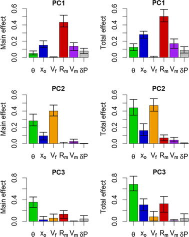

  

  Main (left) and Total (right) effects for the difference cyclone characteristics regarding the occurrence of the pattern described by the three first PCs. The error bars are derived from the 5 and 95 % quantiles of the bootstrap procedure

• The second PC₂ can be seen as the occurrence of a regime shift at s = 0: input parameters resulting in positive (resp. negative) expansion weights (dashed and dotted lines in Fig. 12b) lead to a switch from a first regime for s < 0 where H _S is above (resp. below) the mean function and to a second one for s > 0 where H _S is below (resp. above) the mean function: this mode of variation can be interpreted as an inversion of the rate of H _S evolution before and after landfall;

• The third PC₃ (Fig. 12c) can be interpreted as the occurrence of two regime shifts in the landfall region (approximately between s ~ −90 km and s ~ 20 km) corresponding to the peak of wave heights. Input parameters resulting in positive expansion weights lead to a switch from a first regime where H _S is above the mean function before and after the landfall region to a second one where H _S suddenly drops in the landfall region, which results in the occurrence of two peaks of wave height: this mode of variation expresses a very particular situation when the eye of the cyclone crosses Sainte-Suzanne.

The sensitivity measures for each of these modes are provided in Fig. 12. To support the discussion and to get a more physical picture of the influences of the cyclone parameters, Fig. 13 (top) provides three examples for each PC: scenarios n°64–84 show a high contribution of PC₁ while scenario n°18–51 and n°74–32 reveal substantial contribution of, respectively, PC₂ and PC₃. The spatial fields of the corresponding H _S at relevant time steps are also provided to support the discussion.

Fig. 13

Scenarios illustrating the pattern induced by PC₁ (a), PC₂ (b) and PC₃ (c). On the maps, the colours represent the significant wave height and the white contours, the wave peak period (relevant time steps were selected to illustrate the text). The red circle indicates the distance of 100 km away from the centre of Reunion Island and the white line gives the cyclone track in the vicinity of Reunion Island

Let us first consider PC₁. Figure 12 (top) indicates that the maximum cyclone radius R _m has the largest influence regarding this response (with main effect >40 %). The second most important parameters are the relative landfall position x _o with a high interaction term (total effect exceeds by ~10 % the main effect) and the maximum wind speed V _m with contributions of ~15 % (but a little interaction term). The forward speed V _f appears to be a negligible contributor to uncertainty (Fig. 12, top right). Scenario n°64 (Fig. 13a) provides a good example of the high influence of R _m and V _m. This scenario exhibits large radius (~40 km) and maximum wind speed (~125 kt), that both increase the wave heights. Besides, the relative landfall position and angle of approach make the core of the wave field pass very close to Sainte-Suzanne so that the peak of wave height is amplified (Fig. 13a). These characteristics result in overall high H _S values at Sainte-Suzanne all along the cyclone track. On the contrary, scenario n° 84 has a moderate wind speed (~90 kt) and a very small radius (~15 km) associated with a relative landfall position on the other side of the island that induce overall low H _S values at Sainte-Suzanne. These physical behaviours were also verified on other members of the simulation scenarios.

Considering PC₂, the largest contributor is the forward speed V _f (Fig. 12, middle) with an influence of almost 50 %. The second most important parameter is the angle of approach θ with a high interaction term (total effect exceeds by ~15 % the main effects) with a contribution of ~30 %. To illustrate and clarify this, let us first consider scenario n° 51, which exhibits a high forward speed of ~18 kt (Fig. 13b). If the fast cyclone motion tends to increase the height of waves in the left-forward quadrant, it also limits the forward propagation of waves ahead the eye so that they lag near and behind the eye (as explained in Sects. 2.3, 4.2). This results in low early wave heights at Sainte-Suzanne followed by (1) a large and abrupt rise occurring within a short period before landfall and (2) a slower decrease of wave heights after landfall. If we now pay attention to scenario n° 18 (with a low forward speed around 10 kt, Fig. 13b), we see that the shape of the wave pattern and the associated H _S series at Sainte-Suzanne have opposite behaviours than those of scenario n°51. Finally, the angle of approach together with the landfall position influence the relative position of Sainte-Suzanne to both the main propagation direction and the core of the wave field. This modulates the effect of the translation speed on H _S evolution and then the influence regarding PC₂.

Finally, the analysis for PC₃ highlights the high individual contribution of θ (main effect of ~40 %) and the high contribution of x _o and R _m regarding interactions with high total effects of the order of ~30 % (Fig. 12, bottom, right). This can be explained by the important roles that play these three parameters in the size and relative position of the eye to the studied site so that variations in their combination may change the form and the way the wave pattern crosses the site. For example, in scenario n°32 (Fig. 13c), the radius of the cyclone is quite large (~45 km), so that Sainte-Suzanne is affected successively by the circular wave pattern generated in two opposite quadrants of the cyclone separated by a calmer zone, which creates the “double peak” in the H _S series. As for the scenario n° 74 (Fig. 13c), the radius of maximum wind is too small (~10 km) to obtain a distinct circular structure of the wave field. This results in a single peak when the eye of the cyclone crosses the site.

4.5 Summary

Using the results of the multi-mode dynamic sensitivity analysis, the identification of the most important cyclone characteristics can be performed depending on the objective of the study.

• If the interest is on the identification of the most important parameter whatever s, the aggregated option should be selected. Here, its application highlights the large contribution of the radius of maximum wind R _m as well as the moderate role of the landfall position x _o;

• If the interest is on the phasing of the influence and the understanding of the role of the different parameters given the cyclone positions, the step-by-step option should be selected. Here it reveals (1) a major influence of V _f when the cyclone is still far away from the site (2) the high contribution of R _m in the vicinity of the studied site except when the cyclone is the closest to the island at s = 0 where the landfall position (here x _o) is the most important characteristic that determines the amplitude of peak of wave heights;

• Finally, the mode-based option should be viewed as a supplement of the two first options: the role of the cyclone characteristics regarding specific evolution patterns can be investigated. In our case, the forward speed V _f, though of low-to-moderate importance (when the cyclone approaches the site) considering the step-by-step and the aggregated option, appears to play a major role for the initiation of a turning point (regime shift) at s = 0 meaning that depending on this characteristic, the H _S values may be categorised as moderate for s < 0, but when the cyclone hits the Reunion Island for s = 0, the regime might switch to high H _S values.

Table 2 summarises the main conclusions of the multi-look dynamic sensitivity approach.

Table 2 Synthesis of the importance ranking: ++ high influence (largest main effect), +/− moderate (main effect between 10–20 %); − low-to-moderate (main effect below 10 %), – negligible (total effect close to 0). The relative cyclone position s is expressed in km

5 Concluding remarks and further works

The problem of dynamic sensitivity analysis can be looked in different ways. In the present study, we proposed a whole strategy for getting a deep insight in the role played by the different cyclone characteristics regarding the variability of H _S as a function of the relative cyclone position s: this was done by adopting three perspectives to this dynamic VBSA. A particular attention was paid to relate those conclusions with physical interpretations; though some of them were very intuitive, the proposed strategy has the great benefit to quantify the different contributions given the assumptions on their variations.

These conclusions are valid keeping in mind that we considered a restricted sample of cyclones all passing close to Reunion Island and that we assumed that the cyclone characteristics are held constant over time. We acknowledge that this last point remains a simplification, and accounting for more complex and time-varying characteristics (for example by using statistical-based datasets such as the one constituted by Emanuel et al. (2006)) constitutes a line for future research. From a methodological point of view, this imposes to consider functional variables for both inputs and outputs of the meta-model-based procedure, i.e. to perform function-on-function high-dimensional regression, which still constitute a matter of ongoing research due to the so-called “small n, large p” paradigm (e.g. Morris 2015). Second, we focused on H _S series which are the primary quantities of interest for local flooding risk assessment. Yet, a second necessary step should focus on the joint analysis of the series for both wave period and direction, which should also play a major role in wave overtopping potential.

Finally, it should be underlined that the meta-models were used here for computing variance-based sensitivity measures so that the meta-model error (of low level as indicated by the results of the cross-validation procedure) has little influence on the importance ranking (as indicated by the bootstrap analysis). Yet, such meta-models could also be used to perform predictions (forecasting), for instance for early-warning purposes or for assessing low probability/high consequences events. Although, this particular application is expected to require (1) the consideration of a complete data set including more distant and various tracks as well as time-varying cyclone characteristics as mentioned above (2) more robust functional meta-models whose accuracy and predictive quality should be more carefully accounted for (for instance by relying on existing studies for scalar variables, Janon et al. 2014).

Appendices

Appendix 1: generalisation of Sobol’ indices for multivariate (functional) outputs

Consider the functional output H _S(s) discretised on a regular grid of track positions s viewed as vectors of large but finite dimension, and X the vector of input parameters following Gamboa et al. (2014), the generalised Sobol’ index S _agg,i for the ith parameter holds as:

$$S_{agg,i} = \frac{{Tr({\mathbf{C}}_{i} )}}{{Tr({\mathbf{C}})}}$$

(6)

where Tr is the trace; ${\mathbf{C}} = \text{cov} \left( {{\mathbf{H}}_{S} } \right)$ and ${\mathbf{C}}_{i} = \text{cov} \left( {E\left( {\left. {{\mathbf{H}}_{S} } \right|X_{i} } \right)} \right)$ are covariance matrices.

Equation 6 is the index of first order, which measures the relative contribution of the ith input parameter. Higher order indices as well as total effect can also be defined in the same way than the Sobol’ indices for scalar output. These sensitivity measures can be estimated using a pick-and-freeze as proposed by Gamboa et al. (2014).

Appendix 2: correlation function adapted to categorical inputs

This appendix is mainly based on Storlie et al. (2013): Sect. 2.1. A variety of correlation (and covariance) functions have been proposed in the literature (see e.g. Stein 1999). The commonly used model is the exponential correlation function defined as follows:

$$R({\text{u}};{\text{v}}) = \exp \left( - \sum\limits_{i = 1}^{d} {\frac{{\left| {u_{i} - v_{i} } \right|^{{\rho_{i} }} }}{{\beta_{i} }}}\right)$$

(7)

where ρ is the vector of power parameters (typically between 0 and 2) controlling the shape of the correlation function, and the vector β determines the rate at which the correlation decreases as one moves in the ith direction (with i from 1 to d). Intuitively, if u = v then the correlation is 1, whereas if the distance between both vectors tends to the infinity, then the correlation tends to 0. In this article, the difficulty is to handle continuous and categorical input variables (in our case, these correspond to the limited number of scenarios of cyclone tracks θ): to do so, we chose to a covariance function, which is adapted to this case, as described by Storlie et al. (2013). Consider x ₁,…, x _q the continuous input parameters, x _q+1,…, x _d the unordered categorical ones. Consider first the case of one categorical variable x _j, a possible correlation function is:

$$R({\text{x}}_{j} ;x_{j}^{*} ) = \exp \left( { - \frac{{Ind\left( {x_{j} \ne x_{j}^{*} } \right)}}{\beta }} \right)$$

(8)

where Ind is the indicator function so that Ind = 1 if ${\text{x}}_{j} \neq x_{j}^{*}$ and 0 otherwise; β is the corresponding length-scale parameter.

By using Eq. 7 for continuous variables, a separable correlation function (i.e. product of one-dimensional correlation) can be defined:

$$R({\text{x}}_{j} ;x_{j}^{*} ) = \exp \left( - \sum\limits_{i = 1}^{q} {\frac{{\left| {x_{i} - x_{i}^{*} } \right|^{{\rho_{i} }} }}{{\beta_{i} }} - \sum\limits_{i = q + 1}^{d} {\frac{{Ind\left( {x_{j} \ne x_{j}^{*} } \right)}}{{\beta_{i} }}} }\right)$$

(9)

As underlined by Storlie et al. (2013), the correlation as aforedescribed is isotropic, which is a reasonable assumption in many cases. More sophisticated approaches may rely on Qian et al. (2008).

Appendix 3: Principal Component Analysis

The PCA decomposition is based on the empirical eigenfunctions and vectors of the variance-covariance matrix ${\varvec{\Sigma}} = {}^{t}{\mathbf{H}}_{S}^{C} \cdot {\mathbf{H}}_{S}^{C}$ with ${\mathbf{H}}_{S}^{C}$ the matrix of n ₀ N-dimensional H _S series centred around the mean function ${\bar{\text{H}}}_{S}^{{}}$. Let us define the eigenvalues $\lambda_{1} > \lambda_{2} > \cdots > \lambda_{N}$ of ${\varvec{\Sigma}}$ ordered in increasing order and V a N×N matrix of normalised eigenvectors v of ${\varvec{\Sigma}}$, each column being associated with a given eigenvalue λ. The n ₀×N matrix ${\mathbf{H}}^{PC}$ of principal components PCs holds as follows:

$${\mathbf{H}}^{PC} = {\mathbf{H}}_{S}^{C} \cdot{\mathbf{V}}$$

(10)

The column h of ${\mathbf{H}}^{PC}$ are mutually orthogonal linear combination of the columns of ${\mathbf{H}}_{S}^{C}$ so that ${\mathbf{h}}_{k} = {\mathbf{H}}_{S}^{C} \cdot{\mathbf{v}}_{k}$ and $\left\| {{\mathbf{h}}_{k} } \right\|^{2} = \lambda_{k}$. By construction the trace of ${\mathbf{H}}^{PC}$ is the same as Σ so that the d first PCs concentrate a given level of explained variance, aka inertia, i.e. of a given amount of information.

References

Amante C, Eakins BW (2009) ETOPO1 1 arc-minute global relief model: procedures, data sources and analysis. NOAA Technical Memorandum NESDIS NGDC-24, March 2009
Antoniadis A, Helbert C, Prieur C, Viry L (2012) Spatio-temporal metamodeling for West African monsoon. Environmetrics 23(1):24–36
Archer GEB, Saltelli A, Sobol’ IM (1997) Sensitivity measures, ANOVA-like techniques and the use of bootstrap. J Stat Comput Simul 58(2):99–120
Ardhuin F, Rogers WE, Babanin AV, Filipot J, Magne R, Roland A, van der Westhuysen A, Queffeulou P, Lefevre J, Aouf L, Collard F (2010) Semiempirical dissipation source functions for ocean waves. Part I: definition, calibration, and validation. J Phys Oceanogr 40(1):1917–1941
Campbell K, McKay MD, Williams BJ (2006) Sensitivity analysis when model outputs are functions. Reliab Eng Syst Safety 91:1468–1472. doi:10.1016/j.ress.2005.11.049
Cazes-Duvat V, Paskoff R (2004) Les littoraux des Mascareignes entre nature et aménagement, L’Harmattan (in French)
Chateauminois E, Thirard G, Pedreros R, Longueville F (2014) Caractérisation et cartographie des aléas côtiers pour l’élaboration du Plan de Prévention des Risques Littoraux des communes du Nord-Est de la Réunion. BRGM technical report BRGM/RP-64088-FR (in French)
Diamond HJ, Lorrey AM, Knapp KR, Levinson DH (2012) Development of an enhanced tropical cyclone tracks database for the Southwest Pacific from 1840 to 2010. Int J Climatol 32(14):2240–2250
Emanuel K, Ravela S, Vivant E, Risi C (2006) A statistical deterministic approach to hurricane risk assessment. Bull Am Meteorol Soc 87(3):299–314
Forrester AIJ, Sobester A, Keane AJ (2008) Engineering design via surrogate modelling: a practical guide. Wiley, Chichester
Gamboa F, Janon A, Klein T, Lagnoux A (2014) Sensitivity analysis for multidimensional and functional outputs. Electron J Stat 8(1):575–603
Hastie T, Tibshirani R, Friedman J (2009) The elements of statistical learning: data mining, inference, and prediction, 2nd edn. Springer, New York
Holland GJ (1980) An analytic model of the wind and pressure profiles in hurricanes. Mon Weather Rev 108(8):1212–1218
Iooss B, Lemaître P (2015) A review on global sensitivity analysis methods. In: Meloni C, Dellino G (eds) Uncertainty management in simulation-optimization of complex systems: algorithms and applications. Springer, New York, pp 101–122
Irish JL, Song YK, Chang K-A (2011) Probabilistic hurricane surge forecasting using parameterized surge response functions. Geophys Res Lett 38(3):L03606
Janon A, Nodet M, Prieur C (2014) Uncertainties assessment in global sensitivity indices estimation from metamodels. Int J Uncertain Quantif 4(1):21–36
Jansen MJW (1999) Analysis of variance designs for model output. Comput Phys Commun 117:35–43
Jia G, Taflanidis AA (2013) Kriging metamodeling for approximation of high-dimensional wave and surge responses in real-time storm/hurricane risk assessment. Comput Methods Appl Mech Eng 261:24–38
Jia G, Taflanidis AA, Norterto N-C, Melby J, Kennedy A, Smith J (2015) Surrogate modeling for peak and time dependent storm surge prediction over an extended coastal region using an existing database of synthetic storms. Nat Hazards. doi:10.1007/s11069-015-2111-1
Jolliffe I (2002) Principal component analysis. Wiley, New York
Jumeaux G, Quetelard H, Roy D (2011) Atlas Climatique de La Réunion of Météo-France, Météo-France technical report (in French)
Kennedy AB, Westerink JJ, Smith J, Taflanidis AA, Hope M, Hartman M, Tanaka S, Westerink H, Cheung KF, Smith T, Hamman M, Minamide M, Ota A (2012) Tropical cyclone inundation potential on the Hawaiian islands of Oahu and Kauai. Ocean Model 52–53:54–68
Kleijnen JP (2014) Simulation-optimization via Kriging and bootstrapping: a survey. J Simul 8(4):241–250
Le Cozannet G, Rohmer J, Cazenave A, Idier D, van De Wal R, De Winter R, Oliveros C (2015) Evaluating uncertainties of future marine flooding occurrence as sea-level rises. Environ Model Softw 73:44–56
Lecacheux S, Pedreros R, Le Cozannet G, Thiébot J, De La Torre Y, Bulteau T (2012) A method to characterize the different extreme waves for islands exposed to various wave regimes: a case study devoted to Reunion Island. Nat Hazards Earth Syst Sci 12:2425–2437. doi:10.5194/nhess-12-2425-2012
Liu H, Xie L, Pietrafesa LJ, Bao S (2007) Sensitivity of wind waves to hurricane wind characteristics. Ocean Model 18(1):37–52. doi:10.1016/j.ocemod.2007.03.004
McKay MD, Beckman RJ, Conover WJ (1979) A comparison of three methods for selecting values of input variables in the analysis of output from a computer code. Technometrics 21:239–245
Morris JS (2015) Functional regression. Ann Rev Stat Appl 2(1):321–359
Niedoroda AW, Resio DT, Toro G, Divoky D, Reed C (2008) Efficient strategies for the joint probability evaluation of storm surge hazards. In: Proceedings of solutions to coastal disasters congress, ASCE, Reston, VA, pp 242–255
Niedoroda AW, Resio DT, Toro G, Divoky D, Reed C (2010) Analysis of the coastal Mississippi storm surge hazard. Ocean Eng 37:82–90
Osuri KK, Mohanty UC, Routray A, Mohapatra M (2012) The impact of satellite-derived wind data assimilation on track, intensity and structure of tropical cyclones over the North Indian Ocean. Int J Remote Sens 33(5):1627–1652
Phadke AC, Martino CD, Cheung KF, Houston SH (2003) Modeling of tropical cyclone winds and waves for emergency management. Ocean Eng 30(4):553–578
Qian P, Wu H, Wu CFJ (2008) Gaussian process models for computer experiments with qualitative and quantitative factors. Technometrics 50:383–396
R Development Core Team R (2014) A language and environment for statistical computing. R Foundation for Statistical Computing, Vienna, Austria, (2014). ISBN 3-900051-07-0. http://www.R-project.org/
Ramsay JO, Silverman BW (2005) Functional data analysis. Springer, New York
Resio D, Irish J, Cialone M (2009) A surge response function approach to coastal hazard assessment. 1: basic concepts. Nat Hazards 51(1):163–182
Rohmer J (2014) Dynamic sensitivity analysis of long-running landslide models through basis set expansion and meta-modelling. Nat Hazards 73(1):5–22
Rohmer J, Foerster E (2011) Global sensitivity analysis of large scale landslide numerical models based on the Gaussian Process meta-modelling. Comput Geosci 37:917–927
Rousseau M, Cerdan O, Ern A, Le Maître O, Sochala P (2012) Study of overland flow with uncertain infiltration using stochastic tools. Adv Water Resour 38:1–12. doi:10.1016/j.advwatres.2011.12.004
Sacks J, Welch WJ, Mitchell TJ, Wynn HP (1989) Design and analysis of computer experiments. Stat Sci 4:409–435
Saltelli A, Annoni P (2010) How to avoid a perfunctory sensitivity analysis. Environ Model Softw 25:1508–1517
Saltelli A, Ratto M, Andres T, Campolongo F, Cariboni J, Gatelli D, Saisana M, Tarantola S (2008) Global sensitivity analysis: The Primer. Wiley, Chichester 304 pp
Saltelli A, Annoni P, Azzini I, Campolongo F, Ratto M, Tarantola S (2010) Variance based sensitivity analysis of model output. Design and estimator for the total sensitivity index. Comput Phys Commun 181:259–270
Shapiro L (1983) The asymmetric boundary layer flow under a translating hurricane. J Atmos Sci 40:1984–1998
Song YK, Irish JL, Udoh IE (2012) Regional attributes of hurricane surge response functions for hazard assessment. Nat Hazards 64(2):1475–1490
Stein ML (1999) Interpolation of spatial data: some theory for kriging. Springer, New York
Storlie CB, Swiler LP, Helton JC, Sallaberry CJ (2009) Implementation and evaluation of nonparametric regression procedures for sensitivity analysis of computationally demanding models. Reliab Eng Syst Saf 94:1735–1763
Storlie CB, Reich BJ, Helton JC, Swiler LP, Sallaberry CJ (2013) Analysis of computationally demanding models with continuous and categorical inputs. Reliab Eng Syst Saf 113:30–41
Terry JP, Gienko G (2010) Climatological aspects of South Pacific tropical cyclones, based on analysis of the RSMC-Nadi (Fiji) regional archive. Clim Res 42(3):223–233
Tolman HL (2014) User manual and system documentation of WAVEWATCH-III version 4.18. NOAA/NWS/NCEP/MMABTech
Wang Y, Holland GJ (1996) Tropical cyclone motion and evolution in vertical shear. J Atmos Sci 53:3313–3332
Xie L, Bao S, Pietrafesa LJ, Foley K, Fuentes M (2006) A real-time hurricane surface wind forecasting model: formulation and verification. Mon Weather Rev 134:1355–1370
Acknowledgments
This work is supported by the French National Research Agency within the SPICy project (ANR – 14 – CE03 – 0013). More details on the project are available at http://spicy.brgm.fr. The authors thank the Region of La Reunion for providing the wave measurements deployed and analysed by NortekMed in front of the coastal road at station RN4. We also acknowledge the PREVIMER team, and more specifically F. Ardhuin (LOPS), for making available the unstructured grid (Reunion-UG) used for wave modelling at rank 2 (see http://www.previmer.org/).
Author information
Authors and Affiliations
Corresponding author