
Abstract
Although the boundedly rational (BR) day-to-day dynamic proposed in Guo and Liu (Transp Res B 45(10):1606–1618, 2011) managed to model drivers’ transient behaviour under disequilibrium in response to a network change, its stability property remains unanswered. To better understand the boundedly rational (BR) dynamic, this paper initiates the stability analysis of the BR dynamic. As we will show, the BR dynamic is a piecewise affine linear system consisting of multiple subsystems. The conventional Lyapunov theorem commonly used in the literature cannot be applied and thus a multiple Lyapunov method is adopted. The multiple Lyapunov method requires that the Lyapunov values decrease when trajectories evolve as time elapses and the decreasing rate is bounded above. We can show that within each subsystem, the Lyapunov function decreases at an exponential rate. Meanwhile, when trajectories reach boundaries between subsystems, they can either slide or switch and the Lyapunov value also changes across subsystems at a negative rate. Therefore, the BR dynamic is stable. A small network example is given to illustrate this method.
1 Introduction
The deterministic day-to-day traffic dynamic is to model drivers’ transient behaviour under disequilibrium assuming drivers follow the Wardrop’s first principle. There is a large body of literature on deterministic dynamical systems: the proportional-switch adjustment process (Smith 1979), the tatonnement dynamic (Friesz et al. 1994), the projected dynamical system (Nagurney and Zhang 1997) and the link-based day-to-day dynamic (He et al. 2010). All these dynamics are proven to stabilize at the user equilibrium (UE) after a long enough time period.
Though the aforementioned dynamical systems can capture the system’s evolving process towards the equilibrium, they are unable to interpret the traffic pattern change across the I-35W Bridge in Minnesota before its collapse and after its reopening. It was observed that under a similar demand level and the almost identical network topology, the daily traffic across the restored bridge decreased by 20,000 vehicles on average compared to that on the old one. The perfectly rational day-to-day dynamics are incapable of capturing this phenomenon, because the dynamics before the bridge’s collapse and after its reopening would evolve to the same user equilibrium solution given the same monotonically increasing link performance functions. Thus the traffic flow across the bridge should not change. Guo and Liu (2011) proposed a boundedly rational (BR) day-to-day dynamic, whose fixed point is defined as “boundedly rational user equilibria” (BRUE). Generally the BRUE is not unique and all equilibria forms a BRUE flow set. The BR dynamic can successfully explain the above phenomenon, because the flow pattern driven by the BR dynamic will evolve from one fixed point (before its collapse) towards another one (after its reopening) within the BRUE solution set, resulting in two different equilibrium states.
As opposed to ‘rationality as optimization’, Herbert Simon proposed that people are boundedly rational in their decision-making processes (Simon 1955). Mahmassani and Chang (1987) first proposed that travellers are boundedly rational in making departure time choices at a single bottleneck. A number of models also incorporated BR to people’s travel decision-making processes (Hu and Mahmassani 1997; Mahmassani and Liu 1999; Szeto and Lo 2006; Lou et al. 2010; Guo and Liu 2011). In particular, Lou et al. (2010) and Di et al. (2013) gave the mathematical formulation of boundedly rational user equilibrium on route choice and Guo and Liu (2011) was the first one to incorporate BR into the day-to-day dynamic.
Although the BR day-to-day dynamic has the flexibility to model drivers’ transient behaviour, its stability property remains unanswered. In reality, the transportation network is exposed to various temporary changes, such as construction, lane closure or even some unexpected disruption. The stability analysis addresses whether a small perturbation to a road system resting at an equilibrium state will make the system to stabilize to the same equilibrium or diverge to an unstable state, after a planned change or an unexpected event occurs (Watling and Cantarella 2013). Moreover, the stability represents the ‘attainability’ of an equilibrium. If the system is not stable, the equilibrium is unattainable and it is impossible to propose any network design strategies to support transportation supply design (Cantarella et al. 2010; Watling and Cantarella 2013). In summary, the stability is a crucial feature of the dynamical system. To better understand the characteristic of the BR dynamic, its stability property needs to be explored. Depending on the number of equilibria a dynamical system contains, the methodologies of the stability analysis are different.
When there exists one equilibirum, the stability of deterministic dynamics usually can be proved by defining a distance measure as the Lyapunov function: proportional-switch adjustment process (Smith 1979) utilized the difference between path costs; while the tatonnement dynamic (Friesz et al. 1994), the projected dynamical system (Nagurney and Zhang 1997) and the link-based day-to-day dynamic (Han and Du 2012; He 2010) used the distance between the current flow pattern and the equilibrium. The dynamical system is stable when the Lyapunov function monotonically reduces to zero.
Watling (1999) raised the issue of the stability of the stochastic day-to-day dynamic with multiple equilbira. Watling and Hazelton (2003) characterized the stability as ‘attractiveness’ of an equilibrium solution given a perturbation to the flow levels, and this attractiveness was governed by certain driver behavior rules. Among multiple user equilibria, some are ‘user-optimal’ while others are not, then the stable ones in the sense of user-optimal should be the main focus. Cantarella et al. (2013) proposed a nonlinear deterministic dynamic modeling two mode choices (bus v.s. car). It contains multiple equilibria and one equilibrium is stable if its Jacobian matrix has modulus of less than one.
The stability of the BR dynamic reveals whether flow patterns at one BRUE will return to another BRUE given a perturbation to the network. This paper will propose a methodology to prove the stability of the BR dynamic. The rest of the paper is organized as follows. After giving a brief description of the BR dynamic in Section 2, we then reformulate it as a piecewise affine (PWA) linear system composed of multiple subsystems in Section 3. The stability is analyzed for the subsystems of the BR dynamic in Section 4 and for boundaries separating subsystems in Section 5. To prove the stability of the dynamic across boundaries separating subsystems, two trajectory patterns: sliding and switching are studied. The stability is illustrated by an example in Section 6. Finally, conclusions and future research directions are discussed in Section 7.
2 Introduction to the Boundedly Rational Dynamic
The traffic network is represented by a directed graph that includes a set of consecutively numbered nodes, 𝓝, and a set of consecutively numbered links, ℒ. Let 𝒲 denote the O-D pair set and w ∈ 𝒲 is connected by a set of simple paths (composed of a sequence of distinct nodes), 𝓟w, through the network. The traffic demand between each OD pair is d w. Let \({f^{w}_{i}}\) denote the flow on path i ∈ 𝓟w for OD pair w, then the path flow vector is \(\mathbf {f}=\{\mathbf {f}^{w}\}^{w \in \mathcal { W}}=\{{f^{w}_{i}}\}_{i \in \mathcal {P}^{w}}^{w \in \mathcal {W}}\). The feasible path flow set is to assign the traffic demand on the feasible paths: \(\mathcal {F} \triangleq \{\mathbf {f}: \mathbf {f} \geqslant \mathbf {0}, \sum \limits _{i \in \mathcal {P}^{w}} {f_{i}^{w}}=d^{w}, \forall w \in \mathcal {W} \}\). Denote x a as the link flow on link a, then the link flow vector is \(\mathbf {x}=\{x_{a}\}_{a \in \mathcal {X}}\). Each link a ∈ ℒ is assigned a cost function which is a function of the link flows, written as c(x). Let \(\delta _{a,i}^{w}=1\) if link a is on path i connecting OD pair w, and 0 if not; then \(\Delta \triangleq \{ \delta _{a,i}^{w} \}_{a \in \mathcal {L}, i \in \mathcal {P}}^{w \in \mathcal {W}}\), denotes the link-path incidence matrix. Therefore \({f^{w}_{i}}=\sum \limits _{a} \delta _{a,i}^{w} x_{a}\), and it can be rewritten in a vector form as x = Δ f. Denote \({C^{w}_{i}}(\mathbf {f})\) as the path cost on path i for OD pair w, then the path cost vector \(C(\mathbf {f})\triangleq \{{C^{w}_{i}}(\mathbf {f})\}_{i \in \mathcal {P}}^{w \in \mathcal {W}}\). So C(f) = Δ T c(x) under the additive path cost assumption.
In this paper, we make three assumptions:
-
the link cost is separable, i.e., c i (x) = c i (x i ),i = 1, ⋯ ,n, where n is the total number of links in the network;
-
the link cost is affine linear and strictly monotone, i.e., c(x) = H x + a, where H = {h ij (x)},i,j = 1, ⋯ ,n and H is a positive-definite diagonal matrix;
-
the network contains one OD pair connecting n links in parallel. Therefore the “link” and the “path” are the same and are interchangeable in the following.
The continuous-time boundedly rational dynamic proposed in Guo and Liu (2011) can be written in the form of differential algebraic equation (ADE):
where, \(\mathbf {x} \triangleq \{ x_{a} \}_{a \in \mathcal {L}}\): the flow vector;
\(\dot {\mathbf {x}}\): the link flow change w.r.t. time;
u: the target link flow pattern;
β: a positive constant determining the flow changing rate, 0 < β < 1;
\(\mathcal {X}^{br}(c(\mathbf {x}))\): the acceptable link flow pattern induced by x, which will be discussed in the following; \(\text {Pr}_{\mathcal {X}^{br}(c(\mathbf {x}))}(\mathbf {x})\): a projection operator, projecting x onto the set \(\mathcal {X}^{br}(c(\mathbf {x}))\).
If we discretize this dynamic with respect to time, then the discrete-time version is a day-to-day flow adjusting process. It can be explained as (Guo and Liu 2011): on each day, the flow pattern tends to move from the current pattern x towards the target pattern u, based on the current day’s link cost c(x).
2.1 Formulating the Acceptable Sets
The acceptable set induced by the link cost c(x) is defined as:
After the acceptable set \(\mathcal {P}^{br} (c(\mathbf {x}))\) is known, we assign the demand to those acceptable links. Then the acceptable link flow pattern, denoted by \(\mathcal {X}^{br}(c(\mathbf {x}))\), can be mathematically expressed as:
where, v is a n × 1 vector with \(v_{i}= \begin {cases} 1, \mbox { if } c_{i}(\mathbf {x})\leqslant \displaystyle \min _{j \in \mathcal {A}} c_{j}(\mathbf {x})+\varepsilon \\ 0, \mbox { o.w.} \end {cases}\).
Assume the acceptable set contains the first p paths, while the unacceptable set has the rest n − p paths, i.e., the acceptable set a = {1, ⋯ ,p} and the unacceptable set u = {p + 1, ⋯ ,n}. Rearrange the elements in v, such that the first p elements are ones and the rest are zeros, we can rewrite v as: \(\mathbf {v}=\begin {pmatrix} \mathbf {1}_{a}\\ \mathbf {0}_{u} \end {pmatrix}\), where 1 a is a p × 1 vector with all elements equal to one, and 0 u is a (n − p)×1 vector with all elements equal to zero. No flow is assigned to n − p unacceptable paths, i.e., x u =0 (n − p)×1. An acceptable path flow pattern x can be also divided into two parts: \(\mathbf {x}=\begin {pmatrix} \mathbf {x}_{a}\\ \mathbf {0}_{u} \end {pmatrix}\). Then Eq. 2.3 can be rewritten as:
Guo and Liu (2011) pointed out that the fixed points of the BR dynamic is the “boundedly rational user equilibria (BRUE)”, which is defined as (Di et al. 2013; Guo and Liu 2011):
Definition 2.1
For a given ε ⩾ 0, a feasible flow vector x ∈ 𝒳 is said to be a boundedly rational user equilibrium (BRUE) path flow pattern, denoted by x BRUE , if
where ε is the indifference band, indicating the rationality level of drivers’ behavior. In this study, we assume ε is a known parameter.
All the flow patterns satisfying Definition (2.5) constitute a set, called the BRUE flow solution set:
2.2 Solving the Target Flow Projection
The BR dynamic defined in Eq. 2.1 is composed of two equations: the ordinary differential equation (2.1a), and the relationship between x and u defined in Eq. 2.1b. To better study this dynamic, we need to solve the target flow u first.
Equation 2.1b indicates that, u is the projection point of x onto the acceptable link flow set \(\mathcal {X}^{br}(c(\mathbf {x}))\). Therefore u can be computed by solving the projection from the geometrical point of view. Recall that x is composed of two parts: x a and x u . Consequently u can be decomposed into two parts: \(\mathbf {u}=\left (\begin {array}{c}\mathbf {u}_{a}\\ \mathbf {0}_{u}\end {array}\right ),\) and we only need to derive the formulation for u a .
Let the point M represent the current flow x a , and the hyperplane P be the acceptable path flow set \(\mathcal {X}^{br}(c(\mathbf {x}))\) in the form of Eq. 2.4. To find a mathematical formulation of \(\text {Pr}_{\mathcal {X}^{br}(c(\mathbf {x}))}(\mathbf {x})\) is equivalent to finding a projection point U : u a , of a given point M : x a to a hyperplane P (See Fig. 1).

Illustration of the projection
By solving the following minimization program:
We obtain the projection u as:
When the current link flow pattern varies, it has a different target flow. So u is a function of x.
3 Discontinuous BR Dynamic
3.1 BR Dynamic within Subsystems
Given the acceptable set a = {1, ⋯ ,p} and the unacceptable set u = {p + 1, ⋯ ,n}, substitute the specific form of u into Eq. 2.1a. Then the BR dynamic can be reduced as:
Dynamic (3.1) tells us, if link i is unacceptable, its flow keeps decreasing. Due to flow conservation, the total reduced flows from unacceptable links will be evenly distributed to p acceptable ones. Mathematically speaking,
-
if \(c_{i}(\mathbf {x}) > \displaystyle \min _{j \in \mathcal {A}} c_{j}(\mathbf {x})+\varepsilon \): according to Definition (2.2), i is unacceptable and j is acceptable. Then \(\dot {x}_{i}<0,\dot {x}_{j}>0\). Mathematically,
$$ c_{i}(\mathbf{x}) > \displaystyle\min\limits_{j \in \mathcal{A}} c_{j}(\mathbf{x})+\varepsilon\Rightarrow \dot{x}_{i}<0, \dot{x}_{j}>0;$$(3.2) -
if \(c_{i}(\mathbf {x}) < \displaystyle \min\limits _{j \in \mathcal {A}} c_{j}(\mathbf {x})+\varepsilon \): both i and j are acceptable, then \(\dot {x}_{i}=\dot {x}_{j}>0\). Mathematically,
$$ c_{i}(\mathbf{x}) < \displaystyle\min\limits_{j \in \mathcal{A}} c_{j}(\mathbf{x})+\varepsilon\Rightarrow \dot{x}_{i}=\dot{x}_{j}>0.$$(3.3)
Remark
This dynamic property is only valid for the network with one OD pair connecting parallel links.
When the acceptable set is not given, we need to enumerate all possible acceptable sets. In a network with n links, there are 2n − 1 possible acceptable sets. Because any link can be acceptable or unacceptable and at least one link needs to be acceptable.
Dynamic (3.1) behaves differently when the current flow pattern is within a different region. Then the BR dynamic can be extended to a more general matrix form from Eq. 3.1:
where,
x: the state;
A q (x),b q (x): the coefficient matrix and vector in subsystem q;
n: the dimension of the state;
q: the q th subsystem index.
Here \(A_{q}(\mathbf {x}) = \beta \begin {bmatrix} -\frac {\mathbf {1}_{p}\mathbf {1}_{p}^{T}}{\mathbf {1}_{p}^{T}\mathbf {1}_{p}} & \mathbf {0}^{T}_{(n-p)\times p}\\ \mathbf {0}_{(n-p)\times p} & -\mathbf {I}_{n-p} \end {bmatrix}\), \(b_{q}(\mathbf {x}) = \beta \begin {pmatrix} \frac {d\mathbf {1}_{p}}{\mathbf {1}_{p}^{T}\mathbf {1}_{p}}\\ \mathbf {0}_{(n-p)\times 1} \end {pmatrix}\), where I n − p is a (n − p)×(n − p) identity matrix. The reason why A and b are dependent on the state variable x is that, for a different flow pattern, the acceptable path set is different. The coefficient matrix A has two blocks on the diagonal and the zero off-diagonal matrices. Let \(\mathbf {A}_{p}=-\beta \frac {\mathbf {1}_{p}\mathbf {1}_{p}^{T}}{\mathbf {1}_{p}^{T}\mathbf {1}_{p}} =\begin {bmatrix} -\frac {\beta }{p} & \cdots & -\frac {\beta }{p} \\ & \ddots &\\ -\frac {\beta }{p} & \cdots & -\frac {\beta }{p} \end {bmatrix}\), A n − p =−β I n − p , \(\mathbf {b}_{p}=\beta \frac {d\mathbf {1}_{p}}{\mathbf {1}_{p}^{T}\mathbf {1}_{p}}\), b n − p =0 (n − p)×p . Then
3.2 Piecewise Affine Linear System
The hybrid system is a dynamical system involving ‘a coupling between continuous dynamics and discrete events’ (Liberzon 2003). The Switched system (Liberzon 2003), as one type of the hybrid system, is the continuous-time systems with discrete switching events. Switched systems can switch at certain time points or when the system state reaches certain values, and the corresponding system is called the time-dependent or the state-dependent switched system. When each dynamic over the subsystem is affine linear, this dynamic is called the switched linear system (Liberzon 2003) or the piecewise affine linear system (PWA). In the following, these two terms will be interchangeable.
In a state-dependent switched system, the continuous state space is partitioned into multiple regions, separated by switching surfaces. A subregion is called a ‘subsystem’, where a continuous dynamic is defined. When the system trajectory hits the switching surface, the dynamic state jumps to a different one.
For \(t\geqslant 0, \mathbf {x}(0) \in \mathcal {X}\), a switching sequence is defined as: \(q(\mathbf {x}(t)) = (q_{t_{1}},q_{t_{2}},\cdots )\), associated with an increasing switching time sequence T = (t 1, t 2, ⋯ ). At each switching time, \(q_{t_{k}}=i, \mbox { if } \mathbf {x}(t_{k}) \in \mathcal {X}_{i}\). When q t =i for some t > 0, the PWA is said to be in mode i at time t.
In summary, the BR dynamic is a collection of multiple piecewise affine systems, with some switching rules defining how the system is switched between subsystems. It is a state-dependent switched affine linear system.
When two flow patterns share the same acceptable link set, then they belong to the same subsystem:
The discontinuous boundary between subsystem i and j ( i,j = 1, ⋯ ,2n − 1, i ≠ j) is:
Remark
In this paper, we only focus on the boundaries between subsystems or the ones separating one subsystem and the BRUE set. The boundaries of the feasible flow set are not our focus.
The whole feasible link flow set (excluding the boundaries of the feasible flow set) can be divided into multiple subsystems, boundaries between them and the equilibria set:
where, s ij : the boundary dividing two neighbouring subsystems i and j. When trajectories reach these boundaries, different evolving patterns are displayed, which will be discussed in Sections 5.1–5.2 and its stability will be discussed in Section 5.3; \(\mathcal {X}_{q}\): the q th subsystem, whose stability will be discussed in Section 4.2; \(\mathcal {X}_{BRUE}\): the BRUE link flow set.
4 Stability Analysis
For the PWA system, even if each constituent subsystem is stable, it cannot guarantee the stability of the whole dynamical system (Mignone et al. 2000). Mignone et al. (2000) and Blondel and Tsitsiklis (1999) pointed out that, it is not even an easy task to analyze the stability of an autonomous PWA system with two polyhedral regions, because it is NP-complete or undecidable. Due to these challenges, the traditional Lyapunov method (Smith 1984) cannot be applied to the switched system directly. Branicky (1998) proposed a multiple Lyapunov function to analyze the stability of switched system in general. The idea is to construct one regular Lyapunov function for each subsystem, and if Lyapunov function values decrease along the trajectory when it switches between subsystems, the whole system is stable.
4.1 Multiple Lyapunov Method
Theorem 4.1
(Branicky 1998) Let (3.4) be a finite family of globally asymptotically stable systems, and let \(V_{q}, q \in \mathcal {Q}\) be a family of corresponding radially unbounded Lyapunov functions. Suppose there exists a family of positive definite continuous functions \(W_{q}, q \in \mathcal {Q}\) with the property that for every pair of switching times (t i , t j ),i < j such that \(q(t_{i}) = q(t_{j}) = p \in \mathcal {Q}\) and q(t i )≠p for t i < t k < t j ,
Then the switched system is globally asymptotically stable.
The above theorem holds for the system with one fixed point. For the BR dynamic, the fixed point is a set. To facilitate the application of Theorem (4.1) to our case, we need to show that the BRUE set is connected, so that all trajectories can only converge to this set and the whole set can be treated as one fixed point. Before discussing its connectedness, we will first introduce the methodologies of constructing the BRUE set proposed by Di et al. (2013).
The BRUE solution set is the union of K + 1 subsets:
where each subset \(\mathcal {X}_{k}^{\varepsilon }, k=0,\cdots ,K\) is defined as:
where, \(\mathcal {P}_{UE}\): the shortest paths under the UE; \(\mathcal {P}^{k}_{l}\): the largest ε-acceptable path set for subset k, whose definition can be seen in Di et al. (2013). According to the monotonic property proposed by Di et al. (2013), we know that
where \(\mathcal {P}^{0}_{l}=\mathcal {P}_{UE}\).
A topological space X is said to be connected if it cannot be represented as the union of two disjoint, nonempty, open sets. A topological space X is said to be path connected if for all x 1, x 2 ∈ X, there exists a path τ such that τ(0) = x 1 and τ(1) = x 2. It can be shown that if X is path connected, it is also connected (LaValle 2006). So we will show that \(\mathcal {X}^{\varepsilon }_{BRUE}\) is path-connected and therefore connected.
Proposition 4.2
\(\mathcal {X}^{\varepsilon }_{BRUE}\) is connected given the affine linear cost functions.
Proof
First of all, it can be shown that each subset is connected. Each subset is the solution set of a system of linear inequalities \(\lvert c_{i}(\mathbf {x})-c_{j}(\mathbf {x}) \lvert \leqslant \varepsilon , \forall i,j \in \mathcal {P}_{UE} ~\text {or}\,\mathcal {P}^{k}_{l}, k=0, \cdots , K\), which is a polytope, so it is connected.
Secondly, we will show that \(\mathcal {X}_{k}^{\varepsilon }, k=0,\cdots ,K-1\) and \(\mathcal {X}_{k+1}^{\varepsilon }\) are connected pairwise by mathematical induction. Start with k = 0. The monotonic property in Eq. 4.4 implies that \(\mathcal {P}_{UE} \subset \mathcal {P}^{1}_{l}\).
Denote \(\mathbf {x}^{0}\in \mathcal {X}_{0}^{\varepsilon }, \mathbf {x}^{1}\in \mathcal {X}_{1}^{\varepsilon }\). Let the path \(k\in \mathcal {P}^{1}_{l}\backslash \mathcal {P}_{UE}\). Then for x 0: \({x_{k}^{0}}=0,\lvert c_{k}(\mathbf {x}^{0})-c_{i}(\mathbf {x}^{0})\lvert >\varepsilon , \forall i \in \mathcal {P}_{UE}\). For x 1: \({x_{k}^{1}}>0, c_{k}(\mathbf {x}^{1})-c_{i}(\mathbf {x}^{1})>\varepsilon , \forall i \in \mathcal {P}_{UE}\). With continuous path cost functions, there must exist a flow pattern \(\mathbf {x}^{*} \in \mathcal {X}_{0}^{\varepsilon }\) such that \(x_{k}^{*}=0,\lvert c_{k}(\mathbf {x}^{*})-c_{i}(\mathbf {x}^{*})\lvert \leqslant \varepsilon , \forall i \in \mathcal {P}_{UE}\). Then \(\mathbf {x}^{*} \in \mathcal {X}_{1}^{\varepsilon }\). Consequently \(\mathbf {x}^{*}\in \mathcal { X}_{0}^{\varepsilon }\bigcap \mathcal {X}_{1}^{\varepsilon }\neq \emptyset \).
As \(\mathcal {X}_{0}^{\varepsilon }\) and \(\mathcal {X}_{1}^{\varepsilon }\) are connected, i.e., there exist paths p 0, p 1 joining x 0, x 1 with x ∗ respectively. Therefore there exists a path \(p=p_{0}\bigcup p_{1}\) joining x 0 and x 1 through x ∗, i.e., \(\mathcal { X}_{0}^{\varepsilon }\) and \(\mathcal {X}_{1}^{\varepsilon }\) are path-connected and therefore connected pairwise.
Similarly, \(\mathcal {X}_{k}^{\varepsilon }\) and \(\mathcal {X}_{k+1}^{\varepsilon }, k=1,\cdots ,K-1\) are connected pairwise. In conclusion, \(\mathcal {X}^{\varepsilon }_{BRUE}=\bigcup _{k=0}^{K} \mathcal {X}_{k}^{\varepsilon }\) is connected. □
The BRUE set (i.e., the fixed points set of the BR dynamic) is connected, thus the Multiple Lyapunov method can be employed. In the following, we will prove the stability of the BR dynamic in three steps:
-
show that each subsystem is globally asymptotically stable;
-
construct a radially unbounded Lyapunov function;
-
show that Eq. 4.1 holds.
4.2 Stability within each Subsystem
Within each subsystem \(\mathcal {X}_{i}\), the dynamic remains the same, i.e., A(x) and b(x) defined in Eq. 3.5 are constant in each subsystem. Then the dynamic is a linear time-invariant system (LTI). For a LTI, if its coefficient matrix is non-positive definite, then the whole dynamic is asymptotically stable (Szidarovszky 1998).
Proposition 4.3
Given a network with one OD pair connecting multiple links in parallel and the link function is monotone and only dependent on its own flow, the boundedly rational dynamic within each subsystem (defined in Eq. 3.4 ) is globally asymptotically stable.
Proof
A defined in Eq. 3.5 has two blocks: the block A p has the eigenvalues of either 0 or −β; the block A n − p is an identity matrix with the same eigenvalue −β.
In summary, A has either 0 or negative eigenvalues, i.e., A≼0. Thus the BR dynamic is asymptotically stable within each subsystem. □
4.3 Lyapunov Function
Define a Lyapunov function for subsystem q as the distance between the current flow distribution and its acceptable flow set:
Let \(\mathbf {u}(\mathbf {x}) = \text {Pr}_{\mathcal {X}^{br}(c(\mathbf {x}))}(\mathbf {x})\). Guo and Liu (2011) showed that a link flow \(\mathbf {x} \in \mathcal {X}\) is a BRUE flow if and only if \(\mathbf {x} \in \mathcal { X}^{br}(c(\mathbf {x}))\). In other words, \(\mathbf {x} \in \mathcal {X}^{\varepsilon }_{BRUE} \Leftrightarrow \mathbf {u}(\mathbf {x}) = \mathbf {x}\). Therefore V q (x) = 0 if and only if \(\mathbf {x} \in \mathcal {X}_{BRUE}\); otherwise \(V(\mathbf {x})>0, \forall \mathbf {x} \notin \mathcal {X}_{BRUE}\).
Definition 4.1
(Terrell 2009) A function \(V: \mathbb {R}^{n}\rightarrow \mathbb {R}\) is radially unbounded if V(x)→∞ as ∥x∥→∞.
Apparently V q (x) defined in Eq. 4.5 is radially unbounded, because V q (x)→∞ as ∥x∥→∞.
5 Stability of the Switched System
In order to compare Lyapunov function values on both sides of the subsystems, the detailed switching trajectory is required. When the trajectory approaches the boundary, it displays different patterns. In the following, we will explore the trajectory patterns in the neighborhood of the boundary separating adjacent subsystems. Since the BRUE set is a special subsystem, we will also study trajectory patterns in the neighborhood of the boundary separating the subsystem and the BRUE set.
5.1 Trajectory Patterns at Boundaries Between Subsystems
When the trajectory evolves in the neighborhood of the boundary: c i (x) − c j (x) − ε = 0, it can approach the boundary from either side: c i (x) − c j (x) − ε > 0 or c i (x) − c j (x) − ε < 0.
When the trajectory starts from the subsystem where c i (x) − c j (x) − ε > 0, there are two possible trajectories in the neighbourhood of the boundary: moving towards the boundary or moving away from it. In the following, we will show that the latter cannot happen. Start with a flow pattern x in the neighbourhood of the boundary such that c i (x) − c j (x) − ε > 0. The dynamic in the current subsystem and property (3.2) tell that \(\dot {x}_{i}<0, \dot {x}_{j}>0\). In other words, the flow on link i decreases, while the flow on link j increases. Given the monotonically increasing cost functions, the cost on link i becomes smaller, while the cost on link j is larger. Then the difference between two link costs c i (x) − c j (x) also becomes smaller. In other words, the trajectory approaches the boundary instead of evolving away toward the opposite direction.
When the trajectory starts from the subsystem c i (x) − c j (x) − ε <0, similarly, the trajectory can move in two directions. We will show that both of these two cases can happen and thus conditions when each case happens will be studied.
Start with a flow pattern x in the neighbourhood of the boundary such that c i (x) − c j (x) − ε <0. Based on the dynamic in the current subsystem and property (3.3), within a short time interval, the flow on link i and link j increases: dx i =dx j > 0. Then flows on both link i and j increase, and consequently the costs on both links go up. There are two possible changes of the difference between two link costs c i (x) − c j (x).
-
when \(\frac {dc_{i}}{dx_{i}}>\frac {dc_{j}}{dx_{j}}\): since dx i =dx j , then dc i > dc j and thus \(c_{i}(\mathbf {x})-c_{j}(\mathbf {x})-\varepsilon \geqslant 0\). In other words, the trajectory approaches the boundary and jumps to an adjacent subsystem where c i (x) − c j (x) − ε > 0;
-
when \(\frac {dc_{i}}{dx_{i}}\leqslant \frac {dc_{j}}{dx_{j}}\): since dx i =dx j , then dc i ⩽dc j . Thus c i (x) − c j (x) − ε <0 and the cost difference decreases. In other words, the dynamic moves away from the boundary and stay in the same subsystem.
In summary, there are two trajectory patterns at the boundary:
-
when \(\frac {dc_{i}}{dx_{i}}>\frac {dc_{j}}{dx_{j}}\), trajectories from both side of the boundary will evolve towards the boundary and then slide along it. We call this pattern ’sliding’ (shown in Fig. 2a);
-
when \(\frac {dc_{i}}{dx_{i}}\leqslant \frac {dc_{j}}{dx_{j}}\), the trajectory from c i (x) − c j (x) − ε > 0 will be attracted to the boundary. Once it hits the boundary, it will follow the dynamic in the region where c i (x) − c j (x) − ε <0 and continue to evolve away from the boundary. We call this pattern ’switching’ (shown in Fig. 2b).
Fig. 2 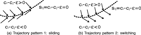
Two possible trajectory patterns at boundaries between subsystems

5.2 Trajectory Patterns at Boundaries Between the Subsystem and the BRUE Set
Since BRUE set is the fixed point set, the dynamic stays static within the BRUE set, i.e., \(\dot {\mathbf {x}}=0\). The boundary separating the BRUE set and one subsystems is: c i (x) − c j (x) = ε, while the subsystems adjacent to the BRUE set should be: c i (x) − c j (x) − ε > 0. The reason is: \(\mathbf {x} \notin \mathcal {X}_{BRUE}\), then \(\exists i \in \mathcal {A}\) such that \(x_{i}>0, c_{i}>\min _{j \in \mathcal { A}} c_{j}+\varepsilon \), indicating x is in the region where \(c_{i}(\mathbf {x})-c_{j}(\mathbf {x})-\varepsilon >0,\exists j\in \mathcal {A}, j\neq i\).
Based on the result in Section 5.1 and the property of the BRUE set, the trajectory which evolves from c i (x) − c j (x) − ε > 0 moves towards the boundary and then settle down at the boundary of the BRUE set (shown in Fig. 3).

Trajectory pattern at boundaries between subsystem and BRUE
The trajectory evolving within one subsystem will reach the boundary according to a LTI dynamic (as we mentioned in Section 4.2), so the boundary can be reached at an exponential rate.
5.3 Lyapunov Function Across Subsystems
Within each subsystem, the Lyapunov function is continuous with respect to time and the derivative of the Lyapunov function with respect to time is then calculated as:
where λ max(A q ) is the largest eigenvalue of the matrix A q . The last inequality is from the Rayleigh principle. As analyzed before, λ max(A q ) = 0. Thus, \(\dot {V}_{q}(x(t))\leqslant 0\).
We need to validate that the Lyapunov functions for sliding and switching decrease along the trajectory in both cases.
Case 1
(Sliding) The trajectory follows both dynamics in two adjacent subsystems \(\mathcal {X}_{1}: c_{p}-c_{j}-\varepsilon >0\) (i.e., link p is unacceptable) and \(\mathcal {X}_{2}: c_{p}-c_{j}-\varepsilon <0\) (i.e., link p is acceptable).
Assume the acceptable set of \(\mathcal {X}_{1}\) is a = {1, ⋯ ,p − 1}, and that of \(\mathcal { X}_{2}\) is a = {1, ⋯ ,p − 1,p}. Figure 4 illustrates the sliding mode between two subsystems. In the vicinity of the boundary s 12, both dynamics point towards the boundary. Therefore the trajectory evolves based on the combination of two dynamics, which behaves differently from that in a single subsystem.

Filippov Method for the sliding mode
The Filippov method (Filippov and Arscott 1988) is commonly used to describe this sliding mode precisely. According to Liberzon (2003), when decomposing the trajectory along two directions, there must exist a unique convex combination of f 1(x) and f 2(x) tangent to s 12 at the point x:
Let f 1(x) = β(u 1−x),f 2(x) = β(u 2−x). Then \(F(x)\,=\,\beta \left \lbrace \left [\alpha \mathbf {u}_{1}\,+\,(1\,-\,\alpha )\mathbf {u}_{2}\right ]-\mathbf {x}\left .\right \rbrace \right . \triangleq \beta \left (\mathbf {u}_{eq}-\mathbf {x}\right )\), where u eq =α u 1+(1−α)u 2.
Then the Lyapunov function for sliding is computed as:
In subsystem 1, link p is unacceptable: u 1−x =
In subsystem 2, link p is acceptable: u 2−x =
Then
Therefore the derivative of the Lyapunov function with respect to time is computed as:
where the first inequality is due to Eq. 5.1 and the second one is from Eq. 5.2 and negativity of Eq. 5.1.
Let \(W_{sliding}(\mathbf {x}(t))\triangleq -2\alpha (1-\alpha )\beta \left [ \frac {p+1}{p}\sum \limits _{k=p+1}^{n}{x_{k}^{2}}+\frac {1}{p}\sum \limits _{k=p+1}^{n}\sum \limits _{m=p+1}^{n}x_{k} x_{m}\right ]\). When \(\mathbf {x}\notin \mathcal {X}^{\varepsilon }_{BRUE}, \exists x_{k}, k=p+1,\cdots , n\) such that x k > 0. Therefore W sliding (x(t))>0. In summary, V(x(t + Δ t)) − V(x(t))⩽−W sliding (x(t))Δt for a small period Δt > 0. In other words, the changing rate of V along sliding is a negative function of the current system state x and is not zero unless \(\mathbf {x}\in \mathcal {X}^{\varepsilon }_{BRUE}\).
Case 2
(Switching) The trajectory changes direction and switches from subsystems \(\mathcal {X}_{1}: c_{p}(\mathbf {x})-c_{j}(\mathbf {x})-\varepsilon >0\) at \(t_{n_{i}}\) to \(\mathcal {X}_{2}: c_{p}(\mathbf {x})-c_{j}(\mathbf {x})-\varepsilon <0\) at \(t_{n_{i+1}}, t_{n_{i}}<t_{n_{i+1}}\) (See Fig. 5).

Switching mode
In subsystem 1, link p is unacceptable, then \(V_{1}(\mathbf {x}(t_{n_{i}})) = \frac {1}{2}\left [(p-1)^{2}\left (\frac {x_{p}+\sum \limits _{k=p+1}^{n}x_{k}}{p-1}\right )^{2} +{x_{p}^{2}}+\cdots +{x_{n}^{2}}\right ]\).
In subsystem 2, link p is acceptable, then \(V_{2}(\mathbf {x}(t_{n_{i+1}})) = \frac {1}{2}\left [p^{2}\left (\frac {\sum \limits _{k=p+1}^{n}x_{k}}{p}\right )^{2} +x_{p+1}^{2}+\cdots +{x_{n}^{2}}\right ]\).
The difference of these two function values is: \(V_{2}(\mathbf {x}(t_{n_{i+1}}))-V_{1}(\mathbf {x}(t_{n_{i}})) = -x_{p}\sum \limits _{k=p+1}^{n}x_{k}\). x p > 0 because link p is acceptable. When \(\mathbf {x}\notin \mathcal {X}^{\varepsilon }_{BRUE}, \exists x_{k}, k=p+1,\cdots , n\) such that x k > 0. Let \(W_{switch}(\mathbf {x}(t_{n_{i+1}})))\triangleq x_{p}\sum \limits _{k=p+1}^{n}x_{k}\). Then \(W(\mathbf {x}(t_{n_{i+1}})))>0\). Consequently \(V_{2}(\mathbf {x}(t_{n_{i+1}}))-V_{1}(\mathbf {x}(t_{n_{i}}))\leqslant -W_{switch}(\mathbf {x}(t_{n_{i+1}})))\). In other words, when the trajectory switches from \(\mathcal {X}_{1}\) to \(\mathcal { X}_{2}\), its Lyapnov function decreases abruptly. The difference of the two Lyapunov functions is a function of the current system state and will not be zero unless it is the BRUE.
According to the multiple Lyapunov method, we immediately have the following conclusion:
Proposition 5.1
Given a network with one OD pair connecting multiple links in parallel and the affine linear link function is strictly monotone and only dependent on its own flow, the BR dynamic is asymptotically stable.
5.4 Convergence of the BR Dynamic
Proposition 5.2
Given a network with one OD pair connecting multiple links in parallel and the affine linear link function is strictly monotone and only dependent on its own flow, the boundedly rational dynamic is convergent in finite time.
Proof
The trajectory patterns mentioned in Sections 5.1–5.2 show that trajectories can converge to the BRUE set by either sliding along the boundary or by evolving from one subsystem.
When sliding along the boundary to the BRUE set: the changing rate of the Lyapunov function in the sliding mode (defined in Eq. 5.3) depends on the system state, which is negative and bounded above, so the sliding mode can converge to the BRUE set in finite time.
When evolving from one subsystem to the BRUE set, at the boundaries between the subsystem and the BRUE set, \(V(\mathbf {x})>0, \dot {V}(\mathbf {x})<0, \mathbf {x} \in \partial \mathcal {X}\), and \(V(\mathbf {x}) = 0, \forall \mathbf {x} \in \mathcal {X}_{BRUE}\). The dynamic follows the LTI within the subsystem, so the BRUE set can be reached at an exponential rate. □
According to Proposition (5.1) and Proposition (5.2), we have the following conclusion:
Corollary 1
Given a network with one OD pair connecting multiple links in parallel and the affine linear link function is strictly monotone and only dependent on its own flow, the boundedly rational dynamic is stable.
Remark
For the continuous-time BR dynamic, if the initial dynamic starts from outside the BRUE set, trajectories will remain static once it reaches the boundaries of the BRUE set. Therefore the interior of the BRUE set will never be reached.
6 Stability Analysis on a Small Network
The one OD pair with three links example in Guo and Liu (2011) is used to illustrate the stability analysis. A three-link network with one OD pair of demand 50, the link cost for each link is 30+x 1, 30+3x 2, 30+3x 3. Since the link is the path, so we will use the link cost and link flow in the subsequent analysis. The indifference bound ε = 10.
As a common tool in studying the stability of a dynamical system, the phase portrait graph is plotted in Fig. 6, depicting the link flow trajectories with arrows and stable steady states with dots. Arrows mean the direction where the trajectory evolves if it passes the ending point of the arrow; while dots represent that all the trajectories stop there and reach the equilibrium state.

Phase portrait of the BR dynamic
In Fig. 6, the horizontal line is the flow on link 1, while the vertical one is the flow on link 2. The big triangle region encompassed by the diagonal line and the axes are the feasible link flow set. The hexahedron in the middle is the BRUE set, and the phase portrait becomes dots inside the BRUE set. Each blue arrow represents the changing direction of the point located at the end of the arrow. Based on where these blue arrows point to, we can see six distinct patterns, dividing the feasible link flow set into six subsystems. There are two types of subsystems: the triangle one (numbered 1,2,3 in red) and the non-convex one (numbered 4,5,6 in red). Each subsystem corresponds to a different acceptable path flow set. For instance, in subsystem (1), only path 1 is acceptable; while in subsystem (4), both path 2 and 3 are acceptable.
There are six discontinuity boundaries separating these subsystems: c i (x) − c j (x) − ε = 0, i, j = 1, 2, 3, i ≠ j, indicated in black color. The trajectories close to them behave in two different ways: (1) i = 1,j = 2 or 3: the trajectories close to one side of the discontinuity surface are likely to reach it, while those starting from the other side will evolve to the opposite direction and directly converge to the equilibria; (2) i = 2 or 3,j = 1 or i = 2,j = 3: the trajectories close to both sides will reach them.
Figure 7 indicates the Lyapnov function defined in the feasible link set. The color shows the value of the Lyapnov function evaluated at each flow pattern: The darker the color is, the higher the Lyapnov value is. The middle of the figure is the BRUE set, which has zero Lyapnov value, so this set is the lowest region. Outside the BRUE set, the Lyapnov function is greater than zero, so other regions have higher elevation. We can see clearly that, Lyapnov function is a piece-wise function, with each piece defined in the partition the same as that in Fig. 6. This observation is consistent with the property of the Lyapnov function that, Lyapnov function is continuous within each subsystem, but discontinuous on boundaries. Regarding each piece, it is lowering down towards the BRUE set.

Lyapunov function
As mentioned before, There are two trajectory patterns in the BR dynamic. To illustrate how different trajectories evolve with time, we plot these two typical trajectories in Fig. 6 in green lines. The number of each trajectory is marked on the right side of its starting point.
Two green lines represent two trajectories starts from arbitrary initial points and then evolves with time, according to the BR dynamic. Trajectory 1 starts close to the sliding line c 2(x) − c 1(x) = ε and reaches it very quickly, then slides along it to the BRUE. By contrast, c 1(x) − c 2(x) = ε is also a discontinuity surface separating two different regions. However, when trajectory 2 touches this discontinuity surface, it does not stay on it. Instead, its direction gets changed abruptly and then converge to the BRUE set from the other subregion.
In Fig. 8a–b the horizontal axis is the time, and the vertical axis is the Lyapnov function along the trajectory. The red number in the box indicates in which subsystem this trajectory is evolving during that time period.

Lyapunov function along the trajectory. a Trajectory 1. b Trajectory 2
In Fig. 8a, ‘4/1’ means the trajectory is sliding along the boundary between subsystem 1 and 4. The Lyapnov function is decreasing gradually, and suddenly drop to zero when it reaches the equilibrium. In Fig. 8b, the Lyapnov function is decreasing in each region, and has a sudden drop when the trajectory switches from subsystem 2 to 4, and another drop when the equilibrium is attained. Figure 8a–b have different time scales, because it takes longer time for sliding dynamic to reach the equilibrium.
We can also explain why trajectory 1 and 2 have such a distinct pattern by inspecting Fig. 7. The Lyapunov function represents the potential energy of the BR dyanmical system, and the BRUE set has the lowest energy. The trajectory has the tendency to move to the lower energy region.
7 Conclusion and Future Work
This paper provided a methodology of proving the stability of the boundedly rational (BR) day-to-day dynamic proposed by Guo and Liu (2011). It first reduced the bounded ration (BR) dynamic to a piecewise affine linear system composed of multiple subsystems and then gave rigorous proofs of the stability property of the BR dynamic.
Due to non-uniqueness of the equilibria and the state-dependent structure of the BR dynamic, the methodology of proving the stability is different from the conventional Lyapunov Theorem used in some day-to-day literature. In this study, we employed the multiple Lyapunov method specially proposed for the hybrid dynamical system. This method requires that different Lyapunov functional forms are defined among subsystems. If the Lyapunov values always decrease along trajectories, then the dynamical system is stable. As this method is initially proposed for the dynamical systems with a single fixed point while the BR dynamic has multiple equilibria, we first showed that the boundedly rational user equilibria set (i.e., the fixed points of the BR dynamic) is connected and thus the trajectories of the BR dynamic can only converge to this set.
By defining the Lyapunov function as the distance between the current flow and its acceptable path set, we proved that this Lyapunov function decreases within each subsystem at an exponential rate. When trajectories reach boundaries between subsystems, they can either slide or switch. We also showed that the Lyapunov function drops in these two cases. In summary, the BR dynamic is stable and trajectories are convergent in finite time.
Although this study proved the stability of the BR dynamic, it has been limited by the underlying assumptions of linear and separable link performance functions. Thus, the stability property of a BR dynamic with nonlinear cost functions needs to be analyzed in the future. In addition, we should extend the stability analysis to general networks with multiple OD pairs.
References
Blondel V, Tsitsiklis J (1999) Complexity of stability and controllability of elementary hybrid systems. Automatica 35:479–490
Branicky M (1998) Multiple Lyapunov functions and other analysis tools for switched and hybrid systems. IEEE Trans Autom Control 43(4):475–482
Cantarella GE, Gentile G, Velonà P (2010) Uniqueness of stochastic user equilibrium. In: Proceedings of 5th IMA conference on mathematics in transportation, London
Cantarella GE, Velonà P, Watling DP (2013) Day-to-day dynamics & equilibrium stability in a two-mode transport system with responsive bus operator strategies. Netw Spat Econ 1–22
Di X, Liu HX, Pang J-S, Ban X (2013) Boundedly rational user equilibria (BRUE): mathematical formulation and solution sets. Transp Res B. doi:10.1016/j.trb.2013.06.008
Filippov A, Arscott F (1988) Differential equations with discontinuous righthand sides, vol 18. Springer
Friesz T, Bernstein D, Mehta N, Tobin R, Ganjalizadeh S (1994) Day-to-day dynamic network disequilibria and idealized traveler information systems. Oper Res 42(6):1120–1136
Guo X, Liu H (2011) Bounded rationality and irreversible network change. Transp Res B 45(10):1606–1618
Han L, Du L (2012) On a link-based day-to-day traffic assignment model. Transp Res B 46(1):72–84
He X (2010) Modeling the traffic flow evolution process after a network disruption. Ph.D. thesis, University of Minnesota
He X, Guo X, Liu H (2010) A link-based day-to-day traffic assignment model. Transp Res B 44(4):597–608
Hu T, Mahmassani H (1997) Day-to-day evolution of network flows under real-time information and reactive signal control. Transp Res C 5(1):51–69
LaValle SM (2006) Planning algorithms. Cambridge University Press
Liberzon D (2003) Switching in systems and control. Springer
Lou Y, Yin Y, Lawphongpanich S (2010) Robust congestion pricing under boundedly rational user equilibrium. Transp Res B 44(1):15–28
Mahmassani H, Chang G (1987) On boundedly rational user equilibrium in transportation systems. Transp Sci 21(2):89–99
Mahmassani H, Liu Y (1999) Dynamics of commuting decision behaviour under advanced traveller information systems. Transp Res C 7(2–3):91–107
Mignone D, Ferrari-Trecate G, Morari M (2000) Stability and stabilization of piecewise affine and hybrid systems: An LMI approach In: Proceedings of the 39th IEEE Conference on Decision and Control, 2000, vol 1. IEEE, pp 504–509
Nagurney A, Zhang D (1997) Projected dynamical systems in the formulation, stability analysis, and computation of fixed-demand traffic network equilibria. Transp Sci 31(2):147–158
Simon H (1955) A behavioral model of rational choice. Q J Econ 69(1):99–118
Smith M (1979) The existence, uniqueness and stability of traffic equilibria. Transp Res B 13(4):295–304
Smith M (1984) The stability of a dynamic model of traffic assignment–an application of a method of Lyapunov. Transp Sci 18(3):245–252
Szeto W, Lo H (2006) Dynamic traffic assignment: properties and extensions. Transportmetrica 2(1):31–52
Szidarovszky F (1998) Linear systems theory. CRC press
Terrell WJ (2009) Stability and stabilization: an introduction. Princeton University Press
Watling D (1999) Stability of the stochastic equilibrium assignment problem: a dynamical systems approach. Transp Res B 33(4):281–312
Watling D, Hazelton M (2003) The dynamics and equilibria of day-to-day assignment models. Netw Spat Econ 3(3):349–370
Watling DP, Cantarella GE (2013) Modelling sources of variation in transportation systems: theoretical foundations of day-to-day dynamic models. Transportmetrica B: Transp Dyn 1(1):3–32
Acknowledgments
This research was funded by the National Science Foundation (EFRI-1024604 and EFRI-1024647. The first author would like to thank Professor Cantarella from the University of Salerno for his precious comments on extending the multiple Lyapunov method which was proposed for a single fixed point to showing the stability of a dynamic with non-unique fixed points.
Author information
Authors and Affiliations
Corresponding author
Rights and permissions
About this article

Cite this article
Di, X., Liu, H.X., Ban, X.(.X. et al. Submission to the DTA 2012 Special Issue: On the Stability of a Boundedly Rational Day-to-Day Dynamic. Netw Spat Econ 15, 537–557 (2015). https://doi.org/10.1007/s11067-014-9233-y
Published:
Issue Date:
DOI: https://doi.org/10.1007/s11067-014-9233-y