Self-assembly of discrete self-similar fractals

Abstract

In this paper, we search for theoretical limitations of the Tile Assembly Model (TAM), along with techniques to work around such limitations. Specifically, we investigate the self-assembly of fractal shapes in the TAM. We prove that no self-similar fractal weakly self-assembles at temperature 1 in a locally deterministic tile assembly system, and that certain kinds of discrete self-similar fractals do not strictly self-assemble at any temperature. Additionally, we extend the fiber construction of Lathrop et al. (2009) to show that any discrete self-similar fractal belonging to a particular class of “nice” discrete self-similar fractals has a fibered version that strictly self-assembles in the TAM.

1 Introduction

Self-assembly is a bottom-up process by which (usually a small number of) fundamental components automatically coalesce to form a target structure. In 1998, Winfree (1998) introduced the (abstract) Tile Assembly Model (TAM)—an effective version of Wang tiling (Wang 1961, 1963)—and a mathematical model of DNA self-assembly pioneered by Seeman (1982). In the TAM, the fundamental components are un-rotatable, but translatable “tiles” whose sides are labeled with glue “colors” and “strengths.” Two tiles that are placed next to each other interact if the glue colors on their abutting sides match, and they bind if the strength on their abutting sides matches and is at least as great as a given “temperature” value. Rothemund and Winfree (2001, 2000) later refined the model, and Lathrop et al. (2009) gave a treatment of the TAM in which equal status is bestowed upon the self-assembly of infinite and finite structures. There are also several generalizations (Aggarwal et al. 2004; Kao and Schweller 2007; Majumder et al. 2007) of the TAM.

Despite its deliberate over-simplification, the TAM is a computationally and geometrically expressive model. For instance, Winfree (1998) proved that the TAM is computationally universal, and thus can be directed algorithmically. Winfree (1998) also exhibited a seven-tile-type self-assembly system, directed by a clever XOR-like algorithm, that “paints” a picture of a well-known shape, the discrete Sierpinski triangle S, onto the first quadrant. Note that the underlying shapes of each of the previous results are infinite canvases that cover the first quadrant, onto which computationally interesting shapes are painted (in Lathrop et al. 2009, this is defined as weak self-assembly). Moreover, Lathrop et al. (2008) recently gave a characterization of the computably enumerable languages in terms of weak self-assembly using a “2-dimensional ray construction” in which, for any TM M, a “quadratically spaced out” version of the projection of L(M) along the positive x-axis weakly self-assembles.

Strict self-assembly is the self-assembly of a particular connected shape and nothing else. Note that strict self-assembly is a special case of weak self-assembly, where the underlying canvas (onto which a shape $X \subseteq {\mathbb{Z}}^2$ is painted) is the shape X itself. We say that the tile complexity of a shape X is the size of the tile set in which X strictly self-assembles. For the case of the strict self-assembly of finite shapes, the tile complexity of the shape becomes an important factor because every finite shape trivially (but perhaps not feasibly) strictly self-assembles via a spanning-tree construction. Numerous lower bounds on the tile complexity for the strict self-assembly of particular classes of shapes have been established. For instance, Rothemund and Winfree (2000) proved that there exist very small tile sets in which extremely large squares strictly self-assemble. In 2002, Adleman et al. (2002) exhibited polynomial-time algorithms capable of finding the “minimum” tile assembly system (with respect to tile complexity) in which tree shapes and squares strictly self-assemble. Moreover, Soloveichik and Winfree (2007) discovered the remarkable fact that, if one is not concerned with the scale of an “algorithmically describable” finite shape X, then there is always a small tile set in which X strictly self-assembles.

For the case of strict self-assembly of infinite shapes, the power of the TAM has only recently been investigated. In this case, we ignore tile-complexity and are thus primarily concerned with the question of whether or not there is any tile assembly system in which a particular infinite shape strictly self-assembles. Note that, unlike for the case of the strict self-assembly of finite shapes, the tile complexity of an infinite shape X cannot be a function of |X|. Much of the previous work in this area has focused on the strict self-assembly of discrete fractal structures. In particular, Lathrop et al. (2009) established that self-similar tree shapes do not strictly self-assemble in the TAM. A “fiber construction” is also given in Lathrop et al. (2009), in which a non-trivial (infinite) fractal structure resembling the standard discrete Sierpinski triangle strictly self-assembles. Moreover, Kautz and Lathrop (2009) define an infinite class of “numerically self-similar” discrete self-similar fractals (to which the Sierpinski triangle and the Sierpinski carpet belong), and give a general construction for generating tile assembly systems in which such numerically self-similar fractals weakly self-assemble.

In this paper, we search for (1) theoretical limitations of the TAM, with respect to the strict self-assembly of infinite shapes, and (2) techniques that allow one to “work around” such limitations. Specifically, we investigate the strict self-assembly of fractal shapes in the TAM. We are interested in fractal shapes because of their geometric aperiodicity and their frequent occurrence in natural biological systems. We prove three main results: two negative and one positive. Our first negative (i.e., impossibility) result says that no self-similar fractal weakly self-assembles in the TAM at temperature 1 in a locally deterministic tile assembly system. In our second impossibility result, we exhibit a class of discrete self-similar fractals, to which the standard discrete Sierpinski triangle belongs, that do not strictly self-assemble in the TAM (at any temperature). Finally, in our positive result, we use simple modified counters to extend the fiber construction from Lathrop et al. (2009) to a particular class of “nice” discrete self-similar fractals.

2 Preliminaries

2.1 The Tile Assembly Model

We work in the 2-dimensional discrete Euclidean space ${\mathbb{Z}}^2.$ We write U ₂ for the set of all unit vectors, i.e., vectors of length 1, in ${\mathbb{Z}}^2.$ We regard the 4 elements of U ₂ as (names of the cardinal) directions in ${\mathbb{Z}}^2.$

We now give a brief and relatively self-contained introduction to the abstract Tile Assembly Model that is adequate for reading this paper. More formal details and discussion may be found in Lathrop et al. (2009), Rothemund (2001), Rothemund and Winfree (2000), and Winfree (1998). Our notation is that of Lathrop et al. (2009).

A grid graph is a graph G = (V, E) in which $V \subseteq {\mathbb{Z}}^2$ and every edge $\{\vec{a}, \vec{b} \} \in E$ has the property that $\vec{a} - \vec{b} \in U_2.$ The full grid graph on a set $V \subseteq {\mathbb{Z}}^2$ is the graph G ^# _V = (V, E) in which E contains every $\{\vec{a}, \vec{b} \} \in [V]^2$ such that $\vec{a} - \vec{b} \in U_2.$ Intuitively, a tile type t is a unit square that can be translated, but not rotated, so it has a well-defined “side $\vec{u}$” for each $\vec{u} \in U_2.$ Each side $\vec{u}$ is covered with a “glue” of “color” $\hbox{col}_t(\vec{u})$ and “strength” $\hbox{str}_t(\vec{u})$ specified by its type t. Tiles are depicted as squares whose various sides have a dashed line, one solid line, or two solid lines, indicating whether the glue strengths on these sides are 0, 1, or 2, respectively. Thus, for example, a tile of the type shown in Fig. 1 has glue of strength 0 on the left and bottom, glue of color ‘A’ and strength 1 on the top, and glue of color ‘B’ and strength 2 on the right. This tile also has a label ‘L’, which plays no formal role.

Fig. 1

Example tile type

Two tiles t and t′ that are placed at the points $\vec{a}$ and $\vec{a}+\vec{u}$ respectively, bind with strength $\hbox{str}_t\left(\vec{u}\right)$ if and only if $\left(\hbox{col}_t\left(\vec{u}\right),\hbox{str}_t\left(\vec{u}\right)\right) =\left(\hbox{col}_{t'}\left(-\vec{u}\right),\hbox{str}_{t'}\left(-\vec{u}\right)\right).$ In this paper, all glues have strength 0, 1, or 2. Each side’s “color” is indicated by an alphanumeric label. An example of a tile set is shown in Figs. 2, 3. Given a set T of tile types and a “temperature” $\tau \in {\mathbb{N}},$ a τ-T-assembly is a partial function $\alpha:{{\mathbb{Z}}^2}\dashrightarrow{T}$ -intuitively, a placement of tiles at some locations in ${\mathbb{Z}}^2.$ The binding graph of an assembly α is the grid graph G _α = (V, E), where V =  dom α, and $\{\vec{m}, \vec{n}\} \in E$ if and only if (1) $\vec{m} - \vec{n} \in U_2,$ (2) $\hbox{col}_{\alpha(\vec{m})}\left(\vec{n} - \vec{m}\right) = \hbox{col}_{\alpha(\vec{n})}\left(\vec{m} - \vec{n}\right),$ (3) $\hbox{str}_{\alpha(\vec{m})}\left(\vec{n} - \vec{m}\right) = \hbox{str}_{\alpha(\vec{n})}\left(\vec{m} - \vec{n}\right),$ and (4) $\hbox{str}_{\alpha(\vec{m})}\left(\vec{n} -\vec{m}\right) > 0.$ An assembly is τ-stable, if it cannot be broken up into smaller assemblies without breaking bonds of total strength at least τ (i.e., if every cut of G _α cuts edges, the sum of whose strengths is at least τ). For each $t \in T,$ the τ-t-frontier of α, written as ∂^τ _t α, is the set of all locations to which t can be τ-stably added to α. For each $t \in T,$ we write ∂ _t α for the set of all locations to which a tile of type t can be τ-stably added. We write ∂α for the set of all locations to which some tile can be τ-stably added to α. We refer to ∂α as the frontier of α. If α and α′ are assemblies, then α is a subassembly of α′, and we write $\alpha\,\sqsubseteq\,\alpha',$ if $\hbox{dom}\,{\alpha} \subseteq \hbox{dom}\,{\alpha'}$ and $\alpha(\vec{m}) = \alpha'(\vec{m})$ for all $\vec{m} \in \hbox{dom}\,{\alpha}.$

Fig. 2

Example tile set

Fig. 3

Example 2-T-assembly, where T is the tile set shown in Fig. 2. Note that the size of the frontier of this assembly is 1

Self-assembly begins with a seed assembly σ and proceeds asynchronously and nondeterministically, with tiles adsorbing one at a time to the existing assembly in any manner that preserves τ-stability at all times. A tile assembly system (TAS) is an ordered triple ${\mathcal{T}} = (T, \sigma, \tau),$ where T is a finite set of tile types, σ is a seed assembly with finite domain, and $\tau \in {\mathbb{N}}.$ A generalized tile assembly system (GTAS) is defined similarly, but without the finiteness requirements. An assembly sequence in a TAS ${\mathcal{T}}$ is a (finite or infinite) sequence $\vec{\alpha} = (\alpha_0,\alpha_1,\ldots)$ of assemblies in which each α_i+1 is obtained from α _i by the addition of a single tile. The result $\hbox{res}({\vec{\alpha}})$ of such an assembly sequence is its unique limiting assembly (This is the last assembly in the sequence if the sequence is finite). Figures 4, 5 shows an example of a 2-T-assembly sequence (where T is the tile set shown in Fig. 2), with its result being the right most assembly.

Fig. 4

An example assembly sequence with respect to the tile set shown in Fig. 2

Fig. 5

An example of a 2-T-assembly that is terminal, where T is the tile set shown in Fig. 2

We write ${\mathcal{A}}[{\mathcal{T}}]$ for the set of all assemblies that can arise via some assembly sequence in ${\mathcal{T}}.$ An assembly α is terminal, and we write $\alpha \in {\mathcal{A}}_{\square}[{\mathcal{T}}],$ if no tile can be τ-stably added to it. The set ${\mathcal{A}}[{\mathcal{T}}]$ is partially ordered by the relation $\longrightarrow$ defined by

$$ \begin{array}{lll} \alpha \longrightarrow \alpha' &\Leftrightarrow & \hbox{there is an assembly} \cr &&\hbox{sequence}\,\vec{\alpha} = (\alpha_0,\alpha_1,\ldots) \cr &&\hbox{such that}\,\alpha_0 = \alpha\,\hbox{and} \cr && \alpha' =\hbox{res}({\vec{\alpha}}). \end{array} $$

We say that ${\mathcal{T}}$ is directed if the relation $\longrightarrow$ is directed, i.e., if for all $\alpha,\alpha' \in {\mathcal{A}}[{\mathcal{T}}],$ there exists $\alpha'' \in {\mathcal{A}}[{\mathcal{T}}]$ such that ${\alpha}{\longrightarrow}\alpha''$ and ${\alpha'}\longrightarrow \alpha''.$ It is easy to show that ${\mathcal{T}}$ is directed if and only if there is a unique terminal assembly $\alpha \in {\mathcal{A}}[{\mathcal{T}}]$ such that ${\sigma}{\longrightarrow}\alpha.$ The reader is cautioned that the term “directed” has also been used for a different, more specialized notion in self-assembly (Adleman et al. 2002). We interpret “directed” to mean “deterministic”, though there are multiple senses in which a TAS may be deterministic or nondeterministic.

A set $X \subseteq {\mathbb{Z}}^2$ weakly self-assembles if there exists a TAS $\mathcal{T} = (T, \sigma, \tau)$ and a set $B \subseteq T$ (B constitutes the “black” tiles) such that α⁻¹(B) = X holds for every assembly $\alpha \in {\mathcal{A}}_{\square}[{\mathcal{T}}].$ A set X strictly self-assembles if there is a TAS ${\mathcal{T}}$ for which every assembly $\alpha\in{\mathcal{A}}_{\square}[{\mathcal{T}}]$ satisfies dom  α = X. Note that if X strictly self-assembles, then X weakly self-assembles. (Let all tiles be black.)

For the sake of example, let ${\mathcal{T}} = (T,\sigma,2)$ be the tile assembly system where T is the set of tile types given in Fig. 2 and σ is an assembly such that σ(0,0) = t, where $t \in T$ is the unique tile type with the label ‘1’ (and undefined elsewhere). Then it is clear that the set

$$ X = \{(0,0),(1,0),(2,0),(0,1),(1,1),(2,1)\} $$

strictly self-assembles in ${\mathcal{T}}.$ Furthermore, if we define the set B of “black” tiles to be the singleton set containing the tile type labeled ‘5’, then it follows that the set

$$ Y = \{(0,1),(1,1)\} $$

weakly self-assembles in ${\mathcal{T}}.$

2.2 A brief sketch of local determinism

Our first main theorem uses local determinism (Soloveichik and Winfree 2007), which we now briefly review.

Notation 2.1

For each assembly α, each $\vec{m} \in {\mathbb{Z}}^2,$ and each $\vec{u} \in U_2,$

$$ \hbox{str}_{\alpha}(\vec{m},\vec{u}) = \hbox{str}_{\alpha(\vec{m})}(\vec{u})\cdot \left[\left[\alpha(\vec{m})(\vec{u}) = \alpha(\vec{m}+\vec{u})(-\vec{u})\right]\right], $$

where [[ϕ]] is the Boolean value of the statement ϕ. The Boolean value on the right is 0 if $\{\vec{m},\vec{m}+\vec{u}\} \nsubseteq\,\hbox{dom}\,{\alpha}.$

Notation 2.2

If $\vec{\alpha} = (\alpha_i \mid 0\leq\,i\,<\,k)$ is an assembly sequence in the TAS ${\mathcal{T}} = (T,\sigma,\tau),$ and $\vec{m} \in {\mathbb{Z}}^2,$ then the $\vec{\alpha}$ -index of $\vec{m}$ is

$$ i_{\vec{\alpha}}(\vec{m}) = \min\{i\in {\mathbb{N}} \; \left| \; \vec{m} \in \hbox{dom}\,{\alpha_i} \right. \}. $$

Observation 2.3

$\vec{m} \in \hbox{dom}\,{\hbox{res}({\vec{\alpha}})} \Leftrightarrow i_{\vec{\alpha}}(\vec{m}) < \infty.$

Notation 2.4

If $\vec{\alpha} = (\alpha_i \mid 0\leq\, i\,<\,k)$ is an assembly sequence in the TAS ${\mathcal{T}} = (T,\sigma,\tau),$ then, for $\vec{m},\vec{m}' \in {\mathbb{Z}}^2,$

$$ \vec{m} \prec_{\vec{\alpha}} \vec{m}' \Leftrightarrow i_{\vec{\alpha}}(\vec{m}) < i_{\vec{\alpha}}(\vec{m}'). $$

Definition 2.5

(Soloveichik and Winfree 2007) Let $\vec{\alpha} = (\alpha_i \mid 0\leq i < k)$ be an assembly sequence in the TAS ${\mathcal{T}} = (T,\sigma,\tau),$ and let $\alpha = \hbox{res}({\vec{\alpha}}).$ For each location $\vec{m} \in \hbox{dom}\,{\alpha},$ define the following sets of directions.

• 1. $\hbox{IN}^{\vec{\alpha}}(\vec{m}) = \left\{\vec{u} \in U_2 \; \left| \; \vec{m}+\vec{u} \prec_{\vec{\alpha}} \vec{m} \hbox{ and } \hbox{str}_{\alpha_{i_{\vec{\alpha}}(\vec{m})}}(\vec{m},\vec{u})>0 \right.\right\}.$

• 2. $\hbox{OUT}^{\vec{\alpha}}(\vec{m}) = \left\{\vec{u}\in U_2 \; \left| \; -\vec{u} \in \hbox{IN}^{\vec{\alpha}}(\vec{m}+\vec{u} \right.) \right\}.$

Intuitively, $\hbox{IN}^{\vec{\alpha}}(\vec{m})$ is the set of sides on which the tile at $\vec{m}$ initially binds in the assembly sequence $\vec{\alpha},$ and $\hbox{OUT}^{\vec{\alpha}}(\vec{m})$ is the set of sides on which this tile propagates information to future tiles. Note that $\hbox{IN}^{\vec{\alpha}}(\vec{m}) = \emptyset$ for all $\vec{m} \in \alpha_0.$

Notation 2.6

If $\vec{\alpha} = (\alpha_i \mid 0 \leq i < k)$ is an assembly sequence in the TAS ${\mathcal{T}} = (T,\sigma,\tau), \alpha = \hbox{res}({\vec{\alpha}}),$ and $\vec{m} \in \hbox{dom}\,{\alpha} - \hbox{dom}\,{\alpha_0},$ then

$$ \vec{\alpha} \setminus \vec{m} = \alpha \upharpoonright \left(\hbox{dom}\,{\alpha} - \{\vec{m}\} - \left(\vec{m}+\hbox{OUT}^{\vec{\alpha}}(\vec{m})\right)\right). $$

(Note that $\vec{\alpha} \setminus \vec{m}$ may or may not be a stable assembly.)

Definition 2.7

(Soloveichik and Winfree 2007). An assembly sequence $\vec{\alpha} = (\alpha_i \mid 0 \leq i < k)$ in the TAS ${\mathcal{T}} = (T,\sigma,\tau),$ with result α is locally deterministic if it has the following three properties.

• 1. For all $\vec{m} \in \hbox{dom}\,{\alpha} - \hbox{dom}\,{\alpha_0},$

  $$ \sum_{\vec{u} \in \hbox{IN}^{\vec{\alpha}}(\vec{m})}{\hbox{str}_{\alpha_{i_{\vec{\alpha}} (\vec{m})}}(\vec{m},\vec{u}) } = \tau. $$

• 2. For all $\vec{m} \in \hbox{dom}\,{\alpha} - \hbox{dom}\,{\alpha_0}$ and all $t \in T-\{\alpha(\vec{m})\}, \vec{m} \notin \partial _{t}^{\tau}{\left(\vec{\alpha} \setminus \vec{m}\right)}.$

• 3. $\alpha \in {\mathcal{A}}_{\square}[{\mathcal{T}}].$

Intuitively, $\vec{\alpha}$ is locally deterministic if (1) each tile added in $\vec{\alpha}$ “just barely” binds to the assembly; (2) if a tile of type t ₀ at a location $\vec{m}$ and its immediate “OUT-neighbors” are deleted from the result of $\vec{\alpha},$ then no tile of type $t \ne t_0$ can attach itself to the thus-obtained configuration at location $\vec{m};$ and (3) the result of $\vec{\alpha}$ is terminal. See Fig. 4 for an example of a locally deterministic assembly sequence.

Definition 2.8

A TAS ${\mathcal{T}} = (T,\sigma,\tau)$ is locally deterministic if there exists a locally deterministic assembly sequence $\vec{\alpha}=(\alpha_i \mid 0\leq i < k)$ with α₀ = σ.

Lemma 2.9

(Soloveichik and Winfree 2007) If the TAS ${\mathcal{T}} = (T,\sigma,\tau)$ is locally deterministic, then every assembly sequence $\vec{\alpha} = (\alpha_i \mid 0 \leq i < k)$ in ${\mathcal{T}}$ is locally deterministic.

Theorem 2.10

(Soloveichik and Winfree 2007) Every locally deterministic TAS is directed.

2.3 Discrete self-similar fractals

In this subsection we introduce discrete self-similar fractals, and a kind of discrete fractal dimension called zeta-dimension (Doty et al. 2005).

Definition 2.11

Let $1 < c \in {\mathbb{N}},$ and $X\,\subsetneq\,{\mathbb{N}}^2$ (we do not consider ${\mathbb{N}}^2$ to be a self-similar fractal). We say that X is a c-discrete self-similar fractal, if there is a set $V \subseteq \{0,\ldots,c-1\}\times\{0,\ldots,c-1\}$ with |V| > c, and

$$ V \not \in \left\{\{(i,i) \mid 0 \leq i < c\}, \{(i,0) \mid 0 \leq i < c \}, \{(0,i) \mid 0 \leq i < c\}\right\}, $$

such that

$$ X = \bigcup_{i=0}^{\infty}{X_i}, $$

where X _i is the ith stage satisfying X ₀ =  {(0,0)}, and X _i+1 = X _i  ∪ (X _i  + c ⁱ V). In this case, we say that V generates X.

Intuitively, we define c-discrete self-similar fractals as follows (demonstrated in Fig. 6). Begin with a c x c square where the 0th stage is defined simply by the point (0,0). The first stage, which we call the generator is defined by selecting additional locations in the c x c square. Every subsequent stage i is formed by treating the stage i−1 as a magnified version of the point (0,0) in the generator and creating one full copy of stage i−1 for every other point in the generator, then treating those copies as the magnified versions of their respective points in the generator and translating them accordingly.

Fig. 6

The first four stages of the discrete Sierpinski carpet (X ₀, X ₁ = V, X ₂, and X ₃ are shown in (a), (b), (c), and (d) respectively)

Definition 2.12

$X\,\subsetneq\, {\mathbb{N}}^2.$ We say that X is a discrete self-similar fractal if it is a c-discrete self-similar fractal for some $c \in {\mathbb{N}}.$

In this paper, we are concerned with the following class of self-similar fractals.

Definition 2.13

A nice discrete self-similar fractal is a discrete self-similar fractal such that $(\{0,\ldots,c-1\} \times \{0\}) \cup (\{0\}\times\{0,\ldots,c-1\}) \subseteq V,$ and G ^# _V is connected.

See Fig. 7 for examples of nice discrete self-similar fractals.

Fig. 7

The generators of discrete self-similar fractals. The fractals in (a) are nice, whereas (b) shows two non-nice fractals

The most commonly used dimension for discrete fractals is zeta-dimension, which we use in this paper.

Definition 2.14

(Doty et al. 2005) For each set $A \subseteq {\mathbb{Z}}^2,$ the zeta-dimension of A is

$$ \hbox{Dim}_{\zeta}(A) = \limsup_{n \rightarrow \infty}{\frac{\log|A_{\le n}|}{\log n}}, $$

where $A_{\le n} = \{(k,l) \in A \mid |k|+|l| \le n\}.$

It is clear that 0 ≤ Dim_ζ(A) ≤ 2 for all $A \subseteq {\mathbb{Z}}^2.$

3 Impossibility results

In this section, we explore the theoretical limitations of the Tile Assembly Model with respect to the self-assembly of fractal shapes. We are specifically interested in the self-assembly of discrete fractal structures because of their geometrically aperiodic structure. First, we establish that no discrete self-similar fractal weakly self-assembles at temperature τ = 1 in a locally deterministic tile assembly system. Second, we exhibit a class ${\mathcal{C}}$ of discrete self-similar fractals, and prove that if $F \in {\mathcal{C}},$ then F does not strictly self-assemble in the TAM.

Throughout this section, we assume (without loss of generality) that T is a finite set of tile types, and σ is an assembly that places a single tile at the origin.

The following theorem is evidence in support of the claim that locally deterministic temperature 1 tile assembly systems cannot produce “sophisticated” shapes and patterns.

Theorem 3.1

Let${\mathcal{T}} = (T,\sigma,\tau = 1)$be a tile assembly system, and$\alpha \in {\mathcal{A}}_{\square}[{\mathcal{T}}].$If${\mathcal{T}}$is locally deterministic, then the binding graphG_αis a tree.

Proof

Suppose that the binding graph G _α is not a tree. Then there is a cycle C in G _α. Let $\vec{z} \in C, t = \alpha(\vec{z})$ and $\vec{\alpha}$ be an assembly sequence satisfying $\alpha = \hbox{dom}\,{\hbox{res}({\vec{\alpha}})}.$ There must be two simple paths π₁ and π₂ in G _α from $\vec{0}$ to $\vec{z}$ with π₁≠π₂. Since τ = 1, there exists an assembly sequence $\vec{\alpha}'$ where $\vec{\alpha}'$ first assembles $\pi_1 \cap \pi_2$ (if such an intersection exists), then assembles $(\pi_1 - \pi_2) - \{\vec{z}\},$ and finally assembles $(\pi_2 - \pi_1) - \{\vec{z}\}.$ We can use $\vec{\alpha}'$ to define the assembly sequence $\vec{\alpha}''$ that does what $\vec{\alpha}'$ does but places the tile type t at position $\vec{z}$ and then does whatever $\vec{\alpha}$ does for all $\vec{m} \not \in \hbox{dom}\,{\hbox{res}({\vec{\alpha}'})}.$ But since $\vec{z} \in C,$ the tile that $\vec{\alpha}'$ places at position $\vec{z}$ has two input sides and binds with strength 2 > τ = 1. Thus, the assembly sequence $\vec{\alpha}'$ is not locally deterministic, and it follows by Lemma 2.9 that ${\mathcal{T}}$ is not locally deterministic. □

See Fig. 8 for a visual depiction of the above proof.

Fig. 8

Visual depiction of the proof of Lemma 3.1. If a cycle could exist (image a), then image b shows a possible partial assembly to which the tile attaching in location $\vec{z}$ would bind with strength 2. This is a contradiction to the claim that the tile assembly system is temperature one and locally deterministic. a An example of a cycle existing in the binding graph of an assembly; b A possible partial assembly which forms both paths to $\vec{z}$ before $\vec{z}$ is tiled

Note that the converse of Theorem 3.1 is not necessarily true.

Definition 3.2

(Lathrop et al. 2009) Let G = (V,E) be a graph, and let $D \subseteq V.$ For each $r \in V,$ the D-r-rooted subgraph of G is the graph G _D,r = (V _D,r, E _D,r ), where

$$ V_{D,r} = \left\{v \in V \left| \hbox{every\,simple\,path\,from\,} v \,\hbox{to}\,D \,\hbox{in}\,G\,\hbox{goes\,through}\,r \right. \right\} $$

and $E_{D,r} = E \cap \left[ V_{D,r} \right]^2.$ B is a D-subgraph of G if it is a D-r-rooted subgraph of G for some $r \in V.$

Definition 3.3

Let $A,B \subseteq {\mathbb{Z}}^2.$ We say that A and B are isomorphic, and we write A ∼ B if there exists $\vec{v} \in {\mathbb{Z}}^2$ such that $A = B + \vec{v}.$

Definition 3.4

Let G ₁ = (V ₁,  E ₁) and G ₂ = (V ₂,  E ₂) be grid graphs. We say that G ₁ and G ₂ are isomorphic and we write G ₁ ∼ G ₂ if V ₁ and V ₂ are isomorphic.

See Fig. 9 for an intuitive example of a D-subgraph.

Fig. 9

An example D-r-rooted subgraph of a graph G. Notice that the paths from all points in the region labeled G _D,r to the region labeled D must go through the point r

Lemma 3.5

Let${\mathcal{T}} = (T,\sigma,1)$be a locally deterministic tile assembly system, $\vec{\alpha}$be an assembly sequence with$\hbox{res}({\vec{\alpha}}) = \alpha \in {\mathcal{A}}_{\square}[{\mathcal{T}}],$and π be a simple path in the binding graphG_α = (V,  E) originating at the origin. If there exist points$\vec{p},\vec{q} \in \pi$with$\alpha\left(\vec{p}\right) = \alpha\left(\vec{q}\right)$$(\vec{p}$precedes$\vec{q}$on π), then, for all$\vec{a} \in V_{\left\{\vec{0}\right\},\vec{p}}, \alpha(\vec{a}) = \alpha(\vec{a}+\vec{v}),$where$\vec{v} = \vec{q}-\vec{p}.$

Proof

Let $n \in {\mathbb{N}},$ and $\pi^{(n)}_{\vec{p}} = \left( \vec{p},\ldots \right)$ be a simple path in $G_{\left\{\vec{0}\right\},\vec{p}}$ with $\left| \pi^{(n)}_{\vec{p}} \right| = n.$ Define, for all $i \in \{0,\ldots,n-2\},$ the unit vector $\vec{u}_i = \pi^{(n)}_{\vec{p}}[i+1] - \pi^{(n)}_{\vec{p}}[i].$ It suffices to show that there exists a simple path $\pi^{(n)}_{\vec{q}} = \left(\vec{q}, \vec{q}+\vec{u}_0,\vec{q}+\vec{u}_0+\vec{u}_1,\ldots, \vec{q}+\sum_{i=0}^{n-1}{\vec{u}_i} \right)$ in $G_{\left\{\vec{0}\right\},\vec{p}},$ satisfying, for all $i \in \{0,\ldots,n-1\}, \vec{v} = \pi^{(n)}_{\vec{q}}[i] - \pi^{(n)}_{\vec{p}}[i],$ and $\alpha\left(\pi^{(n)}_{\vec{p}}[i]\right) = \alpha\left(\pi^{(n)}_{\vec{q}}[i]\right).$ We will proceed by induction on n.

For the base case (i.e., n = 0), we have $\pi^{(0)}_{\vec{p}} = \left(\vec{p}\right).$ The hypothesis of the lemma tells us that $\vec{q} \in G_{\left\{\vec{0}\right\},\vec{p}},$ whence there exists a simple path $\pi^{(0)}_{\vec{q}} = \left(\vec{q}\right)$ in $G_{\left\{\vec{0}\right\},\vec{p}}$ with $\left| \pi^{(0)}_{\vec{q}} \right| = 0.$ Furthermore, we have

$$ \begin{aligned} \pi^{(0)}_{\vec{q}}[0] - \pi^{(0)}_{\vec{p}}[0] = & \vec{q}-\vec{p} \cr = & \vec{v}, \end{aligned} $$

and

$$ \begin{aligned} \alpha\left(\pi^{(0)}_{\vec{p}}[0]\right) = & \alpha\left(\vec{p}\right) \cr = & \alpha\left(\vec{q}\right) \cr = & \alpha\left(\pi^{(0)}_{\vec{q}}[0]\right). \end{aligned} $$

Assume that, if $\pi^{(n-1)}_{\vec{p}} = \left(\vec{p},\ldots\right)$ is a simple path in $G_{\left\{\vec{0}\right\},\vec{p}}$ with $\left| \pi^{(n-1)}_{\vec{p}} \right| = n-1,$ then there exists a simple path $\pi^{(n-1)}_{\vec{q}} = \left(\vec{q},\vec{q} + \vec{u}_0, \vec{q}+\vec{u}_0 + \vec{u}_1,\ldots,\vec{q} + \sum_{i=0}^{n-2}{\vec{u}_i}\right)$ in $G_{\left\{\vec{0}\right\},\vec{p}},$ satisfying, for all $i \in \{0,\ldots,n-2\}, \vec{v} = \pi^{(n-1)}_{\vec{q}}[i] - \pi^{(n-1)}_{\vec{p}}[i],$ and $\alpha\left(\pi^{(n-1)}_{\vec{p}}[i]\right) = \alpha\left(\pi^{(n-1)}_{\vec{q}}[i]\right).$

Let $\pi^{(n)}_{\vec{p}} = \left(\vec{p},\ldots \right)$ be any simple in $G_{\left\{\vec{0}\right\},\vec{p}}$ with $\left| \pi^{(n)}_{\vec{p}} \right| = n.$ Write

$$ \pi^{(n)}_{\vec{p}} = \left(\vec{p}, \vec{p}+\vec{u}_0, \vec{p}+\vec{u}_0+\vec{u}_1,\ldots,\vec{p}+\sum_{i=0}^{n-2}{\vec{u}_i}, \vec{p}+\sum_{i=0}^{n-1}{\vec{u}_i}\right), $$

where each $\vec{u}_i$ is defined as above. Then $\pi^{(n-1)}_{\vec{p}} = \left(\vec{p}, \vec{p}+\vec{u}_0, \vec{p}+\vec{u}_0+\vec{u}_1,\ldots, \vec{p}+\sum_{i=0}^{n-2}{\vec{u}_i}\right)$ is a simple path in $G_{\left\{\vec{0}\right\},\vec{p}}$ with $\left| \pi^{(n-1)}_{\vec{p}} \right| = n-1.$ By the induction hypothesis, there exists a simple path $\pi^{(n-1)}_{\vec{q}} = \left( \vec{q},\vec{q} + \vec{u}_0, \vec{q}+\vec{u}_0 + \vec{u}_1,\ldots, \vec{q} + \sum_{i=0}^{n-2}{\vec{u}_i}\right)$ in $G_{\left\{\vec{0}\right\},\vec{p}}$ satisfying, for all $i \in \{0,\ldots,n-2\}, \vec{v} = \pi^{(n-1)}_{\vec{q}}[i] - \pi^{(n-1)}_{\vec{p}}[i],$ and $\alpha\left(\pi^{(n-1)}_{\vec{p}}[i]\right) = \alpha\left(\pi^{(n-1)}_{\vec{q}}[i]\right).$ It suffices to verify that

$$ \pi^{(n)}_{\vec{q}} = \left(\vec{q},\vec{q} + \vec{u}_0, \vec{q}+\vec{u}_0 + \vec{u}_1,\ldots,\vec{q} + \sum_{i=0}^{n-2}{\vec{u}_i},\vec{q}+\sum_{i=0}^{n-1}{\vec{u}_i}\right) $$

is a simple path in $G_{\left\{\vec{0}\right\},\vec{p}}$ satisfying

• 1. $\vec{v} = \pi^{(n)}_{\vec{q}}[n-1] - \pi^{(n)}_{\vec{p}}[n-1],$ and

• 2. $\alpha\left(\pi^{(n)}_{\vec{p}}[n-1]\right) = \alpha\left(\pi^{(n)}_{\vec{q}}[n-1]\right).$

To see that $\pi^{(n)}_{\vec{q}}$ is a simple path in $G_{\left\{\vec{0}\right\},\vec{p}},$ suppose otherwise. Then $\left\{\vec{q} + \sum_{i=0}^{n-2}{\vec{u}_i},\vec{q}+\sum_{i=0}^{n-1}{\vec{u}_i}\right\}$ is not an edge in $G_{\left\{\vec{0}\right\},\vec{p}}.$ This implies that $\alpha\left(\vec{q}+\sum_{i=0}^{n-1}{\vec{u}_i} \right) \downarrow.$ Let $t = \alpha\left(\vec{q}+\sum_{i=0}^{n-1}{\vec{u}_i} \right),$ and $t^* = \alpha\left(\pi^{(n)}_{\vec{p}}[n-1]\right).$ Note that t ^*≠ t. Then we have

$$ \vec{q}+\sum_{i=0}^{n-1}{\vec{u}_i} \in \partial^{\tau = 1}_{t^*}\left(\vec{\alpha} \setminus \left\{\vec{q}+\sum_{i=0}^{n-1}{\vec{u}_i}\right\}\right) $$

because, by the induction hypothesis, $\alpha\left( \pi^{(n)}_{\vec{p}}[n-2] \right) = \alpha\left( \pi^{(n)}_{\vec{q}}[n-2] \right).$ However, this contradicts the fact that ${\mathcal{T}}$ is locally deterministic, whence $\pi^{(n)}_{\vec{q}}$ is a simple path in $G_{\left\{\vec{0}\right\},\vec{p}}.$

Note that the argument in the above paragraph also establishes that $\alpha\left(\pi^{(n)}_{\vec{p}}[n-1]\right) = \alpha\left(\pi^{(n)}_{\vec{q}}[n-1]\right).$ Finally, we have

$$ \begin{aligned} \pi^{(n)}_{\vec{q}}[n-1] - \pi^{(n)}_{\vec{p}}[n-1] = & \vec{q}+\sum_{i=0}^{n-1}{\vec{u}_i} - \left(\vec{p}+\sum_{i=0}^{n-1}{\vec{u}_i}\right) \cr = & \vec{q} - \vec{p} \cr = & \vec{v}, \end{aligned} $$

and the induction hypothesis has been verified. □

Figure 10 gives a visual outline of the proof of Lemma 3.5. Image 10 shows an example path π beginning at the origin of an assembly. The points $\vec{p}$ and $\vec{q}$ can be seen, along with the darkened portion of the path, labeled $\vec{v},$ between them. Since the points $\vec{p}$ and $\vec{q}$ were defined as being positions in the path containing the same tile type, they’ve both been labeled with tile type t ₀. This represents the base case for the proof by induction with n = 0 and $\pi^{(0)}_{\vec{p}} = \left(\vec{p}\right).$

Fig. 10

Visual depiction of the inductive proof of Lemma 3.5. a Base case: path π with tile type t ₀ at locations $\vec{p}$ and $\vec{q}$, and $\vec{v}$ as the vector between them; b Steps n and n   +  1 of the induction, showing identical tile types at each location along π from $\vec{p}$ offset by $\vec{v}$

Image 10b depicts the induction hypothesis with a path of length n − 1, where the sequence of n − 1 tiles immediately following $\vec{p}$ are of types identical to those following $\vec{q}.$ Then, the final step, n, is shown by the tiles with dashed lines. The induction must hold because the tile set is locally deterministic and therefore tiles of type t _n are the only type that can attach to that side of tiles of type t _n-1. Furthermore, position $\vec{q}$ could then be treated as the next $\vec{p},$ with a new $\vec{q}$ displaced by vector $\vec{v}$ further down the path, and thus the same pattern must repeat infinitely many times along the path π.

Theorem 3.1, in conjunction with Lemma 3.5, supports the claim that if a set $X \subseteq {\mathbb{Z}}^2$ weakly self-assembles in a locally deterministic temperature 1 tile assembly system, then X is necessarily “simple” (of course, this is not surprising given the strength of local determinism). We formally define “simple” as follows.

Definition 3.6

Let $X \subseteq {\mathbb{Z}}^2.$

• 1. We say that X is periodic with respect to $\vec{0} \ne \vec{v} \in {\mathbb{Z}}^2$ if, for all $\vec{x} \in X, \vec{x} + \vec{v} \in X.$

• 2. We say that X is periodic if it is periodic with respect to $\vec{v}$ for some $\vec{0} \ne \vec{v} \in {\mathbb{Z}}^2.$

Note that the Definition 2.11 tells us that discrete self-similar fractals are not periodic sets. The following observation is also clear.

Observation 3.7

Let $X \,\subsetneq\, {\mathbb{N}}^2,$ and suppose that $C \subset {\mathbb{N}}$ is finite. If X is a discrete self-similar fractal then X−C is not a finite union of periodic sets.

This observation simply states that, while we know from Definition 2.11 that discrete self-similar fractals are not periodic sets, there is also no finite portion of a discrete self-similar fractal which could be removed from it, leaving a set which is a finite union of periodic sets.

We will use the following technical lemma in the proof of our first main theorem.

Lemma 3.8

Let${\mathcal{T}} = (T,\sigma,1)$be a locally deterministic tile assembly system, and$\alpha \in {\mathcal{A}}_{\square}[{\mathcal{T}}].$If$X \subseteq {\mathbb{Z}}^2$weakly self-assembles in${\mathcal{T}},$then, there exists$m \in {\mathbb{N}},$such that

$$ X = \bigcup_{i=0}^{m-1}{X_i}, $$

where, for each$i \in \{0,\ldots,m-1\}, X_i$is either finite or periodic.

Proof

Assume the hypothesis. If X is finite, then we are done, so assume otherwise. Let

$$ D = \left\{\left. (x,y) \in {\mathbb{Z}}^2 \cap \hbox{dom}\,{\alpha} \; \right| \; |x| + |y| \leq |T| \right\}, $$

and

$$ B = \left\{\left. (x,y) \in {\mathbb{Z}}^2 \cap \hbox{dom}\,{\alpha} \; \right| \; |x| + |y| = |T|+1 \right\}. $$

For each $\vec{r} \in B,$ let

$$ G_{\left\{\vec{0}\right\},\vec{r}} = \left(V_{\left\{\vec{0}\right\},\vec{r}},E_{\left\{\vec{0}\right\},\vec{r}}\right) $$

be the $\left\{\vec{0}\right\}$ -subgraph of G _α rooted at $\vec{r}.$ See Fig. 11 for an intuitive and visual explanation of D, B, and $G_{\left\{\vec{0}\right\},\vec{r}}.$ Note that if $V_{\left\{\vec{0}\right\},\vec{r}}$ is infinite, then $X \cap V_{\left\{\vec{0}\right\},\vec{r}}$ is periodic by Lemma 3.5. The lemma follows by taking

$$ X = D \cup \bigcup_{\vec{r} \in B}{V_{\left\{\vec{0}\right\},\vec{r}}}. $$

□

Fig. 11

Example images of proof of Lemma 3.8, a shows sets D and B, and b shows sample finite and infinite $\left\{\vec{0}\right\}$-subgraphs. Note that any infinite $\left\{\vec{0}\right\}$-subgraph must be periodic by Lemma 3.5. a D (dark grey) and B (light grey) centered on ${\vec{0}}$ (black) for ${|T|}=5$; b Example finite $G_{\left\{\vec{0}\right\},\vec{r}_1}$ and infinite $G_{\left\{\vec{0}\right\},\vec{r}_2}$ for ${\vec{r}_1}$, ${\vec{r}_2}\in B$

Our first main result is as follows.

Theorem 3.9

(first main theorem) Let ${\mathcal{T}} = (T,\sigma,1)$ be a locally deterministic tile assembly system. If $X \,\subsetneq\, {\mathbb{N}}^2$ is a discrete self-similar fractal, then X does not weakly self-assemble in ${\mathcal{T}}.$

Proof

Assume that X weakly self-assembles in ${\mathcal{T}}.$ It suffices to prove that X is not a discrete self-similar fractal. If X is finite, then we are done, so assume otherwise. Lemma 3.8 tells us that there exists $m \in {\mathbb{N}},$ such that

$$ X = \bigcup_{i=0}^{m-1}{X_i}, $$

where, for each $i \in \{0,\ldots,m-1\}, X_i$ is either finite or periodic. If, for every $i \in \{0,\ldots,m-1\}, X_i$ is infinite, then we are done, because X is a finite union of periodic sets, and the theorem follows from Observation 3.7 by taking C =  Ø. However, if there exists $i \in {\mathbb{N}}$ such that $i \in \{0,\ldots,m-1\}$ and X _i is finite, then we can assume, without loss of generality, that X ₀,…,X _j-1 are finite, and X _j ,…,X _m-1 are infinite. The theorem follows from Observation 3.7 by taking

$$ C = \left(\bigcup_{i=0}^{j-1}{X_i} \right) - \left( \bigcup_{i=j}^{m-1}{X_i}\right). $$

□

We now shift our attention to the strict self-assembly of discrete self-similar fractals at temperature τ ≥ 2. Specifically, we exhibit a class ${\mathcal{C}}$ of (non-tree) “pinch-point” discrete self-similar fractals that do not strictly self-assemble. Note that, unlike for the case τ = 1, our proofs exploit the geometry of the fractal as opposed to the nature of self-assembly. In proving our second main result, we assume that σ is a stable assembly having a finite domain that contains the origin. We use the following lower bound in the proof of our second main theorem.

Lemma 3.10

If$X \subseteq {\mathbb{Z}}^2$strictly self-assembles in the TAS${\mathcal{T}} = (T,\sigma,\tau),$then

$$ |T| \geq \left| \left\{[B] \; \left| \; B\,\hbox{is\,a}\,\hbox{dom}\,{\sigma}\hbox{-subgraph of \,} G^\#_{X} \right. \right\} \right|, $$

whereBis a dom σ-subgraph ofG^# _X , and [B] is the set of all dom σ-subgraphs ofG^# _X that are isomorphic toB.

Proof

Assume the hypothesis, and let α be the unique terminal assembly satisfying $\alpha \in {\mathcal{A}}_{\square}[{\mathcal{T}}].$ Note that

$$ [B] = \left\{B' \; \left| \; B' \,\hbox{is\,a\,} \hbox{dom}\,{\sigma}\hbox{-subgraph of\,} G^\#_{X}\, \hbox{and\,} B' \sim B\right. \right\}. $$

For the purpose of obtaining a contradiction, suppose that

$$ |T| < \left| \left\{[B] \; \left| \; B \,\hbox{is \,a\,} \hbox{dom}\,{\sigma}\hbox{-subgraph\,of\,} G^\#_{X} \right. \right\} \right|. $$

By the Pigeonhole Principle, there exists points $\vec{r_1},\vec{r_2} \in X$ satisfying (1) $\alpha\left(\vec{r_1}\right) = \alpha\left(\vec{r_2}\right),$ and (2) $G_{{\rm dom}\,{\sigma},\vec{r_1}}\nsim G_{{\rm dom}\,{\sigma},\vec{r_2}}.$ Let σ₁ be the assembly with $\hbox{dom}\,{\sigma_1} = \left\{\vec{r_1}\right\},$ and for all $\vec{u} \in U_2,$ define

$$ \sigma_1(\vec{r_1})(\vec{u}) = \left\{ \begin{array}{ll} \left(\hbox{col}_{\alpha(\vec{r_1})}(\vec{u}),\hbox{str}_{\alpha (\vec{r_1})}(\vec{u})\right) & \hbox{if\,} \vec{r_1}+\vec{u} \in G_{{\rm dom}\,{\sigma},\vec{r_1}}\cr (\lambda,0) & \hbox{otherwise.} \end{array} \right. $$

Intuitively, $\sigma_1(\vec{r_1})$ is a modified version of $\alpha\left(\vec{r}_k\right)$ such that the input sides of $\alpha\left(\vec{r}_k\right)$ are zeroed out and the output sides left unchanged. Let σ₂ be the assembly with $\hbox{dom}\,{\sigma_2} = \left\{\vec{r_2} \right\},$ and for all $\vec{u} \in U_2,$ define

$$ \sigma_2(\vec{r_2})(\vec{u}) = \left\{ \begin{array}{ll} \left(\hbox{col}_{\alpha(\vec{r_2})}(\vec{u}),\hbox{str}_{\alpha (\vec{r_2})}(\vec{u})\right) & \hbox{if\,} \vec{r_2}+\vec{u} \in G_{{\rm dom}\,{\sigma},\vec{r_2}}\cr (\lambda,0) & \hbox{otherwise.} \end{array} \right. $$

Then ${\mathcal{T}}_1 = (T,\sigma_1,\tau)$ is a TAS in which $G_{{\rm dom}\,{\sigma},\vec{r_1}}$ strictly self-assembles, and ${\mathcal{T}}_2 = (T,\sigma_2,\tau)$ is a TAS in which $G_{{\rm dom}\,{\sigma},\vec{r_2}}$ strictly self-assembles. But this is a contradiction, because $\alpha\left(\vec{r_1}\right) = \alpha\left(\vec{r_2}\right)$ implies that, for all $\vec{u} \in U_2, \sigma_1\left(\vec{r_1}\right)\left(\vec{u}\right) = \sigma_2\left(\vec{r_2}\right)\left(\vec{u}\right).$ □

Essentially, this proof sets a lower bound on the size of a tile set which strictly self assembles a shape by relating it to the number of equivalence classes of dom-σ subgraphs that appear in that shape. Each such equivalence class is rooted by a single tile, but since it forms a unique shape there must be a unique tile type for each such root.

Note that Theorem 3.2 of Lathrop et al. (2009) is “quantitatively stronger” than Lemma 3.10. However, Lemma 3.10 applies to a more general class of discrete self-similar (non-tree) fractals. Our second impossibility result is the following.

Definition 3.11

Let $X \, \subsetneq \,{\mathbb{N}}^2$ be a discrete self-similar fractal. We say that X is a pinch-point discrete self-similar fractal if X is a discrete self-similar fractal, generated by V, and V satisfies the following three conditions.

• 1. $\{(0,0),(0,c-1),(c-1,0)\} {\subseteq}V.$

• 2. $V \cap (\{1,\ldots,c-1\}\times \{c-1\}) = \emptyset.$

• 3. $V \cap (\{c-1\} \times \{1,\ldots,c-1\}) = \emptyset.$

• 4. G^# _V is connected.

The generator for a pinch-point fractal has exactly one point in each of its top-most and right-most rows, (0, c) and (c, 0), respectively. The other constraint is that the points in the generator are connected. See Fig. 12 for an example.

Fig. 12

“Construction” of a pinch-point fractal generator. a Dark gray points must be in the generator; b Light gray points in top row and right column cannot be in the generator; c The generator must be connected

We now have the machinery to prove our second main theorem.

Theorem 3.12

(second main theorem) If $X \,\subsetneq\, {\mathbb{N}}^2$ is a pinch-point discrete self-similar fractal, then X does not strictly self-assemble in the Tile Assembly Model.

Proof

By Lemma 3.10, it suffices to show that, for any $m \in {\mathbb{N}},$

$$ \left|\left\{[B] \; \left| \; B\, \hbox{\,is\,a\,} \hbox{dom\,}\,{\sigma}\hbox{-subgraph of\,} G^\#_{X} \right. \right\} \right| \geq m, $$

where B is a dom σ-subgraph of G ^# _X , and [B] is the set of all dom σ-subgraphs of G ^# _X that are isomorphic to B. Define the points, for all $k \in {\mathbb{N}}, \vec{r}_k = c^k(c(c-1),c-1),$ and let

$$ B_k = X \cap \left(\left\{0,\ldots,c^k-1\right\}^2 \,+\, \vec{r}_k \right). $$

See Fig. 13 for an example (with c = 4) of a c-discrete self-similar fractal with the points $\vec{r}_0,\; \vec{r}_1,$ and $\vec{r}_2$ highlighted in black.

Fig. 13

An example of a pinch-point discrete self-similar fractal. The black squares are the points $\vec{r}_0, \vec{r}_1$ and $\vec{r}_2,$ respectively. Notice that the dom σ -subgraphs, rooted at each of these points, are growing larger. In general, for any pinch-point discrete self-similar fractal, there will exist an infinite sequence of points $\vec{r}_0,\vec{r}_1,\ldots$ at which successively larger dom σ-subgraphs are rooted

Conditions (1), (2), and (3) of Definition 3.11 tell us that, for each $k \in {\mathbb{N}}, G^\#_{B_k}$ is a dom σ-subgraph of $G^\#_{X}$ (rooted at $\vec{r}_k$). Furthermore, it is routine to verify that, for all $k_1,k_2 \in {\mathbb{N}}, G^\#_{B_{k_1}} \sim G^\#_{B_{k_2}} \Longrightarrow k_1 = k_2.$ Thus, we have

$$ \begin{aligned} m = & \left| \left\{\left. G^\#_{B_k} \; \right| 0 \leq k < m \right\} \right| \cr \leq & \left| \left\{[B] \; \left| \; B\, \hbox{is\,a}\, \hbox{dom}\,{\sigma} \hbox{-subgraph of}\, G^\#_{X} \right.\right\} \right|. \end{aligned} $$

Corollary 3.13

(Lathrop et al. 2009) The standard discrete Sierpinski triangle S does not strictly self-assemble in the Tile Assembly Model.

4 Every nice self-similar fractal has a fibered version

In this section, given a nice c-discrete self-similar fractal $X \,\subsetneq\, {\mathbb{N}}^2$ (generated by V), we define its fibered counterpart ${\mathcal{F}}(X).$ Intuitively, ${\mathcal{F}}(X)$ is nearly identical to X, but each successive stage of ${\mathcal{F}}(X)$ is slightly thicker than the equivalent stage of X (see Fig. 14 for an example). Our objective is to define sets $F_0, F_1,\ldots,\subseteq {\mathbb{Z}}^2,$ sets $T_0, T_1,\ldots \subseteq {\mathbb{Z}}^2,$ and functions $l,f,t:{\mathbb{N}} \rightarrow {\mathbb{N}}$ with the following meanings.

• 1. T _i is the ith stage of our construction of the fibered version of X, i.e., ${\mathcal{F}}(X).$

• 2. F _i is the fiber associated with T _i . It is the smallest set whose union with T _i has a straight vertical left edge and a straight horizontal bottom edge, together with one additional layer added to these two now-straight edges (see Fig. 14 for an example of the set F₀, F₁, and F₂ for the fibered version of the discrete Sierpinski carpet).

• 3. l (i) is the length (number of tiles in) the left (or bottom) edge of T _i ∪ F _i .

• 4. f (i) = |F _i |.

• 5. t (i) = |T _i |.

These five entities are defined recursively by the equations

$$ \begin{array}{ll} &T_0 = X_2 (\hbox{the third stage of } X),\cr &F_0 = \left(\{ -1\} \times \left\{ -1, \ldots,c^{2}\right\} \right) \cup \left(\left\{-1, \ldots,c^2 \right\} \times \left\{-1\right\}\right),\\ &l(0) = c^2+1, \; f(0) = 2c^2+1, \; t(0) = (|V|+1)^2,\cr &T_{i+1} = T_i \cup \left(\left(T_i \cup F_i \right) +l(i) V \right),\cr &F_{i+1} = F_i \cup \left(\left\{ -i-2 \right\} \times \left\{-i-2, -i-1,\ldots,l(i+1)-i-3\right\}\right)\cr &\cup \left(\left\{-i-2, -i-1,\ldots,l(i+1)-i-3 \right\} \times \left\{-i-2\right\} \right),\cr &l(i+1) = c\cdot l(i) + 1,\cr &f(i+1) = f(i) + c\cdot l(i+1) - 1,\cr &t(i+1) = |V|t(i) + f(i). \end{array} $$

Finally, we let

$$ {\mathcal{F}}(X) = \bigcup_{i=0}^{\infty}{T_i}. $$

We have the following “similarity” between X and ${\mathcal{F}}(X).$

Fig. 14

Construction of the fibered Sierpinski carpet. The black, dark gray, and light gray tiles represent (possibly translated copies of) F ₀, F ₁, and F ₂, respectively

Lemma 4.1

If $X \,\subsetneq\, {\mathbb{N}}^2$ is a nice self-similar fractal, then $\hbox{Dim}_{\zeta}(X) = \hbox{Dim}_{\zeta}({\mathcal{F}}(X)).$

Proof

Solving the recurrences for l, f, and t, in that order, gives the formulas

$$ \begin{aligned} l(i) & = {\frac{c^{i+3}-c^{i+2}+c^{i+1}-1}{c-1}}, \cr f(i) & = {\frac{c^{i+5}-c^{i+4}+c^{i+3}-2c^2i+3ci-i-c^5+3c^4-5c^3+3c^2-2c+1}{\left( c-1\right)^2}}, \end{aligned} $$

and

$$ \begin{array}{ll} t(i) &= K\left(|V|^{i+4}+|V|^{i+3}-|V|^{i+2}c-c^{i+3}|V|^2-2c^3|V|i+2c^2|V|^2i+c^2|V|i-3c|V|^2i+ 2c|V|i \right.\cr &\quad-3|V|^{i+1}-3|V|^2c^2-3|V|^{i+3}c+5c^2+2|V|-2c-5c^3-c^{i+3}+ci-3c^2i+2c^3i-3c^5+5c^4\cr &\quad\quad+c^6-|V|^2-c^{i+5}+c^{i+4}-2|V|c^4+3|V|c^2-4|V|c+2|V|c^5-2|V|c^3+2|V|^2c+5|V|^2c^3\cr &\quad\quad-3|V|^2c^4-c^6|V|+|V|^2c^5-|V|i+|V|^2i-7c^2|V|^i+3c|V|^i+7c^3|V|^i+4c^5|V|^i-6c^4|V|^i\cr &\quad\quad-c^6|V|^i-c^3|V|^{i+3}+3c^2|V|^{i+3}+c^2|V|^{i+4}-2c|V|^{i+4} +c^3|V|^{i+1}-4c^5|V|^{i+1}+7c|V|^{i+1}\cr &\quad-6c^2|V|^{i+1}+4c^4|V|^{i+1}+|V|^2c^{i+4}-2|V|c^{i+4}+2|V|c^{i+5}+c^6|V|^{i+1}-|V|^2c^{i+5}+2c^4|V|^{i+2}\cr &\quad\quad\left.-5c^3|V|^{i+2}+2|V|c^{i+3}+4c^2|V|^{i+2}\right), \end{array} $$

where

$$ K = {\frac{1} {\left(c-1\right)^2(|V|-1)(|V|-c)}}. $$

Note that for every nice discrete self-similar fractal, we have |V| > c, whence

$$ \begin{aligned} \hbox{Dim}_{\zeta}({\mathcal{F}}(X)) = & \limsup_{n \rightarrow \infty}{\frac{\log t(n)}{\log l(n)}} \cr = & {\frac{\log |V|}{\log c}} \cr = & \hbox{Dim}_{\zeta}(X). \end{aligned} $$

□

In the next section we outline a proof that the fibered version of every nice discrete self-similar fractal strictly self-assembles.

5 Main construction

Our second main theorem says that the fibered version of every nice discrete self-similar fractal strictly self-assembles in the Tile Assembly Model. It is not known at the time of this writing whether or not there exists a nice discrete self-similar fractal that strictly self-assembles.

Theorem 5.1

For every nice discrete self-similar fractal$X \,\subsetneq\, {\mathbb{N}}^2,$there exists a directed TAS${\mathcal{T}}_{{\mathcal{F}}(X)}$in which${\mathcal{F}}(X)$strictly self-assembles.

To prove Theorem 5.1, it suffices to exhibit a locally deterministic TAS ${\mathcal{T}}_{{\mathcal{F}}(X)} = \left( T_{{\mathcal{F}}(X)},\sigma_{{\mathcal{F}}(X)},2 \right)$ in which ${\mathcal{F}}(X)$ strictly self-assembles. Throughout this section, assume that $c \in {\mathbb{N}},$ and let $X \,\subsetneq\, {\mathbb{N}}$ be a nice c-discrete self-similar fractal generated by V. We have implemented our construction of ${\mathcal{T}}_{{\mathcal{F}}(X)}$ in C++ which is available at the URL http://www.cs.iastate.edu/~lns. In the next subsection, we provide an intuitive example showing how our construction will ultimately work before we give the formal construction.

We must first define some notation that we will use throughout our construction. We construct a directed spanning tree T = (V,E) of G ^# _V , rooted at the point $\vec{0} \in V,$ satisfying the following properties.

• 1. For all $\vec{v} \in \{0\} \times \{0,\ldots,c-2\}, \left(\vec{v},\vec{v}+(0,1)\right) \in E.$

• 2. For all $\vec{v} \in \{0,\ldots,c-2\} \times \{0\}, \left(\vec{v},\vec{v}+(1,0)\right) \in E.$

An example of such a spanning tree T is depicted in the middle image of Fig. 15 for a particular nice discrete self-similar fractal.

Fig. 15

Phase 1 of our construction on an example nice discrete self-similar fractal. The left-most image represents the set V - the generator of X. The middle image represents the spanning tree T. The right-most image represents T ^R. Notice the two special cases (right-most image) in which we define (0,1)_in and (1,0)_in

Notation 5.2

We define, for each $\vec{v} \in V,$ the set

$$ \hbox{OUT}(\vec{v}) = \left\{\left. \vec{w} \; \right| \; \left(\vec{v},\vec{w}\right) \in E\, \hbox{ and } \vec{w} \not \in \left(\{0\} \times \{0,\ldots,c-1\} \cup \{0,\ldots,c-1\} \times \{0\} \right) \right\}. $$

The set $\hbox{OUT}(\vec{v})$ is the set of vertices, reachable from $\vec{v},$ whose x or y-coordinate is not 0. Next, we compute from T, the graph $T^{\rm R} = \left(V,E^{\rm R}\right),$ where

$$ E^{\rm R} = \left\{\left. \left(\vec{v},\vec{u}\right) \ne \vec{0} \; \right| \; \left(\vec{u},\vec{v}\right) \in E \right\} \cup \{((0,1),(0,c-1)),((1,0),(c-1),0)\}. $$

Essentially, E ^R is the “reverse” of E. Namely, E ^R satisfies the following.

• 1. Every edge in E is reversed.

• 2. All edges that point to $\vec{0}$ are removed.

• 3. One edge emanating at (0,1) and one edge emanating at (1,0) are added to create cycles by pointing to (0, c−1) and (c−1, 0), respectively

Figure 15 depicts phase 1 of our construction for a particular nice discrete self-similar fractal. Note that the graph T ^R is not a spanning tree. In fact, $\vec{0} \in V$ is an isolated vertex in T ^R.

Notation 5.3

For all $\vec{0} \ne \vec{u} \in V, \vec{u}_{{\rm in}}$ is the unique location $\vec{v} \in V$ satisfying $\left(\vec{u},\vec{v}\right) \in E^{\rm R}.$

In the next sub-section, we will exhibit a characterization of ${\mathcal{F}}(X)$ in terms of squares and rectangles that will help guide its strict self-assembly.

5.1 Bar characterization of ${\mathcal{F}}(X)$

We now formulate the characterization of ${\mathcal{F}}(X)$ that guides its strict self-assembly. At the outset, in the notation of Sect. 4, we focus on the manner in which the sets $T_i \cup F_i$ can be constructed from horizontal and vertical bars. Recall that

$$ l(i) = {\frac{c^{i+3}-c^{i+2}+c^{i+1}-1}{c-1}} $$

is the length of (number of tiles in) the left or bottom edge of the set $T_i \cup F_i.$

Definition 5.4

Let $-1 \leq i \in {\mathbb{Z}}.$

• 1. The S _i -square is the set

  $$ S_i = \{-i-1,\ldots,0\}\times\{-i-1,\ldots,0\}. $$

• 2. The X _i -bar is the set

  $$ X_i = \{1,\ldots,l(i)-i-2\}\times\{-i-1,\ldots,0\}. $$

• 3. The Y _i -bar is the set

  $$ Y_i = \{-i-1,\ldots,0\}\times\{1,\ldots,l(i)-i-2\}. $$

It is clear that the set

$$ S_i \cup X_i\cup Y_i $$

is the “outer framework” of $T_i \cup F_i.$ Define the interior of $T_0$ (i.e., the first stage of ${\mathcal{F}}(X)$) to be the set

$$ I = T_0 - \left(\{0\} \times \{0,\ldots,c-1\} \cup \{0,\ldots,c-1\} \times \{0\} \right). $$

Our attention thus turns to the manner in which smaller and smaller bars are recursively attached to this framework.

We use, for $c \in {\mathbb{N}},$ the generalized ruler function

$$ \rho: {\mathbb{Z}}^+ \rightarrow {\mathbb{N}} $$

defined by the recurrence

$$ \begin{aligned}\rho(ck+1) = & 0, \cr \rho(ck) = & \rho(k) + 1 \end{aligned} $$

for all $k\in {\mathbb{N}}.$ It is easy to see that ρ(n) is the (exponent of the) largest power of c that divides n. Equivalently, ρ(n) is the number of 0’s lying to the right of the rightmost 1 in the base-c expansion of n (Graham et al. 1994).

Using the ruler function, we define the function

$$ \theta: {\mathbb{Z}}^+ \rightarrow {\mathbb{Z}}^+ $$

by the recurrence

$$ \eqalign{\theta(1) = & c^2+1, \cr \theta(j+1) = & \theta(j)+\rho(j)+\left(c^2+1\right) \cr } $$

for all $j\in {\mathbb{Z}}^+.$

See Fig. 16 for an illustration of the first ten “θ points” of the fibered Sierpinski triangle.

Fig. 16

The structure of $\widetilde{Y}$ for the “fibered Sierpinski triangle” (see Lathrop et al. 2009 for a more detailed discussion of the fibered Sierpinski triangle). The dots denote the points (1,θ(j)) for j = 1,…,10

Notation 5.5

Let $j \in {\mathbb{N}}.$

• 1. $\vec{x}_j = \left({\rho(j)\cdot \left[\left[c \mid j\right]\right]} + \left(j\, {\rm mod}\,c \right) \cdot \left[\left[c\, \nmid\, j\right]\right],0\right)$

• 2. $\vec{y}_j = \left(0,{\rho(j)\cdot \left[\left[c \mid j\right]\right]} + \left(j\, {\rm mod}\,c\right) \cdot \left[\left[c \,\nmid\, j\right]\right]\right)$

The following recursion attaches smaller bars to larger bars in a recursive fashion.

Definition 5.6

Let $i \in {\mathbb{N}}.$ The θ-closures of X _i , Y _i and S _i are the sets θ(X _i ), θ(Y _i ) and $\theta_{\vec{a}}(S_i)$ (for each $\vec{a} \in V$) defined, for all $i \in {\mathbb{N}},$ via the following mutual recursion.

$$ \begin{aligned} \theta\left(X_i\right) & = X_i \,\cup\, I \,\cup\, \bigcup_{j=1}^{c^{i}-1}{\left(\left((\theta(j),1)+\left(\theta\left(Y_{\rho(j)}\right) \,\cup\, I\right)\right) \,\cup\, \bigcup_{\vec{a} \in \hbox{OUT}(\vec{x}_j)}{\left((\theta(j),l(\rho(j)+1)) + \theta_{\vec{a}}\left(S_{\rho(j)}\right)\right)}\right)}\cr \theta\left(X_0\right) & = X_0 \,\cup\, I\cr \theta\left(Y_i\right) & = Y_i \,\cup\, \bigcup_{j=1}^{c^{i}-1}{\left(\left((1,\theta(j))+\theta\left(X_{\rho(j)}\right)\right) \,\cup\, \bigcup_{\vec{a} \in \hbox{OUT}(\vec{y}_j)}{\left((l(\rho(j)+1),\theta(j)) + \theta_{\vec{a}}\left(S_{\rho(j)}\right)\right)}\right)}\cr \theta\left(Y_0\right) & = Y_0\cr \theta_{\vec{a}}\left(S_i\right) & = S_i \,\cup\, \theta(X_i) \,\cup\, \theta(Y_i) \,\cup\, \bigcup_{\vec{b} \in \hbox{OUT}(\vec{a})}{\left(\theta_{\vec{b}}(S_i) + \left(\vec{b}-\vec{a}\right)\cdot l(i)\right)}\cr \end{aligned} $$

We have the following characterization of the set $T_i \,\cup\, F_i.$

Lemma 5.7

For all $i \in {\mathbb{N}},$

$$ T_i \cup F_i = S_i \cup \theta(X_i) \cup \theta(Y_i). $$

We now shift our attention to the global structure of the set ${\mathcal{F}}(X).$

Definition 5.8

• 1. The x-axis of ${\mathcal{F}}(X)$ is the set

  $$ \widetilde{X} = \{\left. (m,n) \in {\mathcal{F}}(X) \; \right| \; m>0, \hbox{ and } n\leq 0\}. $$

• 2. The y-axis of ${\mathcal{F}}(X)$ is the set

  $$ \widetilde{Y} = \{\left. (m,n) \in {\mathcal{F}}(X) \; \right| \; m\leq 0, \hbox{ and } n>0 \}. $$

Intuitively, the x -axis of ${\mathcal{F}}(X)$ is the part of ${\mathcal{F}}(X)$ that is a “gradually thickening bar” lying on and below the (actual) x-axis in ${\mathbb{Z}}^2.$ For technical convenience, we have omitted the origin from this set. Similar remarks apply to the y-axis of ${\mathcal{F}}(X).$ Define the sets

$$ \begin{aligned} \widetilde{X}_{-1} = & \{(1,0),(2,0),(3,0),\ldots,(c^2-1,0) \}, \cr \widetilde{Y}_{-1} = & \{(0,1),(0,2),(0,3),\ldots,(0,c^2-1) \}. \end{aligned} $$

For each $i \in {\mathbb{N}},$ define the translations

$$ \begin{aligned} S_i^{\rightarrow} = & (l(i),0)+S_i, \cr S_i^{\uparrow} = & (0,l(i))+S_i, \cr X_i^{\rightarrow} = & (l(i),0)+X_i, \cr Y_i^{\uparrow} = & (0,l(i))+Y_i \end{aligned} $$

of S _i , X _i , and Y _i . It is clear by inspection that $\widetilde{X}$ is the disjoint union of the sets

$$ \widetilde{X}_{-1},S_0^{\rightarrow},X_0^{\rightarrow}, S_1^{\rightarrow},X_1^{\rightarrow},S_2^{\rightarrow},X_2^{\rightarrow},\ldots $$

which are written in their left-to-right order of position in $\widetilde{X}.$

Definition 5.9

The θ-closures of the axes $\widetilde{X}$ and $\widetilde{Y}$ are the sets

$$ \begin{aligned} \theta\left(\widetilde{X}\right) & = \widetilde{X} \cup I \cup \bigcup_{j=1}^{\infty}{\left(\left((\theta(j),1)+\left(\theta\left(Y_{\rho(j)}\right) \cup I\right)\right) \cup \bigcup_{\vec{a} \in \hbox{OUT}(\vec{x}_j)}{\left((\theta(j),l(\rho(j)+1)) + \theta_{\vec{a}}\left(S_{\rho(j)}\right)\right)}\right)}\cr \theta\left(\widetilde{Y}\right) & = \widetilde{Y} \cup \bigcup_{j=1}^{\infty}{\left(\left((1,\theta(j))+\theta\left(X_{\rho(j)}\right)\right) \cup \bigcup_{\vec{a} \in \hbox{OUT}(\vec{y}_j)}{\left((l(\rho(j)+1),\theta(j)) + \theta_{\vec{a}}\left(S_{\rho(j)}\right)\right)}\right)} \end{aligned} $$

respectively.

Finally, we have the following theorem, which is the bar characterization of ${\mathcal{F}}(X).$

Theorem 5.10

${\mathcal{F}}(X) = \{(0,0)\} \cup \theta\left(\widetilde{X}\right) \cup \theta\left(\widetilde{Y}\right).$

It is easy to verify that the (recursive) union in Theorem 5.10 is disjoint. In Sect. 5.3, we discuss the construction of a collection of tile sets that carry out the (recursive) strict self-assembly of ${\mathcal{F}}(X)$ as dictated by Definition 5.9.

5.2 Intuitive example

Before giving the formal construction of Theorem 5.1, we provide an intuitive example of how our construction will work.

In Fig. 17, stages 0 through 2 of a particular nice discrete self-similar fractal are shown. Note that, for this example, c (from Definition 2.12) is 3. It is clear that the second stage is constructed by treating stage 1 as a “magnified” version of the origin, then creating 5 additional copies of stage 1 (1 for each point in the generator, V, other than the origin) and treating them as magnified versions of those points and translating them accordingly. Each of the (infinitely many) subsequent stages of the discrete self-similar fractal are formed in this manner. Given our example fractal, Fig. 18 shows the (intended) result of applying our construction. As noted above, we construct a directed spanning tree of $G^\#_{V}$ in order to assign a “type” to each point in the generator, except for $\vec{0}.$ The “type” for each point is simply a name derived from the vector to that point from the origin, e.g. (0,1), and then assigns a single point in the generator as that point’s “input” point, as determined by the aforementioned directed spanning tree that we compute. Note that the origin is not used as an input point, but instead the points (0,1) and (1,0) use the points (0,c−1) and (c−1,0), respectively, as their input points. These points are guaranteed to be in V by the definition of nice discrete self-similar fractals. For this example, there are no points with inputs coming from above or to the right, so the case of “reverse growth” (see cases 1(d) and 1(e) of Sect. 5.4) are not utilized. Reverse growth will therefore be ignored in the discussion of this example. Note, however, that handling reverse growth is a relatively straightforward modification of forward growth and does any change major details.

Fig. 17

First 3 stages of the example nice discrete self-similar fractal. a Stage0; b Stage 1, or V; c Stage 2

In the construction of tile types, for each point (excluding the origin) in the generator, several sub-tile sets are generated (see Sect. 5.4 for more details). However, in this example, we will concentrate on the three tile sets in which S _i , Y _i , and X _i strictly self-assemble (for i ≥ 0). The first is the set $T_{\vec{v},\square}$ that forms the square at the bottom left of each such location in Fig. 18b. This is known as the “transition” block because, in the case of forward growth, it is the first portion of each type to assemble for any given stage of the fibered fractal, and its growth is initiated from the assembly of the portion corresponding to the type of its input point. Thus, it transitions from one type to another.

The remaining two sub-tile sets $(T_{\vec{v},\uparrow},T_{\vec{v},\rightarrow})$ that are constructed for each point in the generator self-assemble into vertical and horizontal modified counters. We will only discuss the vertical counter here, but the construction of the horizontal counter is conceptually identical in the sense that it is simply a reflection of its vertical counterpart across the diagonal line y = x. The vertical counter tile set for each point type is a modified fixed-width base-c, or, for this specific example, base-3 counter. The width is specified by, and identical to, the transition block that initiates its growth. The modification from a standard base-3 counter will be discussed next. Each modified fixed-width counter performs the dual jobs of counting and initiating the growth of the necessary horizontal modified counters to the right. The trivial example of the fibered version of stage 2 of the example fractal is shown in Fig. 19. (It is trivial because no row of fiber is added until the next stage.) The darker locations represent the transition blocks (in this case, single tiles), which transition from counters of one point type to another. These transition block tiles are vertical width-1 base-3 counters. Despite being only one tile, or digit, wide, they demonstrate two important properties of the counters used in this construction. First, whenever the most significant bit of a counter (the left-most) would have to flip back to 0 (because the counter has reached its maximum value based on its width), instead it stops assembling and initiates the growth of the transition block for the point type, if any, which uses this point type as input from below.

Fig. 18

Our construction applied to a particular nice discrete self-similar fractal. a Construction of spanning tree; b Construction of tile types

The second property of the counters that can be seen in Fig. 19 is that, for each value of the least significant (or right-most) bit b, if point (1, b) exists in V and (0, b) is its assigned input point, then a hard coded tile type will attach to the right of the counter (see case 1(a) of Sect. 5.4). Similarly, hard coded tile types for (2, b) will attach to (1, b), etc. so that each point in V that is not on the x and y-axes is tiled. Keep in mind that the corresponding behavior also occurs for the horizontal counters.

Fig. 19

Fibered equivalent of stage 2

Figure 20 depicts the completed assembly of the third stage of the fibered fractal. Certain portions of the assembly produced by T _(0,1),□, T _(0,1),↑, T _(0,2),□, and T _(0,2),↑ have been labeled appropriately. Notice that for the first fibered stage, a single additional row of tiles has been added to the right (and bottom for transition blocks), and likewise two rows for the second fibered stage. Each additional row provides the counters with enough bits to count through another factor of c, or 3 in this example, over the previous stage.

Fig. 20

Fibered equivalent of the third stage

Another important feature of the modified counters can be seen in Fig. 20, namely the initiation of horizontal counters and the creation of spacing rows. Every time a bit value changes in the counter other than the least significant bit, rows are added which, on their right edges, mimic the behavior of a transition block. In general, if the new value of the flipped bit is j, then a transition block assembled via T _(0,j),□ is mimicked. This will cause the assembly of the horizontal counter via the set T _(0,j),→ to the right. If the flipped bit is in the ith row from the right (with the right-most row being the 0th row), then exactly i−1 spacing rows self-assemble before counting resumes, so that the height of the simulated transition block will be exactly i rows. In this manner, by including the same, reflected behavior for the horizontal counters and applying the technique recursively for successively smaller stages (or widths of the transition blocks), the entire internal structure of each fibered stage assembles.

The final point to note is that, whenever a transition block assembles for point types (0,1) or (1,0), these transition blocks spontaneously add a row of tiles to their widths and heights (see the tile types defined in Sect. 5.3.3). This is because they represent the beginning of the next stage of the fibered fractal, and thereby they increase the width of the fiber, and subsequently the number of bits in the proceeding counters, by 1.

5.3 Tile types for main construction

In this section, we give detailed constructions of three fundamental tile sets that we will use in the proof of Theorem 5.1.

5.3.1 Modified counter tile types

The following tile types implement a modified base-c counter.

• 1. The following tile types perform base-b counting.

  

• 2. The following tile types implement the spacing rows.

  

The set of tiles given above implements a fixed-width base-c counter that, assuming an initial (appropriately constructed) seed row of width $i \in {\mathbb{N}},$ performs the following counting scheme: Count each positive integer j, satisfying 1 ≤ j ≤  c ⁱ−1, in order but count each integer exactly J times, where

$$ J = \left[\left[c\, \hbox{divides\,} j\right]\right]\cdot \rho(j) + \left[\left[c \,\hbox{does \,not \,divide} \, j\right]\right]\cdot 1. $$

The value of a row is the number that it represents. We refer to any row whose value is a multiple of c as a spacing row. All other rows are count rows.

In our construction, each counter self-assembles on top (or to the right) of a square with the width of the counter being determined by that of the square. It is easy to verify that if the width of the square is i + 2, then the modified counter self-assembles a rectangle having a width of i + 2 and a height of

$$ \left(c^2+1\right)c^i+{\frac{c^i-1}{c-1}} = l(i)-(i+2), $$

which is exactly Y _i . Figure 21 shows the counting scheme of a modified base-3 counter of width 3.

Fig. 21

Example of a base-3 modified counting scheme. The darker shaded rows are the spacing rows. Note that details have been purposefully left out

5.3.2 Standard transition block tile types

The following tile types implement a standard transition block. A transition block will essentially act as the seed of a modified counter.

• 1. The following tile types initiate the growth of the transition block. Construct the following tile types:

  

• 2. The following tile types build the remainder of the first row of the transition block. Construct the following tile types:

  

• 3. The following tile types shift the ‘#’ up and to the right. They essentially fill in the main diagonal of the square. Construct the following tile types:

  

• 4. The following tile types fill in the upper left half of the square (i.e., tiles above the main diagonal). Construct the following tile types:

  

• 5. The following tile types fill in the lower right half of the square (i.e., tiles below the main diagonal). Construct the following tile types:

  

• 6. The following tile types terminate the shifting of the ‘#’. Construct the following tile types:

  

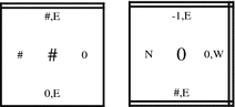
• 7. The following tile types fill in the last row of the transition block. Construct the following tile types:

  

5.3.3 Growing transition block tile types

The tile types that make up a growing transition block are all of the tile types in Sect. 5.3.2, in conjunction with the following tile types, which actually initiate the growth:

5.3.4 Tile types for single-bit modified counters

For all $x \in \{0,\ldots,c-2\},$ define the following (single-row modified counter) counting tile types.

5.3.5 Tile types for single-bit transition blocks

The following tile type is the last tile to attach in a single-row modified counter.

5.3.6 The first growing transition block

The following tile types initiate the growth of the first transition block.

5.3.7 The seed tile type

The following tile type is the seed tile type for our construction.

5.4 Construction of $T_{{\mathcal{F}}(X)}$

In this subsection, we construct the tile set $T_{{\mathcal{F}}(X)}.$ Recall that $(0,0) \in V\,\subsetneq\,\{0\ldots,c-1\} \times \{0,\ldots,c-1\}$ is the generator of X. For each $\vec{v} \in V,$ we construct the tile set

$$ T_{\vec{v}} = T_{\vec{v},\square} \cup T_{\vec{v},\uparrow} \cup T_{\vec{v},\rightarrow} \cup T_{\vec{v},\square,{\rm init}} \cup T_{\vec{v},\uparrow,{\rm init}} \cup T_{\vec{v},\rightarrow,{\rm init}} \cup T_{\vec{v},\ast} $$

Note that the tile sets $T_{\vec{v},\square}, T_{\vec{v},\uparrow},$ and $T_{\vec{v},\rightarrow}$ make up the bulk of the tile set $T_{\vec{v}}.$ The tile sets $T_{\vec{v},\square,{\rm init}}, T_{\vec{v},\uparrow,{\rm init}}, T_{\vec{v},\rightarrow,{\rm init}},$ and $T_{\vec{v},\ast}$ are used exclusively to self-assemble the initial stage and internal structure of ${\mathcal{F}}(X).$

We first define some standard operations on (sets of) tile types that we will ultimately apply to the tile types that we defined in Sects. 5.3.1, 5.3.2, 5.3.3, 5.3.4, 5.3.5, and 5.3.7.

Definition 5.11

Let t be a tile type, and T be a set of tile types.

• 1. The reflection of t about the line y = x, written as R _y=x(t), is the tile type t′ satisfying, for all $(x,y) \in U_2, t'(y,x) = t(x,y); R_{y=x}(T) = \left\{\left. R_{y=x}(t) \; \right| \; t \in T \right\}.$

• 2. The reflection of t about the y-axis, written as R _y-axis(t), is the tile type t′ satisfying, for all $\vec{u} \in \{(-1,0),(1,0)\}, t'(\vec{u}) = t(-\vec{u}); R_{y \hbox{-}{\rm axis}}(T) = \left\{\left. R_{y \hbox{-}{\rm axis}}(t) \; \right| \; t \in T \right\}.$

• 3. The reflection of t about the x-axis, written as R _x-axis(t), is the tile type t′ satisfying, for all $\vec{u} \in \{(0,-1),(0,1)\}, t'(\vec{u}) = t(-\vec{u}); R_{x \hbox{-}{\rm axis}}(T) = \left\{\left. R_{x \hbox{-}{\rm axis}}(t) \; \right| \; t \in T \right\}.$

Definition 5.12

Let t be a tile type, $U \subseteq U_2$ be a set of unit vectors, and $s \in \Sigma^*.$ The concatenation of s to the glue color on each side $\vec{u} \in U$ of t, written as C(t, U, s), is the tile type t′ satisfying, for all $\vec{u} \in U, t'(\vec{u}) = \left(\hbox{col}_t(\vec{u})\circ s,\hbox{str}_t(\vec{u})\right).$

We now have the tools that we need to construct the set $T_{\vec{v}}.$ When building the set $T_{\vec{v}},$ we consider the following cases.

• 1. $\vec{v} \in V - \{(0,0),(0,1),(1,0)\}.$ Let $\vec{u} = \vec{v}_{{\rm in}} - \vec{v}.$

  • (a) (hard-coded internal structure) If $\vec{v} \in (\{0\}\times \{0,\ldots,c-1\} \cup \{0,\ldots,c-1\} \times \{0\}),$ then let $T_{\vec{v},\ast} = \{t_{\vec{v},\ast} \},$ where, $t_{\vec{v},\ast}(\vec{u}) = \left(\vec{v},2\right),$ for all $\vec{u}' \in U_2 - \{\vec{u}\}$ such that $(\vec{v},\vec{v}+\vec{u}') \in E, t_{\vec{v},\ast}(\vec{u}') = \left(\vec{v}+\vec{u}',2\right),$ and, for all $\vec{u}' \in U_2-\{\vec{u}\}$ such that $(\vec{v},\vec{v}+\vec{u}') \not \in E, t_{\vec{v},\ast}(\vec{u}') = \left(\lambda,0\right).$

  • (b) (forward growth) We label this case as “forward growth” because the transition block of type “$\vec{v}\;$” will self-assemble before both counters of the same type. Furthermore, both counters will not grow toward from the x or y-axis.

    If $\vec{u} = (-1,0),$ then we construct $T_{\vec{v},\square}, T_{\vec{v},\uparrow},$ and $T_{\vec{v},\rightarrow}$ as follows.

    • i. Define the following sets of tile types.

      $$ \begin{aligned} T_{\S5.3.2} & = \left\{t \; \left| \; t\, \hbox{is a tile type defined in Sect.}\,5.3.2 \right. \right\} \cr T_{\S5.3.2,{\rm S}} & = \left\{t \; \left| t\, \in T_{\S5.3.2}\, \hbox{and the symbol `S' is in some glue color of}\, t\right. \right\}\cr T_{\S5.3.5} & = \left\{t \; \left| \; t\, \hbox{is a tile type defined in Sect.}\,5.3.5 \right. \right\} \end{aligned} $$

      Let

      $$ \begin{aligned} T_{\vec{v},\square} = & R_{y=x}(C\left(T_{\S5.3.2} - T_{\S5.3.2,{\rm S}},U_2,\vec{v}\right) \cup \cr & \quad C\left(C\left(T_{\S5.3.2,{\rm S}},\{(0,-1)\},\vec{v}_{{\rm in}}\right),U_2-\{(0,-1)\},\vec{v}\right)). \cr T_{\vec{v},\square,{\rm init}} = & R_{y=x}(C(C(T_{\S5.3.5},U_2-\{(0,-1)\},\vec{v}_{\rm in}),U_2-\{(0,-1)\},\vec{v})) \end{aligned} $$

      This ensures that the transition block of “type $\vec{v}\;$” binds to the horizontal counter of type “$\vec{v}_{\rm in}.$”

    • ii. Define the following sets of tile types.

      $$ \begin{aligned} T_{\S 5.3.1} & = \left\{t \; \left| \;t\,\hbox{is a tile type defined in Sect.}\,5.3.1 \right. \right\}\cr T_{\S 5.3.4} & = \left\{t \; \left| \; t\, \hbox{is a tiletypedefined in Sect.}\,5.3.4 \right. \right\} \cr T_{\S 5.3.1,{\rm Counting}} & = \left\{t \; \left| \; t\, \in T_{\S 5.3.1}\,\hbox{and}\, t\, \hbox{is defined in Group}\,1 \right.\right\}\cr T_{\S 5.3.1,{\rm Spacing}} & = T_{\S 5.3.1}-T_{\S 5.3.1,{\rm Counting}} \cr T_{\S 5.3.1,{\rm E}} & = \left\{t \;\left| t \in T_{\S 5.3.1}\, \hbox{and the symbol `E' is in some gluecolor of}\,t \right. \right\} \end{aligned} $$

      Let

      $$ \begin{aligned} T_{\vec{v},\uparrow} = & C\left( T_{\S5.3.1} - T_{\S5.3.1,{\rm E}},U_2,\vec{v}\right) \cup \cr &C\left(C\left(T_{\S5.3.1,{\rm Spacing}} \cap T_{\S5.3.1,{\rm E}},\{(1,0)\},(0,x)\right),U_2-\{(1,0)\},\vec{v}\right) \cup \cr & C\left(C\left(T_{\S5.3.1,{\rm Counting}} \cap T_{\S5.3.1,{\rm E}},\{(1,0)\},(1,x+1)\right),U_2-\{(1,0)\},\vec{v}\right)\cr T_{\vec{v},\uparrow,{\rm init}} = & C(C(T_{\S5.3.4},\{(1,0)\},(1,x)),U_2-\{(1,0)\},\vec{v}) \end{aligned} $$

    • iii. Let

      $$ \begin{aligned} T_{\vec{v},\rightarrow} = & R_{y=x}(C\left(T_{\S5.3.1} - T_{\S5.3.1,{\rm E}},U_2,\vec{v}\right) \cup\cr & C\left(C\left(T_{\S5.3.1,{\rm Spacing}} \cap T_{\S5.3.1,{\rm E}},\{(1,0)\},(x,0)\right),U_2-\{(1,0)\},\vec{v}\right) \cup \cr & C\left(C\left(T_{\S5.3.1,{\rm Counting}} \cap T_{\S5.3.1,{\rm E}},\{(1,0)\},(x+1,1)\right),U_2-\{(1,0)\},\vec{v}\right)) \cr T_{\vec{v},\rightarrow,{\rm init}} = & R_{y=x}(C(C(T_{\S5.3.4},\{(0,1)\},(x,1)),U_2-\{(0,1)\},\vec{v})) \end{aligned} $$

  • (c) (forward growth) If $\vec{u} = (0,-1),$ then we construct $T_{\vec{v},\square}, T_{\vec{v},\uparrow},$ and $T_{\vec{v},\rightarrow}$ as follows.

    • i. Let

      $$ \begin{aligned} T_{\vec{v},\square} = & C\left( T_{\S5.3.2} - T_{\S5.3.2,{\rm S}},U_2,\vec{v}\right) \cup \cr &C\left(C\left( T_{\S5.3.2,{\rm S}},\{(0,-1)\},\vec{v}_{\rm in}\right),U_2-\{(0,-1)\},\vec{v}\right) \cr T_{\vec{v},\square,{\rm init}} = & C(C(T_{\S5.3.5},U_2-\{(0,-1)\},\vec{v}_{\rm in}),U_2-\{(0,-1)\},\vec{v}) \end{aligned} $$

      This ensures that the transition block of “type $\vec{v}\;$” binds to the vertical counter of type “$\vec{v}_{\rm in}.$”

    • ii. Let $T_{\vec{v},\uparrow}, T_{\vec{v},\rightarrow}, T_{\vec{v},\uparrow,{\rm init}},$ and $T_{\vec{v},\rightarrow,{\rm init}}$ be defined as they were in case 2(a).

  • (d) (reverse growth) We label this case as “reverse growth” because one of the counters that we construct will grow toward the x or y-axis. Furthermore, the transition block of type “$\vec{v}\;$” will not self-assemble before both counters of the same type. We must take special care when constructing the tile types for a reverse growing counter (and transition block) because nice discrete self-similar fractals need not be symmetric. See Fig. 22 for an illustration of reverse growth.

    If $\vec{u} = (1,0),$ then we construct $T_{\vec{v},\square}, T_{\vec{v},\uparrow},$ and $T_{\vec{v},\rightarrow}$ as follows.

    • i. Define the following set of tile types.

      $$ \begin{aligned} T_{\S5.3.1,{\rm B}}& = \left\{t \; \left|t \in T_{\S5.3.1}\, \hbox{and the symbol `B' is in some glue color of}\, t\right.\right\}\cr T_{\S5.3.4,x=0} & = \left\{t \; \left| t \in T_{\S5.3.4} \, \hbox{and} \,x = 0\right.\right\} \end{aligned} $$

      Let

      $$ \begin{aligned} T_{\vec{v},\rightarrow} = & R_{y \hbox{-}{\rm axis}}(R_{y=x}(C\left(T_{\S5.3.1} - \left(T_{\S5.3.1,{\rm E}} \cup T_{\S5.3.1,{\rm B}}\right),U_2,\vec{v}\right) \cup \cr &C\left(C\left( T_{\S5.3.1,{\rm Spacing}} \cap T_{\S5.3.1,{\rm E}},\{(1,0)\},(c-x,0)\right),U_2-\{(1,0)\},\vec{v}\right) \cup \cr & C\left(C\left( T_{\S5.3.1,{\rm Counting}} \cap T_{\S5.3.1,{\rm E}},\{(1,0)\},(c-x+1,1)\right),U_2-\{(1,0)\},\vec{v}\right) \cup \cr & C\left(C\left( T_{\S5.3.1,{\rm B}},\{(0,-1)\},\vec{v}_{\rm in}\right),U_2-\{(0,-1)\},\vec{v}\right))) \cr T_{\vec{v},\rightarrow,{\rm init}} = & R_{y \hbox{-}{\rm axis}}(R_{y=x}(C(C(T_{\S5.3.4} - T_{\S5.3.4,x=0},\{(1,0)\},(x+1,0)),U_2 - \{(1,0)\},\vec{v}) \cup \cr & C(C(C(T_{\S5.3.4,x=0},\{(0,-1)\},\vec{v}_{\rm in}),\{(0,1)\},(c-x+1,0)), \cr & \quad\quad U_2-\{(0,-1),(1,0)\},\vec{v}))) \end{aligned} $$

    • ii. Let

      $$ \begin{aligned} T_{\vec{v},\square} = & R_{y\hbox{-}{\rm axis}}(R_{y=x}(C\left(T_{\S5.3.2},U_2,\vec{v}\right))) \cr T_{\vec{v},\square,{\rm init}} = & R_{y\hbox{-}{\rm axis}}(R_{y=x}(C\left(T_{\S5.3.5},U_2,\vec{v}\right))) \end{aligned} $$

      This ensures that the (reverse growing) transition block of “type $\vec{v}\;$” binds to the (reverse growing) horizontal counter of type “$\vec{v}.$”

    • iii. Let $T_{\vec{v},\uparrow}$ and $T_{\vec{v},\uparrow,{\rm init}}$ be defined as they were in case 2(a).

  • (e) (reverse growth) If $\vec{u} = (0,1),$ then we construct $T_{\vec{v},\square}, T_{\vec{v},\uparrow},$ and $T_{\vec{v},\rightarrow}$ as follows.

    • i. Let

      $$ \begin{aligned} T_{\vec{v},\uparrow} = & R_{x\hbox{-}{\rm axis}}(C\left( T_{\S5.3.1} - T_{\S5.3.1,{\rm E}},U_2,\vec{v}\right) \cup \cr & C\left(C\left( T_{\S5.3.1,{\rm Spacing}} \cap T_{\S5.3.1,{\rm E}},\{(1,0)\},(0,c-x)\right),U_2-\{(1,0)\},\vec{v}\right) \cup \cr & C\left(C\left( T_{\S5.3.1,{\rm Counting}} \cap T_{\S5.3.1,{\rm E}},\{(1,0)\},(1,c-x+1)\right),U_2-\{(1,0)\},\vec{v}\right)) \cr T_{\vec{v},\uparrow,{\rm init}} = & R_{x\hbox{-}{\rm axis}}(R_{y=x}(C(C(T_{\S5.3.4} - T_{\S5.3.4,x=0},\{(1,0)\},(0,x+1)),U_2 - \{(1,0)\},\vec{v}) \cup \cr & C(C(C(T_{\S5.3.4,x=0},\{(0,-1)\},\vec{v}_{\rm in}), \cr & \quad\quad \{(0,1)\},(0,c-x+1)),U_2-\{(0,-1),(1,0)\},\vec{v}))) \end{aligned} $$

      This ensures that the (reverse growing) vertical counter of “type $\vec{v}\;$” binds to the transition block of type “$\vec{v}.$”

    • ii. Let

      $$ \begin{aligned} T_{\vec{v},\square} = & R_{x\hbox{-}{\rm axis}}(C\left( T_{\S5.3.2},U_2,\vec{v}\right) \cr T_{\vec{v},\square,{\rm init}} = & R_{x\hbox{-}{\rm axis}}(C\left( T_{\S5.3.5},U_2,\vec{v}\right)) \end{aligned} $$

      This ensures that the (reverse growing) transition block of type “$\vec{v}\;$” binds to the (reverse growing) vertical counter of type “$\vec{v}.$”

    • iii. Let $T_{\vec{v},\rightarrow}$ and $T_{\vec{v},\rightarrow,{\rm init}}$ be defined as they were in case 2(a).

• 2. $\vec{v} \in \{(0,1),(1,0)\}.$ Let $\vec{u} = \vec{v}_{\rm in} - \vec{v}.$

  • (a) (forward growth) If $\vec{u} = (0,-1),$ then we construct $T_{\vec{v},\square}, T_{\vec{v},\uparrow},$ and $T_{\vec{v},\rightarrow}$ as follows.

    • i. Define the following sets of tile types.

      $$ \begin{aligned} T_{\S5.3.3} = & \left\{t \; \left| \; t\, \hbox{is a tile type defined in Sect.}\,5.3.3 \right. \right\} \cr T_{\S5.3.6} = & \left\{t \; \left| \; t\, \hbox{is a tile type defined in Sect.}\,5.3.6 \right. \right\} \end{aligned} $$

      Let

      $$ \begin{aligned} T_{\vec{v},\square} = & C\left( T_{\S5.3.2} - (T_{\S5.3.2,{\rm B}}),U_2,\vec{v}\right) \cup \cr & C\left(C\left( T_{\S5.3.2,{\rm B}} \cup T_{\S5.3.3},\{(0,-1)\},\vec{v}_{\rm in}\right),U_2-\{(0,-1)\},\vec{v}\right) \cr T_{\vec{v},\square,{\rm init}} = & C(T_{\S5.3.2} \cup T_{\S5.3.3},U_2,\vec{v}) \cup \cr & C\left(C\left(T_{\S5.3.6},\{(0,-1)\},(0,0)\right),U_2-\{(0,-1)\},\vec{v}\right) \end{aligned} $$

      This ensures that the growing transition block of “type $\vec{v}\;$” binds to the horizontal counter of type “$\vec{v}_{\rm in}.$”

    • ii. Let $T_{\vec{v},\uparrow}, T_{\vec{v},\rightarrow}, T_{\vec{v},\uparrow,{\rm init}},$ and $T_{\vec{v},\rightarrow,{\rm init}}$ be defined as they were in case 2(a).

  • (b) (forward growth) If $\vec{u} = (-1,0),$ then we construct $T_{\vec{v},\square}, T_{\vec{v},\uparrow},$ and $T_{\vec{v},\rightarrow}$ as follows.

    • i. Let

      $$ \begin{aligned} T_{\vec{v},\square} = & R_{y=x}(C\left( T_{\S5.3.2} - (T_{\S5.3.2,{\rm B}} \cup T_{\S5.3.3}),U_2,\vec{v}\right) \cup \cr & C\left(C\left( T_{\S5.3.2,{\rm B}} \cup T_{\S5.3.3},\{(0,-1)\},\vec{v}_{\rm in}\right),U_2-\{(0,-1)\},\vec{v}\right)) \cr T_{\vec{v},\square,{\rm init}} = & R_{y=x}(C(T_{\S5.3.2} \cup T_{\S5.3.3},U_2,\vec{v}) \cup \cr & C(C(T_{\S5.3.6},\{(0,-1)\},(0,0)),U_2-\{(0,-1)\},\vec{v})) \end{aligned} $$

      This ensures that the growing transition block of “type $\vec{v}\;$” binds to the horizontal counter of type “$\vec{v}_{\rm in}.$”

    • ii. Let $T_{\vec{v},\uparrow}, T_{\vec{v},\rightarrow}, T_{\vec{v},\uparrow,{\rm init}},$ and $T_{\vec{v},\rightarrow,{\rm init}}$ be defined as they were in case 2(a).

    Let T _seed be the singleton set containing the seed tile defined in Sect. 5.3.7, and let

    $$ T_{\vec{0}} = C\left(T_{\rm seed},\{(1,0),(0,1)\},(0,0)\right). $$

    Finally, we have

    $$ T_{{\mathcal{F}}(X)} = \bigcup_{\vec{v} \in V}{T_{\vec{v}}}, $$

Fig. 22

a depicts forward growth, b shows what happens if the tile set $T_{\vec{v},\rightarrow}$ were to simply “count in reverse,” and c is the desired result (that we achieve in our construction)

Figure 23 gives a visual interpretation of our construction. Our final TAS is ${\mathcal{T}}_{{\mathcal{F}}(X)} = \left(T_{{\mathcal{F}}(X)},\sigma,2\right),$ where σ consists of a single “seed” tile type placed at the origin. In general, if $X \,\subsetneq\, {\mathbb{N}}^2$ is a nice discrete self-similar fractal generated by V, then $\left| T_{{\mathcal{F}}(X)} \right| = O(|V|).$ Unfortunately, the hidden constant is rather large. For instance, our construction yields a tile set of 5983 tile types for the discrete self-similar fractal generated by the points in the left-most image in Fig. 23.

Fig. 23

Let V be the set of points in the left-most image. The first arrow represents our construction. The second arrow shows a magnified view of a particular point in V. Each point $\vec{0} \ne \vec{v} \in V$ can be viewed (in principle) as several sub-tile sets: $T_{\vec{v},\square}, T_{\vec{v},\rightarrow}, T_{\vec{v},\uparrow}, T_{\vec{v},\square,{\rm init}}, T_{\vec{v},\rightarrow,{\rm init}}, T_{\vec{v},\uparrow,{\rm init}},$ and $T_{\vec{v},\ast}$

5.5 Correctness of construction

It is routine to verify that our TAS ${\mathcal{T}}_{{\mathcal{F}}(X)} = (T_{{\mathcal{F}}(X)},\sigma_{{\mathcal{F}}(X)},2)$ is locally deterministic and self-assembles ${\mathcal{F}}(X)$ according to the recursion given in Definition 5.9.

6 Conclusion

The Tile Assembly Model is a powerful and robust model that abstracts laboratory-based DNA tile self-assembly. The model exhibits rich theoretical behavior in that it allows for the self-assembly of a computationally and geometrically diverse set of assemblies that form intricate shapes or perform (potentially Turing universal) computation. However, as our first two main results show, there are limitations to the kinds of shapes and patterns that can, even theoretically, self-assemble in the TAM.

In our first main (impossibility) result, we proved that non-trivial discrete self-similar fractals do not self-assemble (in either the strict or the weak sense) in any temperature 1 tile assembly system that is locally deterministic. The assumption of local determinism allows one to reason about the nature of self-assembly at temperature 1. From this, we derived that any shape or pattern that self-assembles in a locally deterministic temperature 1 tile assembly system is necessarily too simple to be a fractal. At the time of this writing, the question of whether or not the assumption of local determinism can be removed remains open.

In our second main theorem, also an impossibility result, we proved that certain kinds of “pinch-point” discrete self-similar fractals do not strictly self-assemble at any temperature. Unlike our first main theorem, the proof of our second main theorem exploits the underlying geometry of certain kinds of shapes in order to prove that they do not strictly self-assemble. This is a necessary feature of the proof because self-assembly at temperature 2 (or greater) can perform Turing universal comptuation. It remains to be seen whether or not our second main theorem can be extended to any non-trivial discrete self-similar fractal.

In our third (and final) main result, we exhibited a construction based on simple modified base-c counters that overcomes fundamental limitations of the TAM with respect to the self-assembly of discrete self-similar fractal structures. Our construction takes as input a simple description of a discrete self-similar fractal and produces a (possibly very large) tile assembly system in which an “approximation” (i.e., fibered version) of the input fractal strictly self-assembles. Other “shape approximation” techniques have been explored in the TAM by Kao and Schweller in (2008), and Soloveichik and Winfree in (2007). Note that both of the previous results are of the flavor, “if a lot of (possibly infinitely many) tile types are necessary for the self-assembly of some particular shape, then very few tiles types suffice for the self-assembly of another shape that closely resembles the original shape.” Our fiber construction applies to a class of (nice) discrete self-similar fractals. It not only preserves discrete fractal dimension but also produces fractal-like shapes that are visually similar to the input fractals. A natural extension of our third main theorem would be to show that every (connected) discrete self-similar fractal has a fibered version that strictly self-assembles. In other words, if $X \,\subsetneq\, {\mathbb{N}}^2$ is a connected discrete self-similar fractal, then is it always the case that X has a “fibered” version ${\mathcal{F}}(X)$ that strictly self-assembles? Of course, ${\mathcal{F}}(X)$ must also be similar to X in some reasonable sense.

For example, consider the ‘H’ fractal, whose generator is shown in Fig. 24. In Fig. 24, we sketch a naive application of our fiber construction to the H fractal. The result is some shape that is clearly not similar to the actual H fractal in any reasonable sense.

Fig. 24

a ‘H’ fractal generator; b Fibered ‘H’ fractal

The results in this paper continue to expand our knowledge about the boundaries of self-assembly in the Tile Assembly Model. We also present several open problems which, if answered, will significantly extend them. Such continued research should both benefit theoretical understanding of the model, as well as guiding the direction of laboratory based work.

References

Adleman LM, Cheng Q, Goel A, Huang M-D, Kempe D, de Espanés PM, Rothemund PWK (2002) Combinatorial optimization problems in self-assembly. In: Proceedings of the thirty-fourth annual ACM symposium on theory of computing, pp 23–32
Adleman LM, Kari J, Kari L, Reishus D (2002) On the decidability of self-assembly of infinite ribbons. In: Proceedings of the 43rd annual IEEE symposium on foundations of computer science, pp 530–537
Aggarwal G, Goldwasser MH, Kau M-Y, Schweller RT (2004) Complexities for generalized models of self-assembly. In: Proceedings of ACM-SIAM symposium on discrete algorithms
Doty D, Gu X, Lutz JH, Mayordomo E, Moser P (2005) Zeta-dimension. In: Proceedings of the thirtieth international symposium on mathematical foundations of computer science, Springer-Verlag, NY, pp 283–294
Graham RL, Knuth DE, Patashnik O (1994) Concrete mathematics. Addison-Wesley, Reading
Kao M-Y, Schweller RT (2007) Reducing tile complexity for self-assembly through temperature programming. In: Proceedings of the 17th annual ACM-SIAM symposium on discrete algorithms (SODA 2006), Miami, Florida, Jan 2006, pp 571–580
Kao M-Y, Schweller RT (2008) Randomized self-assembly for approximate shapes, International Colloqium on Automata, Languages, and Programming (ICALP) In: Aceto L, Damgård I, Goldberg LA, Halldórsson MM, Ingólfsdóttir A, Walukiewicz I (eds) Lecture notes in computer science, vol 5125. Springer, Berlin, pp 370–384
Kautz SM, Lathrop JI (2009) Self-assembly of the Sierpinski carpet and related fractals. In: Proceedings of the fifteenth international meeting on DNA computing and molecular programming, Fayetteville, Arkansas, USA, 8–11 June 2009 (to appear)
Lathrop JI, Lutz JH, Patitz Matthew J, Summers SM (2008) Computability and complexity in self-assembly. In: Proceedings of the fourth conference on computability in Europe Athens, Greece, 15–20 June 2008
Lathrop JI, Lutz JH, Summers SM (2009) Strict self-assembly of discrete Sierpinski triangles. Theor Comp Sci 410:384–405
Majumder U, LaBean TH, and Reif JH (2007) Activatable tiles for compact error-resilient directional assembly. In: Thirteenth international meeting on DNA computing (DNA 13), Memphis, Tennessee, 4–8 June 2007
Rothemund PWK (2001) Theory and experiments in algorithmic self-assembly. Ph.D. thesis, University of Southern California, December
Rothemund PWK, Winfree E (2000) The program-size complexity of self-assembled squares (extended abstract), STOC ’00. In: Proceedings of the thirty-second annual ACM symposium on theory of computing, New York, USA, ACM, pp 459–468
Seeman NC (1982) Nucleic-acid junctions and lattices. J Theor Biol 99:237–247
Soloveichik D, Winfree E (2007) Complexity of self-assembled shapes. SIAM J Comp 36(6):1544–1569
Wang H (1961) Proving theorems by pattern recognition—II. Bell Syst Tech J XL(1):1–41
Wang H (1963) Dominoes and the AEA case of the decision problem. In: Proceedings of the symposium on mathematical theory of automata, New York, 1962, Polytechnic Press of Polytechnic Institute of Brooklyn, Brooklyn, NY, pp 23–55
Winfree E (1998) Algorithmic self-assembly of DNA. Ph.D. thesis, California Institute of Technology, June
Acknowledgments
We thank David Doty, Jim Lathrop, Jack Lutz, and Aaron Sterling for useful discussions. We would especially like to thank an anonymous reviewer whose detailed comments have substantially improved the final version of this paper.
Author information
Authors and Affiliations
Corresponding author
Additional information
Preliminary version appeared in the Proceedings of The Fourteenth International Meeting on DNA Computing (DNA 14), Prague, Czech Republic, June 2–6, 2008. This author’s research was supported in part by NSF-IGERT Training Project in Computational Molecular Biology Grant number DGE-0504304.
Rights and permissions
About this article
Cite this article
Patitz, M.J., Summers, S.M. Self-assembly of discrete self-similar fractals. Nat Comput 9, 135–172 (2010). https://doi.org/10.1007/s11047-009-9147-7
Received:
Accepted:
Published:
Issue Date:
DOI: https://doi.org/10.1007/s11047-009-9147-7