
Abstract
Nowadays medical imaging plays a vital role in diagnosing the various types of diseases among patients across the healthcare system. Robust and accurate analysis of medical data is crucial to achieving a successful diagnosis from physicians. Traditional diagnostic methods are highly time-consuming and prone to handmade errors. Cost is reduced and performance is improved by adopting computer-aided diagnosis methods. Usually, the performance of traditional machine learning (ML) classification methods much depends on both feature extraction and selection methods that are sensitive to colors, shapes, and sizes, which conveys a complex solution when facing classification tasks in medical imaging. Currently, deep learning (DL) tools have become an alternative solution to overcome the drawbacks of traditional methods that make use of handmade features. In this paper, a new DL approach based on a hybrid deep convolutional neural network model is proposed for the automatic classification of several different types of medical images. Specifically, gradient vanishing and over-fitting issues have been properly addressed in the proposed model in order to improve its robustness by means of different tested techniques involving residual links, global average pooling layers, dropout layers, and data augmentation. Additionally, we employed the idea of parallel convolutional layers with the aim of achieving better feature representation by adopting different filter sizes on the same input and then concatenated as a result. The proposed model is trained and tested on the ICIAR 2018 dataset to classify hematoxylin and eosin-stained breast biopsy images into four categories: invasive carcinoma, in situ carcinoma, benign tumors, and normal tissue. As the experimental results show, our proposed method outperforms several of the state-of-the-art methods by achieving rate values of 93.2% and 89.8% for both image- and patch-wise image classification tasks, respectively. Moreover, we fine-tuned our model to classify foot images into two classes in order to test its robustness by considering normal and abnormal diabetic foot ulcer (DFU) image datasets. In this case, the model achieved an F1 score value of 94.80% on the public DFU dataset and 97.3% on the private DFU dataset. Lastly, transfer learning (TL) has been adopted to validate the proposed model with multiple classes with the aim of classifying six different wound types. This approach significantly improves the accuracy rate from a rate of 76.92% when trained from scratch to 87.94% when TL was considered. Our proposed model has proven its suitability and robustness by addressing several medical imaging tasks dealing with complex and challenging scenarios.
1 Introduction
Deep learning (DL) technology applied to medical imaging may become the most disruptive tool since the advent of digital imaging. Designing a DL model that can successfully classify multiple types of medical images is a challenging task today [37]. Robust and accurate classification of medical images is the first step towards a successful diagnosis that could save many people’s lives. However, medical imaging-classification tasks require an effective DL model to achieve high performance. Several issues need to be properly addressed when it comes to effective DL model design and training, such as gradient vanishing, over-fitting, model depth and width, lack of training data (due to the difficulty in collecting data and the need for an expert to label it), and imbalanced data.
The major aim of this paper is to present a robust DL model that addresses these issues and is able to improve the performance of various medical tasks. To validate the performance of the proposed model, three medical imaging classification tasks were used: (1) breast cancer—the automatic classification of hematoxylin and eosin (H&E)-stained breast biopsy images into four classes: invasive carcinoma, in situ carcinoma, benign tumors, and normal tissue; (2) diabetic foot ulcers (DFUs)—the automatic classification of foot skin images into two classes: normal (healthy) skin and abnormal skin DFU classes; and (3) wound types—the automatic classification of six types of wounds, including burns, hemangiomas, foot ulcers, leg ulcers, pressure ulcers, and toe ulcers. We chose these applications based on their characteristic differences. The main differences can be summarized as (1) different input sizes (224 × 224 and 512 × 512 pixels), (2) binary and multiple classes (two, four, and six) and (3) type of input images (red-green-blue images, histopathology).
The more relevant aspects that motivated us to choose these applications were the following: i) DL has been less employed in these medical imaging tasks; ii) achieving high performance is crucial to accurate diagnosis, but traditional machine learning (ML) methods in these applications have shown low performance; and iii) these tasks are challenging, which will help us to demonstrate the robustness of the proposed model. The rest of this section describes the target tasks, with the breast cancer scenario as the first.
The American Cancer Society recently reported that breast cancer is the most widespread cancer in the world [63]. According to DeSantis, approximately 40,000 breast cancer death cases, more than 60,000 in situ breast cancer cases and about 250,000 new cases of pervasive breast cancer were reported in 2017 [16]. Early diagnosis and treatment are required to enhance patients’ quality of life and to reduce morbidity rates. For example, histopathology is still essential to the diagnostic process because it distinguishes between pervasive and in situ carcinomas and between malignant and benign tissues [12]. Moreover, identification and diagnostic processes for various subtypes of breast cancer usually include tissue biopsy collection from identified masses using ultrasound imaging or mammography, followed by histological analysis. In general, after having been stained with H&E, tissue samples are visually assessed by pathologists via light microscopy. The complex nature of these tissues makes visual assessment of tissue microstructure and organization of the nucleus in the histological images highly subjective and time-consuming. Therefore, reducing the subjectivity of the disease classification process and enhancing diagnostic efficiency requires automated computer-aided diagnostic systems, which also reduces specialists’ workloads. Histology is the study of the microscopic structures of organic tissues. Histopathology deals with the histological structure of diseased tissues. In traditional histopathology, a pathologist visually examines tissue slides through a microscope, looking for specific structures and characteristics, such as cells, nuclei, etc. [10].
Early detection and diagnosis play an important role in effective patient care and treatment planning. To distinguish between malignant and benign lesions, breast tissue biopsies are used during cancer screening. Conversely, there are many variations in texture, heterogeneous structure, and appearance, which make the manual evaluation of sizeable histopathological images challenging [40]. This evaluation is laborious, time-consuming, and frequently dependent on one-sided human understanding. Therefore, evolving computer-aided diagnostic systems are the answer to the accurate classification of H&E-stained histological breast cancer images. Recently, DL outperformed up-to-date techniques in different areas of medical image analysis and ML, such as computer-based diagnosis [43], segmentation [36], detection [27], and classification [2]. In comparison with other types of learners, DL’s merit is its capability to achieve better or similar performance compared with humans. Feature extraction plays a crucial stage because the performance of the classifier is completely dependent on the attributes of the extracted high- and low-level features. In the medical field, DL has solved very challenging tasks and achieved high performance [18, 36]. The breast cancer task is the first to test the effectiveness of our model and to prove that it is able to achieve high performance in one of the most complex image types—H&E-stained breast biopsy images.
To validate the performance of the proposed model on images of different types and sizes, a DFU classification task was also considered. DFUs are open sores or wounds that form on the bottom of the foot. Early detection of DFUs can prevent amputation in many patients. To the best of our knowledge, there is a very limited number of DL models that are employed for DFU classification, namely DFUNet [24] and DFU_QUTNet [5]. Although these models achieve good results, the need to further improve the performance of DFU classification is important to help doctors make clinical decisions. Moreover, we trained and tested it on six different wound types in order to challenge our model. This wound classification task is very challenging due to the complex images. Other reasons to employ a wound-classification task were to test our model’s robustness with more than four classes of breast cancer tasks and to show the effect of adopting the same TL domain instead of a different one. The breast cancer, DFU, and wound classification tasks were challenging due to several issues:
-
A wide range of heterogeneous and complex image shapes, sizes, and colors.
-
Low contrast between target objects and backgrounds.
-
The high inter-class likeness between classes.
-
The requirement for an automatic and robust DL model to extract excellent features to enable distinction between classes.
-
Overlapped cells in the breast cancer task.
-
Patients’ ethnicities in the DFU and wound tasks.
The following outlines the main contribution of the research conducted in our experimental study:
-
A hybrid deep convolutional neural network (DCNN) model has been designed based on a combination of multi-branch parallel convolutional layers and residual links along with global average pooling. We employed the proposed model in three challenging medical-imaging tasks.
-
The proposed model was employed to classify H&E-stained breast-biopsy images into four classes. As the experiments revealed, we improved the accuracy performance of breast cancer classification tasks and outperformed previous methods of the state-of-the-art (SoTA). Our model achieved a classification rate of 93.2% when tackling unseen ICIAR 2018 images.
-
The proposed model was also employed to classify foot images into two classes. It achieved an F1-score value of 94.80% on the public DFU dataset.
-
Transfer learning (TL) from same domain was employed. The knowledge gained by our model’s learning from the first DFU dataset was transferred to improve the performance of the second DFU dataset, achieving a F1-score of 97.3%. Additionally, the model’s learning from both DFU datasets was transferred to classify six wound types, and this approach achieved an accuracy rate value of 87.94%. To the best of our knowledge, this is the first attempt to classify six types of wounds.
-
Testing on several challenging scenarios within the field of medical imaging has empirically demonstrated that our model is effective and robust.
-
As described, a concise review of the previous DL architectures and breast cancer classification methods was carried out.
-
Lastly, the image- and patch-wise classification models were adopted for this paper, as will be explained in forthcoming sections, when facing breast cancer tasks.
The rest of the paper is organized as follows: Section 2 reviews the related work, Section 3 explains the proposed methodology, Section 4 presents the results, and Section 5 draws conclusions.
2 Related work
In this section, we first review DL architectures, followed by the breast cancer classification task. We have not reviewed the DFU classification methods due to the limited number of research (only two articles: [5, 24]). Goyal et al. [24] employed a novel convolutional neural network (CNN) architecture named DFUNet to classify foot images into two classes, namely abnormal (DFU) and normal (healthy skin). In a similar manner, Alzubaidi et al. [5] proposed a novel CNN architecture for binary classification of foot images. Although both methods proposed a novel CNN architecture and achieved good results, the need for a better CNN architecture that produces excellent results is necessary.
2.1 Deep learning
DL is the cornerstone of current progress in the field of ML and is responsible for recent breakthroughs in several medical classification tasks, such as magnetic resonance imaging, heartbeats, and breast cancer. Recently, DL has become a major diagnostic element in several medical image tasks [31, 41] and has been effectively used to solve several challenging biomedical image-analysis tasks, such as breast ultrasound lesions [64], Parkinson’s disease [52], melanoma recognition [65], and sickle cell anemia [3].
Traditional ML methods require many steps to finalize the classification task—preprocessing, feature extraction, feature selection, training, and classification. These methods are sensitive to different sizes, complex shapes, and colors, and their effective performance relies on the selected features. However, DL has overcome the limitations of ML methods. It can simultaneously and automatically extract the features and achieve classification [38]. Although DL has greatly contributed to advancements in solving different medical imaging tasks [31, 41], the study and design of a better network model are crucial to improving performance [42].
Several DL architectures have been proposed in the last ten years [1, 32]. AlexNet was considered the first network to significantly improve CNNs [35]. Its major improvements were the introduction of the rectified linear unit (ReLU) activation function, a non-linear function that helps to prevent vanishing gradient issues, and the introduction of the idea of dropout as regularization. Dropout is a technique in which neurons are haphazardly activated to avoid over-fitting issues, thereby forcing data to obtain new pathways and giving the network the ability to generalize in a better way. Additionally, data augmentation was introduced, which means that when fed to the network, images are shown with random translation, rotation, and crop, forcing the network to be more aware of image attributes, rather than of the images themselves. Lastly, it stacked more convolutional layers before pooling layers, which improved classification accuracy.
Later, the VGGNet network was introduced [51]. Its major improvement, and the main difference, was the addition of more layers to improve accuracy. Following this, the GoogleNet network was introduced [55], in which the idea of using parallel convolutional layers with different filter sizes was employed. This idea showed great improvement in terms of feature extraction. The ResNet network developed the idea of residual links, in which every two layers concatenate with a short connection to help avoid gradient vanishing issues [26]. The DenseNet network proposed a more complex structure of entire blocks of layers connected to one another [28]. Several other networks were later designed, with their design ideas deriving from the main models mentioned above [54, 56, 57, 66].
These models trained and tested on a large ImageNet dataset consisting of natural images, such as pens, animals, and humans [49]. They were fine-tuned by transferring the ImageNet dataset learning to solve several computer vision and pattern recognition tasks [39, 45, 61]. The performance of these tasks has significantly improved because their features are similar to those of the ImageNet dataset. For example, applying TL to the ImageNet dataset for face, car, and object detection can enhance the performance of these tasks. However, the ImageNet dataset does not contain medical images; therefore, in medical imaging tasks, a model trained from scratch performs almost as well as standard ImageNet transferred models (such as GoogleNet, ResNet, etc.) [47].
Based on the study of the advantages of previous models, we designed our proposed model with more improvements. It combines the idea of parallel convolutions and residual connections as well as global average pooling and has proved to be very beneficial for gradient propagation because it has multipath propagation. The proposed structure enables the model to have better feature representation since it employs multi-branch parallel convolutional layers.
2.2 Breast cancer classification
In this section, we describe some of the SoTA breast cancer classification methods (binary and multi-class), which are classified as either traditional ML or DL methods. The objective of the nucleus morphology analysis is to discriminate between malignant and benign tissues. Based on this objective, numerous researchers use stained microscopy images to extract nuclei-based features in order to discriminate the tissues into two classes: malignant and benign (i.e., binary classification) [20, 21]. The circular Hough transform method was used by Filipczuk et al. [20] as an early detection process to select the nuclei candidates in the first step. The second step was the discrimination process between correct and incorrect nuclei candidates, using a support vector machine (SVM) technique. In [21], George et al. used a watershed technique to refine the nuclei contour and in [34], four clustering algorithms were tested for nuclei segmentation. Belsare et al. [11] utilized the spatial-color-texture segmentation technique for epithelial cells surrounding the lumen segmentation. They then extracted texture features to compare the linear discriminant analysis classifier performance and the SVM and k-Nearest Neighbors classifier performances.
Many researchers regard breast histology image classification as a multi-class problem, rather than as a binary problem (malignant or benign). Zhang [67] classified the images into three classes, namely invasive carcinoma, in situ carcinoma, and normal by using a mixture of two random subspace classifier collections—one is founded on multiple layer perceptrons, the other comprises SVM classifiers. Considering the feature extraction process, Zhang [67] combined the Curvelet transform with local binary pattern texture analysis. However, metastases detection in whole-image slides and histological image classifications are currently challenging tasks. In recent years, several studies have introduced automated approaches to address these challenges. For example, Kothari et al. [33] examined the classification of histological renal tumor images by employing organically decodable shape-based features in a multi-class classification model; the authors identified the tissue structure’s distribution in each image. Doyle et al. [17] introduced an automatic system for differentiation between high and low breast cancer grades from H&E-stained histology images. They used the features captured from a considerable number of images as well as spectral clustering to lower the feature-space dimensionality. Subsequently, the lowered feature set was used to train the SVM classifier to distinguish between high and low breast cancer grades and infected and non-infected cancer images. Wang et al. [62] proposed another framework based on the detection of cancer metastases in images of breast sentinel lymph nodes, using DL for classification of the whole slide.
More recently, the popularity of DL models has become widespread. Therefore, the authors take advantage of CNNs to classify breast histology images. The whole-slide images are employed by Cruz-Roa et al. [13] for invasive carcinoma detection based on the DL approach. This approach used a sizeable amount of tissue patches (each 100 × 100 pixels in size) for the CNN training. Because the extracted features enclose information about the tissue arrangement as well as the nuclei, the approach performs better than other up-to-date techniques. Spanhol et al. [53] developed a CNN model to categorize histopathological breast cancer images into two classes, malignant or benign. Araujo et al. [53] introduced a CNN model for the classification of H&E-stained breast histology images with an imperfect training-sample number. The classification process categorized the tissue condition into four classes: invasive carcinoma, in situ carcinoma, benign, and healthy. The features extracted via the CNN were employed to train classifiers of the SVM type. The achieved accuracy was 83.3% for carcinoma/non-carcinoma classification and 77.8% for four-class classification. In 2018, some researchers employed DL models to train on ICIAR 2018 breast histology image datasets to differentiate four different classes of histopathological breast cancer, namely normal, benign, in situ, and invasive carcinomas. Some researchers fine-tuned the pre-trained models and trained them on ICIAR 2018 datasets, while others designed their models for the task [6, 9, 19, 25, 30, 46, 50, 58].
Although all the above-mentioned approaches achieved good image-wise accuracies, the need for high-performance breast cancer diagnosis is indispensable. Furthermore, most of the CNNs employed in this research area were divided into shallow or deep networks. Shallow networks are sufficient for some applications; however, the multi-class breast cancer histology image classification task, which involves heterogeneous cells, complex shapes, noises, and colors, demands a network with a more complex graph structure and better feature extraction. Deep networks are those previously trained on nature images from the ImageNet dataset and then fine-tuned for breast cancer classification. However, their domain classifications differ, therefore, using the knowledge learned from the ImageNet nature images does not significantly improve performance. In medical imaging applications, a network trained from scratch could perform at the same level as networks pre-trained on the ImageNet dataset [4, 47].
3 Methodology
The next subsections detail the adopted methodology in this contribution and consist of the following:
-
Datasets.
-
Image-wise classification.
-
Patch augmentation of the training set.
-
Proposed model.
-
Training process.
3.1 Datasets
As previously stated, in this work we employed four different datasets differing in image type, number of classes, and shape. The first consists of H&E-stained breast biopsy images, the second and third refer to foot skin images, and the last corresponds to wound images. Next, we describe each one.
-
BACH 2018: the ICIAR 2018 Grand Challenge provided the dataset [8]. The uncompressed, high-resolution images (2040 × 1536 pixels) consisted of H&E-stained breast histology microscopy images, labeled as either normal tissue, benign lesion, in situ carcinoma, or invasive carcinoma, as shown in Fig. 1. The labeling stage was achieved by two medical steps, using identical acquisition cases, with an enlargement of 200. A total of 400 images were used (100 samples in each class) with a pixel scale of 0.42-mm–0.42-mm. These images were chosen so that the pathology recognition could be independently distinguished from the visible organization and the tissue structure. The dataset was divided into 300 images for the training set and 100 for the testing set. The original image was divided into 12 non-overlapping patches of 512 × 512 pixels in size. The label of each patch is inherited from the original image.
Fig. 1 
Samples of BACH 2018 dataset classes
-
DFU dataset (DFU 1): this dataset consisted of 1679 ft-image patches [24]. These patches were classified into two classes, normal and abnormal. The normal class had 641 images, while the abnormal class had 1038 images. The images were different sizes; therefore, to ensure a fair comparison, we resized all images to 224 × 224 pixels, which is similar to the input size of the SoTA approach on the same dataset. Furthermore, this size is halfway between the smallest and largest sizes, thus reducing deformation. Some samples of the dataset are shown in Fig. 2.
Fig. 2 
Samples of DFU 1 dataset classes. The first row shows the abnormal class; the second row shows the normal class
-
DFU dataset (DFU 2): this dataset consisted of 754 images of patients’ feet [5]. These images were manually labeled by an expert in the field as either normal or abnormal (DFU). The normal and abnormal patches were extracted from the images at a size of 224 × 224 pixels. The total number of patches was 1609, with 542 normal and 1067 abnormal (DFU). Previous research was conducted on this dataset by the authors of this article; therefore, the dataset was used even though it is a private dataset. A sample of the dataset is shown in Fig. 3.
Fig. 3 
Samples of DFU 2 dataset classes
-
Wound dataset: this dataset was a combination of Google search images and those of the Medetec dataset [23, 44]. Originally, thirteen types of images were collected for the wound-classification task. We then chose six classes out of the thirteen due to an imbalanced number of images. There were 71 burn images, 73 hemangioma images, 106 ft-ulcer images, 207 leg-ulcer images, 220 pressure-ulcer images, and 106 toe-ulcer images. To avoid this imbalance, we collected more images from a Google search for the burn, hemangioma, foot-ulcer, and toe-ulcer classes and also rotated some images from these classes at a 90-degree angle. As a result, they had approximately the same number of images as the leg- and pressure-ulcer classes. All images were resized to 224 × 224 pixels. Padding was used to avoid stretching or squashing the images. Lastly, all images were double-checked by an expert in the field to confirm the labels. Some samples of this dataset are shown in Fig. 4.
Fig. 4 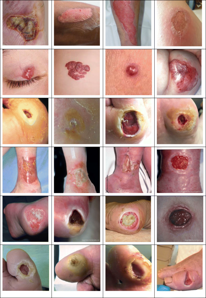
Samples of wound dataset classes. The first row shows the burn class, the second row shows the hemangioma class, the third row shows the foot-ulcer class, the fourth row shows the leg-ulcer class, the fifth row shows the pressure-ulcer class, and the sixth row shows the toe-ulcer class


3.2 Image-wise classification of breast cancer task
In this work, we considered the image classification process to be more suitably implemented in two stages. In the first stage, a patch-wise classifier was used to classify various patches, and in the second, the final image-wise classification was obtained by combining the classification results of image patches. Classification of breast cancer histology images into one of the four classes was based on the feature extraction correlated to the whole tissue organization as well as the extraction of the nuclei-correlated features. The information of the whole tissue structure was required for discrimination between invasive and in situ carcinomas. In contrast, the nuclei features—which involved information on a single nucleus-like shape or color in addition to the features of the nucleus organization, such as variability or density—helped discriminate between non-carcinoma and carcinoma. Therefore, the classification process relied on features varying in size from smaller than a nucleus to multiple nuclei wide.
The nuclei radius sizes ranged from approximately 1.26 to 4.62 m (3–11 pixels). Following the first observation, we assumed that the patch size of 224 × 224 pixels should be sufficient to cover the structures of the relevant tissue. Nevertheless, the whole images in the dataset were assigned labels of 2040 × 1536 pixels each, meaning that there was no guarantee that the small regions would contain related diagnostic information. This encouraged the use of larger image patches (512 × 512 pixels in size) to guarantee that an additional dependable label was maintained in the whole-image patches [7]. The classification process of one image is described in the following steps. Initially, the original image was partitioned into 12 non-overlapping patches of 512 × 512 pixels in size. The model was trained with these patches and the probabilities of patch classes were then calculated by the proposed trained model classifier. The second step included ensuring the accuracy of image-wise classification by using one of the following techniques related to patch probability fusion: i) sum of probabilities—the probabilities of each class patch are summed, then the class with the highest value is set for the test image; ii) maximum probability—the image label is decided by the patch with the highest class probability, and iii) majority voting—the most common patch label is selected to be the image label.
3.3 Patch augmentation of the training set
DL models are heavily determined by the training data volume. Higher complexity models demand more training images to perform well and prevent the problem of over-fitting. Lack of training data is the main problem in the medical field. In the case of breast histology images, the images had extremely large sizes, about 2040 × 1536 pixels each. To overcome the problems of lack of data and large image sizes, each image was partitioned into patches and augmented in a dataset using a set of robust transformations, which enriched and boosted the total number of images in the training set. Data augmentation techniques help to overcome the over-fitting issue. Then, we enhanced our proposal by applying different image processing techniques: i) rotation by angles of 45, 90, 135, 180, 225, 270, and 315 degrees, as illustrated in Fig. 5; ii) flipping in two directions—horizontal and vertical; iii) contrast and brightness of 51 and 81 degrees; iv) two-way zooming of the images—in and out; and v) color space by isolating a single color channel such as R, G, or B. In the breast cancer task, each training image was divided into 12 patches of 512 × 512 pixels, and each patch was duplicated 18 times using augmentation techniques. In the DFU task, we applied the same augmentation techniques and each patch was duplicated 18 times.

Augmentation process with rotation
3.4 The proposed model
To enhance the extraction of significant features for breast cancer classification and DFU tasks, we present the hybrid DCNN architecture. It combines the key aspects of the CNN structure, which include parallel convolutional layers and residual connections. The two main motivators for us to use this type of network were i) that adding more layers to a model to improve the performance is good up to a certain point, but this could lead to a drop in performance due to gradient diminishing issues, so we focused on increasing the width of the model, and ii) a shallow network with a simple structure of layers is suitable for some tasks. However, the breast cancer histology images and DFU classification tasks demand a network with a more complex graph architecture. The major aim of designing the proposed model was to provide the field with a robust model that is able to improve the performance of several SoTA methods when dealing with various medical tasks by means of addressing past issues and pitfalls related to crucial elements of DL, e.g., gradient vanishing, over-fitting, and feature extraction.
Specifically, gradient vanishing makes the network difficult to train because of the use of certain types of activation functions, such as sigmoid. These activation functions reduce the input size from large to small. Hence, big differences in the input will lead to small differences in the output. To address this problem, we employed the ReLU function, which does not reduce the input size. Residual connections and batch normalization layers were also employed in our model architecture to avoid problems. Residual links help to expedite the convergence of the network, helping to prevent gradient diminishing issues. Lastly, faster hardware was another solution, and we trained with GPU. Moreover, over-fitting occurs when the model learns a certain pattern from the training images and not from new data. We solved this problem by using image augmentation techniques. We also employed dropout and global average pooling layers (both explained later) to prevent this problem. Finally, parallel convolutional layers were applied for the extraction of good features to discriminate between classes. This included using four convolutional layers with four different filter sizes of 1 × 1, 3 × 3, 5 × 5, and 7 × 7. Each filter extracts different features, and by using different sizes, both small and large objects in the image can be detected. The proposed architecture is outlined as follows:
-
Generate several base networks, including shared parameters.
-
Optimize the information flow.
-
Enhance the training process of the deep network.
-
Allow the model to have an improved representation of features.
-
Improve the success rate of gradient propagation.
Our model’s architecture consists of a list of layers, as follows:
-
Input layer: this layer has three channels of 512 × 512 pixels. All input images were partitioned to 512 × 512 pixels then fed to our model for the patch-wise classification.
-
Convolutional layer (C): the main function of this layer is to extract the features by convolving the output of the prior layer with a group of learnable filters [59]. Three main parameters determine the output: depth (number of filters), zero-padding (adding zeros around the borders), and stride (number of pixels that the filter jumps). We employed 29 convolutional layers with different filter sizes (1 × 1, 3 × 3, 5 × 5, and 7 × 7).
-
Batch normalization layer (B): this layer was added after each convolutional layer. It normalizes every input channel via a mini-batch. It is used to expedite the training process of CNN models and diminish the sensitivity to network initialization [29]. It helps to avoid gradient vanishing problems.
-
Rectified linear unit (R): this function was added after each batch normalization layer. It filters data by using max (0, x) where x is the input to the neuron [15].
-
Global average pooling layer (G): this layer is employed to reduce the spatial dimensions from a three-dimensional tensor to a one-dimensional tensor. Average and maximum pooling layers use a sliding window (such as 2 × 2 or 3 × 3) to reduce the size. However, the global average pooling layer performs a more extreme kind of dimensionality reduction by turning the whole size into one dimension [14], as illustrated in Fig. 6. This layer is more robust to spatial translations and helps to avoid over-fitting.
Fig. 6 
Example of the average, maximum, and global average pooling layers

-
Fully connected layer (F): fully connected means that all the neurons of the first layer link to all the neurons of the second layer. The fully connected layer integrates the features to classify the breast cancer patches into four classes. Three fully connected layers were employed, and between them, dropout layers were inserted to avoid the problem of over-fitting.
Finally, on top of the fully connected layers, the softmax function was applied for classification in the softmax layer. This function was employed to map the non-normalized output of the model to a probability distribution of the predicted output classes. It is more robust to multi-class tasks than other activation functions. The total number of units in the softmax layer was equivalent to the number of classes that we aimed to classify. Thus, since we had four breast cancer classes, the softmax layer had four units. Figure 7 and Table 1 show the structure of the proposed model.

Proposed model architecture
3.5 Training process
The proposed model was trained and tested with four datasets. The training scenarios for each dataset are described next. The general training and testing pipeline are described in Fig. 8. For all datasets, the training process was achieved using stochastic gradient descent with momentum set to 0.9. The mini-batch size was 64 and MaxEpochs was 100, with a learning rate initially set to 0.001. We implemented our experiments with Matlab 2019 software and an Intel (R) processor Core TM i7-5829K CPU @ 3.30 GHz, 32 GB RAM, and 8 GB GPU.

Illustration of our training and testing pipeline
3.5.1 Breast Cancer training
The proposed model was first trained on the BACH 2018 Grand Challenge dataset with two different training scenarios implemented: scenario#1, using original images, and scenario#2, using original plus augmented images (see Section 3.3).
To verify and examine what the proposed model had learned, we fed it some images. The learnable kernels of the first six convolutional layers (C1, C2, C4, C5, C6) are shown in Figs. 9, 10, 11, 12, and 13, respectively.

Sample of a learnable kernel from the first convolutional layer (the color image is the original, and the gray-scale image is the filter)

Sample of a learnable kernel from the second convolutional layer (C2) (the color image is the original and the gray-scale image is the filter)

Samples of learnable kernels from the fourth convolutional layer (C4)

Samples of learnable kernels from the fifth convolutional layer (C5)

Samples of learnable kernels from the sixth convolutional layer (C6)
3.5.2 DFU 1 training
Next, we trained on the DFU 1 dataset. To prove that our model is robust, effective, and generic, we fine-tuned it to classify two classes of foot patches—normal and abnormal (DFU). The process for this task is explained as follows:
-
All images were resized to 224 × 224 × 3 pixels and we divided the data into 80% for training and 20% for testing.
-
All training images were augmented by the various techniques mentioned in Section 3.3. (patch augmentation of the training set).
-
The proposed model was fine-tuned by changing the input size and number of classes. We trained the model on original plus augmented images.
Figure 14 shows some learnable filters from our model’s first convolutional layer.

Samples of learnable kernels from the first convolutional layer trained on the DFU 1 dataset
3.5.3 DFU 2 training
Here, the training was conducted on the DFU 2 dataset. It was trained and tested on the DFU 2 dataset in three different scenarios: scenario#1 used all the images of the DFU 2 dataset for testing the proposed model trained on the DFU 1 dataset (trained on scenario#2); in scenario#2 our model was trained from scratch on the DFU 2 dataset plus augmented images. We divided the DFU 2 dataset into 80% for training and 20% for testing; and in scenario#3 we fine-tuning the proposed model that trained on the DFU 1 dataset then re-trained the model with the DFU 2 dataset. In this third case, we divided the DFU 2 dataset into 80% with augmented images for training purposes and the remaining 20% for testing.
3.5.4 Wound training
Finally, we trained and tested the wound dataset in the following two scenarios: in scenario#1 we trained our model from scratch on the wound dataset and divided the wound dataset into 80% for training and 20% for testing; in scenario#2, we first transferred the learning from the proposed model trained on the DFU 1 and DFU 2 datasets (the output-trained network from training on the DFU 2 dataset section in scenario#3 in 3.5.3 above) the model was fine-tuned for the task of wound classification. In this second scenario, the dataset was divided into 80% for training and the remaining 20% for testing.
TL is about leveraging the knowledge gained by training a DL model for a particular task and applying that knowledge to a different task. It simply works by training a base model on a base dataset and task, and then reusing the learned features, or transferring them, to a second target model to be trained on a target dataset and task. Currently, one of the biggest limitations of TL is the problem of negative transfer. When the base dataset is different from the target dataset, this is called negative transfer. Having a few images for TL in the same domain as the target dataset is better than having a large number of images in a different domain [4, 47]. In this work, the large dataset was the DFU data with augmented images, which was in the same domain as the target dataset, the wound dataset. Therefore, this type of TL significantly enhanced the wound classification performance, unlike using TL from natural images. The fine-tuning process is described in Fig. 15. The last fully connected layers were changed; Fig. 16 shows some learnable filters from the first convolutional layer of our model trained on wound classification.

Transfer learning pipeline

Samples of learnable kernels from the first convolutional layer trained on the wound dataset
4 Experimental results
This section describes the results obtained dealing with the breast cancer classification task and those of the DFU dataset.
4.1 Results of the breast cancer classification task
The proposed model’s accuracy was assessed. This evaluation process was implemented in two phases, patch-wise and image-wise, both for our model and for pre-trained models on unseen images.
-
Patch-wise classification results: we calculated the accuracy as illustrated in Eq. 1, where TP refers to true positives, TN refers to true negatives, FP refers to false positives, and FN refers to false negatives.
Patch-wise accuracies of the BACH 2018 dataset from our model and previous working methods are listed in Table 2. Our model, trained with the BACH 2018 dataset in scenario#1, achieved an accuracy of 84.7%. In scenario#2, the classification rate increased to 89.8% and outperformed previous SoTA methods.
-
Image-wise classification results: we used the three previously described evaluation techniques—the sum of probabilities, maximum probability, and majority voting—to measure the image-wise accuracy. The majority voting showed the highest results compared to other techniques; therefore, we considered these, as reported in Table 3. In the same scenarios as those used to evaluate the patch-wise results, data augmentation techniques helped improve the model’s accuracy from 85.9% when trained on original images (scenario#1) to 93.2% when trained on original plus augmented images (scenario#2).
Table 3 Comparative image-wise accuracy results on the BACH 2018 dataset from our model and the latest working methods
Our model surpassed the considered SoTA methods that used the majority voting technique on the BACH 2018 dataset. Most of these methods (e.g. GoogleNet and ResNet-101) dealing with small BACH 2018 datasets, are summarized in Table 3. These models are very deep, requiring more training images to perform well. Another issue is that these models were previously trained on natural images from the ImageNet dataset then fine-tuned for medical tasks, which are from a different domain. In medical imaging tasks, training a model from scratch is as good as using pre-trained models [4, 47].
4.2 Results of the DFU classification task (DFU 1 dataset)
We tested our model with the following evaluation metrics: recall (Eq. 2), precision (Eq. 3), and F1 score (Eq. 4). The results are reported in Table 4.
The total number of test images was 345. We obtained values for TP, FP, FN, and TN of 210, 11, 12, and 112, respectively. As reported in Table 4, our model achieved a higher precision, recall, and F1 score than DFUNet [24] by obtaining 95.1%, 94.5%, and 94.8%, respectively. However, DFUNet [24] achieved a precision of 94.5%, a recall of 93.4%, and an F1 score of 93.9%. To the best of our knowledge, DFUNet [24] is the SoTA network on the DFU 1 dataset. However, our model achieved results that were higher than DFUNet’s results. Furthermore, our model classified very challenging foot images, including wrinkled skin. Lastly, we have measured the testing time for the proposed model in this task. It needed 57 s to produce the results on test set images.
4.3 Results of the DFU classification task (DFU 2 dataset)
By transferring our model’s learning from the DFU 1 dataset and training it on the DFU 2 dataset, in scenario#3 our model achieved the highest precision, recall, and F1 score compared with other scenarios, obtaining 98.2%, 96.5%, and 97.3%, respectively. These results were calculated based on the values of TP, FP, FN, TN, which were 223, 4, 8, and 92, respectively. The total number of test images was 327. Additionally, the precision, recall, and F1 score for scenario#2 were 95.4%, 94.2%, and 94.7%, respectively. Lastly, although all images from the DFU 2 dataset were used for testing in scenario#1, the results were still competitive: precision of 88.2%, recall of 85.4%, and F1 score of 86.7%. The results of all scenarios are listed in Table 5. In scenario#3 our model outperformed the SoTA methods on the DFU 2 dataset [5], as reported in Table 6. Lastly, we have measured the testing time for the proposed model in this task. It needed 49 s to produce the results.
Our model’s results from the DFU 2 dataset prove that it is robust in the feature extraction and classification stages. It can handle various images for different medical imaging classification tasks and the advantage of adjusting to work on different tasks. Therefore, we employed it in the wound classification task to test its robustness.
4.4 Results of the wound classification task
There is a significant improvement in the results of scenario#1 and scenario#2 due to the TL technique, as reported in Table 7. Our model trained with scenario#1 achieved a precision of 77.4%, a recall of 73.9%, F1 score of 75.6%, and an accuracy of 76.92%. By transferring our model’s learning from the DFU 1 and DFU 2 datasets, our model trained with scenario#2 obtained a precision of 88.1%, a recall of 84.8%, an F1 score of 86.4%, and an accuracy of 87.94%.
Lastly, we have measured the testing time for the proposed model in this task. It needed 76 s to produce the results. The wound classification task was very challenging due to noisy, complex, and different color images; however, the proposed model overcame these challenges and proved that it is robust in different tasks. The achieved results in all tasks are used by doctors as a “second opinion” to aid definitive decision-making.
5 Conclusions
We proposed a hybrid deep CNN model as a tool for the automatic and robust classification of complex images within the field of medical imaging. The addressed classification tasks are challenging due to the different sizes, complex shapes, various colors, and variety of image types. The proposed model for classification combined several ideas, including parallel convolutional layers, residual connection, and global average pooling layer. The architecture of the proposed model has been proven to address three well-known pitfalls of DL, including gradient vanishing, over-fitting, and providing an improved representation of features. We first trained our model on the original images of the BACH 2018 Grand Challenge dataset (ICIAR 2018) to classify H&E-stained breast biopsy images into four classes: invasive carcinoma, in situ carcinoma, benign tumor, and normal tissue. To handle the small number of BACH 2018 images for training, in this study we applied several data augmentation techniques to the original images. These enhancements improved the performance of our method and achieved a classification rate of 93.2% and 89.8% for image-wise and patch-wise classification, respectively.
Specifically, the proposed method outperformed SoTA methods when dealing with the BACH 2018 dataset. Moreover, our method was trained and tested on two different DFU datasets in order to classify two classes of foot skin—normal and abnormal. The experimental results reported it achieved outstanding results when compared to SoTA networks tackling the DFU classification task. Additionally, our proposal achieved an F1 score of 94.8% on the first addressed DFU dataset and a value of 97.3% on the second addressed DFU dataset. To further test its effectiveness, the proposed model was used to classify six classes of wounds, and it achieved an outstanding performance of 87.94%. Moreover, we believe the methods proposed in this work can be used as a pre-trained model to classify images in the same domain. We plan to adopt the proposed model for other medical imaging tasks as future work.
References
Alzubaidi L, Zhang J, Humaidi AJ, Al-Dujaili A, Duan Y, Al-Shamma O, Santamaría J, Fadhel MA, Al-Amidie M, Farhan L (2021) Review of deep learning: concepts, CNN architectures, challenges, applications, future directions. J Big Data 8(1):1–74
Alzubaidi L, Al-Shamma O, Fadhel MA, Farhan L, Zhang J, Duan Y (2020) Optimizing the performance of breast Cancer classification by employing the same domain transfer learning from hybrid deep convolutional neural network model. Electronics 9(3):445
Alzubaidi L, Fadhel MA, Al-Shamma O, Zhang J, Duan Y (2020) Deep learning models for classification of red blood cells in microscopy images to aid in sickle cell Anemia diagnosis. Electronics 9(3):427
Alzubaidi L, Fadhel MA, Al-Shamma O, Zhang J, Santamaría J, Duan Y, Oleiwi SR (2020) Towards a better understanding of transfer learning for medical imaging: a case study. Appl Sci 10(13):4523
Alzubaidi L, Fadhel MA, Oleiwi SR, al-Shamma O, Zhang J (2020) DFU_QUTNet: diabetic foot ulcer classification using novel deep convolutional neural network. Multimed Tools Appl 79:15655–15677. https://doi.org/10.1007/s11042-019-07820-w
Alzubaidi L, Hasan RI, Awad FH, Fadhel MA, Alshamma O, Zhang J (2019) Multi-class breast Cancer classification by a novel two-branch deep convolutional neural network architecture. In proceedings of the 12th international conference on developments in eSystems engineering (DeSE), pp. 268–273
Araújo T, Aresta G, Castro E, Rouco J, Aguiar P, Eloy C, Polónia A, Campilho A (2017) Classification of breast cancer histology images using convolutional neural networks. PLoS One 12(6):e0177544
Aresta G, Araújo T, Kwok S, Chennamsetty SS, Safwan M, Alex V, … Fernandez G (2019) Bach: grand challenge on breast cancer histology images. Med Image Anal 56:122–139
Awan R; Koohbanani NA; Shaban M; Lisowska A; Rajpoot N (2018) Context-aware learning using transferable features for classification of breast cancer histology images. In proceedings of the international conference on image analysis and recognition, springer, Cham, June 2018; pp. 788–795
Barker J, Hoogi A, Depeursinge A, Rubin DL (2016) Automated classification of brain tumor type in whole-slide digital pathology images using local representative tiles. Med Image Anal 30:60–71
Belsare A, Mushrif M, Pangarkar M, Meshram N (2015) Classification of breast cancer histopathology images using texture feature analysis. In proceedings of the 10th TENCON conference. Macao, China
Bi WL, Hosny A, Schabath MB, Giger ML, Birkbak NJ, Mehrtash A, Allison T, Arnaout O, Abbosh C, Dunn IF, Mak RH (2019) Artificial intelligence in cancer imaging: clinical challenges and applications. CA Cancer J Clin 69(2):127–157
Cruz-Roa A, Basavanhally A, Gonzalez F, Gilmore H, Feldman M, Ganesan S, Shih N, Tomaszewski J, Madabhushi A (2014) Automatic detection of invasive ductal carcinoma in whole slide images with convolutional neural networks. In proceedings of SPIE medical imaging conference. San Diego, California, USA
Cui Y, Zhou F, Wang J, Liu X, Lin Y, Belongie S (2017) Kernel pooling for convolutional neural networks. In proceedings of the IEEE conference on computer vision and pattern recognition. Honolulu
Dahl GE, Sainath TN, Hinton GE (2013) Improving deep neural networks for LVCSR using rectified linear units and dropout. In proceedings of the international conference on acoustics, Speech and Signal Processing, Vancouver
DeSantis CE, Ma J, Goding Sauer A, Newman LA, Jemal A (2017) Breast cancer statistics, 2017, racial disparity in mortality by state. CA Cancer J Clin 67(6):439–448
Doyle S, Agner S, Madabhushi A, Feldman M, Tomaszewski J (2008) Automated grading of breast cancer histopathology using spectral clustering with textural and architectural image features. In proceedings of the international symposium on biomedical imaging: from Nano to macro. Paris, France
Esteva A, Robicquet A, Ramsundar B, Kuleshov V, DePristo M, Chou K, Cui C, Corrado G, Thrun S, Dean J (2019) A guide to deep learning in healthcare. Nat Med 25(1):24–29
Ferreira CA, Melo T, Sousa P, Meyer MI, Shakibapour E, Costa P, Campilho A (2018) Classification of breast cancer histology images through transfer learning using a pre-trained inception ResNet v2. In proceedings of the international conference on image analysis and recognition. Springer, Cham, pp 763–770
Filipczuk P, Fevens T, Krzyżak A, Monczak R (2013) Computer-aided breast cancer diagnosis based on the analysis of cytological images of fine needle biopsies. IEEE Trans Med Imaging 32(12):2169–2178
George YM, Zayed HH, Roushdy MI, Elbagoury BM (2013) Remote computer-aided breast cancer detection and diagnosis system based on cytological images. IEEE Syst J 8(3):949–964
Golatkar A, Anand D, Sethi A (2018) Classification of breast cancer histology using deep learning. In International Conference Image Analysis and Recognition. Springer: Cham, Switzerland, pp 837–844
Google-images-medetec-combined:https://github.com/mlaradji/deep-learning-for-wound-care/tree/master/data/google-images-medetec-combined (n.d.) (accessed on 7 April 2020)
Goyal M, Reeves ND, Davison AK, Rajbhandari S, Spragg J, Yap MH (2018) DFUNet: Convolutional neural networks for diabetic foot ulcer classification. IEEE Trans Emerg Topics Comput Intell:1–12
Guo Y, Dong H, Song F, Zhu C, Liu J (2018) Breast Cancer histology image classification based on deep neural networks. In: Proceedings of the International Conference Image Analysis and Recognition. Springer, Cham, Switzerland, pp 827–836
He K, Zhang X, Ren S, Sun J (2016) Deep residual learning for image recognition. In: Proceedings of the IEEE Conference on Computer Vision and Pattern Recognition, Las Vegas, NV, USA, pp 770–778
Herent P, Schmauch B, Jehanno P, Dehaene O, Saillard C, Balleyguier C, Arfi-Rouche J, Jégou S (2019) Detection and characterization of MRI breast lesions using deep learning. Diagn Interv Imaging 100(4):219–225
Huang G, Liu Z, Van Der Maaten L, Weinberger KQ (2017) Densely connected convolutional networks. In: Proceedings of the IEEE conference on computer vision and pattern recognition. Honolulu, HI, USA, pp 4700–4708
Ioffe S, Szegedy C (2015) Batch normalization: Accelerating deep network training by reducing internal covariate shift. In: International Conference on Machine Learning. PMLR, pp 448–456
Kassani SH, Kassani PH, Wesolowski MJ, Schneider KA, Deters R (2019) Breast cancer diagnosis with transfer learning and global pooling. In: 2019 International Conference on Information and Communication Technology Convergence (ICTC). IEEE, Jeju, Korea (South), pp 519–524
Ker J, Wang L, Rao J, Lim T (2017) Deep learning applications in medical image analysis. IEEE Access 6:9375–9389
Khan A, Sohail A, Zahoora U, Qureshi AS (2019) A survey of the recent architectures of deep convolutional neural networks. Artif Intell Rev, 1–62
Kothari S, Phan JH, Young AN, Wang MD (2013) Histological image classification using biologically interpretable shape-based features. BMC Med Imaging 13(1):9
Kowal M, Filipczuk P, Obuchowicz A, Korbicz J, Monczak R (2013) Computer-aided diagnosis of breast cancer based on fine needle biopsy microscopic images. Comput Biol Med 43(10):1563–1572
Krizhevsky A, Sutskever I, Hinton GE (2012) Imagenet classification with deep convolutional neural networks. In Advances in Neural Information Processing Systems, pp 1097–1105.
Lateef F, Ruichek Y (2019) Survey on semantic segmentation using deep learning techniques. Neurocomputing 338:321–348
Lu L, Wang X, Carneiro G, Yang L (2019) Deep learning and convolutional neural networks for medical imaging and clinical informatics. Springer, Berlin/Heidelberg, Germany, p 201
LeCun Y, Bengio Y, Hinton G (2015) Deep learning. Nature 521(7553):436–444
Li Y, Huang C, Ding L, Li Z, Pan Y, Gao X (2019) Deep learning in bioinformatics: introduction, application, and perspective in the big data era. Methods 166:4–21
Li C, Wang X, Liu W, Latecki LJ, Wang B, Huang J (2019) Weakly supervised mitosis detection in breast histopathology images using concentric loss. Med Image Anal 53:165–178
Litjens G, Kooi T, Bejnordi BE, Setio AAA, Ciompi F, Ghafoorian M, van der Laak JAWM, van Ginneken B, Sánchez CI (2017) A survey on deep learning in medical image analysis. Med Image Anal 42:60–68
Lv E, Wang X, Cheng Y, Yu Q (2019) Deep ensemble network based on multi-path fusion. Artif Intell Rev 52(1):151–168
Maier A, Syben C, Lasser T, Riess C (2019) A gentle introduction to deep learning in medical image processing. Z Med Phys 29(2):86–101
Medetec Wound Database (2020) http://www.medetec.co.uk/files/medetec-image-databases.html. Accessed 7 April
Mohanty SP, Hughes DP, Salathé M (2016) Using deep learning for image-based plant disease detection. Front Plant Sci 7:1419
Nawaz W, Ahmed S, Tahir A, Khan HA (2018) Classification of breast cancer histology images using AlexNet. In: Proceedings of the International Conference on Image Analysis and Recognition. Springer, Cham, Switzerland, pp 869–876
Raghu M, Zhang C, Kleinberg J, Bengio S (2019) Transfusion: understanding transfer learning for medical imaging. In: Advances in Neural Information Processing Systems, pp 3347–3357
Roy K, Banik D, Bhattacharjee D, Nasipuri M (2019) Patch-based system for classification of breast histology images using deep learning. Comput Med Imaging Graph 71:90–103
Russakovsky O, Deng J, Su H, Krause J, Satheesh S, Ma S, Huang Z, Karpathy A, Khosla A, Bernstein M, Berg AC (2015) Imagenet large scale visual recognition challenge. Int J Comput Vis 115(3):211–252
Sarker MI, Kim H, Tarasov D, Akhmetzanov D (2019) Inception architecture and residual connections in classification of breast Cancer histology images. arXiv 2019, arXiv:1912.04619. Available online https://arxiv.org/abs/1912.04619. Accessed on 28 December 2019
Simonyan K, Zisserman A (2014) Very deep convolutional networks for large-scale image recognition. arXiv preprint arXiv:1409.1556
Sivaranjini S, Sujatha CM (2019) Deep learning based diagnosis of Parkinson’s disease using convolutional neural network. Multimedia tools and applications, 1-13
Spanhol FA, Oliveira LS, Petitjean C, Heutte L (2016) Breast cancer histopathological image classification using convolutional neural networks. In: Proceedings of the 2016 International Joint Conference on Neural Networks (IJCNN), Vancouver, BC, Canada, pp 2560–2567
Szegedy C, Ioffe S, Vanhoucke V, Alemi A (2017) Inception-v4 inception-ResNet and the impact of residual connections on learning. In: Proceedings of the 31th AAAI Conference on Artificial Intelligence, vol 31, no 1
Szegedy C, Liu W, Jia Y, Sermanet P, Reed S, Anguelov D, ..., Rabinovich A (2015) Going deeper with convolutions. In Proceedings of the IEEE Conference on Computer Vision and Pattern Recognition, pp. 1–9
Szegedy C, Vanhoucke V, Ioffe S, Shlens J, Wojna Z (2016) Rethinking the inception architecture for computer vision. In: Proceedings of the IEEE Conference on Computer Vision and Pattern Recognition, pp 2818–2826
Targ S; Almeida D; Lyman K (2016) ResNet in ResNet: generalizing residual architectures, arXiv 2016, arXiv:1603.08029. Available online: https://arxiv.org/abs/1603.08029 (accessed on 2 January 2020)
Vang YS, Chen Z, Xie X (2018) Deep learning framework for multi-class breast cancer histology image classification. In proceedings of the international conference image analysis and recognition. Springer, Cham, pp 914–922
Vedaldi A, Lenc K (2015) Matconvnet: convolutional neural networks for MATLAB. In proceedings of the 23rd ACM international conference on multimedia. Brisbane
Wang Z, Dong N, Dai W, Rosario SD, Xing EP (2018) Classification of breast cancer histopathological images using convolutional neural networks with hierarchical loss and global pooling. In proceedings of the international conference on image analysis and recognition. Springer, Cham, pp 745–753
Wang F, Jiang M, Qian C, Yang S, Li C, Zhang H, Wang X, Tang X (2017) Residual attention network for image classification. In: Proceedings of the IEEE Conference on Computer Vision and Pattern Recognition, pp 3156–3164
Wang D, Khosla A, Gargeya R, Irshad H, Beck AH (2016) Deep learning for identifying metastatic breast cancer. Cornell University Library, New York (NY)
Ward EM, DeSantis CE, Lin CC, Kramer JL, Jemal A, Kohler B, Brawley OW, Gansler T (2015) Cancer statistics: breast cancer in situ. CA Cancer J Clin 65(6):481–495
Yap MH, Goyal M, Osman F, Ahmad E, Marti R, Denton E, Juette A, Zwiggelaar R (2018) End-to-end breast ultrasound lesions recognition with a deep learning approach. In: Medical imaging 2018: Biomedical applications in molecular, structural, and functional imaging, vol 10578. International Society for Optics and Photonics, p 1057819
Yu Z, Jiang X, Zhou F, Qin J, Ni D, Chen S, … Wang T (2018) Melanoma recognition in dermoscopy images via aggregated deep convolutional features. IEEE Trans Biomed Eng 66(4):1006–1016
Zagoruyko S; Komodakis N (2016) Wide residual networks, arXiv 2016, arXiv:1605.07146. Available online: https://arxiv.org/abs/1605.07146 (accessed on 2 January 2020)
Zhang B (2011) Breast cancer diagnosis from biopsy images by serial fusion of random subspace ensembles. In proceedings of the 4th international conference on biomedical engineering and informatics (BMEI2011). Shanghai, China
Acknowledgments
We would like to express our gratitude to Dr.Sameer R. Oleiwi from Nursing College, Muthanna University, for his effort in confirming the labels of wound images. We would also like to thank the Queensland University of Technology for supporting us.
Author information
Authors and Affiliations
Corresponding author
Ethics declarations
Ethical approval
This article does not contain any studies with human participants or animals performed by any of the authors.
Conflict of interest
The authors declare that they have no conflict of interest.
Additional information
Publisher’s note
Springer Nature remains neutral with regard to jurisdictional claims in published maps and institutional affiliations.
Rights and permissions
About this article

Cite this article
Alzubaidi, L., Fadhel, M.A., Al-Shamma, O. et al. Robust application of new deep learning tools: an experimental study in medical imaging. Multimed Tools Appl 81, 13289–13317 (2022). https://doi.org/10.1007/s11042-021-10942-9
Received:
Revised:
Accepted:
Published:
Issue Date:
DOI: https://doi.org/10.1007/s11042-021-10942-9