Image watermarking in real oriented wavelet transform domain

Abstract

In this paper, we propose blind and non-blind watermarking schemes in the real oriented wavelet transform (ROWT) domain. The ROWT, which is a member of the dual tree complex wavelet transform (DTCWT) family, is chosen as a watermarking domain since the DTCWT has recently emerged as an important new image processing tool. Existing watermarking schemes based on the DTCWT usually lack high embedding capacity. This is mainly due to the fact that the left inverse and the right inverse of the DTCWT (including the ROWT) are not equal. We have observed a relation when the ROWT follows its left inverse, and have used this relation to develop two watermarking schemes in the ROWT domain. Experimental results show that the proposed ROWT based watermarking schemes not only have a much higher capacity than the existing DTCWT based watermarking schemes, but are also robust to various image modification operations such as cropping, Gaussian filter, Gaussian noise, and salt and pepper noise.

1 Introduction

Digital watermarking is an effective tool in multimedia that provides solution for digital rights such as broadcast monitoring, piracy, owner identification, copy right protection, proof of ownership, media authentication, fingerprinting/transaction tracking, copy control, legacy enhancement etc. [1, 2, 5, 7, 12, 16, 21, 35, 41]. Recently, digital watermarking has been also used to enhance security of biometric systems [13, 23].

The main idea in digital watermarking is that a watermark (which may be a binary image, a gray scale image, a signature etc.) is embedded into a multimedia (which may be an image, a video, an audio etc.) to obtain a watermarked media. The watermarked media is made available in public domain. To solve digital right claims associated with a watermarked media available in public domain, a watermark is extracted/detected from the watermarked media and the extracted watermark is compared with all possible embedded watermarks using a comparator function to identify an embedded watermark. A comparator function consists of two main components- a similarity measure function and a threshold value. Similarity measure function returns similarity value between two watermarks. If a similarity value is greater than the threshold then watermarks are matched, otherwise not. Maximization of accurate identification rate (which directly depends on the capacity/size/length of watermark) is a common goal in all watermarking applications. If very intelligent adversary with an aim to defeat a watermarking system is present in public domain, then watermarking problems are very challenging.

A watermarked media available in public domain may be attacked by adversary or innocent/common multimedia processing operations. Robust watermarking are designed such that after any kind of attack on the watermarked media, the watermark is successfully identified. Such watermarking schemes are applicable for copyright protection, owner identification etc. Fragile watermarking are designed such that if watermarked media is attacked then watermark is not identified. Such watermarking schemes are helpful in tamper detection. Semi-fragile watermarking schemes are robust against adversary attack and fragile against innocent/common multimedia processing operations [5].

Depending on the required information of original data (original media/cover work and original watermark) in watermark extractor, watermarking schemes are divided into three categories, namely blind (oblivious or public), non-blind (non-oblivious or private) and semi-blind watermarking schemes [1]. Watermarking schemes that do not require the information of original data in their watermark extractor are called blind watermarking schemes. Non-blind watermarking schemes require complete information of original data in their watermark extractor while, semi-blind watermarking schemes need a part of information of original data in their watermark extractor. Usually, non-blind watermarking scheme are more robust than blind watermarking schemes. Non-blind watermarking schemes are applicable in those scenarios, where automated search of original media is possible [19]. However, blind watermarking schemes are more attractive, since, in many watermarking applications, original media can not be made available at watermark extractor [1, 10, 20, 27].

According to domain in which watermark is embedded, watermarking schemes are classified into two broad categories: spatial-domain and transformed-domain schemes. In spatial domain watermarking schemes [13], [11] the watermark is embedded by directly modifying the pixel values of an original media. The main idea in transformed-domain watermarking schemes is that an original media is transformed, transformed coefficients of the original media are modified and the inverse transform is applied on the updated transformed coefficients to obtain the watermarked media. Some popular transformed domain for digital watermarking are discrete cosine transform (DCT) [28], discrete wavelet transform (DWT) [19], discrete Fourier transform (DFT) [38], singular value decomposition (SVD) [2], Fractional transform [3] etc. A proper domain should be selected for watermarking according to application scenarios, for instance, DCT based watermarking schemes have better performance for JPEG [40] standard images and DWT domain based watermarking schemes have better performance for JPEG 2000 [36] standard images [37]. Therefore, scopes exist to develop improved watermarking schemes in various transform domain.

Recently, transforms of complex wavelet family have emerged as very important multimedia processing tools. Complex wavelet integrates the phase concept of Fourier transform and multi-resolution analysis concept of wavelets. DTCWT (dual-tree-complex-wavelet-transform) is an important member of complex wavelet transforms family. An extended version of DTCWT for images is called ROWT (real-oriented-wavelet-transform) [33]. The details of complex wavelets and ROWT are discussed in Section 2. Applications of complex wavelet transforms family have been found in estimating image geometrical structures, local displacement and motion estimation [24, 31, 33], denoising [44], image segmentation [34], seismic imaging [26], disparity estimation [17] and content based image retrieval [8, 14, 15]. In watermarking field, researchers have developed various watermarking schemes in a domain of complex wavelet transform (CWT) family [4, 22, 39, 43]. However, small watermark length/size is a major limitation in all the existing CWT family based watermarking schemes. A main reason for this limitation may be that the left inverse and the right inverse of family members of CWT are not equal.

In this paper, a relation has been found when the ROWT follows its left inverse. Based on this relation, two watermarking schemes have been developed in the ROWT domain for images. One is the non-blind watermarking scheme and other is the blind watermarking scheme. Exploring the observed relation in the proposed non-blind watermarking scheme was easy. However, doing so in the proposed blind watermarking scheme was proved to be difficult. This challenge has been solved by a deep investigation of the Quotient-Remainder theorem for the real numbers. The proposed watermarking schemes have been compared with the existing CWT family based watermarking schemes and a drastic increase in the length/size of watermarks has been shown in both the proposed watermarking schemes. In the experiments, meaningful binary logo watermarks have been used in the proposed watermarking schemes. The performance of the proposed watermarking schemes have been studied under various common image processing operations such as cropping, Gaussian filtering, Gaussian noise and salt and pepper noise. Experimental results demonstrate that the proposed watermarking schemes are more robust than the existing CWT family based watermarking schemes.

The rest of the paper is organized as follows. In Section 2, the ROWT, its implementation on an image and its observed property are discussed.

The proposed watermarking schemes are described in Section 3. Experiments results are analyzed in Section 4. Conclusions are provided in Section 5.

2 The ROWT and its observed property

In this section, ROWT and its implementation on gray scale image are discussed followed by the observed property of the ROWT. A list of main symbols used in this section is defined in Table 1.

Table 1 List of symbols used in Section 2

2.1 The ROWT

Selesnick et al. [33] defined the complex wavelet function and the complex scaling function as follows:

$$\begin{array}{@{}rcl@{}} \psi_{c}(t) &=& \psi_{h}(t) + \mathrm{j}\psi_{g}(t) \end{array} $$

(1)

$$\begin{array}{@{}rcl@{}} \phi_{c}(t) &=& \phi_{h}(t) + \mathrm{j}\phi_{g}(t) \end{array} $$

(2)

where, ψ _c (t) is an analytic function, i.e. $\psi _{g}(t)=\mathcal {H}[\psi _{h}(t)]$, $\mathcal {H}[.]$ is the Hilbert transform operator, ϕ _h is the scaling function corresponding to the wavelet ψ _h , ϕ _g is the scaling function corresponding to the wavelet ψ _g and j is the square root of -1.

The ROWT consists of six real-oriented 2D wavelets that are defined as follows,

$$\begin{array}{@{}rcl@{}} \psi_{l}(x,y)& = &\frac{1}{\sqrt{2}}(\psi_{1,l}(x,y)+\psi_{2,l}(x,y)), \end{array} $$

(3)

$$\begin{array}{@{}rcl@{}} \psi_{l+3}(x,y)&=&\frac{1}{\sqrt{2}}(\psi_{1,l}(x,y)-\psi_{2,l}(x,y)), \end{array} $$

(4)

where l=1,2,3,

$$\psi_{1,1}(x,y)=\phi_{h}(x)\psi_{h}(y), \quad \psi_{2,1}(x,y)=\phi_{g}(x)\psi_{g}(y),$$

$$\psi_{1,2}(x,y)=\psi_{h}(x)\phi_{h}(y), \quad \psi_{2,2}(x,y)=\psi_{g}(x)\phi_{g}(y),$$

$$\psi_{1,3}(x,y)=\psi_{h}(x)\psi_{h}(y), \quad \psi_{2,3}(x,y)=\psi_{g}(x)\psi_{g}(y),$$

and two scaling functions that are defined as follows,

$$\phi_{1}(x,y)=\phi_{h}(x)\phi_{h}(y), \quad \phi_{2}(x,y)=\phi_{g}(x)\phi_{g}(y).$$

The factor $1/\sqrt 2$ in (3)–(4) is the normalization factor that is used to make the sum/difference operation an orthonormal operation. The ROWT have been implemented on an image using two fast-wavelet-transforms (FWT) [9, 25, 33] in parallel. The analysis filter bank (Fig. 1) of the ROWT is used to decompose an image into eight sub-bands and synthesis filter bank (Fig. 2) of the ROWT is used to reconstruct back the image from its decomposed sub-bands. The details of the one-level forward ROWT and the one-level inverse ROWT are discussed in the algorithm 1 and the algorithm 2 respectively.

Table 2

Table 3

Fig. 1

Analysis filter bank for decomposition of image/signal [32, 33]. a Real scaling analysis filter h ₀ corresponding to ϕ _h . b Imaginary scaling analysis filter g ₀ corresponding to ϕ _g . c Real wavelet analysis filter h ₁ corresponding to ψ _h . d Imaginary wavelet analysis filter g ₁ corresponding to ψ _g

Fig. 2

Synthesis filter bank for reconstruction of image/signal [32, 33]. a Real scaling synthesis filter $\tilde {h}_{0}$ corresponding to ϕ _h . b Imaginary scaling synthesis filter $\tilde {g}_{0}$ corresponding to ϕ _g . c Real wavelet synthesis filter $\tilde {h}_{1}$ corresponding to ψ _h . d Imaginary wavelet synthesis filter $\tilde {g}_{1}$ corresponding to ψ _g

One-level implementation of the ROWT [32, 33] on a sample gray scale image is shown in Fig. 3. The size of the sample image is 256×256 pixels and size of the each decomposed sub-band is 128×128 pixels. Note that the sub-bands A ₁ and A ₂ are called approximation sub-bands, the sub-bands P _V , P _H and P _D are called positive sub-bands, and the sub-bands N _V , N _H and N _D are called negative sub-bands.

Fig. 3

The ROWT of an image (a). a: a sample image, b: sub-band A ₁ corresponding to ϕ ₁, c: sub-band A ₂ corresponding to ϕ ₂, d: sub-band P _V corresponding to ψ ₁, e: sub-band N _V corresponding to ψ ₄, f: sub-band P _H corresponding to ψ ₂, g: sub-band N _H corresponding to ψ ₅, h: sub-band P _D corresponding to ψ ₃ i: sub-band N _D corresponding to ψ ₆

2.2 Observed property of the ROWT

Let A ₁ and A ₂ be the approximation sub-bands and P _𝜃 s and N _𝜃 s be the positive and negative sub-bands respectively obtained from an image I on applying the ROWT [32, 33] on it , where 𝜃=H,V and D. Modify P _𝜃 s and N _𝜃 s as follows:

$$\begin{array}{@{}rcl@{}} P_{\theta}^{\prime} &=& P_{\theta}+Q_{1}, \end{array} $$

(5)

$$\begin{array}{@{}rcl@{}} N_{\theta}^{\prime} &=& N_{\theta}+Q_{2}, \end{array} $$

(6)

where, Q ₁ and Q ₂ are two real matrices that have a size equal to the size of the P _𝜃 s and N _𝜃 s. Let $I^{\prime }$ be the image reconstructed by applying the inverse ROWT on A ₁, A ₂, $P_{\theta }^{\prime }$s and $N_{\theta }^{\prime }$s sub-bands. Let $P_{\theta }^{\prime \prime }$s and $N_{\theta }^{\prime \prime }$s be the positive and negative sub-bands respectively obtained from $I^{\prime }$ by applying the ROWT on it. Then the following two relations have been observed:

$$\begin{array}{@{}rcl@{}} P_{\theta}^{\prime\prime}+N_{\theta}^{\prime\prime} = P_{\theta}+N_{\theta}+ Q_{1} \text{if} \ Q_{2}=Q_{1}, \end{array} $$

(7)

$$\begin{array}{@{}rcl@{}} P_{\theta}^{\prime\prime}-N_{\theta}^{\prime\prime} = P_{\theta}-N_{\theta}+Q_{1} \text{if} \ Q_{2}=-Q_{1}. \end{array} $$

(8)

A numerical example is provided in Fig. 4 to elaborate and verify the observed property of the ROWT. Figure 4 reports a small mismatch in the observed property. This small mismatch may be due to the truncation error in data representation and transform implementation. Note that inverse ROWT followed by ROWT does not make an identity transform. This situation is very different than the DCT, DWT and other transforms, wherein, inverse of a transform followed by itself makes an identity transform. This main difference between the ROWT and other transforms emphasizes the need for significant changes to the conventional watermarking models. In this paper, the observed property of the ROWT is used as a building block in the proposed watermarking schemes.

Fig. 4

Illustration of the observed property of the ROWT using numerical examples

3 Watermarking schemes

This section is divided into two subsections: non-blind watermarking schemes (Section 3.1) and blind watermarking schemes (Section 3.2). In Section 3.1, a traditional non-blind watermarking scheme, proposed non-blind watermarking scheme in the ROWT domain and watermark estimation rules from extracted watermark bits are discussed. In Section 3.2, a traditional blind watermarking scheme and proposed blind watermarking scheme in the ROWT domain are discussed. A list of symbols used in Section 3 is explained in Table 2.

Table 2 List of symbols used in Section 3

3.1 Non-blind watermarking schemes

A watermark embedding algorithm and corresponding watermark extraction algorithm of a traditional non-blind watermarking scheme are explained in algorithm 7 and algorithm 8 respectively. A numerical example is provided in Fig. 5 to illustrate the traditional non-blind watermarking scheme.

Fig. 5

A numerical example to illustrate a traditional non-blind watermarking algorithms. a Embedding algorithm. b: Extraction algorithm

Figure 6a and b summarize the components of the proposed non-blind watermark embedding and watermark extraction algorithms. The details of the watermark embedding and watermark extraction algorithms are discussed in algorithm 9 and algorithm 10. In the algorithm 9, watermark bits are embedded by utilizing (5) and (6), and in the algorithm 10, watermark bits are extracted by utilizing (7)/(8). A numerical example is provided in Fig. 7 to illustrate the proposed non-blind watermarking scheme.

Fig. 6

Overview of proposed non-blind watermarking algorithm

Fig. 7

A numerical example to illustrate the proposed non-blind watermarking scheme in the ROWT domain. In this example, α=3, and G(P)=G(N)=1

According to the traditional non-blind watermarking scheme (Algorithms 7 and 8), one watermark bit is embedded at one position and one watermark bit is extracted using one position. According to the proposed non-blind watermarking scheme (Algorithms 9 and 10), one watermark bit is embedded at two positions and one watermark bit is extracted using two positions. This is the main difference between the traditional non-blind watermarking scheme and the proposed non-blind watermarking scheme.

A watermark is estimated from the extracted watermark bits. In watermark estimation, the following three scenarios can arise:

• 1. A watermark is embedded once and each watermark bit is embedded once. In this case, π is an one-to-one function and one watermark W _e is estimated as follows:

  $$\begin{array}{@{}rcl@{}} W_{e}(l_{2})=W(l_{1}). \end{array} $$

  (9)

  Table 5

  Table 6

• 2. A watermark is embedded n (>1) times and each watermark bit is embedded n times. In this scenario, π is a many-to-one function, the redundancy of the watermark is n, and n watermarks ${{W_{e}^{i}}}$ are estimated as follows:

  $$\begin{array}{@{}rcl@{}} {{W_{e}^{i}}}(l_{2})=W(\pi^{-1}(\pi(l_{1}))_{i}), \end{array} $$

  (10)

  where, i=1,2,⋯n, π ⁻¹ is the inverse map of π and

  $$\pi^{-1}(\pi(l_{1}))=\{\pi^{-1}(\pi(l_{1}))_{i}\}. $$

• 3. A watermark is embedded once and each watermark bit is embedded n (an odd number) times. In this situation, π is a many-to-one function, the redundancy of the watermark bits is n and one watermark is estimated by the voting method as follows:

  $$\begin{array}{@{}rcl@{}} W_{e}(l_{2})=b(\pi^{-1}(\pi(l_{1}))), \end{array} $$

  (11)

  where,

  $$\begin{array}{@{}rcl@{}} b(.)&=& \left\{ \begin{array}{ccc} 0 & \text{if} & c_{0}(.)>c_{1}(.) \\ 1 & \text{if} & c_{0}(.)<c_{1}(.) \end{array} \right., \end{array} $$

  (12)

  and c ₀(π ⁻¹(π(l ₁))) and c ₁(π ⁻¹(π(l ₁))) are a number of 0 watermark bits and 1 watermark bits, respectively, at the π ⁻¹(π(l ₁)).

Table 7

Table 8

3.2 Blind watermarking schemes

3.2.1 A traditional blind watermarking scheme

A watermark embedding algorithm and corresponding watermark extraction algorithm of a traditional blind watermarking scheme are explained in Algorithms 3 and 4 respectively. The core idea in the watermark embedding algorithm is that if watermark bit is one, then make the watermarking coefficient odd multiple of watermarking strength else if watermark bit is zero, then make the watermarking coefficient even multiple of watermarking strength. The core idea in the watermark extraction algorithm is that if watermarked coefficient is odd multiple of watermarking strength, then extracted watermark bit is one else if watermarked coefficient is even multiple of watermarking strength, then extracted watermark bit is zero. A numerical example is provided in Fig. 8 to illustrate the traditional blind watermarking scheme.

Fig. 8

A numerical example to illustrate a traditional blind watermarking algorithms. a Embedding algorithm. b: Extraction algorithm

Table 9

3.2.2 Special mathematical properties

The core theory in the traditional blind watermarking scheme is to make the watermarked coefficients an even/odd multiple of watermarking strength. Success of this theory depends on the fact that watermarked coefficients are well preserved after applying a transform succeeded by its inverse transform. This fact is not true for the ROWT. The core theory in the proposed blind watermarking scheme in the ROWT domain is to add/subtract a value in coefficients of positive and negative sub-bands of the original image according to the observed property of the ROWT such that remainder of sum of the added value and sum/difference of the coefficients of the positive and negative sub-bands belongs to a well defined desired interval. Success of this theory is guaranteed by the relations (7) and (8). The added values are found using specially derived mathematical properties based on the Quotient-Remainder theorem. The added/subtracted values depend on watermarking strength and a desired interval.

Table 10

Let μ be a non-negative real number and α be a positive real number. Then the remainder r can be found such that μ=α m+r, where m is the non-negative integer and 0≤r<α. This is the Quotient-Remainder theorem. Here, m is termed as the quotient. Based on the Quotient-Remainder theorem, the following properties hold:

• 1. remainder (r ₁) of $\mu +\frac {\alpha -r}{2}$ is $\frac {\alpha }{2}+\frac {\delta \alpha }{2}<r_{1}<\alpha -\frac {\delta \alpha }{2}$, if δ α<r<α−δ α,

• 2. remainder (r ₂) of $\mu +\frac {\alpha +\delta \alpha }{2}$ is $\frac {\alpha }{2}+\frac {\delta \alpha }{2}\leq r_{2}\leq \frac {\alpha }{2}+\frac {3\delta \alpha }{2}$, if r≤δ α,

• 3. remainder (r ₃) of $\mu +\frac {2\alpha -\delta \alpha }{2}$ is $\frac {\alpha }{2}-\frac {3\delta \alpha }{2}\leq r_{3}<\alpha -\frac {\delta \alpha }{2}$, if r≥α−δ α,

• 4. remainder (r ₄) of $\mu +\frac {2\alpha -r}{2}$ is $\frac {\delta \alpha }{2}<r_{4}<\frac {\alpha }{2}-\frac {\delta \alpha }{2}$, if δ α<r<α−δ α,

• 5. remainder (r ₅) of $\mu +\frac {2\alpha +\delta \alpha }{2}$ is $\frac {\delta \alpha }{2}\leq r_{5} \leq \frac {3\delta \alpha }{2}$, if r≤δ α,

• 6. remainder (r ₆) of $\mu +\frac {3\alpha -\delta \alpha }{2}$ is $\frac {\alpha }{2}-\frac {3\delta \alpha }{2}\leq r_{6}<\frac {\alpha }{2}-\frac {\delta \alpha }{2}$, if r≥α−δ α,

as long as $\delta \in \left (0,\frac {1}{3} \right )$. Moreover,

• 7. $\frac {\alpha }{2}+\frac {\delta \alpha }{2}\leq r_{1},r_{2},r_{3}<\alpha -\frac {\delta \alpha }{2}$,

• 8. $\frac {\delta \alpha }{2}\leq r_{4},r_{5},r_{6}<\frac {\alpha }{2}-\frac {\delta \alpha }{2}$.

In properties 1–6, the term μ is equivalent to the sum (or difference) of coefficients of the positive and negative sub-bands of an original image in the ROWT domain. Properties 1–6 are used in the proposed blind watermark embedding Algorithm 5 and properties 7–8 are used in the proposed blind watermark extraction Algorithm 6.

3.2.3 The proposed blind watermarking scheme in the ROWT domain

Figure 9a summarizes the components in the watermark embedding algorithm and Fig. 9b summarizes the components in the watermark extraction algorithm. The details of the watermark embedding algorithm and watermark extraction algorithms are discussed in Algorithms 5 and 6 respectively. A numerical example is provided in Fig. 10 to illustrate the proposed blind watermarking scheme.

Fig. 9

Overview of proposed blind watermarking algorithm

Fig. 10

A numerical example to illustrate the proposed blind watermarking technique in the ROWT domain. In this example, α=5, δ=0.25, G(P)=G(N)=1 and k=1

Like the proposed non-blind watermarking scheme, in this scheme also (Algorithms 5 and 6), one watermark bit is embedded at two positions and one watermark bit is extracted using two positions.

4 Experiments, results, and analysis

We have performed six experiments for a detailed analysis of the proposed watermarking schemes. Experiment 1 tests the proposed watermarking schemes and studies the effect of embedding strength and error controller. This experiment helps to find optimal embedding strength and error controller. Experiment 2 elaborates the importance of the observed property of ROWT. Experiment 3 studies the performance of the proposed watermarking schemes and studies the effect of embedding strength and error controller under the formatting operation on the watermarked images. Experiment 4 evaluates the performance of the proposed watermarking schemes under various attacks on formatted watermarked images. Experiment 5 compares the proposed watermarking schemes and existing watermarking schemes without any post operations/attacks on the watermarked images. Experiment 6 compares the performance of the proposed watermarking schemes and existing watermarking schemes under various post operations/attacks on the watermarked images.

Table 11

Table 12

In the experiments, we have used a data-set that consists of six host images and five watermarks. Figure 11a shows all host images (h ₁, h ₂, h ₃, h ₄, h ₅, h ₆) and Fig. 11b shows all watermarks (W ₁, W ₂, W ₃, W ₄ and W ₅) of the data-set. Each host image is an eight bit gray scale image of size 256×256 pixels and each watermark is a black and white (binary) image of size 128×128 pixels. We have used all the combinations of the host images and the watermarks to obtain different watermarked images.

Fig. 11

Data-set

A common setup in all the experiments is as follows. We have repeated a watermark three times by embedding it once in V, H and D sub-bands of a host image. This makes watermarks of an effective size of 3×128×128 pixels. L ₁ consists of all the locations of V, H, D sub-bands of a host image. π is a simple left-right-top-bottom scan map. We have set G(P)=G(N)=1. For the proposed blind watermarking scheme, we have used k=1.

4.1 Experiment1: testing of proposed watermarking schemes and effect of embedding strength and error controller

• Non-blind watermarking scheme.  We have implemented the proposed non-blind watermarking scheme on the data-set (shown in Fig. 11) for various embedding strengths (α= 1:1:20). Peak-signal-to-noise-ratio (PSNR) [30] measures the visual similarity between the original image and the watermarked image, and normalized-Hamming-similarity (NHS) [30] measures the similarity between the embedded watermark and corresponding extracted watermarks. The NHS ranges from zero to one ([0,1]). If NHS is 1, then both watermarks are the same. If NHS is 0, then watermarks are negative of each other. If NHS=0.5, then watermarks are uncorrelated and have no common information. We have observed that the embedding strength decreases PSNR and does not affect NHS. Figure 12a shows a sample watermarked image which corresponds to host image h ₄, original watermark W ₁, and embedding strength of 3 and ensures no visual degradation in the watermarked image. The obtained watermarked images are 64-bit (double format) gray scale images of size 256×256 pixels. Figure 12b, c, and d show watermarks extracted from V, H and D sub-bands, respectively, of a watermarked image (Fig. 12a) and ensure very good quality of extracted watermarks. We have obtained very close results for all other combinations of host images and original watermarks of the data-set (Fig. 11).

  Fig. 12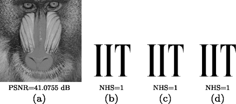

  

  A sample result of non-blind watermarking scheme at embedding strength of 3. a: A sample watermarked image. b: Watermark extracted from V sub-bands of (a). c: Watermark extracted from H sub-bands of (a). d: Watermark extracted from D sub-bands of (a)

• Blind watermarking scheme.  We have also implemented the proposed blind watermarking scheme on the same data-set for various embedding strengths (α=1:1:20) and various error controllers (δ=0.00,0.05,0.10,0.15,0.20,0.25,0.30,0.33). We have observed that the embedding strength and error controller decrease PSNR and do not affect NHS. Figure 13a shows a sample watermarked image which corresponds to host image h ₄, original watermark W ₁, embedding strength of 5 and error controller δ of 0.25 and ensures no visual degradation in the watermarked image. Like the non-blind watermarking scheme, the obtained watermarked images are 64-bit (double format) gray scale images of size 256×256 pixels. Figure 13b, c, d show watermarks extracted from V, H and D sub-bands, respectively, of a watermarked image (Fig. 13a) and ensure very good quality of extracted watermarks. We have obtained very close results for all other combinations of host images and original watermarks of the data-set (Fig. 11).

  Fig. 13

  

  A sample result of blind watermarking scheme at embedding strength of 5 and error controller of 0.25. a: A sample watermarked image. b: Watermark extracted from V sub-bands of (a). c: Watermark extracted from H sub-bands of (a). d: Watermark extracted from D sub-bands of (a)

4.2 Experiment 2: what if the observed property of the ROWT is not utilized?

This experiment implements the ROWT based traditional non-blind and blind watermarking schemes which do not utilize the observed property of the ROWT. For this traditional non-blind watermarking scheme, the fundamental embedding and extraction rules are according to Algorithms 3 and 4, respectively, and for this traditional blind watermarking scheme, the fundamental embedding and extraction rules are according to Algorithms 7 and 8, respectively. If we do not incorporate the observed property of the ROWT, then the length of a watermark can be doubled as a watermark can be embedded and extracted from each of the six detailed sub-bands of an image.

• Non-blind watermarking scheme.  Fig. 14 shows a sample result of a traditional non-blind watermarking scheme in the ROWT domain which does not use the observed property of the ROWT. We have observed that watermarks extracted from positive sub-bands are very close to embedded watermark and watermarks extracted from negative sub-bands are not matched with embedded watermark. Therefore, only positive sub-bands can be used for watermarking. The slightly better quality of extracted watermarks (see Fig. 12b, c, d and Fig. 14b, c, d) affirms that the proposed non-blind watermarking scheme with the observed ROWT property has slightly better performance than the ROWT based traditional non-blind watermarking scheme.

  Fig. 14

  

  A traditional non-blind watermarking scheme in the ROWT domain without the observed property. a: A sample watermarked image. b: Watermark extracted from positive V sub-band of (a). c: Watermark extracted from positive H sub-band of (a). d: Watermark extracted from positive D sub-band of (a). e: Watermark extracted from negative V sub-band of (a). f: Watermark extracted from negative H sub-band of (a). g: Watermark extracted from negative D sub-band of (a).

• Blind watermarking scheme.  Fig. 15 shows a sample result of a traditional blind watermarking scheme in the ROWT domain which does not utilize the observed ROWT property. We have observed that extracted watermarks are very noisy (Fig. 15). Figures 13 and 15 ensure that proper utilization of the observed ROWT property has significantly improved the quality of extracted watermarks.

  Fig. 15

  

  A traditional non-blind watermarking scheme in the ROWT domain without the observed property. a: A sample watermarked image. b: Watermark extracted from positive V sub-band of (a). c: Watermark extracted from positive H sub-band of (a). d: Watermark extracted from positive D sub-band of (a). e: Watermark extracted from negative V sub-band of (a). f: Watermark extracted from negative H sub-band of (a). g: Watermark extracted from negative D sub-band of (a)

4.3 Experiment 3: the effect of embedding strength and error controller on formatted watermarked images

In Experiment1, host images are eight bit gray scale images and watermarked images are 64-bit (double format) gray scale images. In most of the watermarking applications, the same format of host images and watermarked images is a common request. We have applied the uint8 operation on all the watermarked images to obtain formatted watermarked images (eight bit gray scale images).

• Non-blind watermarking scheme.  Figure 16a shows the PSNR curve of the sample formatted watermarked images and Fig. 16b shows the NHS curves of the watermarks extracted from the V, H and D sub-bands of the sample formatted watermarked images. The sample formatted watermarked images corresponds to the combination of host image h ₄ and watermark W ₁. Figure 16a depicts a decrease in the PSNR with embedding strength. Moreover, the PSNR curve is very close to that obtained in Experiment1. Figure 16b depicts that NHSs depend on low range embedding strength and near independence of embedding strength after a value of two. These ensure a slight effect of the uint8 operation on the quality of extracted watermarks in the lower range of embedding strength. Table 3 gives quantitative results of the data-set for each watermarked image at embedding strength of 3. Figure 17a shows a sample formatted watermarked image corresponds to host image h ₄, original watermark W ₁ and embedding strength of 3, and ensures no visual degradation in the watermarked image. In other experiments, we have used embedding strength of 3, unless stated. Figure 17 b, c, d show watermarks extracted from V, H and D sub-bands, respectively, of the formatted watermarked image (Fig. 11a) and ensure very good quality of extracted watermarks. In summary, the uint8 operation slightly affects the performance of a non-blind watermarking scheme. We have obtained very close results for all other combinations of host images and original watermarks of the data-set (Fig. 11).

  Fig. 16

  

  Non-blind watermarking scheme for a sample combination of host image h ₄ and original watermark W ₁. a: PSNR curve of formatted watermarked images of the combination. b: NHS curves of watermarks extracted from V, H and D sub-bands of formatted watermarked images of the combination

  Fig. 17

  

  A sample result of the proposed non-blind watermarking scheme for a formatted watermarked image at an embedding strength of 3. a: A sample formatted watermarked image. b: Watermark extracted from V sub-bands of (a). c: Watermark extracted from H sub-bands of (a). d: Watermark extracted from D sub-bands of (a).

  Table 3 Performance of proposed non-blind watermarking scheme in the ROWT domain after formatting attack. α=3

• Blind watermarking scheme.  Figure 18a shows the PSNR curves of sample formatted watermarked images and Fig. 18b, c, d show the NHS curves of watermarks extracted from V, H, and D sub-bands, respectively, of sample formatted watermarked images. The sample formatted watermarked images correspond to the combination of host image h ₄ and watermark W ₁. Figure 18a depicts a decrease in the PSNR with embedding strength and error controller. Moreover, PSNR curves are very close to those obtained in Experiment1 for the proposed blind watermarking scheme. Figure 18b, c, d depict that embedding strength and error controller affect NHSs significantly. We have observed that at an embedding strength near 5, NHSs curves are at the maximum. Moreover, NHS curves corresponding to an error controller of 0.25 have dominated. Table 4 gives quantitative results of the data-set for each watermarked image at embedding strength of 5 and error controller δ of 0.25. Figure 19a shows a formatted watermarked image which corresponds to host image h ₄, original watermark W ₁, embedding strength of 5 and error controller δ of 0.25, and ensures no visual degradation in the watermarked image. In other experiments, we have used embedding strength of 5 and error controller δ of 0.25, unless stated. Figure 19b, c, d show watermarks extracted from V, H and D sub-bands, respectively, of the formatted watermarked image (Fig. 19a), and show very slight noise in the extracted watermarks. In summary, we have observed that the uint8 operation affects the performance of the blind watermarking scheme and it has very little effect when the embedding strength was near a value of 5 and error controller was near a value of 0.25. We have obtained very close results for all other combinations of host images and original watermarks of the data-set (Fig. 11).

  Fig. 18

  

  Blind watermarking scheme for a sample combination of host image h ₄ and original watermark W ₁. δ is the error controller. a: PSNR curves of formatted watermarked images of the combination. b: NHS curves of watermarks extracted from V sub-bands of formatted watermarked images of the combination for different error controllers (δs). c: NHS curves of watermarks extracted from H sub-bands. d: NHS curves of watermarks extracted from D sub-bands

  Fig. 19

  

  A sample result of the blind watermarking scheme for a formatted watermarked image at embedding strength of 5 and error controller of 0.25. a: A sample formatted watermarked image. b: Watermark extracted from V sub-bands of (a). c: Watermark extracted from H sub-bands of (a). d: Watermark extracted from D sub-bands of (a)

  Table 4 Performance of proposed blind watermarking scheme in the ROWT domain after formatting attack. δ=0.25, α=5

4.4 Experiment 4: attack analysis

This experiment evaluates the performance of the proposed non-blind and blind watermarking schemes against various common image processing attacks such as cropping, Gaussian filtering, Gaussian noise and salt and pepper noise. We have applied all underlying attacks on formatted watermarked images of each combination of host images and original watermarks of the data-set (Fig. 11).

• Cropping.  In cropping from the center, we have blackened a certain percentage of pixels from the center of the formatted watermarked images. We have used the cropping percentage = 0 : 10 : 60. Figure 20a and b show the NHS curves of watermarks extracted from V, H and D sub-bands of sample cropped formatted watermarked images for non-blind and blind watermarking schemes, respectively. Figure 20a and b correspond to the combination of host image h ₄ and original watermark W ₁. Figure 20a and b depict that an increase in the cropping percentage degrades quality of extracted watermarks for both the non-blind and the blind watermarking schemes. We have obtained very close results for all other formatted watermarked images.

  Fig. 20

  

  NHS curves after cropping of formatted watermarked images for combination of host image h ₄ and watermark W ₁. a: Non-blind watermarking scheme. Embedding strength=3. b: Blind watermarking scheme. Embedding strength=5, error controller=0.25

• Gaussian filtering.  This experiment applies a Gaussian filter of window size 3×3 and of different variance on the formatted watermarked images. We have used variance = 0.1 : 0.1 : 1.0. Figure 21a and b show the NHS curves of watermarks extracted from V, H and D sub-bands of sample Gaussian filtered formatted watermarked images for non-blind and blind watermarking schemes, respectively. Figure 21a and b correspond to the combination of host image h ₄ and original watermark W ₁. Figure 21a and b depict that after a variance of 0.3, the quality of extracted watermarks is significantly degraded for both non-blind and blind watermarking schemes. We have obtained very close results for all other formatted watermarked images.

  Fig. 21

  

  NHS curves after Gaussian filtering of formatted watermarked images for the combination of host image h ₄ and watermark W ₁. a: Non-blind watermarking scheme. Embedding strength=3. b: Blind watermarking scheme. Embedding strength=5, error controller=0.25

• Gaussian noise.  This experiment adds Gaussian noise of zero mean and of different variance in all the formatted watermarked images. We have used Gaussian noise variance = 10⁻⁵ : 10⁻⁵ : 10⁻⁴. Figure 22a and b show the NHS curves of watermarks extracted from V, H and D sub-bands of sample Gaussian noised formatted watermarked images for non-blind and blind watermarking schemes, respectively. Figure 22a and b correspond to the combination of host image h ₄ and original watermark W ₁. Figure 22a and b depict that noise variance degrades the quality of extracted watermarks. We have obtained very close results for all other formatted watermarked images.

  Fig. 22

  

  NHS curves after adding Gaussian noise in formatted watermarked images for combination of host image h ₄ and watermark W ₁. a: Non-blind watermarking scheme. Embedding strength =3. b: Blind watermarking scheme. Embedding strength =5, error controller =0.25

• Salt and pepper noise.  This experiment mixes salt and pepper noise of different density in all the formatted watermarked images. We have used salt and pepper noise density = 0.05 : 0.05 : 1.0. Figure 23a and b show the NHS curves of watermarks extracted from V, H and D sub-bands of sample salt and pepper noised formatted watermarked images for non-blind and blind watermarking schemes, respectively. Figure 23a and b correspond to the combination of host image h ₄ and original watermark W ₁. Figure 23a and b depict that addition of the noise significantly degrades the quality of extracted watermarks. We have obtained very close results for all other formatted watermarked images.

  Fig. 23

  

  NHS curves after adding salt and pepper noise in formatted watermarked images for combination of host image h ₄ and watermark W ₁. a: Non-blind watermarking scheme. Embedding strength =3. b: Blind watermarking scheme. Embedding strength =5, error controller =0.25

4.5 Experiment 5: comparison without any attack

This experiment compares different related watermarking schemes without any attack. For comparison, we have considered host images of size 256×256 pixels. We have compared the size of the watermarks, the capacity and the type of embedded watermarks. Capacity measures the maximum amount of information that can be reliably hidden/extracted. Higher capacity guarantees more information. Capacity and NHS play the same role if the lengths of the watermarks are equal. However, higher NHS does not always guarantee more information (small sized watermarks can have higher NHS but less information). Therefore, we have used capacity to measure the amount of hidden/extracted information.

Ramkumar et al. [29] modeled watermarking as a communication channel and defined the capacity. Figure 24 explains watermarking as a communication channel. In Fig. 24, W _o is an original watermark, W _e is an extracted watermark and $\mathcal {W}$ is the watermarking channel. $\mathcal {W}$ consists of four components: a host image I _o , a watermark embedding algorithm ⊕ that embeds W _o in I _o and outputs I _w , a watermark extraction algorithm ⊖ that extracts W _e from I _w , and watermarking extraction algorithm noise n=W _e −W _o . The capacity per host image is defined as

$$ C= M_{2} \times N_{2} \times \max \{h(W_{e})-h(n)\}, $$

(13)

where, h is entropy which is defined as

$$ h(W)= \left\{\begin{array}{ccc} -\mathrm{P}_{W}(0)\log_{2}(\mathrm{P}_{W}(0))& \text{if} & \mathrm{P}_{W}(0) \ \text{and} \ \mathrm{P}_{W}(1) \neq 0\\ -\mathrm{P}_{W}(1)\log_{2}(\mathrm{P}_{W}(1))&& \\ 0 & \text{if} & \mathrm{P}_{W}(0) \ \text{or} \ \mathrm{P}_{W}(1) = 0 \end{array}\right., $$

(14)

W is a binary image (watermark), M ₂×N ₂ is the size/length of W and P _W (0) and P _W (1) are fractions of symbols 0 and 1, respectively, in W. The unit of capacity is bits per host image.

Fig. 24

Watermarking as a communication channel

Table 5 gives a comparison between different related watermarking schemes. From Table 5, we observe that the length of the watermarks and the capacity in the proposed watermarking schemes are much higher than in the existing watermarking schemes. The proposed non-blind and blind watermarking schemes have same watermark length and equal capacity. In the proposed watermarking schemes, meaningful binary logos have been used as watermarks. Note that in this experiment, we have considered all combinations of host images and original watermarks of the data-set (Fig. 11) for the proposed non-blind and blind watermarking schemes.

Table 5 Comparison of different watermarking schemes for host images of size 256×256 pixels. logo: meaningful binary logo, random: random binary sequence

4.6 Experiment 6: robustness comparison

This experiment compares the robustness of different related watermarking schemes against various common attacks. We have used capacity to compare the robustness. Higher capacity ensures higher robustness. In this experiment, we have evaluated the capacity of the proposed non-blind and blind watermarking schemes after corresponding attacks on watermarked images. Note that the capacity evaluation for the proposed watermarking schemes considers all combinations of host images and watermarks of the data-set (Fig. 11) at the points of evaluation. We have reported the capacity of other watermarking schemes without any attack.

• Formatted watermarked images.  Figure 25 gives the capacities of the proposed watermarking schemes after a formatting attack on the watermarked images. The proposed non-blind watermarking scheme has the highest robustness, very close to the robustness of the proposed blind watermarking scheme. Other watermarking schemes have very low robustness. Certainly, after any kind of attack on the watermarked images, the capacity of other watermarking schemes will be degraded.

  Fig. 25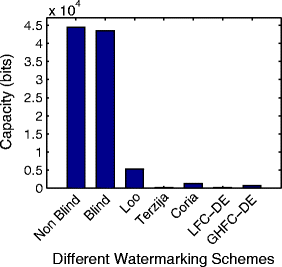

  

  Robustness comparison of different watermarking schemes after a formatting attack on the watermarked images. Capacities of the proposed non-blind and blind watermarking schemes are evaluated for the data-set (Fig. 11)

• Cropping.  Figure 26 gives the capacities of the proposed watermarking schemes after cropping the formatted watermarked images for different cropping percentages. Figure 26 depicts the following:

  • Increase in cropping percentage decreases capacities of non-blind and blind watermarking schemes.

  • Non-blind watermarking scheme has the highest robustness.

  • Blind watermarking scheme has the second highest robustness up to 30 percent cropping.

  Fig. 26

  

  Robustness comparison of different watermarking schemes after cropping the formatted watermarked images. Capacities of the proposed non-blind and blind watermarking schemes are evaluated for the data-set (Fig. 11)

• Gaussian filtering.  Figure 27 gives the capacities of the proposed watermarking schemes after Gaussian filtering the formatted watermarked images for different filter variances. Figure 27 depicts the following:

  • Filter variance does not affect the capacities of the proposed non-blind and blind watermarking schemes up to a filter variance of 0.3. After that, the filter variance drastically decreases the capacities of both watermarking schemes.

  • Non-blind watermarking scheme has the highest robustness up to a filter variance of 0.5.

  • Blind watermarking scheme has the second best robustness up to a filter variance of 0.5.

  • Filter variance saturates non-blind watermarking scheme capacity after a filter variance of 0.6. Moreover, the capacity of the non-blind watermarking scheme converges to the reported capacity of the Terzija et al. [39] scheme, Coria et al. [4] scheme, and LFC-DE and GHFC-DE [43] schemes after a filter variance of 0.6.

  Fig. 27

  

  Robustness comparison of different watermarking schemes after Gaussian filtering the formatted watermarked images. Capacities of the proposed non-blind and blind watermarking schemes are evaluated for the data-set (Fig. 11)

• Gaussian noise.  Figure 28 gives the capacities of the proposed watermarking schemes after adding Gaussian noise in the formatted watermarked images for different noise variances. Figure 28 depicts the following.

  • Increase in noise variance decreases the capacities of non-blind and blind watermarking schemes.

  • Non-blind watermarking scheme has the best robustness up to a noise variance of 5×10⁻⁵.

  • Blind watermarking scheme has the second best robustness up to a noise variance of 2×10⁻⁵.

  • Capacity of the blind watermarking scheme converges to the reported capacity of the Terzija et al. [39] scheme, Coria et al. [4] scheme, and LFC-DE and GHFC-DE [43] schemes, after a noise variance of 3×10⁻⁵.

  Fig. 28

  

  Robustness comparison of different watermarking schemes after adding Gaussian noise in the formatted watermarked images. Capacities of the proposed non-blind and blind watermarking schemes are evaluated for the data-set (Fig. 11)

• Salt and pepper noise.  Figure 29 gives the capacities of the proposed watermarking schemes after adding salt and pepper noise in the formatted watermarked images for different noise densities. Figure 29 depicts the following:

  • Increase in noise variance drastically decreases the capacities of non-blind and blind watermarking schemes.

  • Non-blind and blind watermarking schemes have the best robustness up to noise density of 0.05.

  • Non-blind watermarking scheme has the worst robustness from a noise density of 0.1.

  • Capacity of the blind watermarking scheme converges to the reported capacity of Terzija et al. [39] scheme, Coria et al. [4] scheme, and LFC-DE and GHFC-DE [43] schemes, after a noise density of 0.1.

  Fig. 29

  

  Robustness comparison of different watermarking schemes after adding salt and pepper noise in the formatted watermarked images. Capacities of the proposed non-blind and blind watermarking schemes are evaluated for the data-set (Fig. 11)

5 Conclusion

Non-blind and blind watermarking schemes have been developed in the ROWT domain. The proposed watermarking schemes have improved capacity and improved watermark length. The drastic improvement in the capacity and the length of the watermarks is achieved due to the observed property of the ROWT. Experiments are conducted on a data-set of six gray scale images and five meaningful binary logo watermarks. Experimental results reveal the following:

• The capacity of the proposed non-blind watermarking scheme and the visual quality of the corresponding watermarked images change with the embedding strength. We have observed that the embedding strength of a value near 3 is optimum for formatted watermarked images. Near optimum embedding strength, the capacity is at its maximum and formatted watermarked images are visually undistinguishable from corresponding original images.

• The performance of the blind watermarking scheme can be controlled by the embedding strength and the error controller. We have observed that the embedding strength and error controller pair is optimum near tuple of (5,0.25) for formatted watermarked images. Near an optimum pair, capacity is at its maximum and formatted watermarked images are visually undistinguishable from corresponding original images.

• Positive sub-bands can be used for a traditional non-blind watermarking scheme as extracted watermarks from positive sub-bands are very close to original watermarks. However, for a traditional blind watermarking scheme, extracted watermarks from all sub-bands are very noisy. Therefore, the observed property of the ROWT is significant for blind watermarking scheme and is slightly important for the non-blind watermarking scheme.

• We have tested both proposed watermarking schemes against various attacks such as cropping, Gaussian filter, Gaussian noise and salt and pepper noise. We have observed that the proposed non-blind and blind watermarking schemes have better robustness than existing DTCWT based watermarking schemes. Moreover, the proposed non-blind watermarking scheme has better robustness than the proposed blind watermarking scheme.

References

Agarwal H, Raman B, Venkat I (2014) Blind reliable invisible watermarking method in wavelet domain for face image watermark. Multimedia Tools and Applications. doi:10.1007/s11042-014-1934-1
Bhatnagar G, Raman B (2011) A new robust reference logo watermarking scheme. Multimedia Tools and Applications 52(2–3):621–640
Bhatnagar G, Wu QJ (2013) Biometrics inspired watermarking based on a fractional dual tree complex wavelet transform. Futur Gener Comput Syst 29(1):182–195
Coria LE, Pickering MR, Nasiopoulos P, Ward RK (2008) A video watermarking scheme based on the dual-tree complex wavelet transform. IEEE Transactions on Information Forensics and Security 3(3):466–474
Cox I, Miller M, Bloom J, Fridrich J, Kalker T (2007) Digital Watermarking and Steganography, 2nd edn. Morgan Kaufmann Publishers Inc., San Francisco
Cox IJ, Kilian J, Leighton FT, Shamoon T (1997) Secure spread spectrum watermarking for multimedia. IEEE Trans Image Process 6(12):1673–1687
Fallahpour M (2011) High capacity audio watermarking using the high frequency band of the wavelet domain. Multimedia tools and Applications 52(2–3):485–498
Gonde AB, Maheshwari RP Balasubramanian R (2010) Complex wavelet transform with vocabulary tree for content based image retrieval. In: Proceedings of the Seventh Indian Conference on Computer Vision, Graphics and Image Processing, ACM, Chennai
Gonzalez RC, Woods RE (2008) Digital Image Processing. Prentice Hall
Holliman M, Memon N (2000) Counterfeiting attacks on oblivious block-wise independent invisible watermarking schemes. IEEE Trans Image Process 9(3):432–441
Jain AK, Uludag U (2003) Hiding biometric data. IEEE Transactions on Pattern Analysis and Machine Intelligence 25(11):1494–1498
Khana A, Malika SA, Alib A, Chamlawia R, Hussaina M, Mahmoodc MT, Usmand I (2012) Intelligent reversible watermarking and authentication: Hiding depth map information for 3d cameras. Elsevier, Inf Sci 216:155–175
Kim WG, Lee HK (2009) Multimodal biometric image watermarking using two-stage integrity verification. Sig Process 89(12):2385–2399
Kokare M, Biswas PK, Chatterji BN (2005) Texture image retrieval using new rotated complex wavelet filters. IEEE Transactions on Systems, Man, and Cybernetics Part B: Cybernetics 35(6):1168–1178
Kokare M, Biswas PK, Chatterji BN (2006) Rotation-invariant texture image retrieval using rotated complex wavelet filters. IEEE Transactions on Systems, Man, and Cybernetics Part B: Cybernetics 36(6):1273–1282
Korus P, Białas J, Dziech A (2012) A new approach to high-capacity annotation watermarking based on digital fountain codes. Multimedia Tools and Applications: 1–19
Kumar S, Kumar S, Raman B, Sukavanam N (2013) Image disparity estimation based on fractional dual-tree complex wavelet transform: A multi-scale approach. International Journal of Wavelets. Multiresolution and Information Processing 11(1):1350,004,1–1350,004,21
Kundur D, Hatzinakos D (1999) Digital watermarking for telltale tamper proofing and authentication. Proceedings of IEEE 87(7):1167–1179
Kundur D, Hatzinakos D (2004) Toward robust logo watermarking using multiresolution image fusion principles. IEEE Trans Multimed 6(1):185–198
Li CT, Yang FM, Lee CS (2002) Oblivious fragile watermarking scheme for image authentication. IEEE International Conference on Acoustics, Speech, and Signal Processing 4:IV–3445 – IV–3448
Lina TC, Linb CM (2009) Wavelet-based copyright-protection scheme for digital images based on local features. Elsevier, Inf Sci 179(19):3349–3358
Loo P, Kingsbury NG (2000) Digital watermarking using complex wavelets. In: International Conference Image Processing, IEEE, Vancouver, vol 3
Ma B, Wang Y, Li C, Zhang Z, Huang D (2013) Secure multimodal biometric authentication with wavelet quantization based fingerprint watermarking. Multimedia Tools and Applications. doi: 10.1007/s11042-013-1372-5
Magarey J, Kingsbury NG (1998) Motion estimation using a complex-valued wavelet transform. IEEE Transactions on Signal Processing 46(4):1069–1084
Mallat SG (1989) A theory for multiresolution signal decomposition: The wavelet representation. IEEE Transactions on Pattern Analysis and Machine Intelligence 2(7):674–693
Miller M, Kingsbury N, Hobbs R (2005) Seismic imaging using complex wavelets. In: Proceeding of International Conference on Acoustic, Speech, Signal Processing (ICASSP), IEEE, Philadelphia, vol 2
Mohanty SP (2009) A secure digital camera architecture for integrated real-time digital rights management. J Syst Archit 55(10):468–480
Mohanty SP, Ramakrishnan KR, Kankanhalli MS (2000) A dct domain visible watermarking technique for images. IEEE International Conference on Multimedia and Expo 2:1029–1032
Ramkumar M, Akansu AN (1998) Information theortic bounds for data hiding in compressed images. In: IEEE Second Workshop on Multimedia Signal Processing
Rani A, Raman B, Kumar S (2013) A robust watermarking scheme exploiting balanced neural tree for rightful ownership protection. Multimedia Tools and Applications: 1–24
Romberg J, Choi H, Baraniuk R, Kingsbury N (2000) Multiscale classification using complex wavelets and hidden markov tree models. In: Proceeding International Conference Image Processing, Vancouver, vol 2
Selesnick I (2014) 2-d dual-tree wavelet transform. http://eeweb.poly.edu/iselesni/WaveletSoftware/dt2D.html, last accessed on April, 2014
Selesnick IW, Baraniuk RG, Kingsbury NG (2005) The dual-tree complex wavelet transform. IEEE Signal Procesing Magazine: 123–151
Shaffrey CW, Kingsbury NG, Jermyn IH (2002) Unsupervised image segmentation via markov trees and complex wavelets. In: Proceedings of Internationl Conference on ImageProcessing, IEEE, Rochester, vol 3
Shia X, Xiaoa D (2013) A reversible watermarking authentication scheme for wireless sensor networks. Elsevier, Inform Sci 240:173–183
Skodras A, Christopoulos C, Ebrahimi T (2001) The jpeg 2000 still image compression standard. IEEE Signal Procesing Magazine: 36–58
Suhail M, Obaidat M, Ipson S, Sadoun B (2003) A comparative study of digital watermarking in jpeg and jpeg 2000 environments. Elsevier, Inform Sci 15:93–105
Tang CW, Hang HM (2003) A feature-based robust digital image watermarking scheme. IEEE Transactions on Signal Processing 51(4):950–959
Terzija N, Geisselhardt W (2004) Digital image watermarking using complex wavelet transform. In: Proceeding Workshop Multimedia Security, ACM, Magdeburg
Wallace GK (1992) The jpeg still picture compression standard. IEEE Trans Consum Electron 38(1):18–34
Wang N, Men C (2013) Reversible fragile watermarking for locating tampered blocks in 2d vector maps. Multimedia Tools and Applications 67(3):709–739
Wong PW, Memon N (2001) Secret and public key image watermarking schemes for image authentication and ownership verification. IEEE Trans Image Process 10(10):1593–1601
Yang H, Jiang X, Kot AC (2011) Embedding binary watermarks in dual-tree complex wavelets domain for access control of digital images. Springer, Transactions on DHMS 6:18–36
Ye Z, Lu CC (2003) A complex wavelet domain markov model for image denoising. In: Proceedings of International Conference on Image Processing, IEEE, Barcelona, vol 3
Acknowledgment
One of the authors, Himanshu Agarwal, acknowledges the University Grants Commission (UGC) of New Delhi, India for granting him a scholarship under the JRF scheme for his research. He also acknowledges the grant from the Canadian Bureau for International Education under the Canadian Commonwealth Scholarship Program.
Author information
Authors and Affiliations
Corresponding author
Rights and permissions
About this article
Cite this article
Agarwal, H., Atrey, P.K. & Raman, B. Image watermarking in real oriented wavelet transform domain. Multimed Tools Appl 74, 10883–10921 (2015). https://doi.org/10.1007/s11042-014-2212-y
Received:
Revised:
Accepted:
Published:
Issue Date:
DOI: https://doi.org/10.1007/s11042-014-2212-y