
Abstract
In this paper we investigate multilevel programming problems with multiple followers in each hierarchical decision level. It is known that such type of problems are highly non-convex and hard to solve. A solution algorithm have been proposed by reformulating the given multilevel program with multiple followers at each level that share common resources into its equivalent multilevel program having single follower at each decision level. Even though, the reformulated multilevel optimization problem may contain non-convex terms at the objective functions at each level of the decision hierarchy, we applied multi-parametric branch-and-bound algorithm to solve the resulting problem that has polyhedral constraints. The solution procedure is implemented and tested for a variety of illustrative examples.
1 Introduction
Multilevel programming problems are nested optimization problems in which part of the constraint set is determined by the solution sets of another optimization problems, so-called follower’s problems. These kind of problems are common in divers application areas [7, 9, 10, 21, 34]. However, multilevel programming problems are non-convex and quite difficult to deal with even for their linear formulations [8, 23, 34]. In proposing solution mechanisms to such kind of problems, most of the methods proposed so far assume that the functions involved in the model are linear or strictly convex so that the reaction of the followers at each stage can be determined uniquely [21, 23, 31, 35]. In practice, however, there are several problems that require a nonconvex structure also at lower level problems. For instance, the utility functions at the lower levels could be nonconvex and sometimes stochastically noisy. Moreover, in allocation of healthcare resources the models of the diseases to be combated at the lower levels are usually nonconvex in their nature. The solution for hierarchical problems in general are obtained at the Stackelberg equilibrium point in the vertical decision structure.
Moreover, many practical problems could be modeled as multilevel programs having multiple decision makers at the same level over the hierarchy and are called multilevel programs with multiple followers [7, 22]. Using the common notation in multilevel programming, such kind of problems can be stated mathematically as:

where \(y_{1}\in Y_{1}\subset {\mathbb {R}}^{n_1}\) is a decision vector for the leader’s optimization problem whereas, \(y_m^c\in Y_m^c\subset {\mathbb {R}}_m^{n_c}\) is a decision vector for the cth follower at level m, and \(y_m^{-c}\) is a vector of the decision variables for all followers at the level m without the decision variables \(y_m^c\), of follower c. i.e., \(y_m^{-c} = (y_m^1,\ldots ,y_m^{c-1},y_m^{c+1},\ldots ,y_m^n)\), where, \(c=i,j,\ldots ,l\) and \(m\in \{2,3,\ldots ,k\}\). The shared constraint \(h_m\) is the mth level followers common constraint set whereas, the constraint \(g_m^i\) determines the constraint only for the ith follower at the mth level optimization problem. Throughout this paper, it is assumed that \(F, ~G, ~f_m^c, ~h_m\) and \(g_m^c\) are twice continuously differentiable functions.
One can easily see a bilevel program with multiple followers in problem (1.1) by setting \(m=2\) and can be described as:

The ith follower problem in (1.2) could be seen as a multi-parametric programming problem (for a given strategy \(y_1\)), by considering the optimization variables from other followers as parameters. But, the main difficulty with this problem is that an individual decision maker does not know the choice, \(y_2^{-i}\), of the other followers. This further increases the complexity of problem (1.2) in addition to its implicit structure.
Even if it is not a generic assumption, it has been assumed in many papers that the ith follower knows the strategies \(y_2^{-i}\) of other followers. For example, Faísca et al. [17] have proposed a solution approach to the special case of problem (1.2) by considering the ith follower as a multi-parametric programming problem where, the leader’s and the rest of the followers optimization variables are considered as parameters. The algorithm uses a parametric comparison approach to compute a Nash equilibrium reaction.
Using strong constraint qualification assumptions, Wang et al. [36] have proposed an approach to solve problem (1.2) after replacing the followers problem with its concatenated KKT conditions based on the idea of vertex searching without the complementarity constraints, while the gradient of the followers objective function is linear and the followers constraint set is defined by linear functions. Moreover, the leader’s optimization problem is considered as strictly convex. However, this approach could not be extended to solve general k-level programs with multiple followers, because there exist non-convex terms and shared variables across the followers at the \(k-1\) level due to complementarity conditions from the kth level followers. This may result in non-solvable multilevel program with multiple followers having shared variables (which means the approach is restricted only for bilevel programs with multiple followers).
In general, solving a multilevel program having multiple followers at each decision level is quite difficult and complex when there is information exchange between followers. Thus, it would be interesting to identify a class of problem (1.1) which can be reformulated as a multilevel program having single follower at each decision level. In Calvete et al. [9] and Bard [5] problem (1.2) has been reformulated equivalently as a bilevel program with single follower. The two papers are devoted for bilevel programs with independent followers (i.e., One of the follower does not affect the decision of the other follower and vice-versa). In practice however, there could be communication and sharing of resources between followers at the same level of decision.
Wang et al. [36] have reformulated a bilevel program with multiple follower into an equivalent bilevel program with single follower when there is information exchange (If one follower tries to alter his/her strategy, he/she can not improve his/her own objective) and resource sharing across the followers. The discussion of the paper pays attention for the case in which the objective functions of each of the followers should be separable in the sense that, \(f_i(y_1,y_2^i,y_2^{-i}) = f_i^1(y_1,y_2^i) + f_2^i(y_1,y_2^{-i})\) for \(i = 1,2,\ldots ,I\). However, in some real applications, the followers problem in (1.1) may have implicit formulation of non-separability while keeping its convexity with respect to its own decision variable.
In this paper we reformulate the class of multilevel programs with multiple followers, that consist of separable terms and parameterized common terms across all the followers, into equivalent multilevel programs having single follower at each level of decision and propose an efficient method of solving the resulting problem. The proposed solution approach can solve multiple-follower problems whose objective values have common, but having different positive weights of, nonseparable terms. The rest of the paper is organized as follows; in Sect. 2 the relation between some classes of multilevel programs with multiple followers and multilevel programs with single followers is discussed and described briefly. Section 3 suggests appropriate solution methods to the reformulated multilevel programm with single followers and some numerical examples are provided to illustrate the approach in Sect. 4. Finally, the paper ends with concluding remarks in Sect. 5.
2 Relation between multilevel programs with multiple followers and multilevel programs with single followers
In this Section, we will consider the possibilities of reformulating some classes of multilevel programs with multiple followers as multilevel programs having only single follower at each level of the hierarchy. For the sake of clarity in presentation, the methodology is described using bilevel programs with multiple followers and trilevel programs with multiple followers, however it can be extended to general k-level hierarchical programs with multiple followers at each level of decision.
2.1 Relations between some classes of bilevel programs with multiple followers and bilevel programs with single follower
Let us consider each objective function in problem (1.2) consisting of separable terms and parameterized common terms across all followers with positive weights \(\rho \in \mathbb {R}^{I}_+\), that is, \(f_2^i (y_1,y_2^i,y_2^{-i}) = f_2^i (y_1,y_2^i)+f_2^i (y_1,y_2^{-i})+\rho ^i\tilde{f} (y_1,y_2^i,y_2^{-i})\), with \(\rho ^i > 0\) for each \(i = 1,2,\ldots ,I\). Thus, problem (1.2) can be reformulated as:

Let us assume that the followers constraint functions satisfy some constraint qualification conditions (for instance, the Guignard constraint qualifications conditions) and to make the presentation clear, let us define some relevant sets as follows:
-
(i)
The set \(\varOmega = \{(y_1,y_2^i,y_2^{-i}):G(y_1,y_2^i,y_2^{-i})\le 0,~h (y_1,y_2^i,y_2^{-i})\le 0,~ g_2^i (y_1,y_2^i) \le 0 \}\) is called the constraint set of problem (2.1)
-
(ii)
The feasible set for the ith follower (for any strategy \(y_1\) of the leader’s problem) can be defined as, \(\varOmega _i (y_1,y_2^{-i})=\{y_2^i:h_2 (y_1,y_2^i,y_2^{-i})\le 0,~ g_2^i(y_1,y_2^i)\le 0\}\)
-
(iii)
The set \(RR_2^i (y_1,y_2^{-i}) = \{y_2^i:y_2^i\in \arg \min \{f_2^i (y_1,y_2^i,y_2^{-i}):h_2 (y_1,y_2^i,y_2^{-i})\le 0,~ g_2^i (y_1,y_2^i)\le 0\}\}\) is the Nash rational reaction set for the ith follower
-
(iv)
Projection of the feasible set \(\varOmega \) onto the leader’s decision space can be defined as: \(\varOmega (y_1)=\{y_1:\exists (y_2^i,y_2^{-i}): G (y_1,y_2^i,y_2^{-i})\le 0,~h_2 (y_1,y_2^i,y_2^{-i})\le 0,~ g_i (y_1,y_2^i)\le 0\}\)
-
(v)
The set \(\mathcal {I\!R} = \{(y_1,y_2^i,y_2^{-i}):(y_1,y_2^i,y_2^{-i})\in \varOmega , y_2^i\in RR_2^i(y_1,y_2^{-i}), i=1,2,\ldots ,I\}\) is called the inducible set or feasible set for the leader’s problem.
We also assume that \(\mathcal {I\!R}\) is non-empty to guaranty the existence of a solution to problem (2.1). With these definitions of sets and assumptions, problem (2.1) can be rewritten as:
On the other hand, suppose that \(f_2^i\), \(g_2^i\) and \(h_2\) are convex with respect to \(y_2^i\), for each \(i = 1,2,\ldots ,I\), and if the Guignard constraint qualification hold [20] at the optimal Nash equilibrium point \((y_1^*,y_2^{i,*},y_2^{-i,*})\). Then as can be seen in [36] \((y_1^*,y_2^{i,*},y_2^{-i,*})\) solves the following non-convex optimization problem and conversely.

The description given above shows that problem (2.3) and (2.2) are equivalent to problem (2.1). The following discussion gives a good understanding on the relation between single follower bilevel programming problems and bilevel programs with multiple followers based on the above results.
Now let us consider the following bilevel program with single follower:

Note that the terms \(f_2^i (y_1,y_2^{-i})\) for \(i=1,2,\ldots ,I\) are omitted in problem (2.4) because, they are constant functions with respect to \(y_2^i\) at the followers problem in (2.1) and hence they do not contribute to the optimization process.
Here again let us define some sets corresponding to problem (2.4) as follows:
-
(a)
The set \(S=\varOmega \) is the feasible set of problem (2.4)
-
(b)
The set \(S_L(y_1) = \{(y_2^i,y_2^{-i}):g_2^i (y_1,y_2^i)\le 0,~h_2 (y_1,y_2^i,y_2^{-i})\le 0,i=1,2,\ldots ,I\}\) defines the feasible set of the second level problem in (2.4).
-
(c)
The set \(\varPsi (y_1) = \left\{ (y_2^i,y_2^{-i}): (y_2^i,y_2^{-i})\in \arg \min \left\{ \left[ \sum _{i=1}^I\frac{1}{\rho ^i}f_2^i (y_1,y_2^i)\right] \right. \right. + \left. \left. \tilde{f}(y_1,y_2^i,y_2^{-i}): (y_2^i,y_2^{-i})\in S_L(y_1)\right\} \right\} \) is the rational reaction set of the second level decision maker in problem (2.4)
-
(d)
The set \(\mathcal {I\!R}_S = \{(y_1,y_2^i,y_2^{-i}):(y_1,y_2^i,y_2^{-i})\in \varOmega , (y_2^i,y_2^{-i})\in \varPsi (y_1)\}\) denotes the inducible region.
Based on the definitions of sets given above, a bilevel programming problem (2.4) can be rewritten as:
Theorem 2.1
Problem (2.1) is equivalent to problem (2.4).
Proof
In order to prove the equivalence of the two problems it is enough to show \(\mathcal {I\!R} = \mathcal {I\!R}_S\), because the objective functions in (2.2) and (2.5) are identically similar. To this end, let \((\bar{y}_1,\bar{y}_2^i,\bar{y}_2^{-i})\in \mathcal {I\!R}\). Hence, \((\bar{y}_1,\bar{y}_2^i,\bar{y}_2^{-i})\in \varOmega ~\text {and}~ \bar{y}_2^i\in RR_2^i (\bar{y}_1,\bar{y}_2^{-i}), i=1,2,\ldots ,I.\) Suppose that \((\bar{y}_2^i,\bar{y}_2^{-i})\) is not an optimal solution to the second level problem in (2.4) for \(y_1=\bar{y}_1\), then \(\exists (y_2^{*i},\bar{y}_2^{-i})\in S_L(\bar{y}_1)\) such that
But, since \((y_2^{*i},\bar{y}_2^{-i})\in S_L (\bar{y}_1)\), then \(y_2^{*i}\in \varOmega _i(\bar{y}_1,\bar{y}_2^{-i}), i= 1,2,\ldots ,I\). This implies that,
Which contradicts inequality (2.6). Hence, \((\bar{y}_1,\bar{y}_2^i,\bar{y}_2^{-i})\in \mathcal {I\!R}_S\).
Conversely, let \((\bar{y}_1,\bar{y}_2^i,\bar{y}_2^{-i})\in \mathcal {I\!R}_S\). This implies that, \((\bar{y}_1,\bar{y}_2^i,\bar{y}_2^{-i})\in \varOmega \), \((\bar{y}_1,\bar{y}_2^i,\bar{y}_2^{-i})\in S_L(\bar{y}_1)\), and \(\bar{y}_2^i\in \varOmega _i (\bar{y}_1,\bar{y}_2^{-i}), i=1,2,\ldots ,I.\) If there exist at least one \(j\in \{1,2,\ldots ,I\}\) such that \(\bar{y}_2^j \notin RR_2^j(\bar{y}_1,\bar{y}_2^{-j})\), then \(\exists y_2^{*j}\in \varOmega _j(\bar{y}_1,\bar{y}_2^{-j})\) such that the following holds;
where \(y_2^{*j}\) refers to an optimal solution of the jth follower problem in (2.1) for \(y_1=\bar{y}_1\). But, since \((\bar{y}_1,y_2^{*j},\bar{y}_2^{-j})\in S_L(\bar{y}_1)\) and \((\bar{y}_1,\bar{y}_2^j,\bar{y}_{2}^{-j})\) is an optimal solution to the second level of problem (2.4) for \(y_1=\bar{y}_1\), then we have
This implies, \(\frac{1}{\rho ^j}f_2^j (\bar{y}_1,\bar{y}_2^j)+\frac{1}{\rho ^j} f_2^j (\bar{y}_1,\bar{y}_2^{-j})+\tilde{f}(\bar{y}_1, \bar{y}_2^j,\bar{y}_2^{-j})\le \frac{1}{\rho ^j}f_2^j (\bar{y}_1,y_2^{j*})+ \frac{1}{\rho ^j}f_2^j (\bar{y}_1,\bar{y}_2^{-j})+ \tilde{f} (\bar{y}_1, y_2^{j*},\bar{y}_{2}^{-j})\), which contradicts equation (2.7). Hence, \((\bar{y}_1,\bar{y}_2^i,\bar{y}_2^{-i})\in \mathcal {I\!R}\)
Alternative Proof: On the other hand, it is enough to see problem (2.4) has a form similar to problem (2.3). Now since, the follower’s problem are all convex and the constraints in (2.4) are assumed to satisfy the Guignard constraint qualifications at \(y_2^i\), the Karush-Kuhn-Tucker conditions can be used to obtain

Since \(\rho > 0\) and \( \lambda \rho = \lambda ^0 \ge 0\), we can reformulate problem (2.8) as

Now by setting \(\lambda ^0=\rho \lambda \) and \(\eta ^i = \mu ^i\rho ^i\), we see that (2.9) is equivalent to problem (2.3) with Lagrange multipliers \(\lambda ^0\) and \(\eta ^i \). \(\square \)
2.2 Relation between classes of trilevel programming problems with multiple followers and hierarchical trilevel programming problems
Consider the following trilevel programming problem with multiple followers at the two lower levels and in which the followers objective functions have the form as discussed in Sect. 2.1. That is:

A1: Assume that each of the objective functions is convex with respect to its own decision variable vector for the third and second level followers and the Guignard constraint qualifications hold for the followers constraints.
To proceed the presentation let us define the following sets,
-
1.
The set
$$\begin{aligned} \varOmega _3\left( y_1,y_2^i,y_2^{-i},y_3^{-j}\right) =\left\{ y_3^j \in Y_3^j:g_3^j\left( y_1,y_2^i,y_2^{-i},y_3^j\right) \le 0,~h_3\left( y_1,y_2^i,y_2^{-i},y_3^j,y_3^{-j}\right) \le 0\right\} \end{aligned}$$is called a feasible set for the third level followers problem.
-
2.
The set of parametric solutions defined by,
$$\begin{aligned} \varPsi _3\left( y_1,y_2^i,y_2^{-i},y_3^{-j}\right)= & {} \left\{ \bar{y}_3^j \in Y_3^j: \bar{y}^j_3 \in \arg \min \left\{ f_3^j\left( y_1,y_2^i,y_2^{-i},y_3^j,y_3^{-j}\right) :\right. \right. \\&\left. \left. \quad y^j_3\in \varOmega _3\left( y_1,y_2^i,y_2^{-i},y_3^{-j}\right) \right\} , ~j=1,2,\ldots ,J\right\} \end{aligned}$$is called the rational reaction set for the third level followers problem.
-
3.
The set
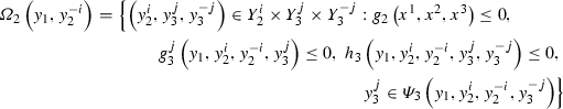
is called a feasible set for the second level problem.
-
4.
The set of solutions
$$\begin{aligned} \varPsi _2\left( y_1,y_2^{-i}\right)= & {} \left\{ \left( y_2^i,y_3^j,y_3^{-j}\right) \in Y_2^i\times Y_3^j\times Y_3^{-j}: \right. \\&\quad \quad y_2^i\in \arg \min \left\{ f_2^i\left( y_1,y_2^i,y_2^{-i},y_3^j,y_3^{-j}\right) : \right. \\&\left. \left. \quad \qquad \left( y_2^i,y_3^j,y_3^{-j}\right) \in \varOmega _2\left( y_1,y_2^{-i}\right) , i = 1,2,\ldots ,I\right\} \right\} \end{aligned}$$is called the rational reaction set for the second level followers problem.
-
5.
The set
$$\begin{aligned} \varPhi= & {} \left\{ \left( y_1,y_2^i,y_2^{-i},y_3^j,y_3^{-j}\right) : g^j_3\left( y_1,y_2^i,y_2^{-i},y_3^j \right) \le 0, h_3\left( y_1,y_2^i,y_2^{-i},y_3^j,y_3^{-j}\right) \le 0,\nonumber \right. \\&\qquad g^i_2\left( y_1,y_2^i,y_2^{-i},y_3^j \right) \le 0, h_2\left( y_1,y_2^i,y_2^{-i},y_3^j,y_3^{-j}\right) \le 0, \nonumber \\&\left. \qquad G\left( y_1,y_2^i,y_2^{-i},y_3^j,y_3^{-j} \right) \le 0\right\} \end{aligned}$$(2.11)is called the feasible set of problem (2.10)
-
6.
The region
$$\begin{aligned} {\mathcal {I\!R}}= & {} \left\{ \left( y_1,y_2^i,y_2^{-i},y_3^j,y_3^{-j}\right) :\left( y_1,y_2^i,y_2^{-i},y_3^j,y_3^{-j}\right) ~\right. \\&\left. \in \varPhi ,~\left( y_2^i,y_2^{-i},y_3^j,y_3^{-j}\right) ~ \in ~ \varPsi _2\left( y_1,y_2^{-i}\right) \right\} \end{aligned}$$is called the inducible region

Considering the above sets, problem (2.10) could be rewritten as:
Consider the following hierarchical trilevel programming problem having single decision maker at each decision level:

In problem (2.13) the terms \(f_2^i(y_1,y_2^{-i},y_3^j,y_3^{-j})\) and \(f_3(y_1,y_2^i,y_2^{-i},y_3^{-j})\) at the second and third level respectively are omitted because, they are constant with respect to \(y_2^i\) and \(y_3^j\) which means they do not contribute to the optimal decision at the ith and jth followers of the second and third level in problem (2.10)
Similarly, we can define some sets related to problem (2.13) as follows:
-
1.
The set
$$\begin{aligned} \varphi _3\left( y_1,y_2^i,y_2^{-i}\right)= & {} \left\{ \left( y_3^j,y_3^{-j}\right) \in Y_3^j\times Y_3^{-j}: \right. \\&g_3^j\left( y_1,y_2^i,y_2^{-i},y_3^j\right) \le 0, \\&\left. h_3\left( y_1,y_2^j,y_2^{-j},y_3^j,y_3^{-j}\right) \le 0,(j=1,2,\ldots ,J) \right\} \end{aligned}$$is called a feasible set for the third level.
-
2.
The set of parametric solutions defined by,

is called the rational reaction set for the third level.
-
3.
The set
$$\begin{aligned} \varphi _2(y_1)= & {} \left\{ \left( y_2^i,y_2^{-i},y_3^j,y_3^{-j}\right) \in Y_2^i\times Y_2^{-i}\times Y_3^j\times Y_3^{-j}: \right. \\&g_2^i\left( y_1,y_2^i,y_3^j, y_3^{-j}\right) \le 0, h_2\left( y_1,y_2^i,y_2^{-i},y_3^j,y_3^{-j}\right) \le 0, \\&g_3^j\left( y_1,y_2^i,y_2^{-i},y_3^j\right) \le 0, h_3\left( y_1,y_2^i,y_2^{-i},y_3^j,y_3^{-j}\right) \le 0,\\&\left. \left( y_3^j,y_3^{-j}\right) \in \psi _3\left( y_1,y_2^i,y_2^{-i}\right) \right\} \end{aligned}$$is called a feasible set for the second level problem.
-
4.
The set of solutions

is called the rational reaction set for the second level, for \(X_i \subseteq \mathbb {R}^{n_i}, i = 1,2,3\).
-
5.
The set \(\digamma = \varPhi \) (which is defined in Equation (2.11)) is the feasible set for problem (2.13).
-
6.
The set \(\mathcal {I\!R}_3 = \{(y_1,y_2^i,y_2^{-i},y_3^j,y_3^{-j}):(y_1,y_2^i,y_2^{-i},y_3^j,y_3^{-j})\in \digamma , (y_2^i,y_2^{-i},y_3^j,y_3^{-j})\in \psi _2 (y_1)\}\)


Using the definitions described above, the hierarchical problem (2.13) can be rewritten as follows:
Theorem 2.2
Problem (2.14) and (2.12) are equivalent.
Proof
Let \((\bar{y}_1,\bar{y}_2^i,\bar{y}_2^{-i},\bar{y}_3^j,\bar{y}_3^{-j})\in \mathcal {I\!R}_3\). This implies \((\bar{y}_2^i,\bar{y}_2^{-i})\) and \((\bar{y}_3^j,\bar{y}_3^{-j})\) minimizes the second and third level problems in (2.13) respectively. Let \((\bar{y}_1,\bar{y}_2^i,\bar{y}_2^{-i},\bar{y}_3^j,\bar{y}_3^{-j})\notin \mathcal {I\!R}\), then there exist at least one \(k\in \{1,2,\ldots ,J\}\) and \(p\in \{1,2,\ldots ,I\},\) respectively, such that \(\bar{y}_3^k\notin \varPsi _3(\bar{y}_1,\bar{y}_2^i,\bar{y}_2^{-i}, \bar{y}_3^{-k})\) and \(\bar{y}_2^p\notin \varPsi _2(\bar{y}_1,\bar{y}_2^{-p})\). This implies the following:
and
where, \(y_3^{*k}\) and \(y_2^{*p}\) are optimal solutions for the third level (kth follower) and second level (pth follower) respectively. Since \(y_3^{*k}\) minimizes the kth follower problem of the third level, we have \(y_3^{*k}\in \varPsi _3(\bar{y}_1,\bar{y}_2^i,\bar{y}_2^{-i},y_3^{-k})\) which implies \(y_3^{*k}\in \varphi _3(\bar{y}_1,\bar{y}_2^i,\bar{y}_2^{-i})\) and hence, \((y_3^{*k},\bar{y}_3^{-k})\in \varphi _3(\bar{y}_1,\bar{y}_2^i,\bar{y}_2^{-i})\) and similarly, \((y_2^{*p},\bar{y}_2^{-p},\bar{y}_3^{j},\bar{y}_3^{-j})\in \varphi _2(\bar{y}_1)\) as well. Moreover, we know that \((\bar{y}_3^j,\bar{y}_3^{-j})\) is an optimal solution to the third level subproblem in (2.13) for a given point \((\bar{y}_1,\bar{y}_2^i,\bar{y}_2^{-i})\), then we have the following
which implies
which contradicts equation (2.15) and hence \((\bar{y}_1,\bar{y}_2^i,\bar{y}_2^{-i},\bar{y}_3^j,\bar{y}_3^{-j})\in \mathcal {I\!R}\) .
Similarly, if \((\bar{y}_2^i,\bar{y}_2^{-i})\) is an optimal solution to the second level subproblem in (2.13), then we have the following

which implies
which contradicts (2.16) and hence \((\bar{y}_1,\bar{y}_2^i,\bar{y}_2^{-i},\bar{y}_3^j,\bar{y}_3^{-j}) \in \mathcal {I\!R}\). \(\square \)
Remark 1
The alternative proof we described in Theorem 2.1 which is common in literature (see for instance [28]) does not work for the proof of Theorem 2.2. Moreover, the Lagrange multipliers of the third level followers are considered as shared variables for the second level followers. Further, the reformulated problem will be non-convex due to the complementarity condition. As a consequence, the resulting non-convex bilevel program with multiple followers may not have a Nash equilibrium reaction solution.
Remark 2
The idea described above can be extended to any finite k-level optimization problem with multiple followers while the objective function at each level has similar form as in problem (2.10).
3 Solution procedure
In this section we suggest an appropriate solution method to solve the resulting multilevel program with a single follower at each decision level. And we introduce a pseudo algorithmic approach to solve some classes of multilevel programs with multiple followers.
-
Step 1.
Reduce the given multilevel program with multiple followers equivalently into multilevel program having only single follower at each decision level as discussed in Sect. 2
-
Step 2.
If the followers objective functions as well as the common constraint (h) are separable (i.e., both have a form like \(f_m^c(y_1,y_m^c,y_m^{-c})=f_m^c(y_1,y_m^c)+f_m^c(y_1,y_m^{-c})\), where \(m=2,3,\ldots ,k\); \(c = i,j,\ldots ,l\)) and convex functions with respect to their own decision variables at each decision level, the reduced problem has convex follower at each decision level. In this case, we should apply one of the proposed algorithms described in [16, 23, 24, 30, 31, 38]. However, these approaches are suitable for bilevel programming problems and it seems too difficult to extend such an approach beyond two levels, because of the non-convex constraints introduced due to complementarity conditions. For general k-level multilevel programming problems having convex quadratic objective function and affine constraints at each decision level, we should use the algorithm proposed by Faísca et al. [17].
-
Step 3.
However, we may have implicit formulation at the objective functions of followers keeping convexity in its own decision variable. In this case, the resulting equivalent multilevel program with single follower (as in Sect. 2.2) is non-convex because the problem is optimized over the whole variables as can be seen in (2.4) and (2.13). And hence, we can apply the algorithm proposed in [21] for the bilevel case. However, here again it seems difficult to extend such an approach to general k-level multilevel programming problems because of the non-convex constraints introduced due to complementarity conditions. As a result, one should apply the algorithm proposed in [27] for general k-level programming problems with polyhedral constraints. In this paper the latest algorithm is implemented for the examples in the next section. Though the detail procedures of the algorithm is described in [27], here some basic steps are described.
Basic steps of the proposed algorithm
Given a k-level optimization problem with multiple followers as in equation (1.1) where the constraints at each level are polyhedral. Then to solve this problem we proceed as in the follows steps:
-
(i)
Convert the problem into its equivalent k-level problem with single follower as described in Sect. 2.2.
-
(ii)
Consider the kth level optimization problem of the converted problem in step (i) above as multi-parametric programming problem where, the variables from upper level decision makers are considered as parameters. Reduce it into standard non-convex optimization problem by fixing a feasible value to the parameters.
-
(iii)
Find a tight underestimator sub-problem using the branch-and-bound algorithm (described in [27]) and apply a multi-parametric programming approach to obtain a parametric solution and corresponding parametric regions in which the obtained solutions remain optimal. Repeat (i) and (ii) until the entire parametric region has been explored successfully.
-
(iv)
Incorporate the solutions and the corresponding regions into the \((k-1)\)-level problem and again consider it as a multi-parametric programming problem where, the upper levels’ decision variables are considered as parameters. Repeating the above procedures [(i), (ii) and (iii)] one can reach at the leader’s optimization problem.
4 Numerical experiment
Example 1
Consider the following linear bilevel program with three followers

The problem in this example is relatively simple. Since each of the three followers are separable functions and hence the resulting equivalent bilevel programm with a single follower is also simple which can be formulated as follows:

Reformulating the follower’s decision maker in problem (4.2) as a parametric programming problem where, x is considered as a parameter, it can be formulated as,

Since problem (4.3) is linear, there is no need of convexification of the problem and one can solve it globally as discussed in [16, 17]. As a result, we have solved problem (4.3) and obtained a parametric solution described as follows:
and problem (4.3) is infeasible for \(x>10\), because if \(x>10\) the inequality, \(3x + 3y_1 \le 30\) can not be satisfied unless \(y_1<0\), but the fact is that all the y values are assumed to be non-negative.
Incorporate the expression (4.4) into the leader’s problem to obtain a single level convex optimization problem. Solving the resulting problem we arrive at the following result \((x,y_1,y_2,y_3) = (5,5,10,5\)) with \(F=-35\) corresponding to \(CR^R_1\) which is similar to the result reported in [17].
Example 2
The second test problem is a bilevel program with two followers having bilinear forms as described here below:

The followers’ objectives in problem (4.5) can be reduced to a single follower by multiplying \(f_1\) by \(\frac{1}{2}\) and add it with the separable part of \(f_2\) to get
as the resulting nonseparable term \(-y_1y_2\) becomes common to both the followers. Then, the above problem can be reformulated as minimization problem as follows,

Problem (4.6) has a single follower with quadratic and bilinear formulation at the objective function. This formulation can result in multiple Nash equilibrium reaction for at least one feasible choice of the leader’s problem. To overcome this ambiguity we should apply a mathematical procedure described in [27]. Hence, one can treat the follower’s problem as a parametric programming problem by considering x as a parameter and it can be described as follows,

Solving problem (4.7) using the algorithm proposed in [27], one can obtain the following approximate parametric solutions with corresponding critical regions,

and problem (4.7) is infeasible for \(x > 2\). Incorporating each of the above solution expressions into the leader’s problem, one can get two bounded optimization problems. After solving the resulted problems, we have got best solution \((x,y_1,y_2) = (1,0,2)\) with corresponding values \(F = 23, f_1 = 0\), and \(f_2 = 8\) which is a similar (even it is better in terms of the followers response) solution as compared to the result reported in [36], which was, \(F = 22.5, f_1 = 0,\) and \(f_2 = 6.75\).
Example 3
Consider the following bilevel program involving two followers at the second level which have advanced nonlinear formulations than the two examples discussed above,

The non-separable terms in \(f_1\) have coefficient \(\frac{3}{5}\) and the same terms in \(f_2\) have coefficient \(\frac{8}{3}\). To combine the two followers’ objective functions we multiply \(f_1\) by \(\frac{5}{3}\) and \(f_2\) by \(\frac{3}{8}\) and add the separable terms. (Note that, the non-minimizing variables of the objectives that come from problems of the same level are omitted in the combination process.) Now using this procedure, the followers in (4.8) can be reduced to the following standard parametric optimization problem. (See Sect. 2.1 for the details.)

Solving problem (4.9) using the proposed algorithm in [27], we have got the following parametric solutions with the corresponding critical regions,

which can be incorporated into the leader’s problem of (4.8) and solved globally to obtain best solution \((x,y_1,y_2)=(0.5,0.24995,1.24995)\) with \(F = -3.24985\).
Example 4
Consider the following trilevel program with multiple followers:

As discussed in Sect. 2.2 and outlined in the solution of Example 3 above, problem (4.10) can be reduced to an equivalent trilevel programming problem with single follower at each level and is described as follows:

After solving problem (4.11) using the method suggested in Sect. 3 one can get an optimal solution \((x_1,x_2,y_1,y_2,z_1,z_2) = (0.2000,~0.0048\), 0.2500, 0.5000, 0.5500, 0.1000), with corresponding objective values, \(F = -3.7456\), \((f_2^1,f_2^2) = (0.797147,-1.7125)\) and \((f_3^1,f_3^2) = (0.11375, -2.94)\).
5 Conclusion
In this paper we identified a class of nonlinear multilevel programs with multiple followers which can be reduced to multilevel programs with single follower at each decision level in the hierarchy. Moreover, we have reformulated some classes of multilevel programs with multiple followers as an equivalent multilevel programs having single follower at each level in the hierarchy. We have shown that the two problems are equivalent, in the sense that they have the same solution. In this process, the resulting multilevel program with single follower at each level may have non-convex formulation even if each of the followers are convex with respect to their own decision variables. Therefore, we have identified suitable solution approach to the reformulated multilevel programming problem, especially for problems with polyhedral constraints. The proposed approach has been successfully implemented and tested using different illustrative examples with polyhedral constraints at each level of the hierarchy.
References
Adjiman, S.C., Dallwing, S., Floudas, A.C., Neumaier, A.: A global optimization method, \(\alpha \)BB, for general twice-defferentiable constrained NLPs; I. Theoretical advances. Comput. Chem. Eng. 22, 1137–1158 (1998)
Al-Khayyal, A.F.: Jointly constrained bilinear programms and related problems: an overview. Comput. Math. Appl. 19, 53–62 (1990)
Androulakis, P.I., Maranas, D.C., Floudas, A.C.: \(\alpha \)BB: a global optimization method for general constrained nonconvex problems. J. Glob. Optim. 7, 337–363 (1995)
Bard, J.F.: Optimality conditions for the bilevel programming problem. Nav. Res. Logist. Q. 31, 13–26 (1984)
Bard, J.F.: Convex two-level optimization. Math. Program. 40, 15–27 (1988)
Bard, J.F.: Practical Bilevel Optimization, Algorithms and Applications. Kluwer Academic Publishers, Dordrecht (1998)
Başar, T., Srikant, R.: A stackelberg network game with a large number of followers. J. Optim. Theory Appl. 115, 479–490 (2002)
Blair, C.: The computational complexity of multi-level linear programs. Ann. Oper. Res. 34, 13–19 (1992)
Calvete, H.I., Galé, C.: Linear bilevel multi-follower programming with independent followers. J. Glob. Optim. 39, 409–417 (2007)
Cassidy, R.G., Kirby, M.J.L., Raike, W.M.: Efficient distribution of resources through three levels of government. Manag. Sci. 17, 462–473 (1971)
Dempe, S.: A necessary and a sufficient optimality condition for bilevel programming problems. Optimization 25, 341–354 (1992)
Dempe, S.: Foundations of Bilevel Programming. Kluwer Academic Publishers, Dordrecht (2002)
Dempe, S.: Annotated bibliography on bilevel programming and mathematical programs with equilibrium constraints. J. Math. Program. Oper. Res. 52, 333–359 (2003)
Dempe, S., Dutta, J.: Is bilevel programming a special case of a mathematical program with complementarity constraints? Math. Program. 131, 37–48 (2012)
Dua, V., Pistikopoulos, N.E.: An algorithm for the solution of multiparametric mixed integer linear programming problems. Ann. Oper. Res. 99, 123–139 (2001)
Faísca, N.P., Dua, V., Rustem, B., Saraiva, M.P., Pistikopoulos, N.E.: Parametric global optimisation for bilevel programming. J. Glob. Optim. 38, 609–623 (2006)
Faísca, N.P., Saraiva, P.M., Rustem, B., Pistikopoulos, N.E.: A multiparametric programming approach for multilevel hierarchical and decentralized optimization problems. Comput. Manag. Sci. 6, 377–397 (2009)
Fiacco, A.V.: Sensitivity analysis for nonlinear programming using penalty methods. Math. Program. 10, 287–311 (1976)
Fiacco, A.V.: Introduction to Sensitivity and Stability Analysis in Nonlinear Programming. Acadamic Press, New York (1983)
Guignard, M.: Generalized Kuhn–Tucker conditions for mathematical programming problems in a Banach space. SIAM J. Control 7(2), 232–241 (1969)
Gümüs, Z.H., Floudas, C.A.: Global optimization of nonlinear bilevel programming problems. J. Glob. Optim. 20, 1–31 (2001)
Han, J., Lu, J., Hu, Y., Zhang, G.: Tri-level decision-making with multiple followers: model, algorithm and case study. Inf. Sci. 311, 182–204 (2015)
Hansen, P., Jaumard, B., Savard, G.: New branch-and-bound rules for linear bilevel programming. SIAM J. Sci. Stat. Comput. 13, 1194–1217 (1992)
Herskovits, J., Filho, M.T., Leontiev, A.: An interior point technique for solving bilevel programming problems. Optim. Eng. 14, 381–394 (2013)
Kassa, A.M., Kassa, S.M.: A multi-parametric programming algorithm for special classes of non-convex multilevel optimization problems. Int. J. Optim. Control Theor. Appl. 3(2), 133–144 (2013)
Kassa, A.M., Kassa, S.M.: Approximate solution algorithm for multi-parametric non-convex programming problems with polyhedral constraints, in press. Int. J. Optim. Control Theor. Appl. 4(2), 89–98 (2014)
Kassa, A.M., Kassa, S.M.: A branch-and-bound multi-parametric programming approach for general non-convex multilevel optimization with polyhedral constraints. J. Glob. Optim. 64, 745–764 (2016)
Li, P., Lin, G.: Solving a class of generalized Nash equilibrium problems. J. Math. Res. Appl. 33, 372–378 (2013)
Liu, B.: Stackelberg-Nash equilibrium for multilevel programming with multiple followers using genetic algorithms. Comput. Math. Appl. 36, 79–89 (1998)
Lv, Y.: An exact penalty function method for solving a class of nonlinear bilevel programs. J. Appl. Math. Inform. 29, 1533–1539 (2011)
Mersha, A.G., Dempe, S.: Feasible direction method for bilevel programming problem. Optimization 61, 597–616 (2012)
Pistikopoulos, N.E., Georgiadis, M.C., Dua, V. (eds.): Multiparametric Programming: Theory, Algorithm and Application. WILEY-VCH Verlag GmbH and Co. KGaA, Weinheim (2007)
Tilahun, S.L., Kassa, S.M., Ong, H.C.: A new algorithm for multilevel optimization problems using evolutionary strategy, inspired by natural selection. In: Anthony, A., Ishizuka, M., Lukose, D. (eds.) PRICAI 2012, LNAI 7458, pp. 577–588. Springer, Berlin (2012)
Vicente, N.L., Calamai, H.P.: Bilevel and multilevel programming: a bibliography review. J. Glob. Optim. 5, 1–9 (1994)
Wang, S.Y., Wang, Q., Romano-Rodriquez, S.: Optimality conditions and an algorithm for linear-quadratic programs. Optimization 31, 127–139 (1994)
Wang, Q., Yang, F., Liu, Y.: Bilevel programs with multiple followers. Syst. Sci. Math. Sci. 13, 265–276 (2000)
Wang, Y., Jiao, Y., Li, H.: An evolutionary algorithm for solving nonlinear bilevel programming based on a new constraint-handling scheme. IEEE 35, 221–232 (2005)
Zhang, G., Lu, J., Dillon, T.: An approximation branch-and-bound algorithm for fuzzy bilevel decision making problems. In: Proceedings of the International Multiconference on Computer Science and Information Technology, PIPS, pp. 223–231 (2006)
Acknowledgements
This work is partially supported by the International Science Program (ISP) of Sweden, a research project at the Department of Mathematics, Addis Ababa University. The authors would like to thank an anonymous referee who indicated to the authors valuable comments and suggestions to improve the earlier version of the manuscript.
Author information
Authors and Affiliations
Corresponding author
Rights and permissions
About this article

Cite this article
Kassa, A.M., Kassa, S.M. Deterministic solution approach for some classes of nonlinear multilevel programs with multiple followers. J Glob Optim 68, 729–747 (2017). https://doi.org/10.1007/s10898-017-0502-4
Received:
Accepted:
Published:
Issue Date:
DOI: https://doi.org/10.1007/s10898-017-0502-4
Keywords
- Multilevel programs with multiple followers
- Multilevel programs with single follower
- Nash equilibrium
- Hierarchical decision
- Parametric optimization