
Abstract
In continuation of recent work done by the present authors (Int. J. Theor. Phys. 2013, doi:10.1007/s10773-013-1538-y, hereafter paper I) some new exact families of static spherically symmetric perfect fluid solution of Einstein–Maxwell gravitational field equations are presented. These solutions and the corresponding equations of state, presented in parametric form, may be astrophysically significant in constructing relativistic stellar models of electrically charged self-bound stars.
1 Introduction
The vital importance of analytical solutions of Einstein–Maxwell equations in the description of electrically charged self-bound star have been discussed by several authors previously [2–7]. The best-known example of self-bound stars results from the Bodmer–Witten hypothesis also known as the strange quark matter hypothesis. Self-bound stars have significant finite density, larger than normal nuclear matter density, but zero pressure at their surfaces [8–10].
The structure of normal stars or self-bound stars can be obtained by reference to applicable analytic solutions of the relativistic stellar structure equations. Although over 100 static spherically symmetric analytic solutions to Einstein’s equations are known [11], nearly all of them are physically unrealistic.
In recent years several authors have presented various analytical models of electrically charged compact self-bound stars within the framework of linear equation of state (EOS) based on MIT bag model [12–15] and nonlinear EOS based on particular choice of metric potential [16–19]. Some nonsingular charged solutions, obtained previously for different suitable choices of electric charge distributions, have been summarized in Table 1 of Sect 3. With this motivation and continuation of previous work [paper I] some new classes of exact static spherically symmetric perfect fluid solutions of Einstein–Maxwell field equations are presented here to model self-bound stars by satisfying applicable boundary conditions.
2 Interior Solutions of Einstein–Maxwell Field Equations
2.1 Field Equations
As in paper I, we intend to study static spherically symmetric relativistic stellar objects whose spacetime metric in Schwarzschild-like coordinates x μ=(t,r,θ,φ) is given by,
It has been shown [20–25] that for the uncharged case the ansatz for the metric function
where N is a positive integer, produces an infinite family of analytic solutions of the self-bound type. Some of those were previously known (N=1,2,3,4, and 5). The most relevant case is for N=2, for which the velocity of sound \({\approx}1/ \sqrt{3}\) throughout most of the star, similar to the behavior of strange quark matter.
The objective of this work is to derive some new charged analogues of Wyman-Adler solution in general relativity and use these solutions to model self-bound stars. The interior problem of a static charged fluid sphere with density ρ, the pressure P and the proper charge density ρ ch for the metric (2.1) Einstein-Maxwell field equations lead to the following set of relevant equations:
where,
Eliminating the pressure, P, from the Eqs. (2.3) and (2.4), one obtains the following equation of “pressure isotropy”,
Introducing an auxiliary variable x=Cr 2, where C>0, and with the help of Eq. (2.2), Eq. (2.7) yield the following solution [paper I],
where \(\mathcal{A}_{N}\) is a constant of integration will be determined by imposing appropriate physical boundary conditions.
2.2 Models of Electric Charge Distribution
To perform the integration in Eq. (2.8) and express e −λ in terms of x explicitly we consider the following models electric charge distributions,
where n>0 (n is positive integer for model I), K>0, m is any real number and p is a non-negative integer. The term 2Cq 2/x 2 is chosen, in term of x, in such a way that electric field intensity vanishes at the center and remains continuous and bounded in the interior of the star for a wide range of values of the parameters. Thus these choices are physically reasonable and useful in the study of the gravitational behavior of charged stellar objects. Table 1 summarizes the solutions Eq. (2.1) obtained previously for variety of charge distributions of different values of N, K, n, m, and p.
3 New Charged Analogues of Wyman-Adler solution (N=2)
To present the complete solution of the Einstein–Maxwell system (2.3)–(2.6) we choose N=2 in (2.2) and (2.8):
- Case I: :
-
Model I with n=1
$$\begin{aligned} &e^{\nu} = \mathcal{B}_{2} ( 1+x )^{2} \end{aligned}$$(3.1a)$$\begin{aligned} &e^{- \lambda} = \frac{K}{10} \bigl( 2 x^{2} -x \bigr) +1+ \mathcal{A}_{2} \frac{x}{ ( 1+3x )^{\frac{2}{3}}} \end{aligned}$$(3.1b)$$\begin{aligned} &\frac{2C q^{2}}{x^{2}} =K \frac{x^{2}}{ ( 1+x )} \end{aligned}$$(3.1c)$$\begin{aligned} &\frac{\kappa}{C} P= \frac{K}{10} \frac{ ( -1-3x+15 x^{2} )}{ ( 1+x )} + \frac{4}{ ( 1+x )} + \mathcal{A}_{2} \frac{ ( 1+5x )}{ ( 1+x ) ( 1+3x )^{\frac{2}{3}}} \end{aligned}$$(3.1d)$$\begin{aligned} &\frac{\kappa}{C} \rho= \frac{K}{10} \frac{ ( 3-7x-15 x^{2} )}{ ( 1+x )} - \mathcal{A}_{2} \frac{ ( 3+5x )}{ ( 1+3x )^{\frac{5}{3}}} \end{aligned}$$(3.1e) - Case II: :
-
Model II with n>0
$$\begin{aligned} &e^{\nu} = \mathcal{B}_{2} ( 1+x )^{2} \end{aligned}$$(3.2a)$$\begin{aligned} &e^{- \lambda} =K \sum_{i=0}^{p} {p\choose i}m^{i} \frac{x^{n+i+2}}{ ( 1+3x )^{\frac{2}{3}}} \biggl[ \frac{1}{ ( n+i+1 )} + \frac{x}{ ( n+i+2 )} \biggr] \\ &\phantom{e^{- \lambda} =}{}+ 1 + \mathcal{A}_{2} \frac{x}{ ( 1+3x )^{\frac{2}{3}}} \end{aligned}$$(3.2b)$$\begin{aligned} &\frac{2C q^{2}}{x^{2}} =K x^{n+1} ( 1+3x )^{\frac{1}{3}} ( 1+mx )^{p} \end{aligned}$$(3.2c) (3.2d)
 (3.2e)
 - Case III: :
-
Model III with n>0
$$\begin{aligned} &e^{\nu} = \mathcal{B}_{2} ( 1+x )^{2} \end{aligned}$$(3.3a) (3.3b)$$\begin{aligned} &\frac{2C q^{2}}{x^{2}} =K \frac{x^{n+1} ( 1+3x )^{\frac{1}{3}} ( 1+mx )^{p}}{ ( 1+x )} \end{aligned}$$(3.3c)
 (3.3d)
 (3.3e)


4 Physical Boundary Conditions
4.1 Determination of the Arbitrary Constant \(\mathcal{A}_{2}\)
To specify \(\mathcal{A}_{2}\) the boundary condition P(r=R)=0 can be utilized, where R is the radius of the fluid sphere.
where X=CR 2.
4.2 Determination of the Total Mass and Charge
The total mass M and the total charge Q of the fluid sphere can be determined by matching the obtained solutions with the exterior Reissner–Nordström metric:
And this requires the continuity of the metric functions e ν, e λ and the charge q across the boundary r=R
For our models, at the boundary r=R,
and

where X=CR 2.
And the constant \(\mathcal{B}_{N}\) can be specified by the boundary condition e ν(R)=e −λ(R) which gives,
5 Physical Analysis of the Models
A physically acceptable interior solution of Einstein–Maxwell field equations must comply with the certain (not necessarily mutually independent) physical conditions [58, 59]. Further details are in paper I and not repeated here.
In the following subsection we report the necessary equations to investigate the behaviors of the models numerically.
5.1 Pressure and Density gradients
Differentiating Eqs. (3.2d, 3.2e) and (3.3d, 3.3e) with respect to the auxiliary variable x we obtain the pressure and density gradients for each model equations of state.
- Model I: :
-
$$\frac{\kappa}{C} \frac{dP}{dx} = \frac{K}{10} \frac{ ( -2+30x+15 x^{2} )}{ ( 1+x )^{2}} - \frac{4}{ ( 1+x )^{2}} +2 \mathcal{A}_{2} \frac{ ( 1 - 5 x^{2} )}{ ( 1+x )^{2} ( 1+3x )^{\frac{5}{3}}} $$$$\frac{\kappa}{C} \frac{d\rho}{dx} = - \frac{K}{2} \frac{ ( 2+6x+3 x^{2} )}{ ( 1+x )^{2}} +10 \mathcal{A}_{2} \frac{ ( 1+x )}{ ( 1+3x )^{\frac{8}{3}}} $$
- Model II: :
-
 $$\begin{aligned} \frac{\kappa}{C} \frac{d\rho}{dx} =& - \sum_{i=0}^{p} K m^{i} {p\choose i} \frac{ ( 2n+2i+5 )}{ ( n+i+1 )} x^{n+i} \frac{ ( n+i+1 ) + ( 3n+3i-2 ) x}{ ( 1+3x )^{\frac{8}{3}}} \\ &{} - \sum_{i=0}^{p} K m^{i} {p \choose i} \biggl[ \frac{ ( 6n+6i+11 )}{ ( n+i+1 )} + \frac{ ( 2n+2i+7 )}{ ( n+i+2 )} \biggr] x^{n+i+1}\\ &{}\times\frac{ ( n+i+2 ) + ( 3n+3i+1 ) x}{ ( 1+3x )^{\frac{8}{3}}} \\ &{}- \sum_{i=0}^{p} K m^{i} {p \choose i} \frac{ ( 6n+6i+17 )}{ ( n+i+2 )} x^{n+i+2} \frac{ ( n+i+3 ) + ( 3n+3i+4 ) x}{ ( 1+3x )^{\frac{8}{3}}} \\ &{}- \frac{K}{2} x^{n} ( 1+mx )^{p-1}\\ &{}\times\frac{ ( n+1 ) + ( mn+mp+m+3n+4 ) x+ ( 3mn+4m+3mp ) x^{2}}{ ( 1+3x )^{\frac{2}{3}}} \\ &{}+10 \mathcal{A}_{2} \frac{ ( 1+x )}{ ( 1+3x )^{\frac{8}{3}}} \end{aligned}$$
 - Model III: :
-
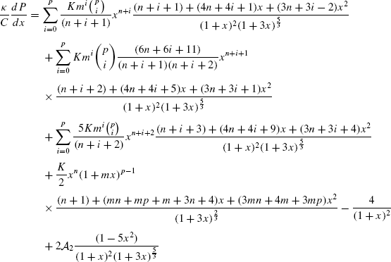
$$\begin{aligned} \frac{\kappa}{C} \frac{dP}{dx} =& K \sum_{i=0}^{p} {p\choose i} \frac{m^{i}}{ ( n+i+1 )} x^{n+i} \frac{ ( n+i+1 ) + ( 4n+4i+1 ) x+ ( 3n+3i-2 ) x^{2}}{ ( 1+x )^{2} ( 1+3x )^{\frac{5}{3}}} \\ &{}+5K \sum_{i=0}^{p} {p\choose i} \frac{m^{i}}{ ( n+i+1 )} x^{n+i+1} \\ &{}\times\frac{ ( n+i+2 ) + ( 4n+4i+5 ) x+ ( 3n+3i+1 ) x^{2}}{ ( 1+x )^{2} ( 1+3x )^{\frac{5}{3}}} \\ &{}+ \frac{K}{2} \frac{x^{n} ( 1+mx )^{p-1}}{( 1+x )^{2} ( 1+3x )^{\frac{2}{3}}} \bigl[( n+1 ) + ( mn+mp+m+4n+4 ) x\\ &{}+ ( 4mn+4mp+4m+3n+1) x^{2}+ ( 3mn+3mp+m ) x^{3}\bigr]\\ &{}-\frac{4}{ ( 1+x )^{2}} +2 \mathcal{A}_{2} \frac{ ( 1 - 5 x^{2} )}{ ( 1+x )^{2} ( 1+3x )^{\frac{5}{3}}} \end{aligned}$$$$\begin{aligned} \frac{\kappa}{C} \frac{d\rho}{dx} =& -K \sum_{i=0}^{p} {p\choose i} \frac{m^{i} ( 2n+2i+5 ) ( n+i+1 )}{ ( n+i+1 )} \frac{x^{n+i}}{ ( 1+3x )^{\frac{8}{3}}} \\ &{}-K \sum_{i=0}^{p} {p\choose i} \frac{m^{i} ( 2n+2i+5 ) ( 3n+3i-2 ) + ( 6n+6i+11 ) ( n+i+2 )}{ ( n+i+1 )} \\ &{}\times\frac{x^{n+i+1}}{ ( 1+3x )^{\frac{8}{3}}} \\ &{} -K \sum_{i=0}^{p} {p\choose i} \frac{m^{i} ( 6n+6i+11 ) ( 3n+3i+1 )}{ ( n+i+1 )} \frac{x^{n+i+2}}{ ( 1+3x )^{\frac{8}{3}}} \\ &{}- \frac{K}{2} \frac{x^{n} ( 1+mx )^{p-1}}{( 1+x )^{2} ( 1+3x )^{\frac{2}{3}}} \bigl[( n+1 ) + ( mn+mp+m+4n+4 ) x\\ &{}+ ( 4mn+4mp+4m+3n+1 ) x^{2}+ ( 3mn+3mp+m ) x^{3}\bigr]\\ &{}+10 \mathcal{A}_{2} \frac{ ( 1+x )}{ ( 1+3x )^{\frac{8}{3}}} \end{aligned}$$

5.2 Charge to Radius Ratio
From Eq. (2.9a)–(2.9c), using X=CR 2, we obtain the charge to radius ratio.
5.3 Mass to Radius Ratio (Compactness Parameter)
With the help of Eqs. (3.2b) and (3.3b) we can establish the equation of mass to radius ratio (compactness parameter).
5.4 Stellar Surface Density
Using X=CR 2 in the Eqs. (3.2e) and (3.3e) the equation of stellar surface density can be constructed as the following,


For the particular values of N, n, m, and p, the basic inputs to the above equations are K and X. In our study the values of parameters have been set in a way for which the energy density ρ, the pressure P and the electric charge Q remain positive and satisfy the necessary physical conditions.
For the numerical investigations the physical variables may be determined by three ways: for a given (i) radius, (ii) surface density, and (iii) central density. Only the case (ii) will be discussed. Thus for a given surface density, ρ s , in our model calculation we prefer ρ s =4.6888×10¹⁴ g cm−3 (paper I) the radius of the fluid sphere can be calculated by,
The maximum mass and corresponding radius of compact self-bound charged fluid spheres, obtained from the models considered, are reported in Table 2.
5.5 Discussions
The metric functions e ν and e λ are plotted in Figs. 1(a) and 1(b) respectively which show the continuity of those quantities. In Figs. 1(c) and 1(d) we have the behaviors of isotropic pressure and energy density which are positive and monotonically decreasing functions in the interior of the star. The pressure to density ratio, for fluid sphere obtained by assigning values of the parameters (p,m,n,K,X)=(1,−0.5,0.2,0.691,0.729), is presented in Fig. 1(e). The behaviors of the quantities \(\frac{\kappa}{C} \frac{dP}{dx},\ \frac{\kappa}{C} \frac{d\rho}{dx}\) are shown in Figs. 1(f)–1(g). It can be observed from the behavior of \(\sqrt{\frac{dP}{d\rho}}\), Fig. 1(h), that the speed of sound is always less than the speed of light and causality is maintained. The electric charge distribution for the same fluid sphere is plotted in Fig. 2, which is zero at the center and monotonically increasing towards the boundary. Figure 3 demonstrates the pressure-density relation.


Behaviors of (a) e ν, (b) e λ, (c) P (MeV fm−3), (d) ρ (MeV fm−3), (e) \(\frac{P}{\rho}\), (f) \(\frac{\kappa}{C} \frac{dP}{dx}\), (g) \(\frac{\kappa}{C} \frac{d \rho}{dx}\), (h) \(\sqrt{\frac{dP}{d\rho}}\) within fluid sphere described by the input (p,m,n,K,X)=(1,−0.5,0.2,0.691,0.729) using the charge distribution model II. The fractional radius \(( \frac{r}{R} )\) is plotted along the horizontal axis

Charge distribution within fluid sphere described by the same input as in Fig. 1. The fractional radius \(( \frac{r}{R} )\) and the charge Q (km) are plotted along the horizontal and vertical axes respectively

Pressure-density profile for fluid sphere described by the same input as in Fig. 1. The pressure P (MeV fm−3) and density ρ (MeV fm−3) are plotted along the horizontal and vertical axes respectively
The mass to radius ratio of charged fluid spheres are found to satisfy Böhmer–Harko limit [60], the lower limit of the allowable mass-to-radius ratio (M/R) for charged fluid sphere
Also the mass of the charged fluid sphere satisfies Andréasson [61] inequality, the charged analogue of Buchdahl inequality,
The mass-radius relation for the particular set of values (p,m,n,K)=(1,−0.5,0.2,0.691) and 0<X≤0.729, using model II, is graphed in Fig. 4. The behavior of Fig. 4 reproduces that of other quark star models (e.g., [12]).

Mass-radius relation for the input (p,m,n,K)=(1,−0.5,0.2,0.691) and 0≤X≤0.729 (model II). The radius R (km) and total mass M (in the unit of M ⊙) are plotted along the horizontal and vertical axes respectively
6 Conclusion
In this work some new families of exact solutions to the Einstein–Maxwell equations for a static spherically symmetric distribution of charged perfect fluid for particular forms of charge distribution were obtained and used to construct electrically charged self-bound stellar models. The relevant equations of state are also determined. These classes comprise some nonsingular stellar models, which have finite values for both the physical and metric variables at the stellar center. The method used in this paper to obtain new charged analogues to the neutral solutions depends crucially on the choice for the metric potential e ν and the forms electric charge distribution. It would be desirable to seek physically reasonable solutions, with new forms of e −λ.
The relationships between the total mass M, the total charge Q, and the constants \(\mathcal{B}_{N}\), C have been determined by the continuity of the metric coefficients across the boundary of the star to the unique exterior Reissner–Nordström solution. It has been showed that a wide range of charged spheres, with nonsingular potentials and matter variables, are possible for relevant choices of parameters.
References
Fatema, S., Murad, H.M.: An exact family of Einstein–Maxwell Wyman–Adler solution in general relativity. Int. J. Theor. Phys. (2013). doi:10.1007/s10773-013-1538-y
Patel, L.K., Pandya, B.M.: A Reissner–Nordström interior solution. Acta Phys. Hung., Heavy Ion Phys. 60, 57–65 (1986). doi:10.1007/BF03157418
Patel, L.K., Koppar, S.S.: A charged analogue of the Vaidya–Tikekar solution. Aust. J. Phys. 40, 441–447 (1987). doi:10.1071/PH870441
Koppar, S.S., Patel, L.K., Singh, T.: On relativistic charged fluid spheres. Acta Phys. Hung., Heavy Ion Phys. 69, 53–62 (1991). doi:10.1007/BF03054133
Patel, L.K., Tikekar, R., Sabu, M.C.: Exact interior solutions for charged fluid spheres. Gen. Relativ. Gravit. 29, 489–497 (1997). doi:10.1023/A:1018886816863
Sharma, R., Mukherjee, S., Maharaj, S.D.: General solution for a class of static charged spheres. Gen. Relativ. Gravit. 33, 999–1009 (2001). doi:10.1023/A:1010272130226
Komathiraj, K., Maharaj, S.D.: Tikekar superdense stars in electric fields. J. Math. Phys. 48, 042501 (2007). doi:10.1063/1.2716204
Lattimer, J.M., Prakash, M.: Neutron star structure and the equation of state. Astrophys. J. 550, 426–442 (2001). doi:10.1086/319702
Lattimer, J.M.: The structure of strange quark matter and neutron stars. J. Phys. G, Nucl. Part. Phys. 30, S479–S486 (2004). doi:10.1088/0954-3899/30/1/056
Lattimer, J.M., Prakash, M.: Ultimate energy density of observable cold baryonic matter. Phys. Rev. Lett. 94, 111101 (2005). doi:10.1103/PhysRevLett.94.111101
Delgaty, M.S.R., Lake, K.: Physical acceptability of isolated, static, spherically symmetric, perfect fluid solutions of Einstein’s equations. Comput. Phys. Commun. 115, 395–415 (1998). doi:10.1016/S0010-4655(98)00130-1
Negreiros, R.P., Weber, F., Malheiro, M., Vladimir, U.: Electrically charged strange quark stars. Phys. Rev. D 80, 083006 (2009). doi:10.1103/PhysRevD.80.083006
Komathiraj, K., Maharaj, S.D.: Analytical models of quark stars. Int. J. Mod. Phys. D 16, 1803–1811 (2011). doi:10.1142/S0218271807011103
Mak, M.K., Harko, T.: Quark stars admitting a one-parameter group of conformal motions. Int. J. Mod. Phys. D 13, 149–156 (2004). doi:10.1142/S0218271804004451
Rahaman, F., Sharma, R., Ray, S., Maulick, R., Karar, I.: Strange stars in Krori–Barua space-time. Eur. Phys. J. C 72, 2071 (2012). doi:10.1140/epjc/s10052-012-2071-5
Sharma, R., Karmakar, S., Mukherjee, S.: Maximum mass of a class of cold compact stars. Int. J. Mod. Phys. D 15, 405–418 (2006). doi:10.1142/S0218271806008012
Tikekar, R., Jotania, K.: On relativistic models of strange stars. Pramana J. Phys. 68, 397–406 (2007)
Chattopadhyay, P.K., Deb, R., Paul, B.C.: Relativistic solution for a class of static compact charged star in pseudo-spheroidal spacetime. Int. J. Mod. Phys. D 21, 1250071 (2012). doi:10.1142/S021827181250071X
Kalam, M., Usmani, A., Rahaman, F., Hossein, S.M., Karar, I., Sharma, R.: A relativistic model for strange quark stars. Int. J. Theor. Phys. (2012). doi:10.1007/s10773-013-1629-9
Durgapal, M.C.: A class of new exact solutions in general relativity. J. Phys. A, Math. Gen. 15, 2637–2644 (1982). doi:10.1088/0305-4470/15/8/039
Mak, M.K., Fung, P.C.W.: Charged static fluid spheres in general relativity. Nuovo Cimento B 110, 897–903 (1995). doi:10.1007/BF02722858
Mak, M.K., Fung, P.C.W., Harko, T.: New classes of interior solutions to Einstein–Maxwell equations in spherical symmetry. Nuovo Cimento B 111, 1461–1464 (1996). doi:10.1007/BF02741485
Ishak, M., Chamandy, L., Neary, N., Lake, K.: Exact solutions with w modes. Phys. Rev. D 64, 024005 (2001). doi:10.1103/PhysRevD.64.024005
Lake, K.: All static spherically symmetric perfect-fluid solutions of Einstein’s equations. Phys. Rev. D 67, 104015 (2003). doi:10.1103/PhysRevD.67.104015
Maurya, S.K., Gupta, Y.K.: On a family of well behaved perfect fluid balls as astrophysical objects in general relativity. Astrophys. Space Sci. 334, 145–154 (2011). doi:10.1007/s10509-011-0705-y
Tolman, R.C.: Static solutions of Einstein’s field equations for spheres of fluid. Phys. Rev. 55, 364–373 (1939). doi:10.1103/PhysRev.55.364
Pant, N., Rajasekhara, S.: Variety of well behaved parametric classes of relativistic charged fluid spheres in general relativity. Astrophys. Space Sci. 333, 161–168 (2011). doi:10.1007/s10509-011-0607-z
Pant, N., Negi, P.S.: Variety of well behaved exact solutions of Einstein–Maxwell field equations strange quark stars, neutron stars and pulsars. Astrophys. Space Sci. 338, 163–169 (2012). doi:10.1007/s10509-011-0919-z
Wyman, M.: Radially symmetric distribution of matter. Phys. Rev. 75, 1930–1936 (1949). doi:10.1103/PhysRev.75.1930
Adler, R.J.: A fluid sphere in general relativity. J. Math. Phys. 15, 727–729 (1974). doi:10.1063/1.1666717
Adams, R.C., Warburton, R.D., Cohen, J.M.: Analytic stellar models in general relativity. Astrophys. J. 200, 263–268 (1975). doi:10.1086/153627
Kuchowicz, B.: A physically realistic sphere of perfect fluid to serve as a model of neutron stars. Astrophys. Space Sci. 33, L13–L14 (1975). doi:10.1007/BF00646028
Pant, M.J., Tewari, B.C.: Well behaved class of charge analogue of Adler’s relativistic exact solution. J. Mod. Phys. 2, 481–487 (2011). doi:10.4236/jmp.2011.26058
Pant, N., Tewari, B.C., Fuloria, P.: Well behaved parametric class of exact solutions of Einstein–Maxwell field equations in general relativity. J. Mod. Phys. 2, 1538–1543 (2011). doi:10.4236/jmp.2011.212186
Pant, N., Faruqi, S.: Relativistic modeling of a superdense star containing a charged perfect fluid. Gravit. Cosmol. 18, 204–210 (2012). doi:10.1134/S0202289312030073
Murad, H.M.: A new well behaved class of charge analogue of Adler’s relativistic exact solution. Astrophys. Space Sci. 343, 187–194 (2013). doi:10.1007/s10509-012-1258-4
Heintzmann, H.: New exact static solutions of Einsteins field equations. Z. Phys. 228, 489–493 (1969). doi:10.1007/BF01558346
Korkina, M.P.: Static configuration with an ultrarelativistic equation of state at the center. Sov. Phys. J. 24, 468–470 (1981). doi:10.1007/BF00898413
Pant, N., Mehta, R.N., Pant, M.J.: Well behaved class of charge analogue of Heintzmann’s relativistic exact solution. Astrophys. Space Sci. 332, 473–479 (2011). doi:10.1007/s10509-010-0509-5
Pant, N., Maurya, S.K.: Relativistic modeling of charged super-dense star with Einstein–Maxwell equations in general relativity. Appl. Math. Comput. 218, 8260–8268 (2012). doi:10.1016/j.amc.2012.01.044
Pant, N.: Well behaved parametric class of relativistic charged fluid ball in general relativity. Astrophys. Space Sci. 332, 403–408 (2011). doi:10.1007/s10509-010-0521-9
Mehta, R.N., Pant, N., Mahto, D., Jha, J.S.: A well-behaved class of charged analogue of Durgapal solution. Astrophys. Space Sci. 343, 653–660 (2013). doi:10.1007/s10509-012-1289-x
Murad, H.M., Fatema, S.: A family of well behaved charge analogues of Durgapal’s perfect fluid exact solution in general relativity. Astrophys. Space Sci. 343, 587–597 (2013). doi:10.1007/s10509-012-1277-1
Maurya, S.K., Gupta, Y.K., Pratibha: Regular and well-behaved relativistic charged superdense star models. Int. J. Mod. Phys. D 20, 1289–1300 (2011). doi:10.1142/S0218271811019414
Faruqi, S., Pant, N.: Well-behaved relativistic charged super-dense star models. Astrophys. Space Sci. 341, 485–490 (2012). doi:10.1007/s10509-012-1132-4
Orlyansky, O.Y.: Singularity-free static fluid spheres in general relativity. J. Math. Phys. 38, 5301–5304 (1997). doi:10.1063/1.531943
Gupta, Y.K., Maurya, S.K.: A class of regular and well behaved relativistic super-dense star models. Astrophys. Space Sci. 332, 155–162 (2011). doi:10.1007/s10509-010-0503-y
Fuloria, P., Tewari, B.C., Joshi, B.C.: Well behaved class of charge analogue of Durgapal’s relativistic exact solution. J. Mod. Phys. 2, 1156–1160 (2011). doi:10.4236/jmp.2011.210143
Fuloria, P., Tewari, B.C.: A family of charge analogue of Durgapal solution. Astrophys. Space Sci. 341, 469–475 (2012). doi:10.1007/s10509-012-1105-7
Murad, H.M., Fatema, S.: A family of well behaved charge analogues of Durgapal’s perfect fluid exact solution in general relativity II. Astrophys. Space Sci. 344, 69–78 (2013). doi:10.1007/s10509-012-1320-2
Pant, N.: Some new exact solutions with finite central parameters and uniform radial motion of sound. Astrophys. Space Sci. 331, 633–644 (2011). doi:10.1007/s10509-010-0453-4
Maurya, S.K., Gupta, Y.K.: A family of well behaved charge analogues of a well behaved neutral solution in general relativity. Astrophys. Space Sci. 332, 481–490 (2011). doi:10.1007/s10509-010-0541-5
Pant, N.: New class of well behaved exact solutions of relativistic charged white-dwarf star with perfect fluid. Astrophys. Space Sci. 334, 267–271 (2011). doi:10.1007/s10509-011-0720-z
Pant, N.: New class of well behaved exact solutions for static charged neutron-star with perfect fluid. Astrophys. Space Sci. 337, 147–150 (2012). doi:10.1007/s10509-011-0809-4
Maurya, S.K., Gupta, Y.K., Pratibha: A class of charged relativistic superdense star models. Int. J. Theor. Phys. 51, 943–953 (2012). doi:10.1007/s10773-011-0968-7
Maurya, S.K., Gupta, Y.K.: Extremization of mass of charged superdense star models describe by Durgapal type space-time metric. Astrophys. Space Sci. 334, 301–310 (2011). doi:10.1007/s10509-011-0736-4
Maurya, S.K., Gupta, Y.K.: A new family of polynomial solutions for charged fluid spheres. Nonlinear Anal., Real World Appl. 13, 677–685 (2012). doi:10.1016/j.nonrwa.2011.08.008
Kuchowicz, B.: Differential conditions for physically meaningful fluid spheres in general relativity. Phys. Lett. A 38, 369–370 (1972). doi:10.1016/0375-9601(72)90164-8
Buchdahl, H.A.: Regular general relativistic charged fluid spheres. Acta Phys. Pol. B 10, 673–685 (1979)
Böhmer, C.G., Harko, T.: Minimum mass radius ratio for charged gravitational objects. Gen. Relativ. Gravit. 39, 757–775 (2007). doi:10.1007/s10714-007-0417-3
Andréasson, H.: Sharp bounds on the critical stability radius for relativistic charged spheres. Commun. Math. Phys. 288, 715–730 (2009). doi:10.1007/s00220-008-0690-3
Acknowledgements
Authors acknowledge their sincere gratitude to the reviewers for pointing out the errors and making relevant constructive suggestions that help authors improve the original manuscript.
Author information
Authors and Affiliations
Corresponding author
Additional information
This work is respectfully dedicated to the memory of our esteemed Professor J.N. Islam (1939–2013). With his death, we have lost a creative, thoughtful and an active member of the relativity-and-gravitation community.
Rights and permissions
About this article
Cite this article
Murad, M.H., Fatema, S. Some Exact Relativistic Models of Electrically Charged Self-bound Stars. Int J Theor Phys 52, 4342–4359 (2013). https://doi.org/10.1007/s10773-013-1752-7
Received:
Accepted:
Published:
Issue Date:
DOI: https://doi.org/10.1007/s10773-013-1752-7