
Abstract
In this paper, we have obtained a new singularity free charged anisotropic fluid solution of Einstein’s field equations. The physical parameters as radial pressure, tangential pressure, energy density, charge density, electric field intensity, velocity of sound and red-shift are well behaved everywhere inside the star. The obtained compact star models can represent the observational compact objects as PSR \(1937{+}21\) and PSR J1614–2230.
1 Introduction
Since the inception of Einstein field equation, the research workers are busy to obtain the compact star models such as neutron star and strange star models. To avoid the gravitational collapse, the presence of pressure with charge is more useful in averting the gravitational collapse by virtue of outward pressure with Columbian force. However the pressure anisotropy has also an important role to study of the compact stellar objects. Ruderman (1972) investigated about the realistic stellar models and conclude that the nuclear matter may be anisotropic at least very high density ranges of order more than \(10^{15}\ \mbox{gm/cm}^{3}\). Bowers and Liang (1974) have given the equation of state for relativistic anisotropic fluid sphere by generalizing the equation of hydrostatic equilibrium which include the effects the anisotropy. Recently Bhar and Ratanpal (2015) have obtained anisotropic star of Matese-Whitman Mass Function. Also Pant et al. (2016) obtained new charged anisotropic compact star models in isotropic coordinate system. In this connection Maurya et al. (2015a) developed the general algorithm for all spherically symmetric charged anisotropic solution. However the method for constructing the anisotropic factor by help of metric potential is given by Maurya et al. (2015b, 2015c). Also Maurya et al. (2015d, 2015e) have given the new approach to find the electromagnetic mass model in embedding class one metric. In similar fashion many workers have been obtained the anisotropic as well as charged anisotropic fluid solutions in different approaches (Dev and Gleiser 2002; Komathiraj and Maharaj 2007; Sunzu et al. 2014; Mak and Harko 2003; Mafa Takisa and Maharaj 2013, Maurya and Gupta 2012, 2013, 2014; Feroze and Siddiqui 2011; Pant et al. 2014, 2015; Malaver 2014, 2015; Esculpi et al. 2007; Herrera and Santos 1997; Herrera et al. 2004, 2008; Cosenza et al. 1981; Gokhroo and Mehra 1994; Maurya et al. 2015f, 2016).
In the present article we have obtained the new model for charged anisotropic solution. For this purpose we have started the metric potential of the form \(e^{\lambda} = \frac{1 + ar^{2}}{1 - br^{2}}\). The structure of the paper as follows: Sect. 2 contains the Einstein field equations for charged anisotropic sphere. In Sect. 3: we determine the mass function by considering the electric intensity (\(E = \frac{q}{r^{2}}\)) and metric potential \(e^{\lambda}\) after that we obtained the metric function \(\nu\) by taking physically valid expression of radial pressure. However the anisotropy factor is determined by using the pressure isotropy condition. In Sect. 4: we join the metric to Reissner-Nordstrom metric at the surface of the star and obtained the arbitrary constants. However the physical features of charged anisotropic models are given in Sect. 5. Section 6 is containing the stability analysis, amount of the charge and surface red-shift of the compact stars. We presented the maximum allowable mass to radius ratio and validity of strange star candidates in Sect. 7. At last the conclusion of the article is given in Sect. 8.
2 The Einstein’s field equation for charged anisotropic fluid distributions
Let us consider a static spherically symmetric metric for charged anisotropic matter distribution as:
The Einstein-Maxwell field equations are given by
where \(\kappa = 8\pi\) is the Einstein constant with \(G = 1 = c\) in relativistic geometrized unit. However \(G\) and \(c\) respectively being the Newtonian gravitational constant and velocity of photon in vacuum.
We assumed that the matter inside the star is to be locally anisotropic fluid. So the energy momentum tensor (\(T_{j}^{i}\)) and electromagnetic tensor (\(E_{j}^{i}\)) are defined by (Dionysiou 1982):
where \(\theta^{i}\) is the unit space like vector in the direction of radial vector as \(\theta^{i} = e^{\lambda (r)/2} \delta_{1}^{i}\), \(v^{i}\) is the four-velocity as \(e^{\lambda (r)/2}v^{i} = \delta_{4}^{i}\), \(p_{r}\) is the pressure in direction of \(\theta^{i}\) (normal pressure) and \(p_{t}\) is the pressure orthogonal to \(\theta_{i}\) (transversal or tangential pressure) and \(\rho\) is the energy density.
For the spherically symmetric metric (1), the Einstein-Maxwell field equations may be expressed as the following system of ordinary differential equations (Dionysiou 1982):
where the prime denotes differential with respect to ‘\(r\)’ and \(E = \frac{1}{r^{2}}\int_{0}^{r} 4\pi r^{2}\sigma e^{\lambda /2} = \frac{q}{r^{2}}\). However \(\sigma\) is the charge density.
3 New charged anisotropic solution for compact star
The mass function \(m(r)\) for electrically charged fluid sphere can be defined in terms of metric function \(e^{\lambda (r)}\) as:
To determine the mass function \(m(r)\), we consider the metric potential \(e^{\lambda (r)}\) and electric intensity \(E\) of the form:
where \(a\), \(b\) and \(E_{0}\) are positive constants.
We observe from Eq. (10), the electric intensity is zero at the centre and monotonically increasing away from the centre. However the charge density is singularity free at the centre and monotonically decreasing. The behavior can be seen in Fig. 1.

Behavior of electric intensity (\(E^{2}\)) and charge density (\(\sigma\)) with respect to radial coordinate \(r/R\). We have used the numerical values of the parameters in this figure as: (i) \(a=0.00774\), \(b=0.0001\), \(p_{0} =0.0028\), \(E_{0} =0.0001\) for PSR J1614–2230, (ii) \(a=0.007562\), \(b=0.00053\), \(p_{0} =0.0035\), \(E_{0} =0.0008\) for PSR \(1937{+}21\)
By plugging Eq. (9) and Eq. (10) into Eq. (8), we get:
However from Eq. (5) and Eq. (6), corresponding the matter density (\(\rho\)) and metric function (\(\nu\)) are given as:
To integrate Eq. (13), we suppose the radial pressure of the form:
where \(p_{0}\) is positive constant and the expression of \(p_{r}\) is physically valid as it is positive, finite and monotonically decreasing function with increase of ‘\(r\)’. However it vanish at \(r = \frac{1}{\sqrt{a}}\), which gives the radius of the star.
After putting the value of \(p_{r}\) in Eq. (13), we get:
After integration, we get the metric function (\(\nu\)) of the form:
where
and \(C\) is arbitrary positive constants of integration.
Now the expression for anisotropy factor \(\Delta = p_{t} - p_{r}\) can be determined by using the pressure isotropy condition as:
where
4 Matching conditions
We join smoothly the interior of metric (1) to an exterior Reissner-Nordstrom metric:
at the surface of spheres (\(r = R\)). This requires the continuity of the components \(g_{i j}\) at \(r = R\). However the requirements of matching condition for metric (1) that the above system of equations is to be solved subject to the boundary condition that radial pressure \(p_{r} = 0\) at \(r = R\), whose mass is same as \(m (r = R) = M\) (Misner and Sharp 1964).
These conditions are as follows:
where \(M\) and \(Q\) are called the total mass and charge inside the fluid sphere respectively. The conditions (19) and (21) gives respectively:
and
5 Physical features of the charged anisotropic models
(i) For physical acceptable charged anisotropic models, the metric potentials \(e^{\lambda (r)}\) and \(e^{\nu (r)}\)should have non-zero positive values in the range \(0 \le r \le R\) and free from singularity at \(r = 0\). At the origin Eqs. (9) and (16) provides \(e^{\lambda (0)} = 1\) and \(e^{\nu (0)} = C\). So it is clear that metric potentials are positive and finite at the centre of star (Fig. 4).
(ii) The radial pressure (\(p_{r}\)), tangential pressure (\(p_{t}\)), energy density (\(\rho\)) should be finite at the centre \(r = 0\) and monotonically decreasing throughout inside the star. These behaviors can be seen in Figs. 2 and 5.

Behavior of matter-energy density (\(\rho\)) with respect to radial coordinate \(r/R\). For purpose of plotting this graph, we have employed the data set of values in this figure same as used in Fig. 1
(iii) Inside the fluid sphere, the speed of sound should be less than the speed of light, i.e., \(0 \le V_{r} = \sqrt{dp_{r}/d\rho} < 1\) and \(0 \le V_{t} = \sqrt{dp_{t}/d\rho} < 1\). However for well behaved nature of the solution, both velocities should be monotonically decreasing away from the centre to boundary of the sphere which can be observed from Fig. 6.
6 Stability analysis, electric charge, charge density and red-shift
6.1 Stability analysis
To verify the stability of our charged anisotropic models, we plot the square of radial speed of sound (\(V_{r}^{2}\)) and transverse speed of sound (\(V_{t}^{2}\)) in Fig. 7. As we note from Fig. 7 that both of these parameters satisfy the inequalities \(0 \le V_{r}^{2} < 1\) and \(0 \le V_{t}^{2} < 1\) everywhere inside the star.
Now to determine the charged anisotropic matter distribution is stable or not, for this we will use Herrera (1992), cracking (or overturning) concept, which states that the potentially stable region is that one where radial speed of sound is greater than the transverse speed of sound. This implies that there is no change in sign of \(V_{r}^{2}\)–\(V_{t}^{2}\) and \(V_{t}^{2}\)–\(V_{r}^{2}\). This can be seen from Fig. 8 that there is no change in sign of above both conditions. So, it is clear that our models are stable.
6.2 Electric charge and charge density
We observed that the electric charge on the boundary, in the unit of Coulomb, is \(7.5317 \times 10^{19}\) Coulomb for PSR J1664–2230 and \(9.8951 \times 10^{19}\) Coulomb for PSR \(1937+21\) and at the centre both are as usual zero. In Table 1 we have put the data for charge \(q\) in the relativistic unit km. However, to convert these values in Coulomb one has to multiply every value by a factor \(1.1659 \times 10^{20}\). The graphical plot is shown in Fig. 1 where charge profile is such that starting from a minimum and it acquires maximum value at the boundary. However the charge density is maximum at center and monotonically decreasing outward. The plot for charge density is given in Fig. 1 and numerical values in Table 1.
6.3 Surface red-shift
The effective gravitational mass in terms of the energy density can be written as
where \(e^{ - \lambda (R)}\) is given by Eq. (9).
Therefore the compactness of the star can be defined as:
Now we define the surface red-shift for charged compact star corresponding to the above compactness factor \((u)\) as follows:
We plot Fig. 9 for surface red-shift and observe that it is decreasing away from the centre. The maximum surface red-shift attains at the centre and minimum at boundary. The corresponding values are: (i) at centre: \(Z_{0} = 0.9003\) for PSR J164–2230 and \(Z_{0} = 1.0239\) for PSR \(1937{+}21\), (ii) at surface: \(Z_{R} = 0.4234\) for PSR J164–2230 and \(Z_{R} = 0.4664\) for PSR \(1937{+}21\). In this connection, in absence of the cosmological constant the surface red-shift has constraint as \(Z \le 2\) (Buchdahl 1959; Straumann 1984; Bohmer and Harko 2006) for the isotropic case. However for an anisotropic star in the presence of a cosmological constant the constraint on surface redshift is \(Z \le 5\) (Bohmer and Harko 2006) whereas Ivanov (2002) has put the bound \(Z \le 5.211\). Based on the above discussion we therefore conclude that for an anisotropic star without cosmological constant the values for our models \(Z = 0.9003\) and \(Z = 1.0239\) are in good agreement.
7 Mass-radius ratio and validity with strange star candidates
7.1 Maximum allowable mass to radius ratio
The maximum mass for compact star cannot be arbitrary large. Buchdahl (1959) has given an absolute constraint of the maximally allowable mass-to-radius ratio \((M/R)\) for isotropic fluid spheres of the form \(2M/R \le 8/9\) (in the unit, \(c = G = 1\)), which states that, for a given radius a static isotropic fluid sphere cannot be arbitrarily massive. However Bohmer and Harko (2007) provided the lower bound for the mass-radius ratio for a compact object with charge, \(Q\) (\(< M\)), as:
Also, Andreasson (2009) has generalized the mass-radius ratio for charged compact star and prove that upper bound of the mass satisfy the inequality:
After combining both of above inequalities, we get:
7.2 Validity with strange star candidates
As proposed Tables 2 and 3, it is clear that the mass and radius are exactly corresponding to the compact stars RXJ1856–37 and PSR \(1937+21\). The details of the tables are as follows: we consider the mass and radius of the above mentioned stars and determine the data for the model parameters. In the next step we have calculated the data values for different physical parameters like central density, surface density and central pressure, of those compact stars. We can observe that these physical data sets are in good agreement with the available observational data.
8 Conclusions
In the present article, we have proposed new model for charged anisotropic compact stars PSR \(1937{+}21\) and PSR J1664–2230. For this purpose we started with the metric potential \(e^{\lambda} = \frac{1 + ar^{2}}{1 - br^{2}}\) and electric intensity \(E = \frac{r\sqrt{E_{0} a}}{(1 + ar^{2})}\). After that we determine the mass function \(m (r)\). It is clear from Eq. (18), the mass is zero at the centre and free from singularity everywhere inside the star. Now our next aim to find the metric potential ‘\(\nu \)’. We suppose the radial pressure \(p_{r}\) of the form \(p_{r} = \frac{p_{0} (1 - a r^{2})}{8 \pi (1 + a r^{2})^{2}}\) which is finite at the centre and zero at \(r = \frac{1}{\sqrt{a}}\). The obtained metric function ‘\(\nu \)’ is given by Eq. (16). However the pressure anisotropy factor ‘\(\Delta \)’ has been determined by using the pressure isotropy condition. This ‘\(\Delta \)’ is also zero at centre and monotonic increasing with increase of ‘\(r \)’ (Fig. 3). In Sect. 4, we obtained arbitrary constants by using the boundary conditions.

The physical features of the models as follows:
-
(i)
The behavior of metric potentials are given by Fig. 4, from this figure it is clear that metric potentials are free from singularity and finite everywhere inside the star.
Fig. 4 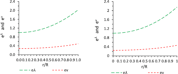
Behavior of metric potentials \(e^{\lambda}\) and \(e^{\nu}\) for PSR J1614–2030 (left panel) and PSR \(1937{+}21\) (right panel) with respect to radial coordinate \(r/R\). We have used the numerical values of the parameters in this figure as: (i) \(a=0.00774\), \(b=0.0001\), \(p_{0} =0.0028\), \(E_{0} =0.0001\) for PSR J1614–2230, (ii) \(\mathrm{a}=0.007562\), \(b=0.00053\), \(p_{0} =0.0035\), \(E_{0} =0.0008\) for PSR \(1937{+}21\)
Fig. 5 
Behavior of radial and tangential pressures \(p_{r}\) (left panel) and \(p_{t}\) (right panel) with respect to radial coordinate \(r = R\). For purpose of plotting this graph, we have employed the data set of values in this figure same as used in Fig. 4
-
(ii)
The plot for electric charge \((E)\) and energy density (\(\rho\)) are shown in Figs. 1 and 2 respectively. From these figures, we observe that the electric charge is zero at centre and monotonically increasing away from the centre. However the energy density is monotonically decreasing away from the centre.
-
(iii)
Inside the fluid sphere, the speed of sound is less the speed of light, i.e. our charged anisotropic models are well behaved (the plot for this feature can be seen from Fig. 6).
Fig. 6 
Behavior of sound speed \(V_{r}\) (left panel) and \(V_{t}\) (right panel) with respect to radial coordinate \(r = R\). We have used the numerical values of the parameters in this figure as: (i) \(a=0.00774\), \(b=0.0001\), \(p_{0} =0.0028\), \(E_{0} =0.0001\) for PSR J1614–2230, (ii) \(a=0.007562\), \(b=0.00053\), \(p_{0} =0.0035\), \(E_{0} =0.0008\) for PSR \(1937{+}21\)
-
(iv)
Section 6 contains the stability analysis, electric charge and red-shift of the compact star models. To verify the stability of the models we determine the square of radial and tangential velocity of sound (Fig. 7). From Fig. 7, we note that it is lies between 0 and 1. After that we used Herrera (1992) cracking concept, for this purpose we calculate the difference \(V_{r}^{2}\)–\(V_{t}^{2}\) and \(V_{t}^{2}\)–\(V_{r}^{2}\). As we can see from Fig. 8, there is no change in sign of \(V_{r}^{2} \)–\(V_{t}^{2}\)and \(V_{t}^{2} \)–\(V_{r}^{2}\). So our models are stable. However the amount of charge of the compact star PSR \(1937{+}21\) and PSR J1664–2230 are shown in Table 1.
Fig. 7 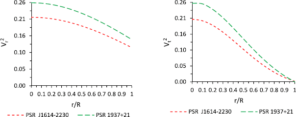
Behavior of the square of the sound speed \(V_{r}^{2}\) and \(V_{t}^{2}\) with respect to radial coordinate \(r/R\). For purpose of plotting this graph, we have employed the data set of values in this figure same as used in Fig. 6
-
(v)
We plotted the behavior of red shift in Fig. 9, which shows that it is maximum at centre and monotonic decreasing with increase of radius ‘\(r \)’. The Maximum allowable mass–radius ratio for PSR \(1937{+}21\) and PSR J1664–2230 are given in Table 2.
Fig. 9 
Behavior of red-shift of the charged anisotropic model with respect to radial coordinate \(r/R\). The date values used in this figure as: (i) \(a=0.00774\), \(b=0.0001\), \(p_{0} =0.0028\), \(E_{0} =0.0001\) for PSR J1614–2230, (ii) \(a=0.007562\), \(b=0.00053\), \(p_{0} =0.0035\), \(E_{0} =0.0008\) for PSR \(1937{+}21\)


Where the various symbols used in the figures and tables stand for the following physical entities
\(Z_{0}= \text{red}\) shift at the centre, \(Z_{R}= \text{red}\) shift at the surface, Solar mass \(M_{\Theta} =1.475\ \mbox{km}\), \(G = 6.673 \times 10^{ - 8}\ \mbox{cm}^{3}/\mbox{gs}^{2}\), \(c = 2.997 \times 10^{10}\ \mbox{cm}/\mbox{s}\).
References
Andreasson, H.: Commun. Math. Phys. 288, 715 (2009)
Bhar, P., Ratanpal, B.S.: arXiv:1511.06962v1 [gr-qc] (2015)
Bohmer, C.G., Harko, T.: Class. Quantum Gravity 23, 6479 (2006)
Bohmer, C.G., Harko, T.: Gen. Relativ. Gravit. 39, 757 (2007)
Bowers, R., Liang, E.: Astrophys. J. 188, 657 (1974)
Buchdahl, H.A.: Phys. Rev. 116, 1027 (1959)
Cosenza, M., Herrera, L., Esculpi, M., Witten, L.: J. Math. Phys. 22(1), 118 (1981)
Dev, K., Gleiser, M.: Gen. Relativ. Gravit. 34, 1793 (2002)
Dionysiou, D.D.: Astrophys. Space Sci. 85, 331 (1982)
Esculpi, M., Malaver, M., Aloma, E.: Gen. Relativ. Gravit. 39, 633 (2007)
Feroze, T., Siddiqui, A.A.: Gen. Relativ. Gravit. 43, 1025 (2011)
Gokhroo, M.K., Mehra, A.L.: Gen. Relativ. Gravit. 26(1), 75–84 (1994)
Herrera, L.: Phys. Lett. A 165, 206 (1992)
Herrera, L., Santos, N.O.: Phys. Rep. 53, 286 (1997)
Herrera, L., et al.: Phys. Rev. D 69, 084026 (2004)
Herrera, L., Santos, N.O., Wang, A.: Phys. Rev. D 78, 084026 (2008)
Ivanov, B.V.: Phys. Rev. D 65, 104001 (2002)
Komathiraj, K., Maharaj, S.D.: J. Math. Phys. 48, 042501 (2007)
Mafa Takisa, P., Maharaj, S.D.: Gen. Relativ. Gravit. 45, 1951–1969 (2013)
Mak, M.K., Harko, T.: Proc. R. Soc. A 459, 393 (2003)
Malaver, M.: Front. Math. Appl. 1, 9 (2014)
Malaver, M.: Int. J. Mod. Phys. Appl. 2(1), 1–6 (2015). arXiv:1503.06678
Maurya, S.K., Gupta, Y.K.: Phys. Scr. 86, 025009 (2012)
Maurya, S.K., Gupta, Y.K.: Astrophys. Space Sci. 344, 243 (2013)
Maurya, S.K., Gupta, Y.K.: Astrophys. Space Sci. 353, 657 (2014)
Maurya, S.K., Gupta, Y.K., Ray, S.:. arXiv:1502.01915 [gr-qc] (2015a)
Maurya, S.K., Gupta, Y.K., Ray, S., Dayanandan, B.: Eur. Phys. J. C 75, 225 (2015b)
Maurya, S.K., Gupta, Y.K., Dayanandan, B., Jasim, M.K., Al Jamel, A.: arXiv:1511.01625 [gr-qc] (2015c)
Maurya, S.K., Gupta, Y.K., Ray, S., Chowdhury, S.R.: Eur. Phys. J. C 75, 389 (2015d)
Maurya, S.K., Gupta, Y.K., Ray, S., Chatterjee, V.: arXiv:1507.01862 [gr-qc] (2015e)
Maurya, S.K., Smitha, T.T., Gupta, Y.K., Rahaman, F.: arXiv:1512.01667 [gr-qc] (2015f)
Maurya, S.K., Gupta, Y.K., Dayanandan, B., Ray, S.: arXiv:1512.09350 (2016)
Misner, C.W., Sharp, D.H.: Phys. Rev. B 136, 571 (1964)
Pant, N., Pradhan, N., Singh, N.K.: J. Gravity 380, 320 (2014)
Pant, N., Pardhan, N., Malaver, M.: Int. J. Astrophys. Space Sci. 3, 1–5 (2015)
Pant, N., Pradhan, N., Bansal, R.K.: Astrophys. Space Sci. 361, 41 (2016)
Ruderman, R.: Annu. Rev. Astron. Astrophys. 10, 427 (1972)
Straumann, N.: General Relativity and Relativistic Astrophysics. Springer, Berlin (1984)
Sunzu, M.J., Maharaj, S.D., Ray, S.: Astrophys. Space Sci. 352, 719–727 (2014)
Acknowledgements
The authors acknowledge that this research work is supported by research project of University of Nizwa, Nizwa, Sultanate of Oman. Also we are highly obliged to the referees for their valuable comments and suggestions.
Author information
Authors and Affiliations
Corresponding author
Rights and permissions
About this article

Cite this article
Maurya, S.K., Jasim, M.K., Gupta, Y.K. et al. A new model for charged anisotropic compact star. Astrophys Space Sci 361, 163 (2016). https://doi.org/10.1007/s10509-016-2747-7
Received:
Accepted:
Published:
DOI: https://doi.org/10.1007/s10509-016-2747-7