Multi-circle detection on images inspired by collective animal behavior

Abstract

Hough transform (HT) has been the most common method for circle detection that delivers robustness but adversely demands considerable computational efforts and large memory requirements. As an alternative to HT-based techniques, the problem of shape recognition has also been handled through optimization methods. In particular, extracting multiple circle primitives falls into the category of multi-modal optimization as each circle represents an optimum which must be detected within the feasible solution space. However, since all optimization-based circle detectors focus on finding only a single optimal solution, they need to be applied several times in order to extract all the primitives which results on time-consuming algorithms. This paper presents an algorithm for automatic detection of multiple circular shapes that considers the overall process as a multi-modal optimization problem. In the detection, the approach employs an evolutionary algorithm based on the way in which the animals behave collectively. In such an algorithm, searcher agents emulate a group of animals which interact to each other using simple biological rules. These rules are modeled as evolutionary operators. Such operators are applied to each agent considering that the complete group maintains a memory which stores the optimal solutions seen so-far by applying a competition principle. The detector uses a combination of three non-collinear edge points as parameters to determine circle candidates (possible solutions). A matching function determines if such circle candidates are actually present in the image. Guided by the values of such matching functions, the set of encoded candidate circles are evolved through the evolutionary algorithm so that the best candidate (global optimum) can be fitted into an actual circle within the edge-only image. Subsequently, an analysis of the incorporated memory is executed in order to identify potential local optima which represent other circles. Experimental results over several complex synthetic and natural images have validated the efficiency of the proposed technique regarding accuracy, speed and robustness.

1 Introduction

The problem of detecting circular features holds paramount importance for image analysis in industrial applications such as automatic inspection of manufactured products and components, aided vectorization of drawings, target detection, etc. [1]. In the last decade, the detection accuracy and computation performance are two main concerned issues and many circle detection methods have been developed.

The circle detection in digital images is commonly solved through the Circular Hough Transform (CHT) [2]. A typical Hough-based approach employs an edge detector and some edge information to infer locations and radii values. Peak detection is then performed by averaging, filtering and histogramming within the transform space. Unfortunately, such an approach requires a large storage space as the 3-D cells include parameters (x,y,r) that augment the computational complexity and yield a low processing speed. The accuracy of parameters for the extracted circles is poor, particularly under noisy conditions [2]. In the particular case of a digital image holding a significant width and height, and some densely populated edge pixels, the required processing time for Circular Hough Transform makes it prohibitive to be deployed in several applications. In order to overcome such a problem, some other researchers have proposed new approaches following Hough transform principles, yielding the probabilistic Hough transform [3], the randomized Hough transform (RHT) [4], the fuzzy Hough transform [5] and some other methods discussed by Becker in [6]. All these approaches significantly reduce the computational effort and memory requirements in comparison to the original CHT. However, they notoriously fail while dealing with images contaminated with noise (despite very low levels) or with circles which are not well defined (occluded or overlapped) [7].

As an alternative to Hough Transform-based techniques, the problem of shape recognition has also been handled through optimization methods [8, 9]. In general, they have demonstrated to deliver better results than those based on the HT considering accuracy, speed and robustness [10]. Such approaches have produced several robust circle detectors using different optimization algorithms such as Genetic algorithms (GA) [10], Harmony Search (HSA) [11], Electromagnetism-Like (EMO) [12], Differential Evolution (DE) [13] and Bacterial Foraging Optimization (BFOA) [14]. Since such evolutionary algorithms are global optimizers, they detect only the global optimum of an objective function that is defined over a given search space [15]. Considering such fact, all these optimization-based detectors work in the original edge image until the convergence for the first circle recognition is achieved (global optimum). Such shape is then eliminated from the edge-only image and the optimization method is executed again over the modified image. The procedure is repeated until the maximum number of circles is attained (all important optima are found). Under such circumstances, these approaches produce circle detectors which demand considerable time resources in order to accomplish their goal.

In contrast to global optimization, the multi-modal optimization approach [16] delivers the detection of multiple global and local optima of a given objective function. Extracting multiple circle primitives falls into the category of multi-modal optimization, where each circle represents an optimum which must be detected within a feasible solution space. The quality for such optima is characterized by the properties of their geometric primitives. Big and well drawn circles normally represent points in the search space with high fitness values (possible global maximum) whereas small and dashed circles describe points with fitness values which account for local maxima. Likewise, circles holding similar geometric properties, such as radius, size, etc., tend to represent locations with similar fitness values.

Therefore, a multi-modal method must be applied in order to appropriately solve the problem of multi-shape detection. Several multi-modal optimization algorithms are based on a large variety of different techniques that have been proposed in the literature. Among them, ‘niches and species’ and a fitness sharing method [17] have been introduced to overcome the weakness of traditional evolutionary algorithms for multimodal optimization. In this work, a new optimization algorithm based on the collective animal behavior to solve multimodal problems is applied to multi-circle detection.

Several studies, which have been inspired by animal behavior phenomena, have been applied to develop optimization techniques such as the Particle swarm optimization (PSO) that models the social behavior of bird flocking or fish schooling [18]. In a PSO process, a swarm of particles (or agents), each of which represents a potential solution to an optimization problem, sweeps through the search space. Each particle registers its position within the search space and the best solution achieved so far. This is best particle’s value and the PSO process also keeps track of the global best solution achieved so far by the swarm and its correspondent particle index. Therefore, during their evolution, the position of each agent in the next iteration is modified yielding an attraction movement towards the best position of the swarm and the best particle’s position [19, 20]. In recent years, there have been several attempts to apply the PSO to multi-modal function optimization problems [21, 22]. However, the performance of such approaches presents several flaws when it is compared to other multi-modal metaheuristic counterparts [23].

Recently, the concept of individual-organization [24, 25] has been widely used to understand collective behavior of animals. The central principle of individual-organization is that simple repeated interactions between individuals can produce complex behavioral patterns at group level [24, 26, 27]. Such inspiration comes from behavioral patterns seen in several animal groups, such as ant pheromone trail networks, aggregation of cockroaches and the migration of fish schools, which can be accurately described in terms of individuals following simple sets of rules [28]. Some examples of these rules [27, 29] include keeping current position (or location) for best individuals, local attraction or repulsion, random movements and competition for the space inside of a determined distance. On the other hand, new studies have also shown the existence of collective memory in animal groups [30–32]. The presence of such memory establishes that the previous history, of group structure, influences the collective behavior exhibited in future stages. Therefore, according to these new developments, it is possible to model complex collective behaviors by using simple individual rules and configuring a general memory.

This paper presents an algorithm for automatic detection of multiple circular shapes that considers the overall process as a multi-modal optimization problem. In the detection, the approach employs an evolutionary algorithm based on the way animals behave collectively. In such algorithm, searcher agents emulate a group of animals that interact to each other by simple biological rules which are modeled as evolution operators. Such operators are applied to each agent considering that the complete group has a memory which stores the optimal solutions seen so-far by applying a competition principle. In contrast to PSO, the proposed scheme modifies some evolution operators for allowing not only attracting, but also repelling movements among particles. Likewise, instead of simply choosing the best position as reference, our algorithm uses a set of neighboring elements that are contained in a incorporated memory. Such improvements increase the algorithm’s capacity to explore and to exploit the set of solutions which are operated during the evolving process.

The proposed detector uses a combination of three non-collinear edge points as parameters to determine circle candidates (possible solutions). A matching function determines if such circle candidates are actually present in the image. Guided by the values of such matching functions, the set of encoded candidate circles are evolved through the evolutionary algorithm so that the best candidate can be fitted into the actual circle within the image. Then, an analysis of the incorporated memory is executed in order to identify potential local optima, i.e., other circles. Experimental results over several complex synthetic and natural images have validated the efficiency of the proposed technique regarding accuracy, speed and robustness.

The paper is organized as follows: Sect. 2 provides information regarding the evolutionary algorithm based on the way animals behave collectively (CAB). Section 3 depicts the implementation of the proposed circle detector. The complete multiple circle detection procedure is presented by Sect. 4. Experimental results for the proposed approach are stated in Sect. 5 and some relevant conclusions are discussed in Sect. 6.

2 Collective Animal Behavior algorithm (CAB)

The CAB algorithm assumes the existence of a set of operations that resembles the interaction rules that model the collective animal behavior. In the approach, each solution within the search space represents an animal position. The “fitness value” refers to the animal dominance with respect to the group. The complete process mimics the collective animal behavior.

The approach in this paper implements memory for storing best solutions (animal positions) mimicking the aforementioned biologic process. Such memory is divided into two different elements, one for maintaining the best locations at each generation (M _g ) and the other for storing the best historical positions during the complete evolutionary process (M _h ).

2.1 Description of the CAB algorithm

Following other metaheuristic approaches, the CAB algorithm is an iterative process that starts by initializing the population randomly (generated random solutions or animal positions). Then, the following four operations are applied until a termination criterion is met (i.e. the iteration number NI):

• 1. Keep the position of the best individuals.

• 2. Move from or to nearby neighbors (local attraction and repulsion).

• 3. Move randomly.

• 4. Compete for the space within a determined distance (update the memory).

2.1.1 Initializing the population

The algorithm begins by initializing a set A of N _p animal positions ($\mathbf{A} = \{ \mathbf{a}_{1},\mathbf{a}_{2}, \ldots,\mathbf{a}_{N_{p}}\}$). Each animal position a _i is a D-dimensional vector containing parameter values to be optimized. Such values are randomly and uniformly distributed between the pre-specified lower initial parameter bound $a_{j}^{\mathit{low}}$ and the upper initial parameter bound $a_{j}^{\mathit{high}}$.

(1)

with j and i being the parameter and individual indexes respectively. Hence, a _j,i is the jth parameter of the ith individual.

All the initial positions A are sorted according to the fitness function (dominance) to form a new individual set $\mathbf{X} = \{ \mathbf{x}_{1},\mathbf{x}_{2}, \ldots,\mathbf{x}_{N_{p}}\}$, so that we can choose the best B positions and store them in the memory M _g and M _h . The fact that both memories share the same information is only allowed at this initial stage.

2.1.2 Keep the position of the best individuals

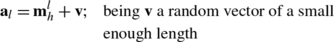
Analogous to the biological metaphor, this behavioral rule, typical from animal groups, is implemented as an evolutionary operation in our approach. In this operation, the first B elements ({a ₁,a ₂,…,a _B }), of the new animal position set A, are generated. Such positions are computed by the values contained inside the historical memory M _h , considering a slight random perturbation around them. This operation can be modeled as follows:

(2)

where l∈{1,2,…,B} while $\mathbf{m}_{h}^{l}$ represents the l-element of the historical memory M _h .v is a random vector with a small enough length.

2.1.3 Move from or to nearby neighbors

From the biological inspiration, animals experiment a random local attraction or repulsion according to an internal motivation. Therefore, we have implemented new evolutionary operators that mimic such biological pattern. For this operation, a uniform random number r _m is generated within the range [0,1]. If r _m is less than a threshold H, a determined individual position is moved (attracted or repelled) considering the nearest best historical position within the group (i.e. the nearest position in M _h ); otherwise, it goes to the nearest best location within the group for the current generation (i.e. the nearest position in M _g ). Therefore such operation can be modeled as follows:

(3)

where i∈{B+1,B+2,…,N _p }, $\mathbf{m}_{h}^{\mathit{nearest}}$ and $\mathbf{m}_{g}^{\mathit{nearest}}$ represent the nearest elements of M _h and M _g to x _i , while r is a random number between [−1,1]. Therefore, if r>0, the individual position x _i is attracted to the position $\mathbf{m}_{h}^{\mathit{nearest}}$ or $\mathbf{m}_{g}^{\mathit{nearest}}$, otherwise such movement is considered as a repulsion.

2.1.4 Move randomly

Following the biological model, under some probability P, one animal randomly changes its position. Such behavioral rule is implemented considering the next expression:

(4)

with i∈{B+1,B+2,…,N _p } and r a random vector defined in the search space. This operator is similar to re-initialize the particle in a random position, as it is done by Eq. (1).

2.1.5 Compete for the space within of a determined distance (update the memory)

Once the operations to keep the position of the best individuals, such as moving from or to nearby neighbors and moving randomly, have all been applied to the all N _p animal positions, it is necessary to update the memory M _h .

In order to update the memory M _h , the concept of dominance is used. Animals that interact within a group maintain a minimum distance among them. Such distance ρ depends on how aggressive the animal behaves [33, 34]. Hence, when two animals confront each other inside such distance, the most dominant individual prevails while the other withdraws. Figure 1 depicts the process.

Fig. 1

Dominance concept as it is presented when two animals confront each other inside of a ρ distance

In the proposed algorithm, the historical memory M _h is updated considering the following procedure:

• 1. The elements of M _h and M _g are merged into M _U (M _U =M _h ∪M _g ).

• 2. Each element $\mathbf{m}_{U}^{i}$ of the memory M _U is compared pair-wise to remaining memory elements ($\{ \mathbf{m}_{U}^{1},\mathbf{m}_{U}^{2}, \ldots,\mathbf{m}_{U}^{2B - 1} \}$). If the distance between both elements is less than ρ, the element getting a better performance in the fitness function prevails meanwhile the other is removed.

• 3. From the resulting elements of M _U (from step 2), it is selected the B best value to build the new M _h .

The use of the dominance principle in CAB allows considering as memory elements those solutions that hold the best fitness value within the region which has been defined by the ρ distance. Such concept improves the exploration ability by incorporating information regarding previously found potential solutions during the algorithm’s evolution. In general, the value of ρ depends on the size of the search space. A big value of ρ improves the exploration ability of the algorithm despite it yielding a lower convergence rate.

In order to calculate the ρ value, an empirical model has been developed after considering several conducted experiments. Such model is defined by following equation:

(5)

where $a_{j}^{\mathit{low}}$ and $a_{j}^{\mathit{high}}$ represent the pre-specified lower and upper bound of the j-parameter respectively, in an D-dimensional space.

2.1.6 Computational procedure

The computational procedure for the proposed algorithm can be summarized as follows:

• Step 1: Set the parameters N _p , B, H, P and NI.

• Step 2: Generate randomly the position set $\mathbf{A} = \{ \mathbf{a}_{1},\mathbf{a}_{2}, \ldots, \mathbf{a}_{N_{p}}\}$ using Eq. (1).

• Step 3: Sort A according to the objective function (dominance) to build $\mathbf{X} = \{ \mathbf{x}_{1},\mathbf{x}_{2}, \ldots,\mathbf{x}_{N_{p}}\}$.

• Step 4: Choose the first B positions of X and store them into the memory M _g .

• Step 5: Update M _h according to Sect. 2.1.5 (during the first iteration: M _h =M _g ).

• Step 6: Generate the first B positions of the new solution set A ({a ₁,a ₂,…,a _B }). Such positions correspond to the elements of M _h making a slight random perturbation around them.

  

• Step 7: Generate the rest of the A elements using the attraction, repulsion and random movements.

  

• Step 8: If NI is completed, the process is finished; otherwise go back to step 3.

  The best value in M _h represents the global solution for the optimization problem.

2.1.7 Capacities of CAB and differences with PSO

Evolutionary algorithms (EA) have been widely employed for solving complex optimization problems. These methods are found to be more powerful than conventional methods based on formal logics or mathematical programming [35]. Exploitation and exploration are two main features of the EA [36]. The exploitation phase searches around the current best solutions and selects the best candidates or solutions. The exploration phase ensures that the algorithm seeks the search space more efficiently in order to analyze potential unexplored areas.

The EA do not have limitations in using different sources of inspiration (e.g. music-inspired [11] or physic-inspired charged system search [12]). However, nature is a principal inspiration for proposing new metaheuristic approaches and the nature-inspired algorithms have been widely used in developing systems and solving problems [37]. Biologically-inspired algorithms are one of the main categories of the nature-inspired metaheuristic algorithms. The efficiency of the bio-inspired algorithms is due to their significant ability to imitate the best features in nature. More specifically, these algorithms are based on the selection of the most suitable elements in biological systems which have evolved by natural selection.

Particle swarm optimization (PSO) is undoubtedly one of the most employed EA methods that use biologically-inspired concepts in the optimization procedure. Unfortunately, like others stochastic algorithms, PSO also suffers from the premature convergence [38], particularly in multi-modal problems. Premature convergence, in PSO, is produced by the strong influence of the best particle in the evolution process. Such particle is used by the PSO movement equations as a main individual in order to attract other particles. Under such conditions, the exploitation phase is privileged by allowing the evaluation of new search positions around the best individual. However, the exploration process is seriously damaged, avoiding searching in unexplored areas.

As an alternative to PSO, the proposed scheme modifies some evolution operators for allowing not only attracting but also repelling movements among particles. Likewise, instead of considering the best position as reference, our algorithm uses a set of neighboring elements that are contained in an incorporated memory. Such improvements, allow increasing the algorithm’s capacity to explore and to exploit the set of solutions which are operated during the evolving process.

In the proposed approach, in order to improve the balance between exploitation and exploration, we have introduced three new concepts. The first one is the “attracting and repelling movement”, which outlines that one particle cannot be only attracted, but also repelled. The application of this concept to the evolution operators (Eq. (3)) increases the capacity of the proposed algorithm to satisfactorily explore the search space. Since the process of attraction or repulsion of each particle is randomly determined, the possibility of prematurely convergence is very low, even for cases that hold an exaggerated number of local minima (excessive number of multimodal functions).

The second concept is the use of the main individual. In the approach, the main individual that is considered as pivot in the equations (in order to generate attracting and repulsive movements), is not the best (as in PSO), but one element ($\mathbf{m}_{h}^{\mathit{nearest}}$ or $\mathbf{m}_{g}^{\mathit{nearest}}$) of a set which is contained in memories that store the best individual seen so-far. Such pivot is the nearest element in memory with regard to the individual whose position is necessary to evolve. Under such conditions, the points considered to prompt the movement of a new individual are multiple. Such fact allows to maintain a balance between exploring new positions and exploiting the best positions seen so-far.

Finally, the third concept is the use of an incorporated memory which stores the best individuals seen so-far. As it has been discussed in Sect. 2.1.5, each candidate individual to be stored in the memory must compete with elements already contained in the memory in order to demonstrate that such new point is relevant. For the competition, the distance between each individual and the elements in the memory is used to decide pair-wise which individuals are actually considered. Then, the individual with the better fitness value prevails whereas its pair is discarded. The incorporation of such concept allows simultaneously registering and refining the best-individual set seen-so-far. This fact guarantees a high precision for final solutions of the multi-modal landscape through an extensive exploitation of the solution set.

2.1.8 Numerical example

In order to demonstrate the algorithm’s capacity to face multi-modal problems, a numerical example has been set by applying the proposed method to optimize a simple function which is defined as follows:

(6)

Considering the interval of −5≤x ₁,x ₂≤5, the function possesses two global maxima of value 2 at (x ₁,x ₂)=(0,0) and (0,−4). Likewise, it holds two local minima of value 1 at (−4,4) and (4,4). Figure 2a shows the 3D plot of this function. The parameters for the CAB algorithm are set as: N _p =10, B=4, H=0.8, P=0.1, ρ=3 and NI=30.

Fig. 2

CAB numerical example: (a) 3D plot of the function used as example. (b) Initial individual distribution. (c) Initial configuration of memories M _g and M _h . (d) The computation of the first four individuals (a ₁,a ₂,a ₃,a ₄). (e) It shows the procedure employed by step 2 in order to calculate the new individual position a ₈. (f) Positions of all new individuals (a ₁,a ₂,…,a ₁₀). (g) Application of the dominance concept over elements of M _g and M _h . (h) Final memory configurations of M _g and M _h after the first iteration. (i) Final memory configuration of M _h after 30 iterations

Like all evolutionary approaches, CAB is a population-based optimizer that attacks the starting point problem by sampling the objective function at multiple, randomly chosen, initial points. Therefore, after setting parameter bounds that define the problem domain, 10 (N _p ) individuals (i ₁,i ₂,…,i ₁₀) are generated using Eq. (1). Following an evaluation of each individual through the objective function (Eq. (6)), all are sorted decreasingly in order to build vector X=(x ₁,x ₂,…,x ₁₀). Figure 2b depicts the initial individual distribution in the search space. Then, both memories M _g $(\mathbf{m}_{g}^{1}, \ldots,\mathbf{m}_{g}^{4})$ and M _h $(\mathbf{m}_{h}^{1}, \ldots,\mathbf{m}_{h}^{4})$ are filled with the first four (B) elements present in X. Such memory elements are represented by solid points in Fig. 2c.

The new 10 individuals (a ₁,a ₂,…,a ₁₀) are evolved at each iteration following three different steps: 1. Keep the position of best individuals. 2. Move from or nearby neighbors and 3. Move randomly. The first new four elements (a ₁,a ₂,a ₃,a ₄) are generated considering the first step (Keeping the position of best individuals). Following such step, new individual positions are calculated as perturbed versions of all the elements which are contained in the M _h memory (that represent the best individuals known so far). Such perturbation is done by using $\mathbf{a}_{l} = \mathbf{m}_{h}^{l} + \mathbf{v}$ (l∈1,…,4). Figure 2d shows a comparative view between the memory element positions and the perturbed values of (a ₁,a ₂,a ₃,a ₄).

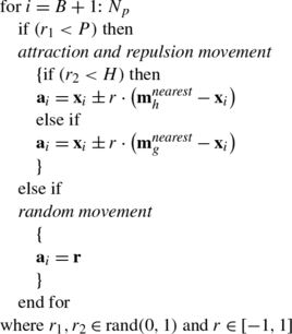
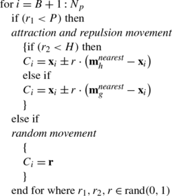
The remaining 6 new positions (a ₅,…,a ₁₀) are individually computed according to step 2 and 3. For such operation, a uniform random number r ₁ is generated within the range [0, 1]. If r ₁ is less than 1−P, the new position a _j (j∈5,…,10) is generated through step 2; otherwise, a _j is obtained from a random re-initialization (step 3) between search bounds.

In order to calculate a new position a _j at step 2, a decision must be made on whether it should be generated by using the elements of M _h or M _g . For such decision, a uniform random number r ₂ is generated within the range [0,1]. If r ₂ is less than H, the new position a _j is generated by using $\mathbf{x}_{j} \pm r \cdot(\mathbf{m}_{h}^{\mathit{nearest}} - \mathbf{x}_{j})$; otherwise, a _j is obtained by considering $\mathbf{x}_{j} \pm r \cdot(\mathbf{m}_{g}^{\mathit{nearest}} - \mathbf{x}_{j})$. Where $\mathbf{m}_{h}^{\mathit{nearest}}$ and $\mathbf{m}_{g}^{\mathit{nearest}}$ represent the closest elements to x _j in memory M _h and M _g respectively. In the first iteration, since there is not available information from previous steps, both memories M _h and M _g share the same information which is only allowed at this initial stage. Figure 2e shows graphically the whole procedure employed by step 2 in order to calculate the new individual position a ₈ whereas Fig. 2f presents the positions of all new individuals (a ₁,a ₂,…,a ₁₀).

Finally, after all new positions (a ₁,a ₂,…,a ₁₀) have been calculated, memories M _h and M _g must be updated. In order to update M _h , new calculated positions (a ₁,a ₂,…,a ₁₀) are arranged according to their fitness values by building vector X=(x ₁,x ₂,…,x ₁₀). Then, the elements of M _h are replaced by the first four elements in X (the best individuals of its generation). In order to calculate the new elements of M _h , current elements of M _h (the present values) and M _g (the updated values) are merged into M _U . Then, by using the dominance concept (explained in Sect. 2.1.5) over M _U , the best four values are selected to replace the elements in M _g . Figure 2g and 2h show the updating procedure for both memories. Applying the dominance (see Fig. 2g), since the distances $a = \mathit{dist}(\mathbf{m}_{h}^{3},\mathbf{m}_{g}^{4}), b = \mathit{dist}(\mathbf{m}_{h}^{2},\mathbf{m}_{g}^{3})$ and $c = \mathit{dist}(\mathbf{m}_{h}^{1},\mathbf{m}_{g}^{1})$ are less than ρ=3, elements with better fitness evaluation will build the new memory M _h . Figure 2h depicts final memory configurations. The circles and solid circles points represent the elements of M _g and M _h respectively whereas the bold squares perform as elements shared by both memories. Therefore, if the complete procedure is repeated over 30 iterations, the memory M _h will contain the 4 global and local maxima as elements. Figure 2i depicts the final configuration after 30 iterations.

3 Circle detection using CAB

In this section, the proposed CAB algorithm is employed for solving the circle detection issue. The detection process is considered similar to a multimodal optimization problem where optimal and suboptimal solutions represent the circular shapes actually present in the image. All global and local minima of J must be found in a single run considering an objective function J:X→ℝ that expresses the coincidence between a candidate solution and an actual circle which is contained in the image. Under such circumstances, a local minimum x _l ∈X of the objective function J:X→ℝ is a solution with J(x _l )≤f(x) for all x neighboring x _l . Under such assumption, if x _l ∈ℝ^N, then ∀x _l ∃ρ>0:J(x _l )≤J(x) ∀x∈X,|x−x _l |≤ρ, where ρ denotes the dominance distance between two solutions. Similarly, a global minimum $\hat{\mathbf{x}}_{g} \in\mathbf{X}$ of the objective function f:X→ℝ is a solution where f(x _g )≤f(x) ∀x∈X.

3.1 Data preprocessing

In order to detect circle shapes, candidate images must be preprocessed first by the well-known Canny algorithm which yields a single-pixel edge-only image. Then, the (x _i ,y _i ) coordinates for each edge pixel p _i are stored inside the edge vector $P = \{ p_{1},p_{2}, \ldots,p_{N_{p}} \}$, with N _p being the total number of edge pixels.

3.2 Individual representation

Each circle C uses three edge points as individuals in the optimization algorithm. In order to construct such individuals, three indexes p _i ,p _j and p _k , are selected from vector P, considering the circle’s contour that connects them. Therefore, the circle C={p _i ,p _j ,p _k } that crosses over such points may be considered as a potential solution for the detection problem. Considering the configuration of the edge points shown by Fig. 3, the circle center (x ₀,y ₀) and the radius r of C can be computed as follows:

(7)

considering

(8)

(9)

and

(10)

being det(.) the determinant and d∈{i,j,k}. Figure 2 illustrates the parameters defined by Eqs. (7) to (10).

Fig. 3

Circle candidate (individual) built from the combination of points p _i , p _j and p _k

3.3 Objective function

In order to calculate the error produced by a candidate solution C, a set of test points is calculated as a virtual shape which, in turn, must be validated, i.e. if it really exists in the edge image. The test set is represented by $S = \{ s_{1},s_{2}, \ldots,s_{N_{s}}\}$, where N _s is the number of points over which the existence of an edge point, corresponding to C, should be validated.

The test point set S is normally generated for most of the approaches [10, 14] by the uniform sampling of the shape boundary. That is, a determined number of test points are generated around the circumference of the candidate circle. Each point s _i is a 2D-point where its coordinates (x _i ,y _i ) are computed using: x _i =x ₀+r⋅cos(2πi/N _s ) and y _i =y ₀+r⋅sin(2πi/N _s ). However, such way of calculating the virtual shape yields several errors. One error case appears when the calculated points S, which correspond to a determined candidate, are compared to an actual dashed circle in the edge image. Under such circumstances, it is possible that any point of S does not find a corresponding edge pixel in the image, although the circle is actually subscribed. Figure 4 displays this issue, with Fig. 4a showing the original pointed image and Fig. 4b representing the set S which has been obtained from the points i, j and k. Figure 4c depicts the comparison between the original circle and the data set S. It is evident that both circles present few coincidences yielding a difficult circle detection task.

Fig. 4

Detection problem due to sampling strategy. (a) shows the original pointed image. (b) represents the set S obtained from the points i, j and k. (c) depicts the comparison between the original circle and the data set S

The most critical error that is produced by the uniform sampling approach is the lack of precision. Such problem is induced by the fact that the number of test points N _s , which are used in the comparison, is fixed. As the number of test points is the same for all circle sizes, the precision in the comparison varies depending on the circle’s size, being less precise as the circles grow larger.

In order to overcome such problems, in our approach, the set S is generated by the Midpoint Circle Algorithm (MCA) [39]. The MCA is a searching method which seeks the required points for drawing a circle digitally. Unlike the uniform sampling approach, MCA calculates the necessary number of test points N _s to totally draw the complete circle, where N _s varies depending of the circle size. In MCA, any point (x,y) on the boundary of the circle with radius r must satisfy the equation f _Circle (x,y)=x ²+y ²−r ². However, MCA avoids computing square-root calculations by comparing the pixel separation distances. The method used for direct distance comparison is to test the halfway position between two pixels (sub-pixel distance) to determine if this midpoint is inside or outside the circle boundary. If the point is in the interior of the circle, the circle function is negative. Thus, if the point is outside the circle, the circle function is positive. Therefore, the error involved in locating pixel positions using the midpoint test is limited to one-half the pixel separation (sub-pixel precision). To summarize, the relative position of any point (x,y) can be determined by checking the sign of the circle function:

(11)

The circle-function test in Eq. (10) is applied to mid-positions between pixels nearby the circle path at each sampling step. Figure 5a shows the midpoint between the two candidate pixels at sampling position x _k .

Fig. 5

(a) Symmetry of a circle: calculation of a circle point (x,y) in one octant yields the circle points shown for other seven octants. (b) Midpoint between candidate pixels at sampling position x _k along a circular path

In MCA the computation time is reduced by considering the symmetry of circles. Circle sections in adjacent octants within one quadrant are symmetric with respect to the 45^∘ line dividing the two octants. These symmetry conditions are illustrated in Fig. 5b, where a point at position (x,y) on a one-eighth circle sector is mapped into the seven circle points in the other octants of the xy plane. Taking advantage of the circle symmetry, it is possible to generate all pixel positions around a circle by calculating only the points within the sector from x=0 to x=y. Thus, in this paper, the MCA is used to calculate the required S points that represent the circle candidate C. The algorithm can be considered as the quickest providing a sub-pixel precision [40]. However, in order to protect the MCA operation, it is important to assure that points lying outside the image plane must not be considered in S.

The objective function J(C) represents the matching error produced between the pixels S of the circle candidate C (food source) and the pixels that actually exist in the edge image, yielding:

(12)

where E(x _i ,y _i ) is a function that verifies the pixel existence in (x _v ,y _v ), with (x _v ,y _v )∈S and N _s being the number of pixels lying on the perimeter corresponding to C currently under testing. Hence, function E(x _v ,y _v ) is defined as:

(13)

A value near to zero of J(C) implies a better response from the “circularity” operator. Figure 6 shows the procedure to evaluate a candidate solution C with its representation as a virtual shape S. In Fig. 6b, the virtual shape is compared to the original image, point by point, in order to find coincidences between virtual and edge points. The virtual shape is built from points p _i , p _j and p _k shown by Fig. 6a. The virtual shape S gathers 56 points (N _s =56) with only 18 of such points existing in both images (shown as blue points plus red points in Fig. 6c) yielding: $\sum_{v = 1}^{N_{s}} E(x_{v},y_{v}) = 18$ and therefore J(C)≈0.67.

Fig. 6

Evaluation of candidate solutions C: the image in (a) shows the original image while (b) presents the virtual shape generated including points p _i , p _j and p _k . The image in (c) shows coincidences between both images marked by blue or red pixels while the virtual shape is also depicted in green (Color figure online)

4 The multiple circle detection procedure

In order to detect multiple circles, most detectors simply apply a one-minimum optimization algorithm, which is able to detect only one circle at a time, repeating the same process several times as previously detected primitives are removed from the image. Such algorithms iterate until there are no more candidates left in the image.

On the other hand, the method used in this paper is able to detect single or multiples circles through only one optimization step. The multi-detection procedure can be summarized as follows: guided by the values of a matching function, the whole group of encoded candidate circles is evolved through the set of evolutionary operators. The best circle candidate (global optimum) is considered to be the first detected circle over the edge-only image. An analysis of the historical memory M _h is thus executed in order to identify other local optima (other circles).

In order to find other possible circles contained in the image, the historical memory M _h is carefully examined. The approach aims to explore all elements, one at a time, assessing which of them represents an actual circle in the image. Since several elements can represent the same circle (i.e. circles slightly shifted or holding small deviations), a distinctiveness factor D _A,B is required to measure the mismatch between two given circles (A and B). Such distinctiveness factor is defined as follows:

(14)

being (x _A ,y _A ) and r _A , the central coordinates and radius of the circle C _A respectively, while (x _B ,y _B ) and r _B represent the corresponding parameters of the circle C _B . One threshold value $E_{s_{TH}}$ is also calculated to decide whether two circles must be considered different or not. Th is computed as:

(15)

where [r _min,r _max] is the feasible radii’s range and d is a sensitivity parameter. By using a high d value, two very similar circles would be considered different while a smaller value for d would consider them as similar shapes. In this work, after several experiments, the d value has been set to 2.

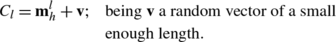
Thus, since the historical memory M _h $\{C_{1}^{\mathbf{M}},C_{2}^{\mathbf{M}}, \ldots,C_{B}^{\mathbf{M}} \}$ groups the elements in descending order according to their fitness values, the first element $C_{1}^{\mathbf{M}}$, whose fitness value represents the best value $J(C_{1}^{\mathbf{M}})$, is assigned to the first circle. Then, the distinctiveness factor $(D_{C_{1}^{\mathbf{M}},C_{2}^{\mathbf{M}}})$ over the next element $C_{2}^{\mathbf{M}}$ is evaluated with respect to the prior $C_{1}^{\mathbf{M}}$. If $D_{C_{1}^{\mathbf{M}},C_{2}^{\mathbf{M}}} > \mathit{Th}$, then $C_{2}^{\mathbf{M}}$ is considered as a new circle otherwise the next element $C_{3}^{\mathbf{M}}$ is selected. This process is repeated until the fitness value $J(C_{i}^{\mathbf{M}})$ reaches a minimum threshold J _TH . According to such threshold, other values above J _TH represent individuals (circles) that are considered as significant while other values lying below such boundary are considered as false circles and hence they are not contained in the image. After several experiments the value of J _TH is set to $(J(C_{1}^{\mathbf{M}})/10)$.

The fitness value of each detected circle is characterized by its geometric properties. Big and well-drawn circles normally represent points in the search space with higher fitness values whereas small and dashed circles describe points with lower fitness values. Likewise, circles with similar geometric properties, such as radius, size, etc., tend to represent locations holding similar fitness values. Considering that the historical memory M _h groups the elements in descending order according to their fitness values, the proposed procedure allows the cancelling of those circles which belong to the same circle and hold a similar fitness value.

4.1 Implementation of CAB strategy for circle detection

The implementation of the proposed algorithm can be summarized in the following steps:

• Step 1: Adjust the algorithm parameters N _p , B, H, P, NI and d.

• Step 2: Randomly generate a set of N _p candidate circles (position of each animal) $\mathbf{C} = \{ C_{1},C_{2}, \ldots,C_{N_{p}}\}$ set using Eq. (1).

• Step 3: Sort C according to the objective function (dominance) to build $\mathbf{X} = \{ \mathbf{x}_{1},\mathbf{x}_{2}, \ldots,\mathbf{x}_{N_{p}}\}$.

• Step 4: Choose the first B positions of X and store them into the memory M _g .

• Step 5: Update M _h according to Sect. 2.1.5. (during the first iteration: M _h =M _g ).

• Step 6: Generate the first B positions of the new solution set C ({C ₁,C ₂,…,C _B }). Such positions correspond to the elements of M _h making a slight random perturbation around them.

  

• Step 7: Generate the rest of the C elements using the attraction, repulsion and random movements.

  

• Step 8: If NI is not completed, the process go back to step 3. Otherwise, the best values in $\mathbf{M}_{h} \{ C_{1}^{\mathbf{M}},C_{2}^{\mathbf{M}}, \ldots,C_{B}^{\mathbf{M}} \}$ represents the best solutions (the best found circles).

• Step 9: The element with the highest fitness value $J(C_{1}^{\mathbf{M}})$ is identified as the first circle C ₁.

• Step 10: The distinctiveness factor $D_{C_{m}^{\mathbf{M}},C_{m - 1}^{\mathbf{M}}}$ of circle $C_{m}^{\mathbf{M}}$ (element m) with the next highest probability is evaluated with respect to $C_{m - 1}^{\mathbf{M}}$. If $D_{C_{m}^{\mathbf{M}},C_{m - 1}^{\mathbf{M}}} > \mathit{Th}$, then it is considered $C_{m}^{\mathbf{M}}$ as a new circle otherwise the next action is evaluated.

• Step 11: The step 10 is repeated until the element’s fitness value reaches $(J(C_{1}^{\mathbf{M}})/10)$.

The number of candidate circles N _p is set considering a balance between the number of local minima to be detected and the computational complexity. In general terms, a large value of N _p suggests the detection of a great amount of circles at the cost of excessive computer time. After exhaustive experimentation, it has been found that a value of N _p =30 represents the best trade-off between computational overhead and accuracy and therefore such value is used throughout the study.

5 Experimental results

Experimental tests have been developed in order to evaluate the performance of the circle detector. The experiments address the following tasks:

• (1) Circle localization,

• (2) Shape discrimination,

• (3) Circular approximation: occluded circles and arc detection.

Table 1 presents the parameters for the CAB algorithm at this work. They have been kept for all test images after being experimentally defined.

Table 1 CAB detector parameters

5.1 Circle localization

5.1.1 Synthetic images

The experimental setup includes the use of several synthetic images of 400×300 pixels. All images contain a different amount of circular shapes and some have also been contaminated by added noise as to increase the complexity of the localization task. The algorithm is executed over 50 times (in order to assure consistency) for each test image, successfully identifying and marking all required circles in the image. The detection has proved to be robust to translation and scaling still offering a reasonably low execution time. Figure 7 shows the outcome after applying the algorithm to two images from the experimental set.

Fig. 7

Circle localization over synthetic images. The image (a) shows the original image while (b) presents the detected circles as an overlay. The image in (c) shows a second image with salt & pepper noise and (d) shows detected circles as a red overlay (Color figure online)

5.1.2 Natural images

This experiment tests the circle detection on several real images of 640×480 pixels. All images contain a different number of circular shapes; images were captured with a digital camera in an 8-bit format. Each image is pre-processed by the algorithm of Canny edge detection, after having been processed image is introduced to the CAB algorithm for the detection of circles. Figure 8 shows the results after applying the algorithm CAB.

Fig. 8

Circle detection algorithm over natural images: the image in (a) shows the original image while (b) presents the detected circles as a red overlay (Color figure online)

5.2 Shape discrimination tests

In this section we will observe the ability of the algorithm to detect circular patterns through different forms present in the image. Figure 9 shows four shapes in the image of 500×300 pixels with added noise makes the detection of circles. Figure 10 repeats the experiment over real-life images.

Fig. 9

Shape discrimination over synthetic images: (a) shows the original image contaminated by salt & pepper noise while (b) presents the detected circle as an overlay

Fig. 10

Shape discrimination in real-life images: (a) shows the original image and (b) presents the detected circle as an overlay

5.3 Circular approximation: occluded circles and arc detection

The CAB detector algorithm is able to detect occluded or imperfect circles as well as partially defined shapes such as arc segments. The relevance of such functionality comes from the fact that imperfect circles are commonly found in typical computer vision applications. Since circle detection has been considered as an optimization problem, the CAB algorithm allows finding circles that may approach a given shape according to fitness values for each candidate. Figure 11a shows some examples of circular approximation. Likewise, the proposed algorithm is able to find circle parameters that better approach an arc or an occluded circle. Figure 11b and 11c show some examples of this functionality. A small value for J(C), i.e., near zero, refers to a circle while a slightly bigger value accounts for an arc or an occluded circular shape. Such a fact does not represent any trouble as circles can be shown following the obtained J(C) values.

Fig. 11

CAB Approximating circular shapes and arc detections

5.4 Performance comparison

In order to analyse the performance of the proposed approach, it is compared to other circle detectors presented in the literature. The experiments are organized by considering two different comparisons: comparisons to other evolutionary methods and one comparison to a Hough transform-based detector. In each set of experiments a different set of test images has been chosen in order to enhance the overall analysis.

5.5 Comparison to other evolutionary methods

In these experiments, it is analyzed the performance of the proposed algorithm against other similar evolutionary approaches such as the GA-based algorithm [10] and the BFAO detector [14].

The GA-based algorithm follows the proposal of Ayala-Ramirez et al. [10], which considers the population size as 70, the crossover probability as 0.55, the mutation probability as 0.10 and the number of elite individuals as 2. The roulette wheel selection and the 1-point crossover operator are both applied. The parameter setup and the fitness function follow the configuration suggested in [10]. The BFAO algorithm follows the implementation from [14] considering the experimental parameters as: S=50, N _c =350, N _s =4, N _ed=1, P _ed=0.25, d _attract=0.1, w _attract=0.2, w _repellant=10h _repellant=0.1, λ=400 and ψ=6. Such values are found to be the best configuration set according to [14]. Both, the GA-based algorithm and the BAFO method use the same objective function that is defined by Eq. (12).

Images rarely contain perfectly-shaped circles. Therefore, with the purpose of testing accuracy for a single-circle, the detection is challenged by a ground-truth circle which is determined from the original edge map. The parameters (x _true ,y _true ,r _true ) representing the testing circle are computed using the Eqs. (6)–(9) for three circumference points over the manually-drawn circle. Considering the centre and the radius of the detected circle are defined as (x _D ,y _D ) and r _D , the Error Score (Es) can be accordingly calculated as:

(16)

The central point difference (|x _true −x _D |+|y _true −y _D |) represents the centre shift for the detected circle as it is compared to a benchmark circle. The radio mismatch (|r _true −r _D |) accounts for the difference between their radii. η and μ two weighting parameters which are to be applied separately to the central point difference and to the radio mismatch for the final error Es. At this time, they are chosen as η=0.05 and μ=0.1. Such particular choice ensures that the radii difference would be strongly weighted in comparison to the difference of central circular positions between the manually detected and the machine-detected circles. Here we assume that if Es is found to be less than 1, then the algorithm gets a success, otherwise, we say that it has failed to detect the edge-circle. Note that for η=0.05 and μ=0.1; Es<1 means the maximum difference of radius tolerated is 10 while the maximum mismatch in the location of the center can be 20 (in number of pixels). In order to appropriately compare the detection results, the Detection Rate (DR) is introduced as a performance index. DR is defined as the percentage of reaching detection success after a certain number of trials. For “success” it does mean that the compared algorithm is able to detect all circles contained in the image, under the restriction that each circle must hold the condition Es<1. Therefore, if at least one circle does not fulfil the condition of Es<1, the complete detection procedure is considered a failure.

In order to use an error metric for multiple-circle detection, the averaged Es produced from each circle in the image is considered. Such criterion, defined as the Multiple Error (ME), is calculated as follows:

(17)

where NC represents the number of circles within the image according to a human expert.

Figure 12 shows three synthetic images and the resulting images after applying the GA-based algorithm [8], the BFOA method [12] and the proposed approach. Figure 13 presents experimental results considering three natural images. The performance is analyzed by considering 35 different executions for each algorithm. Table 2 shows the averaged execution time, the detection rate in percentage and the averaged multiple error (ME), considering six test images (shown by Figs. 12 and 13). The best entries are bold-cased in Table 2. Close inspection reveals that the proposed method is able to achieve the highest success rate keeping the smallest error, still requiring less computational time for the most cases.

Fig. 12

Synthetic images and their detected circles for: GA-based algorithm, the BFOA method and the proposed CAB algorithm

Fig. 13

Real-life images and their detected circles for: GA-based algorithm, the BFOA method and the proposed CAB algorithm

Table 2 The averaged execution-time, detection rate and the averaged multiple error for the GA-based algorithm, the BFOA method and the proposed CAB algorithm, considering six test images (shown by Figs. 8 and 9)

In order to statistically analyze the results in Table 2, a non-parametric significance proof known as the Wilcoxon’s rank test [41–43] for 35 independent samples has been conducted. Such proof allows assessing result differences among two related methods. The analysis is performed considering a 5 % significance level over multiple error (ME) data. Table 3 reports the p-values produced by Wilcoxon’s test for a pair-wise comparison of the multiple error (ME), considering two groups gathered as CAB vs. GA and CAB vs. BFOA. As a null hypothesis, it is assumed that there is no difference between the values of the two algorithms. The alternative hypothesis considers an existent difference between the values of both approaches. All p-values reported in the Table 3 are less than 0.05 (5 % significance level) which is a strong evidence against the null hypothesis, indicating that the best CAB mean values for the performance are statistically significant which has not occurred by chance.

Table 3 p-values produced by Wilcoxon’s test comparing CAB to GA and BFOA over the averaged ME from Table 2

5.6 Comparison to Hough transform-based detectors

Images are often deteriorated by noise due to various sources of interference and other phenomena that affect the measurement in imaging and data acquisition systems. Classical methods face great difficulties in detecting parametric shapes within images containing noise and distortions [8]. In this section, our approach is compared to other Hough transform-based detectors such as the RHT in terms of robustness and efficiency. The RHT algorithm in the experiments has been implemented following the configuration described in [4].

Figure 14 shows the relative performance of CAB in comparison to the RHT algorithm. All images contain different noise conditions in order to hinder the detection task. The performance analysis is achieved by considering 35 different executions for each algorithm over the three images. The results, exhibited in Fig. 14, present the median-run solution (when the runs were ranked according to their final ME value) obtained throughout the 35 runs. Table 4 reports the corresponding averaged execution time, detection rate (in %), and average multiple error (using (10)) for CAB and RHT algorithms over the set of images (the best results are bold-cased). According to such results, the RHT algorithm presents a success rate of 100 % when the images are noise-free. However, just as the noise increases, the success rate drastically decreases to 11 %. Different to RHT, the CAB algorithm maintains the same detection performance for all experiments. Such behavior indicates that the RHT method is failure-prone depending on the noise level whereas the CAB algorithm is more robust for detecting circles despite noisy conditions. On the other hand, the CAB algorithm presents a better efficiency, since it shows the best performance indexes in terms of the elapsed time (average time) and the precision (multiple error).

Fig. 14

Relative performance of the CAB compared with the RHT

Table 4 Average time, detection rate and averaged error for CAB and HT, considering three test images

6 Conclusions

This paper has presented an algorithm for the automatic detection of multiple circular shapes from complicated and noisy images without considering the conventional Hough transform principles. The detection process is considered to be similar to a multi-modal optimization problem. In contrast to other heuristic methods that employ an iterative procedure, the proposed CAB method is able to detect single or multiple circles over a digital image by running only one optimization cycle. The CAB algorithm searches the entire edge-map for circular shapes by using a combination of three non-collinear edge points as candidate circles (animal positions) in the edge-only image. A matching function (objective function) is used to measure the existence of a candidate circle over the edge-map. Guided by the values of such matching function, the set of encoded candidate circles is evolved using the CAB algorithm so that the best candidate can be fitted into an actual circle. After the optimization has been completed, an analysis of the embedded memory is executed in order to find the significant local minima (remaining circles). The overall approach generates a fast sub-pixel detector which can effectively identify multiple circles in real images despite some circular objects exhibit a significant occluded portion.

Classical Hough transform methods for circle detection use three edge points to cast a vote for the potential circular shape in the parameter space. However, they would require a huge amount of memory and longer computational times to obtain a sub-pixel resolution. Moreover, HT-based methods rarely find a precise parameter set for a circle in the image [44]. In our approach, the detected circles hold a sub-pixel accuracy inherited directly from the circle equation and the MCA method.

In order to test the circle detection performance, both speed and accuracy have been compared. Score functions are defined by Eqs. (15) and (16) in order to measure accuracy and effectively evaluate the mismatch between manually detected and machine-detected circles. We have demonstrated that the CAB method outperforms both the GA (as described in [8]) and the BFOA (as described in [12]) within a statistically significant framework (Wilcoxon test). In contrast to the CAB method, the RHT algorithm [4] shows a decrease in performance under noisy conditions. Yet the CAB algorithm holds its performance under the same circumstances. Finally, Table 2 indicates that the CAB method can yield better results on complicated and noisy images compared with the GA and the BFOA methods. However, the aim of this study is not to beat all circle detection methods proposed earlier, but to show that the CAB algorithm can effectively serve as an attractive method to successfully extract multiple circular shapes.

References

da Fontoura Costa L, Marcondes Cesar R, Jr (2001) Shape analysis and classification. CRC Press, Boca Raton
Atherton TJ, Kerbyson DJ (1993) Using phase to represent radius in the coherent circle hough transform. In: Proc, IEE colloquium on the hough transform. IEE, London
Shaked D, Yaron O, Kiryati N (1996) Deriving stopping rules for the probabilistic Hough transform by sequential analysis. Comput Vis Image Underst 63:512–526
Xu L, Oja E, Kultanen P (1990) A new curve detection method: randomized Hough transform (RHT). Pattern Recognit Lett 11(5):331–338
Han JH, Koczy LT, Poston T (1993) Fuzzy Hough transform. In: Proc 2nd int conf on fuzzy systems, vol 2, pp 803–808
Becker J, Grousson S, Coltuc D (2002) From Hough transforms to integral geometry. In: Proc int geoscience and remote sensing symp, 2002 IGARSS_02, vol 3, pp 1444–1446
Jiang L (2012) Efficient randomized Hough transform for circle detection using novel probability sampling and feature points. Optik 123(10):1834–1840
Valova I, Milano G, Bowen K, Gueorguieva N (2011) Bridging the fuzzy, neural and evolutionary paradigms for automatic target recognition. Appl Intell 35(2):211–225
An S-Y, Kang J-G, Choi W-S, Oh S-Y (2011) A neural network based retrainable framework for robust object recognition with application to mobile robotics. Appl Intell 35(2):190–210
Ayala-Ramirez V, Garcia-Capulin CH, Perez-Garcia A, Sanchez-Yanez RE (2006) Circle detection on images using genetic algorithms. Pattern Recognit Lett 27:652–657
Cuevas E, Ortega-Sánchez N, Zaldivar D, Pérez-Cisneros M (2012) Circle detection by harmony search optimization. J Intell Robot Syst 66(3):359–376
Cuevas E, Oliva D, Zaldivar D, Pérez-Cisneros M, Sossa H (2012) Circle detection using electro-magnetism optimization. Inf Sci 182(1):40–55
Cuevas E, Zaldivar D, Pérez-Cisneros M, Ramírez-Ortegón M (2011) Circle detection using discrete differential evolution optimization. PAA Pattern Anal Appl 14(1):93–107
Dasgupta S, Das S, Biswas A, Abraham A (2010) Automatic circle detection on digital images with an adaptive bacterial foraging algorithm. Soft Comput 14(11):1151–1164
Li Y, Zeng X (2010) Multi-population co-genetic algorithm with double chain-like agents structure for parallel global numerical optimization. Appl Intell 32(3):292–310
Das S, Maity S, Qub B, Suganthan PN (2011) Real-parameter evolutionary multimodal optimization—a survey of the state-of-the-art. Swarm Evol Comput 1:71–88
Goldberg DE, Richardson J (1987) Genetic algorithms with sharing for multimodal function optimization. In: Proc of the second international conference on genetic algorithms (ICGA), New Jersey
Kennedy J, Eberhart RC (1995) Particle swarm optimization. In: Proceedings of the 1995 IEEE international conference on neural networks, vol 4, pp 1942–1948
Norouzzadeh MS, Ahmadzadeh MR, Palhang M (2012) LADPSO: using fuzzy logic to conduct PSO algorithm. Appl Intell 37(2):290–304
Ben Ali YM (2012) Psychological model of particle swarm optimization based multiple emotions. Appl Intell 36(3):649–663
Liang J, Qin AK, Suganthan PN (2006) Comprehensive learning particle swarm optimizer for global optimization of multi-modal functions. IEEE Trans Evol Comput 10(3):281–295
Chen DB, Zhao CX (2009) Particle swarm optimization with adaptive population size and its application. Appl Soft Comput 9(1):39–48
Xu Q, Lei W, Si J (2010) Predication based immune network for multimodal function optimization. Eng Appl Artif Intell 23:495–504
Sumper D (2006) The principles of collective animal behaviour. Philos Trans R Soc Lond B, Biol Sci 361(1465):5–22
Petit O, Bon R (2010) Decision-making processes: the case of collective movements. Behav Process 84:635–647
Kolpas A, Moehlis J, Frewen T, Kevrekidis I (2008) Coarse analysis of collective motion with different communication mechanisms. Math Biosci 214:49–57
Couzin I (2008) Collective cognition in animal groups. Trends Cogn Sci 13(1):36–43
Couzin ID, Krause J (2003) Self-organization and collective behavior in vertebrates. Adv Study Behav 32:1–75
Bode N, Franks D, Wood A (2010) Making noise: emergent stochasticity in collective motion. J Theor Biol 267:292–299
Couzi I, Krause I, James R, Ruxton G, Franks N (2002) Collective memory and spatial sorting in animal groups. J Theor Biol 218:1–11
Couzin ID (2007) Collective minds. Nature 445:715–728
Bazazi S, Buhl J, Hale JJ, Anstey ML, Sword GA, Simpson SJ, Couzin ID (2008) Collective motion and cannibalism in locust migratory bands. Curr Biol 18:735–739
Hsu Y, Earley R, Wolf L (2006) Modulation of aggressive behaviour by fighting experience: mechanisms and contest outcomes. Biol Rev 81(1):33–74
Ballerini M (2008) Interaction ruling collective animal behavior depends on topological rather than metric distance: evidence from a field study. Proc Natl Acad Sci USA 105:1232–1237
Yang X-S (2008) Nature-inspired metaheuristic algorithms. Luniver Press, Beckington
Gandomi AH, Yang X-S, Alavi AH (2011) Cuckoo search algorithm: a metaheuristic approach to solve structural optimization problems. Eng Comput. doi:10.1007/s00366-011-0241-y
Zang H, Zhang S, Hapeshi K (2010) A review of nature-inspired algorithms. J Bionics Eng 7:S232–S237
Gandomi A, Alavi A (2012) Krill herd: a new bio-inspired optimization algorithm. Commun Nonlinear Sci Numer Simul 17:4831–4845
Bresenham JE (1977) A linear algorithm for incremental digital display of circular arcs. Commun ACM 20:100–106
Van Aken JR (2005) Efficient ellipse-drawing algorithm. IEEE Comput Graph Appl 4(9):24–35
Wilcoxon F (1945) Individual comparisons by ranking methods. Biometrics 1:80–83
Garcia S, Molina D, Lozano M, Herrera F (2008) A study on the use of non-parametric tests for analyzing the evolutionary algorithms’ behaviour: a case study on the CEC’2005 special session on real parameter optimization. J Heuristics. doi:10.1007/s10732-008-9080-4
Santamaría J, Cordón O, Damas S, García-Torres JM, Quirin A (2008) Performance evaluation of memetic approaches in 3D reconstruction of forensic objects. Soft Comput. doi:10.1007/s00500-008-0351-7
Chen T-C, Chung K-L (2001) An efficient randomized algorithm for detecting circles. Comput Vis Image Underst 83:172–191
Author information
Authors and Affiliations
Corresponding author
Rights and permissions
About this article
Cite this article
Cuevas, E., González, M. Multi-circle detection on images inspired by collective animal behavior. Appl Intell 39, 101–120 (2013). https://doi.org/10.1007/s10489-012-0396-2
Published:
Issue Date:
DOI: https://doi.org/10.1007/s10489-012-0396-2