Flexible dynamic sustainable procurement model

Abstract

Management of global supply chains is a challenging task due to the uncertainties leading to supply chain disruption. This requires the supply chains to be not only effective and efficient but also flexible in their operations to mitigate these disruptions. It has been observed that supply chains are mostly influenced by suppliers and carriers; hence, a business firm needs to be flexible and sustainable in selection of suppliers and carriers to overcome any disruptions. This paper proposes a flexible dynamic sustainable procurement (FDSP) framework for global supply chains by considering not only qualitative parameters such as quality, reliability, social and environmental factors for the selection of suppliers as well as carriers but also taking into account quantitative preferences such as cost, supplier capacity and carrier capacity. However, independently using quantitative parameters might allocate order quantities to the suppliers and carriers which are least preferred based on other qualitative parameters. Therefore, the proposed FDSP model provides flexibility by integrating the quantitative and qualitative parameters to allocate order quantities to suppliers and carriers preferred by both the sets. Hence, the proposed FDSP model provides a range of possible integrated solutions and business firm can select the best suited solution having least deviation. The deviations are computed from integrated optimal solution provided by FDSP and quantitative models. The proposed FDSP model is solved for a case illustration to demonstrate the proposed framework.

1 Introduction

Procurement optimization in global supply chains is the most challenging and emerging activity drawing the attention of researchers and practitioners towards the complexity of the problem. The evolution of procurement from purchasing which was considered merely a clerical function to a more complex strategic decision has called for an increased research in this area. Procurement involves wide range of activities ranging from identification of sources and allocation of required part quantities to the transportation options available for procurement. It has been realized that procurement costs contributes to about 60% of the cost of finished product (De Boer et al. 2001), making procurement even more important for a firm’s business performance in terms of revenue generation or cost minimization. The firm relies on various suppliers located in geographically distant regions. Suppliers in turn also relies on various carriers for supplying products to buying firm, therefore, selection of carriers is also an integral part of procurement function (Songhori et al. 2011; Choudhary and Shankar 2013). Procurement deals with several supply chain linkages and, hence, an effective management of all the linkages is required in order to avoid any supply chain disruptions.

Moreover, recent emphasis on sustainable business practices has led business firms to estimate and manage carbon emissions in the entire procurement process. Ample amount of research work is done to rank the suppliers based on several qualitative parameters such as reliability, quality, service level, sustainability, etc. to ensure the selection of most suitable suppliers. Similarly, research has also been done on selection of carriers using qualitative parameters. There are numerous models in literature for lot-sizing, supplier selection and carrier selection addressed individually. However, there is very little research done on integration of supplier selection and carrier selection in integrated procurement decisions. Mostly, the research in procurement is clearly divided into qualitative and quantitative approaches used independently, but integration of these approaches is not very well attempted. Therefore, this paper proposes an integrated approach for flexible dynamic sustainable procurement (FDSP) by integrating qualitative models for selection of suppliers as well as carriers and quantitative model for procurement to optimize total procurement cost. The proposed FDSP model provides a range of possible integrated solutions and business firm can select the best suited solution having least deviation. The deviations are computed from integrated optimal solution provided by FDSP and quantitative models. The proposed FDSP model is solved for a case illustration to demonstrate the proposed framework.

The rest of the paper is organized as follows. Section 2 provides a detailed literature review about procurement problem. Section 3 discusses the entire framework for flexible dynamic sustainable procurement (FDSP) followed by modelling of the flexible dynamic sustainable procurement in Sect. 4. Section 5 demonstrates the FDSP with the help of a case illustration and provides discussion on results obtained. Section 6 presents managerial insights, contributions and limitations followed by conclusion and future scope of work.

2 Literature review

This section studies different qualitative and quantitative techniques used in literature to address procurement problem.

2.1 Qualitative models in procurement

In procurement problem, the firm is dealing with multiple suppliers and logistics providers in order to obtain raw materials for fulfilling demand in time. There are many qualitative parameters such as reliability, market reputation and financial stability which any buying firm keeps in mind before allocating orders to respective suppliers and carriers. Therefore, the qualitative modelling for selection of suppliers as well as carriers is essential for formulation of a dynamic procurement problem. There is a plethora of work in literature on development of models for identification and selection of suppliers for procurement based on a various criteria. Various MCDM techniques are used independently or in integration with other techniques for selection of suppliers. Ghodsypour and O’Brien (1998), Handfield et al. (2002), Wang et al. (2004) and Xia and Wu (2007) have applied AHP for qualitative modelling. Other MCDM techniques such as TOPSIS (Shyur and Shih 2006), IRP (Ware et al. 2014a), W-IRP (Kumar and Singh 2015; Kaur et al. 2016) are also widely used in literature to model qualitative factors for supplier selection in a procurement problem. However, sometimes it is difficult to comprehend the vagueness in expert opinions and hence, fuzzy numbers are used to address the problem. Chan et al. (2008), Kahraman et al. (2003) and Haq and Kannan (2006) have used Fuzzy AHP whereas Chen et al. (2006) have used fuzzy TOPSIS for qualitative modelling of procurement problem.

Logistics is also an important procurement function and there are many qualitative factors such as schedule delivery reliability and lead times are considered during selection of logistics services in procurement. This has drawn the attention of researchers and practitioners towards this problem. In literature, there are few attempts for qualitative modelling of the carrier selection problem. Fraering and Prasad (1999) developed initial qualitative model for global sourcing and logistics decision by considering total cost of ownership. Stank and Goldsby (2000) proposed a qualitative framework for transportation decisions in procurement problem. Vijayvargiya and Dey (2010) used AHP approach for carrier selection based on traditional criteria such as cost, delivery and value added services. Lin and Yeh (2013) considered multi-commodity reliability as an important performance criterion for qualitative modelling of carrier selection problem. Similarly, Yang and Regan (2013) proposed MCDM based methodology for logistics in procurement. However, the models discussed above do not consider sustainability as a criteria for carrier selection.

Both supplier selection and carrier selection are modelled as MCDM problem in literature, widely using one technique or integrating two techniques together. But the integration of various MCDM techniques into a single model is not very well attempted in literature. It is also observed that much work has done in qualitative modelling of suppliers and carriers independently; however, the joint qualitative modelling of suppliers and carriers is not addressed so far.

2.2 Quantitative models in procurement

There is a plethora of work in literature on development lot-sizing models for procurement. Initially the problem was studied as a dynamic lot-sizing problem, focussing order allocations to optimize holding and ordering costs only (Wagner and Whitin 1958). But later it was realized that as procurement is a multi sourcing problem (Aissaoui et al. 2007), it is essential to incorporate supplier selection in lot-sizing models to address procurement. The first model integrating supplier selection and lot-sizing was proposed for the case of Australian post (Gaballa 1974). Ghodsypour and O’Brien (2001) modified Economic Ordering Quantity (EOQ) model to integrate supplier selection and lotsizing in procurement. In this direction Tsiakis et al. (2001), Swenseth and Godfrey (2002), Kelle et al. (2003), Chiang and Russell (2004), Purohit et al. (2016a), Li et al. (2015) have incorporated lot-sizing and supplier selection into procurement model. Ware et al. (2014b) have emphasized the importance of supplier selection into procurement decisions by considering penalties to handle late deliveries. Li (2015) proposed supplier selection and lot-sizing problem by incorporating risk.

Recently, the procurement decisions are also being influenced by world-wide carbon regulatory legislations, resulting in incorporation of carbon calculation and management in procurement models. Benjaafar et al. (2013) proposed lot-sizing models for various scenarios incorporating carbon emissions as a core issue. The sustainable models are also proposed by Hsu et al. (2011), Ubeda et al. (2011), Jaber et al. (2013), Purohit et al. (2016b), for lot-sizing problem only. The carbon emissions associated with supplier and carrier selection are not considered. The emphasis on carbon emissions and huge transportation costs has also encouraged researchers to incorporate logistics in procurement models. The research work by Cholette and Venkat (2009) and Ubeda et al. (2011) have incorporated carbon emissions from logistics into their models. Similarly, Bonney and Jaber (2011) considered vehicle emissions in EOQ model to determine lot-sizes in procurement. However, the model is restricted due to the limitations of EOQ. Recently, Basu et al. (2016) modelled emissions caused by logistics in procurement. However, the problem is route optimization and a single supplier is considered only.

Table 1 Summary of reviewed literature

Some of the research work by Liao and Rittscher (2007), Songhori et al. (2011) and Kaur and Singh (2016) have proposed integrated procurement models by jointly addressing lot-sizing, supplier selection and carrier selection under various business scenarios. However, the models address only quantitative aspects and do not consider qualitative criteria in selection of suppliers and carriers. Summary of reviewed literature is provided in Table 1. It can be seen from the table that extensive work has been also done in the past to select suppliers and carriers using these quantified qualitative factors. In the past, extensive research work has been also carried out in the procurement problem through quantitative modelling such as MINLP/MILP. In some cases, these quantitative models do also select suppliers and carriers in some way.

So far the research work available on supplier and/or carrier selection either through qualitative modelling or quantitative modelling does not provide comparable results. For example, the suppliers or carriers which are poorly ranked through the qualitative modelling are being selected in the qualitative modelling owing to low cost parameters or high capacities (supplier/carrier). This creates a big contradiction between the supplier/carrier selection using qualitative and quantitative approaches. However, the supplier/ carrier selection results should be similar. The difference in supplier/carrier selection using quantitative and qualitative models is due to missing links between these two. Therefore, the proposed FDSP framework links qualitative modelling and quantitative modelling together and integrates the qualitative modelling of supplier/carrier selection by providing its outcome as an input into the quantitative modelling of dynamic procurement problem. This further reassigns the order allocation and supplier/carrier selection by considering qualitative and quantitative models together.

Due to this, the proposed FDSP framework provides a range of solution towards optimization of procurement cost by minimum possible order allocation to the poorly ranked suppliers and/or carriers. The major contribution of the proposed FDSP model is to provide a range of such possible solutions and provides various possible options to the organization using the deviational matrix to select the best suited options. The proposed FDSP framework is different from the previous models (Songhori et al. 2011; Choudhary and Shankar 2013; Kaur and Singh 2016), where either the supplier/carrier selections are made or procurement problem is modelled considering sets of suppliers/carriers. These available models do not integrate the outcome of qualitative models into quantitative models or other way round. The proposed FDSP model develops elimination strategies based on the outcomes from qualitative modelling of suppliers/carriers. Therefore, this paper is an attempt to address both qualitative models and quantitative models in one framework and providing the required flexibility and minimizing the allocations to least preferred suppliers and carriers. The working methodology of the proposed FDSP framework is discussed in Sect. 3.

3 Flexible dynamic sustainable procurement (FDSP) framework

In this section, Flexible Dynamic Sustainable Procurement (FDSP) framework is explained. The proposed framework integrates the qualitative models for the identification and selection of the most and the least preferred suppliers and carriers, and the quantitative model for optimal order allocation, supplier and carrier selection. The framework is both ‘flexible’ and ‘dynamic’ at the same time. In this framework, the term flexible is referred to the various options a firm can use to select the is having the best procurement plan considering various factors such as elimination of poorly ranked suppliers as well as carriers. On the other hand the term dynamic is referred to the presence of lot sizing over multiple periods. The dynamic term is used with reference to the index of time that has been taken to make the procurement problem a dynamic one.

In the proposed FDSP framework, the quantitative approaches provide an optimal solution based on quantitative parameters such as cost, lead time, supplier capacity and carrier capacity. However, the quantitative model ignores the firm’s preferences for suppliers or carriers based on many qualitative parameters. It is seen that in real practice, the firm’s preferences for suppliers and carriers based on several qualitative parameters such as reliability, quality, service level and sustainability while allocation of orders is extremely important. But the quantitative models are generally based on cost minimization and allocate orders to suppliers and carriers based on parameters such as lead-time, supplier capacity and carrier capacity and cost. Using purely quantitative model might allocate orders to least preferred suppliers and carriers. To overcome this issue, FDSP framework is proposed which incorporates the flexibility to eliminate poorly ranked suppliers and carriers by minimizing the deviation from objective function of dynamic sustainable procurement problem. The proposed FDSP framework is shown in Fig. 1.

Fig. 1

Flexible dynamic sustainable procurement (FDSP) framework

4 Flexible dynamic sustainable procurement (FDSP) model

The section models the proposed FDSP. To model FDSP, qualitative model is provided in Sect. 4.1 to take care of carrier and supplier selection while quantitative model is developed in Sect. 4.2 to minimize procurement cost in a carbon trading environment for DSP. Finally, Sect. 4.3 presents an integrated approach of qualitative and quantitative models to develop FDSP.

4.1 Phase I: qualitative models

Qualitative models are mostly used to rank suppliers and carriers for given set of qualitative criteria. However, the set of criteria and weightages given to each criterion may vary across industries, regions and sectors. Following are the qualitative models used to rank suppliers and carriers.

Analytical hierarchy process (AHP): AHP is proposed by Saaty (1980) is most widely used to solve multi criteria decision making problems. The technique involves ranking the set of alternatives for given criteria.

Technique for order preference by similarity to ideal solution (TOPSIS): TOPSIS (proposed by Hwang and Yoon 1981) is a compromise method in which the alternative closest to ideal solution (which maximizes advantages criteria) and farthest from negative ideal solution (which minimizes advantages criteria) is chosen.

Interpretive ranking process (IRP):: Proposed by Sushil (2009) and is used to develop interpretive models between criteria and alternatives.

Weighted interpretive ranking process (W-IRP): Recently proposed by Kumar and Singh (2015), considers the weightages of each criteria in IRP, where IRP considers equal weights for all criteria.

Borda–Kendall (BAK) technique: It aggregates ranks from various qualitative models for each supplier and/carrier and is widely used because of its computational simplicity (Cook and Seiford 1982; Jensen 1986).

Integer linear program (ILP): Proposed by Kaur et al. (2016) to provide integrated rank of alternatives from the sets of ranks provided by other qualitative models. ILP minimize the total deviation of the integrated rank from all ranks obtained from different qualitative models. The ILP formulation for aggregated/integrated rank based on inputs from other MCDM techniques is shown below. Let $R_{pq}$ is the rank of pth supplier/carrier using qth MCDM technique while $R'_{p}$ is the aggregated/integrated final rank of the pth suppliers/carriers. Also, P is the total number of suppliers/carriers and Q is the number of MCDM techniques.

Objective function

$$\begin{aligned} Min\,Z=\sum \limits _{p=1}^P \sum \limits _{q=1}^Q \left| {R_{pq} -R^{\prime }_p} \right| \end{aligned}$$

(I)

Subject to

$$\begin{aligned} 1\le R^{\prime }_p \le p\qquad \forall p\left( {1,2,\ldots ,P} \right) \end{aligned}$$

(II)

$$\begin{aligned} R^{\prime }_{p}\ne R^{\prime }_{p+1} \qquad \forall p\left( {1,2,\ldots ,P} \right) \end{aligned}$$

(III)

$$\begin{aligned} R^{\prime }_p~is~an~integer \qquad \forall p \left( {1,2,\ldots ,P} \right) \end{aligned}$$

(IV)

The objective function of the ILP is to minimize the total difference between the ranks obtained by suppliers/carriers using various MCDM techniques and the final aggregated rank as shown in equation (I). Equation (II) bounds the aggregated rank values to the maximum number of attributes (suppliers/carriers). Equation (III) suggests that no two aggregate ranks can take same value. Equation (IV) restricts the aggregated rank values to be integer values only.

4.1.1 Qualitative model for supplier selection

In supplier selection, a set of criteria is identified which are used to evaluate the suppliers. MCDM techniques such as AHP, TOPSIS, IRP, W-IRP and BAK can be applied. Expert opinion is used to generate pair-wise comparison matrices involved in these techniques Supplier rankings derived from various MCDM techniques may or may not be the same. ILP is used to obtain final supplier ranking having minimum total deviations among the supplier rankings given by all MCDM techniques. Applying proposed qualitative model, the set of most and least preferred suppliers are identified.

4.1.2 Qualitative model for carrier selection

In a similar way of supplier selection, the various criteria for carrier selection are identified considering these criteria alternatives for carriers are prioritized applying various qualitative models as mentioned in Sect. 4.1.1. The ranks are integrated using ILP. Applying proposed qualitative model in a similar way, the set of most and least preferred carriers are identified. The framework of proposed qualitative model for supplier and carrier ranking is depicted in Fig. 2.

Fig. 2

Framework for supplier/carrier selection

4.2 Phase-II: quantitative model

Quantitative model for Dynamic Sustainable Procurement (DSP) problem is proposed here. The proposed DSP considers a multi-period, multi-item, multi-supplier and multi-carrier procurement problem to minimize the overall procurement cost in a carbon trading environment including raw material cost, ordering cost, transportation cost, holding cost and carbon emissions cost. The proposed DSP provides optimal lot-sizing, supplier and carrier selection in the presence of emissions in the entire procurement process. The assumptions, variables, and notations used to develop DSP is shown below.

4.2.1 List of assumptions

• Parameters such as demand, supplier capacity and carrier capacity are dynamic, however, known with certainty.

• Late deliveries and shortages are not allowed.

• The process of ordering, holding and transportation of parts causing carbon emissions.

• The emissions caused by various activities are considered to be linear.

4.2.2 List of indices

t :

Index for time periods

i :

Index for parts

j :

Index for suppliers

m :

Index for carriers

4.2.3 List of variables

$X_{tijm }$ :

Order allocation in tth period of ith part procured from jth supplier in using mth carrier

$U_{tijm }$ :

1 if in tth period the ith part is procured from jth supplier using mth carrier else 0

Y :

Extra or spare carbon emissions sold or bought over entire planning horizon

$I_{ti}$ :

Inventory carried from tth period to $t^{(t+1)h }$ period for ith part

4.2.4 List of parameters/notations

$D_{ti }$ :

Demand in tth period for ith part

$P_{tij }$ :

Cost of purchasing in tth period of ith part from jth supplier

$t_{tjm }$ :

Cost of transportation in tth period from jth supplier using $\hbox {m}$th carrier

$o_{ti }$ :

Cost of ordering in tth period of ith part

$h_{ti }$ :

Cost of holding inventory in tth period for ith part

$C_{tij }$ :

Capacity in tth period of jth supplier for ith part

$\Omega _{jm }$ :

Available truck load capacity of mth carrier with jth supplier.

$V_{tjm }$ :

Total number of mth carriers available in tth period with jth supplier.

$\alpha$ :

Carbon emissions quota (in tons) for entire planning horizon.

C :

Carbon price per unit (ton).

$F_{tm}, F_{tom }$ :

Amount of carbon emission in executing a lot size of x units in tth period of ith part from jth supplier using mth carrier. $F_{tm}$ is the carbon emissions produced when mth carrier is empty. $F_{tom }$ is the variable emission factor in time tth period.

$E_{to }$ :

Amount of carbon emissions caused during placing an order in tth period.

$E_{tw}$ :

Amount of carbon emissions caused in holding a unit of part at warehouse for tth period.

${UL}_{ti}$ :

Upper tolerance of lead time in tth period for ith part.

${LL}_{ti}$ :

Lower tolerance of lead time for tth period for ith part.

$L_{tjm}$ :

Lead time in tth period of jth supplier using mth carrier.

dj :

Distance (Kms)of jth supplier from the buyer.

${mil}_{m}$ :

Mileage (Kms/litre) of mth carrier.

4.2.5 Quantitative model: DSP

Objective function

$$\begin{aligned} Minimize~Z=Z_1 +Z_2 +Z_3 +Z_4 +Z_5 \end{aligned}$$

(1)

$$\begin{aligned} Z_1= & {} \sum \limits _t \sum \limits _i \sum \limits _j \sum \limits _m p_{tij} X_{tijm} \end{aligned}$$

(1a)

$$\begin{aligned} Z_2= & {} \sum \limits _t \sum \limits _i \sum \limits _j O_{ti} U_{tijm} \end{aligned}$$

(1b)

$$\begin{aligned} Z_3= & {} \sum \limits _t \sum \limits _i \sum \limits _j \sum \limits _m t_{tjm} X_{tijm} \end{aligned}$$

(1c)

$$\begin{aligned} Z_4= & {} \sum \limits _t \sum \limits _i h_{ti} I_{ti} \end{aligned}$$

(1d)

$$\begin{aligned} Z_5= & {} C*Y \end{aligned}$$

(1e)

Subject to

$$\begin{aligned}&I_{t-1\,i} +\sum \limits _j \sum \limits _m X_{tijm} -I_{ti}=D_{ti} \qquad \forall \,t,i \end{aligned}$$

(2)

$$\begin{aligned}&X_{tijm} \le \left( \sum \limits _t D_{ti}\right) \,U_{tijm} \qquad \,\forall t,i,j,m\end{aligned}$$

(3)

$$\begin{aligned}&\sum \limits _m X_{tijm} \le C_{tij} \qquad \forall \,t,i,j\end{aligned}$$

(4)

$$\begin{aligned}&\sum \limits _i X_{tijm} \le \Omega _{jm} V_{tjm} \qquad \forall \,t, j, m\end{aligned}$$

(5)

$$\begin{aligned}&\sum \limits _t \sum \limits _i \sum \limits _j \sum \limits _m (F_{tm} +F_{tom} )U_{ijmt} \nonumber \\&+ \sum \limits _t \sum \limits _i \sum \limits _j \sum \limits _m E_{to} U_{tijm} +\sum \limits _t \sum \limits _i E_{tw} I_{ti} =\alpha +Y \end{aligned}$$

(6)

$$\begin{aligned}&F_{tom} =\frac{d_j }{mil_m }*emission~factor*X_{tijm} \qquad \forall \,t, i,j,m\end{aligned}$$

(7)

$$\begin{aligned}&LL_{ti} \le U_{tijm} l_{tjm} \le UL_{ti} \qquad \forall \,t , i, j ,m\end{aligned}$$

(8)

$$\begin{aligned}&X_{tijm} , I_{ti} \ge 0~and~integer\qquad \forall \, t, i,j,m\end{aligned}$$

(9)

$$\begin{aligned}&U_{tijm} \in \left\{ {0,1} \right\} \qquad \forall \,t,i,j,m\end{aligned}$$

(10)

$$\begin{aligned}&Y~is~unrestricted~sign \end{aligned}$$

(11)

Equation (1) presents the objective function of the DSP minimizing overall procurement cost comprising of raw material cost (1a), ordering cost (1b), transportation cost (1c), holding cost (1d) and, carbon emissions cost (1e). Equation (2) balances the balances inventory from previous period and lot-size procured to the demand and current inventory for all parts. Equation 3 restricts excess procurement of parts. Equation (4) ensures that order allocated to a supplier is within the specified supplier capacity. Similarly, equation (5) ensures that total parts ordered using a carrier must be within specified carrier capacity. Equation (6) balances the total carbon emissions caused during ordering, holding and transportation to the total allowable emission quota and additional emissions bought or sold. Equation (7) further elaborates emissions caused during transportation as a function of distance travelled, mileage of carrier and load carried by the carrier. Equation (8) is the lead time constraint ensuring that procured parts from a supplier must reach within specified lead-time tolerance by the buyer.

The integer and non-negative value of lot-size of products $(X_{ijmt})$ and inventory $(I_{it})$ (is ensured in equation (9). Binary nature of decision variable $(U_{ijmt})$ is shown in equation (10). Equation (11) describes the unrestricted nature of additional emissions bought or sold. The basic idea of DSP model is also shown in Fig. 3.

Fig. 3

Framework for DSP model

4.3 Phase-III: flexible dynamic sustainable procurement (FDSP) model

The proposed flexible dynamic sustainable model (FDSP) is an integration of qualitative and quantitative models discussed in Sects. 4.1 and 4.2 respectively. The proposed FDSP model will ensure order allocations to the most preferred suppliers and carriers within the acceptable deviation from DSP solution. Following are the steps involved in the proposed FDSP model:

• Step 1: Solve qualitative model for suppliers

  The qualitative model for supplier selection is solved using the methodology explained in Sect. 4.1.1.

  • Step 1.1: Identify the set of most preferred suppliers

  • Step 1.2: Identify the set of least preferred suppliers

• Step 2: Solve qualitative model for carriers

  The qualitative model for carrier selection is solved using the methodology explained in Sect. 4.1.2.

  • Step 2.1: Identify the set of most preferred carriers

  • Step 2.2: Identify the set of least preferred carriers

• Step 3: Solve quantitative model for DSP

• Step 4: Compare the solution obtained at step 3 with step 1 and step 2

  

• Step 5: Construct elimination strategies

  Construct elimination strategies considering least preferred suppliers and carriers from step 1 and step 2. The elimination strategies are constructed such that no allocation to be made to the least preferred combination of suppliers and carriers in few or all periods.

• Step 6: Formulate FDSP

  FDSP is formulated by integrating DSP and the set of elimination strategies at step 3 and step 5 respectively.

• Step 7: Solve FDSP

  The FDSP formulated at step 6 is solved optimally for all elimination strategies.

• Step 8: Generate deviation matrix

  Percentage deviation matrix is generated using optimal solution obtained at step 3 and step 7 for all elimination strategies.

• Step 9: Construct flexible dynamic sustainable procurement (FDSP) decision

  FDSP decision is taken by considering the percentage deviation matrix constructed at step 8 and the percentage deviation acceptable to the procuring firm.

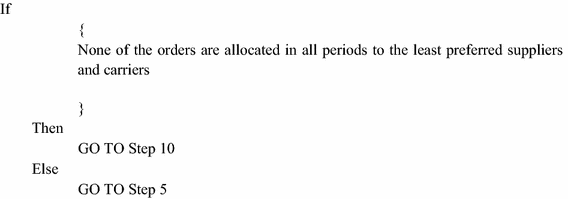
• Step 10: Flexible dynamic sustainable procurement (FDSP) is obtained.

  FDSP solution will ensure the minimum order allocation of all parts in all periods to the least preferred suppliers and carriers.

5 Case illustration

The section demonstrates the proposed FDSP model through a case illustration. The procurement problem for a manufacturing firm is considered for three time periods for ten different parts to be ordered from six different suppliers each using five various carriers. The buying firm identifies the most preferred and least preferred set of suppliers and carriers among the available ones. The firm models the dynamic procurement problem where demand of all the parts is known and suppliers and carriers have limited capacity. The parameters are known and dynamic. One or more carrier types can be used by suppliers for transporting the ordered parts to the manufacturing firm. Firm minimizes the total procurement cost including raw material cost, ordering cost, transportation cost, holding cost and carbon emissions cost over the entire planning horizon. The carbon emissions are considered for the process of ordering, holding and transportation. The DSP model establishes an optimal trade-off between costs incurred and emissions caused in procurement process. However, it is required for the firm to minimize the order allocations made to the least preferred set of suppliers and carriers to prevent supply chain disruptions. Excluding the least preferred suppliers and carriers might result in increased procurement cost and possible infeasibility due to insufficient capacities by other suppliers. Therefore, a necessary trade-off must be established. The data for problem in terms of demand, carrier capacity and supplier capacity is tabulated in Appendix B.

5.1 Phase-I: qualitative models

5.1.1 Qualitative model for supplier selection

The set of criteria for selection of suppliers are considered for the manufacturing firm and relative weightages of criteria are evaluated using DEMATEL. Table 2 shows the list of criteria considered and the weightage corresponding to each criterion. The procedure for criteria identification and selection can be referred from Kaur et al. (2016). Based on these criteria the six suppliers are ranked using AHP, TOPSIS, IRP, W-IRP and BAK and the final ranking is derived using ILP. The Final supplier rankings are shown in Table 3, from where it can be seen that least preferred suppliers are $\hbox {S}_{1}$ and $\hbox {S}_{2}$, whereas $\hbox {S}_{4}$ and $\hbox {S}_{3}$ are most preferred suppliers .

Table 2 List of criteria and criteria weights derived using DEMATEL (Kaur et al. 2016)

Table 3 Final supplier ranking

5.1.2 Qualitative model for carrier selection

The criteria for carrier selection are considered with the help of published literature (Vijayvargiya and Dey 2010; Yang and Regan 2013; Basu et al. 2016) and industry experts. The expert opinions are then used to derive criteria weights using DEMATEL. The list of criteria and corresponding weightages are provided in Table 4. The available 5 types of carriers namely- truck $(\hbox {M}_{1})$, open trailer $(\hbox {M}_{2})$, trailer $(\hbox {M}_{3})$, long haul $(\hbox {M}_{4})$ and high cube $(\hbox {M}_{5})$ are ranked based on these set of criteria using MCDM techniques such as AHP, TOPSIS, IRP, W-IRP and BAK. The responses of industry experts and interaction matrices for DEMATEL and other MCDM techniques are shown in Appendix (Tables 12, 13, 14, 15, 16, 17). The various ranks obtained are integrated using ILP. The ranks obtained are shown in Table 5. It can be observed from the Table 5 that carriers $\hbox {M}_{1 }$ and $\hbox {M}_{2}$ are least preferred whereas carriers $\hbox {M}_{4}$ and $\hbox {M}_{5}$ are most preferred carriers .

Table 4 List of criteria for carrier selection and corresponding weightages derived using DEMATEL

Table 5 Final carrier ranking

5.2 Phase-II: dynamic sustainable procurement (DSP) model

DSP is solved for three periods, ten parts procurement problem using six suppliers and five carriers. The model provides optimal solution in terms of lot-sizing, supplier selection and carrier selection optimizing total procurement cost comprising of raw material cost, ordering cost, transportation cost, holding cost and carbon emissions cost. Complete solution demonstrating allocations for each product to each supplier as well as each carrier is shown in Table 6. The italic cells shows the allocations made either to least preferred supplier or carrier. These allocations are observed as the model is purely based on quantitative parameters and does not include qualitative preferences of the firm. This limitation is overcome using FDSP model illustrated in Sect. 5.3.

Table 6 Optimal solution of DSP model

5.3 Phase-III: flexible dynamic sustainable (FDSP) model

The proposed FDSP model integrates the qualitative and quantitative models. It is observed from quantitative model solution, orders are allocated to the least preferred suppliers and carriers, due to low cost. However, in real practice, order allocation to least preferred suppliers and carriers are discouraged as it might lead to late deliveries, unreliability and quality issues. On the other hand, order allocations to highly preferred suppliers are encouraged to ensure reliability. Hence, there is a need to consider solutions obtained from qualitative and quantitative models together for an effective and efficient procurement. This need is addressed in the proposed FDSP model using following steps.

• Step 1: Solve qualitative model for suppliers

  Suppliers are ranked through the qualitative model explained in Sect. 5.1.1. Results are shown in Table 3.

  • Step 1.1: Identify the set of most preferred suppliers

    From Table 3, the most preferred set of suppliers is given below. Here, best two suppliers are considered as the most preferred suppliers.

    $$\begin{aligned} \mathbf{Most }\,\mathbf{preferred }\,\mathbf{suppliers: } \left\{ \mathbf{S}_{\mathbf{3}} , \mathbf{S}_{\mathbf{4}}\right\} \end{aligned}$$

  • Step 1.2: Identify the set of least preferred suppliers

    Similarly, set of least preferred suppliers from Table 3 is shown below. Here, last two suppliers are considered as the least preferred suppliers.

    $$\begin{aligned} \mathbf{Least }\,\mathbf{preferred }\,\mathbf{suppliers: } \left\{ \mathbf{S}_{\mathbf{1}} , \mathbf{S}_{\mathbf{2}}\right\} \end{aligned}$$

• Step 2: Solve qualitative model for carriers

  Carriers are ranked through the qualitative model explained in Sect. 5.1.2. Results are shown in Table 5.

  • Step 2.1: Identify the set of most preferred carriers

    From Table 5, the set of most preferred carriers is given below. Here, top two carrier types are considered as the most preferred carriers.

    $$\begin{aligned} \mathbf{Most }\,\mathbf{preferred }\,\mathbf{carriers: }\left\{ \mathbf{M}_{\mathbf{4}}, \mathbf{M}_{\mathbf{5}}\right\} \end{aligned}$$

  • Step 2.2: Identify the set of least preferred carriers

    Similarly, the set of least preferred carriers from Table 5 is shown below. Here, last two carrier types are considered as the least preferred carriers.

    $$\begin{aligned} \mathbf{Least }\,\mathbf{preferred }\, \mathbf{carriers: }\left\{ \mathbf{M}_{\mathbf{1}}, \mathbf{M}_{\mathbf{2}}\right\} \end{aligned}$$

• Step 3: Solve quantitative model for DSP

  The quantitative model for DSP shown in Sect. 4.2 is solved (refer Sect. 5.2). The optimal solution obtained for DSP is shown in Table 6.

• Step 4: Compare the solution obtained at step 3 with step 1 and step 2

  The optimal solution of DSP is compared with the set of least preferred suppliers (from Step 1) and least preferred carrier types (from Step 2). It is found that the order allocations are made to least preferred suppliers and carriers in some of the time periods. The allocations made to least preferred suppliers and carriers are shown as italic cells in Table 6 and are shown here (Total forty allocations are made to least preferred suppliers and carriers).

  Table 7 Possible elimination strategies to formulate FDSP

  $$\begin{aligned} \left\{ {\begin{array}{ccccc} X_{(1, 1, 1, 5)} =230&{}X_{(2, 1, 2, 5)} =100&{}X_{(2, 1, 6, 2)} =220&{}X_{(3, 1, 3, 2)} =260&{}X_{(1, 2, 1, 5)} =130 \\ X_{(1, 2, 2, 5)} =230&{}X_{(2, 2, 2, 5)} =100&{}X_{(3, 2, 2, 5)} =170&{}X_{(1, 3, 1, 5)} =190&{}X_{(2, 3, 3, 2)} =220 \\ X_{(1, 4, 1, 5)} =160&{}X_{(1, 4, 2, 5)} =150&{}X_{(2, 4, 1, 4)} =230&{}X_{(3, 4, 2, 5)} =190&{}X_{(2, 5, 1, 4)} =170 \\ X_{(2, 5, 2, 5)} =210&{}X_{(3, 5, 2, 5)} =140&{}X_{(2, 6, 2, 5)} =120&{}X_{(3, 6, 1, 5)} =200&{}X_{(2, 7, 2, 5)} =150 \\ X_{(2, 7, 3, 2)} =130&{}X_{(1, 7, 2, 5)} =280&{}X_{(3, 7, 6, 2)} =190&{}X_{(1, 8, 1, 5)} =290&{}X_{(1, 8, 2, 5)} =180 \\ X_{(1, 8, 3, 2)} =200&{}X_{(2, 8, 2, 5)} =280&{}X_{(3, 8, 2, 5)} =290&{}X_{(3, 8, 6, 2)} =160&{}X_{(1, 9, 1, 4)} =210 \\ X_{(1, 9, 2, 2)} =160&{}X_{(2, 9, 1, 4)} =220&{}X_{(2, 9, 3, 2)} =250&{}X_{(3, 9, 1, 5)} =140&{}X_{(3, 9, 4, 5)} =150 \\ X_{(1, 10, 2, 5)} =160&{}X_{(1, 10, 3, 2)} =290&{}X_{(2, 10, 1, 4)} =130&{}X_{(3, 10, 2, 5)} =210&{}X_{(3, 10, 6, 2)} =230 \\ \end{array}}\right\} \end{aligned}$$

  Since forty allocations are made to least preferred suppliers and carriers, so, GO TO Step 5.

• Step 5: Construct elimination strategies

  Elimination strategies are constructed considering least preferred suppliers and carriers from step 1 and step 2. The elimination strategies are constructed such that no allocation to be made to the least preferred combination of suppliers and carriers in few or all periods. Table 7 shows all the possible combination of elimination strategies considering all nine possible combination of least preferred suppliers and carriers $\{\hbox {S}_{1}\hbox {M}_{1}, \hbox {S}_{2}\hbox {M}_{2}, \hbox {S}_{1}\hbox {M}_{2,}, \hbox {S}_{2}\hbox {M}_{1,}, \hbox {S}_{1}\hbox {S}_{2}\hbox {M}_{1,}, \hbox {S}_{1}\hbox {S}_{2}\hbox {M}_{2,},\hbox {M}_{1}\hbox {M}_{2}\hbox {S}_{1}, \hbox {M}_{1}\hbox {M}_{2}\hbox {S}_{2,}, \hbox {S}_{1}\hbox {S}_{2}\hbox {M}_{1}\hbox {M}_{2}\}$ for all possible combination of the time periods $\{\hbox {T}_{1}, \hbox {T}_{2}, \hbox {T}_{3}, \hbox {T}_{1} \hbox {T}_{2}, \hbox {T}_{1}\hbox {T}_{3}, \hbox {T}_{2}\hbox {T}_{3}, \hbox {T}_{1}\hbox {T}_{2}\hbox {T}_{3}\}$. A total of sixty-three possible elimination strategies are constructed and shown in Table 7. Each cell of Table 7 shows respective constraint generated from the corresponding the corresponding elimination strategies.

• Step 6: Formulate FDSP

  FDSP is formulated by adding elimination strategy constructed at step 5 and the DSP formulation described at Sect. 4.2 A total of sixty-three models would be formulated. The generic formulation of FDSP by adding elimination strategy is shown here.

  Objective function

  $$\begin{aligned} \begin{array}{lll} \hbox {Minimize}&\quad \hbox {Equation}&(1) \end{array} \end{aligned}$$

  Subject to

  $$\begin{aligned} \begin{array}{lll} &{}\hbox {Equations} &{}\quad (2{-}11)\\ &{}\hbox {Elimination strategy} &{}\quad (12)\\ \end{array} \end{aligned}$$

  For instance, elimination strategy to prevent order allocation to $\hbox {S}_{1}\hbox {M}_{1}$ for period $\hbox {T}_{1}$ would be written as equation (12) which is given below.

  $$\begin{aligned} U_{1i11}=0 \qquad \forall i \end{aligned}$$

  (12)

  Similarly, all sixty-three elimination strategies would be considered for FDSP.

• Step 7: Solve FDSP

  The FDSP formulated at step 6 is solved optimally for all elimination strategies. The objective function value of optimal solution for all sixty-three FDSP models corresponding to all sixty three elimination strategies are shown in table 8. Some of the FDSP for corresponding elimination strategies fails to give feasible solution and are also shown in Table 8.

• Step 8: Generate deviation matrix

  Percentage deviation is calculated from objective function value of DSP model obtained at step 3 and objective function value of sixty-three FDSP obtained at step 7 for all elimination strategies. Table 9 shows percentage deviational.

• Step 9: Construct Flexible Dynamic Sustainable Procurement (FDSP) decision

  Table 8 Objective function value of FDSP considering all elimination strategies

  FDSP decision would be based on the percentage deviation of FDSP model calculated at step 8 and the percentage deviation acceptable to the procuring firm. For an instance, if the procuring firm accepts deviation upto 5% the solution obtained using elimination strategy corresponding to deviation of 4.69% can be considered as the best suitable procurement decision. Table 10 shows order allocation by FDSP model with deviation of 4.69%. The FDSP solution restricts allocating orders to the least preferred suppliers ($\hbox {S}_{1}$ and $\hbox {S}_{2}$) and carriers ($\hbox {M}_{1}$ and $\hbox {M}_{2}$) for time period $\hbox {T}_{2}$ and $\hbox {T}_{3}$ respectively, however, it is being allowed for $\hbox {T}_{1}$. It can be further seen from Table 8 that avoiding all least preferred suppliers and carriers across entire period is not possible due to constraint violation and hence, fails to give feasible solution. Therefore, the sustainable procurement has to be flexible in deciding the most appropriate sustainable procurement decision to avoid maximum possible least preferred suppliers and carriers. In the given flexible sustainable procurement with 4.69% deviation, it can be seen that the least preferred suppliers and carriers are not allocated in time period $\hbox {T}_{2}$ and $\hbox {T}_{3}$.

  Table 11 presents order allocation to suppliers and carriers of DSP and proposed FDSP models. Table 11 also provides detailed comparison of lot-sizing, order allocation to suppliers and carriers from DSP and FDSP model. From the Table 11, it can be seen that allocation to the least preferred suppliers and/or carriers (shown in bold) is minimized using FDSP model.

• Step 10: Flexible dynamic sustainable procurement (FDSP) is obtained.

  For the given acceptable % deviation, the FDSP decision is obtained and ensure the minimum order allocation of all parts in all periods to the least preferred suppliers and carriers. The details of FDSP solution is shown in Table 11.

Table 9 Percentage deviational for FDSP

Table 10 FDSP optimal solution corresponding to 4.69% deviation

Table 11 Comparison between order allocation of DSP and FDSP

6 Managerial insights, contributions, and limitations

The section discusses the managerial insights, contributions and limitations of the proposed FDSP framework.

6.1 Managerial insights

• The proposed FDSP model allows incorporating and integrating the qualitative preferences for suppliers and carriers in the quantitative modelling to minimize order allocation to the least preferred suppliers and carriers.

• The proposed framework provides the procurement managers with a number of possible elimination strategies to avoid allocation to least preferred supplier and carrier. Hence, the buying firm can select the best suited strategy for sustainable managers can choose the strategy which works best for their firm.

6.2 Contributions

• The paper proposes the qualitative modelling for suppliers and carriers using various MCDM techniques such as AHP, TOPSIS, IRP, W-IRP and BAK integrating these ranks to derive final ranks through an integer linear program.

• The paper proposes a flexible dynamic sustainable procurement (FDSP) framework, which is an integration of various qualitative models (AHP, TOPSIS, IRP, W-IRP and BAK) and a quantitative model (i.e. DSP) in procurement.

• The proposed FDSP framework provides an approach for sustainable procurement. The FDSP model modifies the procurement solution obtained from quantitative model (i.e. DSP) by incorporating qualitative preferences through qualitative model.

6.3 Limitations

• The proposed FDSP framework considers deterministic data for qualitative and quantitative model.

• The proposed FDSP framework is currently limited to AHP, TOPSIS, IRP, W-IRP and BAK approaches for suppliers and carrier ranking.

7 Conclusions and future scope of work

The paper models FDSP by integrating qualitative and quantitative model. Qualitative models such as AHP, TOPSIS, IRP, W-IRP, BAK and ILP are applied for identifying the most preferred and least preferred set of suppliers and carriers. Quantitative model (i.e. DSP) is optimally solved for multi-part, multi-period procurement problem involving multiple suppliers and carriers. The DSP being cost based model tend to allocate orders to suppliers and carriers offering least cost but on the other hand these are least preferred by the firm. This creates contradiction between DSP and qualitative model. To avoid such contradiction, a flexible dynamic sustainable procurement (FDSP) framework is proposed which minimizes the difference in solution of quantitative model (i.e. DSP) and quantitative models. The proposed FDSP minimizes the order allocation in procurement problem to the least preferred suppliers and carriers in the most flexible and sustainable way demonstrated through an illustration. The proposed FDSP can be extended in future for stochastic and uncertain data. The proposed FDSP can be also extended for fuzzy parameters. In addition more MCDM techniques such as PROMETHEE, ELECTREE and VICKOR can also be applied to rank suppliers and carriers.

Appendices

Appendix A

See Tables 12, 13, 14, 15, 16 and 17.

Table 12 Mode of DEMATEL responses obtained for carrier criteria

Table 13 Pair-wise comparison matrices between carriers for all criteria (AHP)

Table 14 Comparison matrix for TOPSIS

Table 15 Dominating interaction matrix (IRP and W-IRP)

Table 16 Calculation of Net Dominance for carriers using IRP

Table 17 Calculation of Net Dominance for carriers using W-IRP

Appendix B

See Table 18.

Table 18 Data set for (3T-10P-6S-5M) problem

References

Aggarwal, R., & Singh, S. P. (2015). Chance constraint-based multi-objective stochastic model for supplier selection. The International Journal of Advanced Manufacturing Technology, 79(9–12), 1707–1719.
Aissaoui, N., Haouari, M., & Hassini, E. (2007). Supplier selection and order lot sizing modeling: A review. Computers & Operations Research, 34, 3516–3540.
Basu, R. J., Subramanian, N., Gunasekaran, A., & Palaniappan, P. L. K. (2016). Influence of non-price and environmental sustainability factors on truckload procurement process. Annals of Operations Research, 1–26. doi:10.1007/s10479-016-2170-z.
Benjaafar, S., Li, Y., & Daskin, M. (2013). Carbon footprint and the management of supply chains: Insights from simple models. IEEE Transactions on Automation Science and Engineering, 10(1), 99–116.
Bonney, M., & Jaber, M. Y. (2011). Environmentally responsible inventory models: Non-classical models for a non-classical era. International Journal of Production Economics, 133, 43–53.
Bouchery, Y., Ghaffari, A., Jemai, Z., & Dallery, Y. (2012). Including sustainability criteria into inventory models. European Journal of Operational Research, 222, 229–240.
Chan, F. T. S., Kumar, N., Tiwari, M. K., Lau, H. C. W., & Choy, K. L. (2008). Global supplier selection: A fuzzy-AHP approach. International Journal of Production Research, 46(14), 3825–3857.
Chen, C. T., Lin, C. T., & Huang, S. F. (2006). A fuzzy approach for supplier evaluation and selection in supply chain management. International Journal of Production Economics, 102, 289–301.
Chen, F., Federgruen, A., & Zheng, Y. S. (2001). Coordination mechanisms for a distribution system with one supplier and multiple retailers. Management Science, 47(5), 693–708.
Chiang, W. C., & Russell, R. A. (2004). Integrating purchasing and routing in a propane gas supply chain. European Journal of Operational Research, 154(3), 710–729.
Cholette, S., & Venkat, K. (2009). The energy and carbon intensity of wine distribution: A study of logistical options for delivering wine to consumers. Journal of Cleaner Production, 17(6), 1401–1413.
Choudhary, D., & Shankar, R. (2013). Joint decision of procurement lot-size, supplier selection, and carrier selection. Journal of Purchasing and Supply Management, 19(1), 16–26.
Choudhary, D., & Shankar, R. (2014). A goal programming model for joint decision making of inventory lot-size, supplier selection and carrier selection. Computers & Industrial Engineering, 71, 1–9.
Cook, W. D., & Seiford, L. M. (1982). On the Borda–Kendall consensus method for priority ranking problems. Management Science, 28(6), 621–637.
De Boer, L., Labro, E., & Morlacchi, P. (2001). A review of methods supporting supplier selection. European journal of purchasing & supply management, 7(2), 75–89.
Fraering, M., & Prasad, S. (1999). International sourcing and logistics: An integrated model. Logistics Information Management, 12(6), 451–460.
Gaballa, A. A. (1974). Minimum cost allocation of tenders. Operational Research Quarterly, 25, 389–98.
Ghodsypour, S. H., & O’Brien, C. (1998). A decision support system for supplier selection using an integrated analytic hierarchy process and linear programming. International Journal of Production Economics, 56–57, 199–212.
Ghodsypour, S., & O’Brien, C. (2001). The total cost of logistics in supplier selection, under conditions of multiple sourcing, multiple criteria and capacity constraint. International Journal of Production Economics, 73, 15–27.
Handfield, R., Walton, S. V., Sroufe, R., & Melnyk, S. A. (2002). Applying environmental criteria to supplier assessment: A study in the application of the analytical hierarchy process. European Journal of Operational Research, 141(1), 70–87.
Haq, A. N., & Kannan, G. (2006). Fuzzy analytical hierarchy process for evaluating and selecting a vendor in a supply chain model. International Journal of Advanced Manufacturing Technology, 29, 826–835.
Helmrich, M. R., Van den Heuvel, W., & Wagelm, A. P. (2011). The economic lot-sizing problem with an emission constraint, 2nd international workshop on lot sizing, Istanbul, Turkey (pp. 45–48).
Hsu, C. W., Chen, S. H., & Chiou, C. Y. (2011). A model for carbon management of supplier selection in green supply chain management. In IEEE international conference on industrial engineering and engineering management (IEEM), Singapore (pp. 1247 – 1250).
Hwang, C. L., & Yoon, K. (1981). Multiple criteria decision making. Lecture Notes in Economics and Mathematical Systems, 186, 58–191.
Jaber, M. Y., Glock, C. H., & El Saadany, A. M. (2013). Supply chain coordination with emissions reduction incentives. International Journal of Production Research, 51(1), 69–82.
Jensen, R. E. (1986). Comparison of consensus methods for priority ranking problems. Decision Sciences, 17(2), 195–211.
Kahraman, C., Cebeci, U., & Ulukan, Z. (2003). Multi-criteria supplier selection using fuzzy AHP. Logistics Information Management, 16(6), 382–394.
Kaur, H., & Singh, S. P. (2016). Modelling flexible procurement problem. In Sushil, K. T. Bhal, & S. P. Singh (Eds.), Managing flexibility: people, process, technology and business (pp. 147–170). New Delhi: Springer.
Kaur, H., Singh, S. P., & Glardon, R. (2016). An integer linear program for integrated supplier selection: A sustainable flexible framework. Global Journal of Flexible Systems Management, 17(2), 1–22.
Kelle, P., Al-khateeb, F., & Miller, P. A. (2003). Partnership and negotiation support by joint optimal ordering/setup policies for JIT. International Journal of Production Economics, 81, 431–441.
Kumar R., & Singh S. P. (2015). AHP-IRP: An integrated approach for decision making. International conference on evidence based management 2015 (ICEBM) (pp. 605-612). ISBN: 978-93984935-18-4.
Li, Y., Cai, X., Xu, L., & Yang, W. (2015). Heuristic approach on dynamic lot-sizing model for durable products with end-of-use constraints. Annals of Operations Research, 242, 265–283.
Li, X. (2015). Optimal procurement strategies from suppliers with random yield and all-or-nothing risks. Annals of Operations Research. doi:10.1007/s10479-015-1923-4.
Liao, Z., & Rittscher, J. (2007). Integration of supplier selection, procurement lot sizing and carrier selection under dynamic demand conditions. International Journal of Production Economics, 107, 502–510.
Lin, Y. K., & Yeh, C. T. (2013). Determine the optimal carrier selection for a logistics network based on multi-commodity reliability criterion. International Journal of Systems Science, 44(5), 949–965.
Purohit, A. K., Choudhary, D., & Shankar, R. (2016a). Inventory lot-sizing with supplier selection under non-stationary stochastic demand. International Journal of Production Research, 54(8), 2459–2469.
Purohit, A. K., Shankar, R., Dey, P. K., & Choudhary, A. (2016b). Non-stationary stochastic inventory lot-sizing with emission and service level constraints in a carbon cap-and-trade system. Journal of Cleaner Production, 113, 654–661.
Saaty, T. L. (1980). The analytic hierarchy process. New York: McGraw-Hill.
Shyur, H., & Shih, H. (2006). A hybrid MCDM model for strategic vendor selection. Mathematical and Computer Modelling, 44, 749–761.
Songhori, M. J., Tavana, M., Azadeh, A., & Khakbaz, M. Z. (2011). A supplier selection and order allocation model with multiple transportation alternatives. International Journal of Advanced Manufacturing Technology, 52, 365–376.
Stank, T. P., & Goldsby, T. J. (2000). A framework for transportation decision making in an integrated supply chain. Supply Chain Management: An International Journal, 5(2), 71–78.
Sushil (2009). Interpretive ranking process. Global Journal of Flexible Systems Management, 10(4), 1–10.
Swenseth, S. R., & Godfrey, M. R. (2002). Incorporating transportation costs into inventory replenishment decisions. International Journal of Production Economics, 77(2), 113–130.
Tsiakis, P., Shah, N., & Pantelides, C. C. (2001). Design of multi-echelon supply chain networks under demand uncertainty. Industrial & Engineering Chemistry Research, 40(16), 3585–3604.
Ubeda, S., Arcelus, F. J., & Faulin, J. (2011). Green logistics at Eroski: A case study. International Journal of Production Economics, 131(1), 44–51.
Venkat, K. (2007). Analyzing and optimizing the environmental performance of supply chains. Proceedings of the ACCEE summer study on energy efficiency in industry, White Plains, New York, USA.
Vijayvargiya, A., & Dey, A. K. (2010). An analytical approach for selection of a logistics provider. Management Decision, 48(3), 403–418.
Wagner, H. M., & Whitin, T. M. (1958). Dynamic version of the economic lot size model. Management science, 5(1), 89–96.
Wang, G., Samuel, H. H., & Dismukes, J. P. (2004). Product-driven supply chain selection using integrated multi-criteria decision-making methodology. International Journal of Production Economics, 91, 1–15.
Ware, N. R., Singh, S. P., & Banwet, D. K. (2014b). A mixed-integer non-linear program to model dynamic supplier selection problem. Expert System With Applications, 41, 671–678.
Ware, N. R., Singh, S. P., & Banwet, D. K. (2014a). Modeling flexible supplier selection framework. Global Journal of Flexible Systems Management, 15(3), 261–274.
Xia, W., & Wu, Z. (2007). Supplier selection with multiple criteria in volume discount environments. Omega, 35, 494–504.
Yang, C. H., & Regan, A. C. (2013). A multi-criteria decision support methodology for implementing truck operation strategies. Transportation, 40(3), 713–728.
Author information
Authors and Affiliations
Corresponding author