
Abstract
This paper considers a two-stage supply chain in which a supplier serves a set of stores in a retail chain. We consider a two-stage Stackelberg game in which the supplier must set price discounts for each period of a finite planning horizon under uncertainty in retail-store demand. As a mechanism to stimulate sales, the supplier offers periodic off-invoice price discounts to the retail chain. Based on the price discounts offered by the supplier, and after store demand uncertainty is resolved, the retail chain determines individual store order quantities in each period. Because the supplier offers store-specific prices, the retailer may ship inventory between stores, a practice known as diverting. We demonstrate that, despite the resulting bullwhip effect and associated costs, a carefully designed price promotion scheme can improve the supplier’s profit when compared to the case of everyday low pricing (EDLP). We model this problem as a stochastic bilevel optimization problem with a bilinear objective at each level and with linear constraints. We provide an exact solution method based on a Reformulation-Linearization Technique (RLT). In addition, we compare our solution approach with a widely used heuristic and another exact solution method developed by Al-Khayyal (Eur. J. Oper. Res. 60(3):306–314, 1992) in order to benchmark its quality.
1 Introduction
Trade promotions, a common practice in consumer packaged goods sectors, involve suppliers who offer temporary price cuts to retailers in the hope that retailers will in turn discount or promote their product to consumers. Trade promotions have long played an important role in U.S. retail supply chains. Use of trade promotions by suppliers of consumer packaged goods to distributors rose from $8 billion in 1990 to approximately $80 billion in 2004 (Gómez et al. 2007). With the lion’s share (52 %) (Ailawadi et al. 1999) of the money spent on advertising and promotions going to trade rather than consumer promotions, 85 % of suppliers believe that their trade promotion dollars are not being spent effectively (Knowledge@Wharton 2001), and only 19 % think they get a good value for their money (Bell and Drèze 2002).
Adoption of “off-invoice” deals is one of the major reasons for the poor performance of trade promotions. In an “off-invoice” trade promotion, a supplier simply deducts some percentage from the invoice price for purchases over a set of periods. Thus, suppliers have no control over whether retailers will actually pass their promotional prices on to end consumers. In fact, a survey shows that, on average, retailers only pass 60 % of trade funds to consumers (Besanko et al. 2005). There are two retailer strategies that reduce the effectiveness of trade promotions. First, retailers may respond to an off-invoice trade promotion by engaging in forward-buying, i.e., the retailer takes advantage of the suppliers’s temporary discount by purchasing a quantity that far exceeds its current needs, and subsequently only applies a discount to part of this order when selling to consumers. When the promotion period expires, the retailer sells the remaining inventory that it purchased at a discount to its consumers at the regular price. Second, retailers may take advantage of off-invoice trade promotions by engaging in diverting, i.e., ordering from one store and redirecting the shipment to another store.
Bronnenberg et al. (2007) show that geographic variation in brand shares for leading consumer brands is both substantial and persistent. Consequently, the marginal effectiveness of promotions and prices varies considerably among retail stores from around the country (Bronnenberg et al. 2005). To accommodate geographic differences in sales of similar products, suppliers may offer certain off-invoice trade promotions only in certain regions of the country. Large national retail chains may circumvent these restrictions by purchasing a product at a lower wholesale price where the deal is offered, and subsequently shipping the item to stores in other regions (where the deal is not offered) for sale at the regular price. Conventional wisdom holds that 5 % to 10 % of grocery products on promotion are diverted (Berry 1992).
These forward-buying and diverting strategies make the retailer’s store order pattern differ from the store’s consumer demand pattern, and consequently the variation in a retailer’s order quantity may be much larger than the variation in end-consumer demand. This resulting phenomenon is known as the bullwhip effect, which is viewed in extremely negative terms because of its negative impacts on supply chain operations costs. Moreover, Lee et al. (1997) characterized price variations as one of the major causes of the bullwhip effect. Consequently, in order to reduce the operations costs associated with the bullwhip effect, in March 1997, Procter & Gamble announced plans to eliminate 20 % of its brands from trade promotion contracts; other major suppliers also began to adopt corresponding management practices (an EDLP strategy, for example) to stabilize prices. However, a recent survey conducted by MEI Computer Technology Group Inc. showed that 42 % of the respondents, consisting of consumer packaged goods (CPG) suppliers, said they would spend more on trade promotions in 2010 than ever before (MEI 2010). These suppliers continue to offer trade promotions for several reasons. First, a trend exists in the packaged goods industry in which power is shifting towards retailers and away from suppliers, and this increasing power shift has led retailers to pursue higher rewards. Second, two-thirds of all consumer purchase decisions are made in retail stores (Murry and Heide 1998), and 40 % of consumers look for deals at retail stores (Miller 1997). However, some retailers are reluctant to offer sales promotions unless suppliers fund promotions, at least to some extent, because the retailer’s promotion of one brand may cannibalize sales of a competing brand in the same store, which may reduce the retailer’s total profit. As a result, systemic inefficiencies associated with trade promotions along with pressure applied by powerful retailers lead to a substantial dilemma for suppliers.
In this study, we develop a decision model for designing a supplier’s trade promotion scheme by taking the retailer’s anticipated reactions into consideration. Our model captures a degree of information asymmetry between the supplier and retailers at a coarse level. In particular, because retail stores are in local markets, this provides the retail chain with much better information regarding future demand than is available to the supplier. In many cases retail chains are reluctant to share past demand realizations and future demand forecasts with suppliers in order to prevent this information from reaching competitors. As a result, retailers often have access to much more precise demand information than suppliers (in certain cases the retailer may even make-to-order, implying that its demand is known at the time it places orders with the supplier). We model this asymmetry by assuming that the retailer is able to precisely forecast future demands in the short run, while from the supplier’s perspective, end-consumer demand in each period at every store is uncertain. Thus, the supplier must create its plan for a stochastic demand sequence while the planning problem from the retailer’s perspective is effectively deterministic.
The remainder of this paper is organized as follows. The next section summarizes the related literature. Section 3 then describes our supply chain model. We present three approaches for solving the resulting problem in Sect. 4. We first transform our original model to a generalized bilinear programming problem in Sects. 4.1 and 4.2. Section 4.3.1 presents a widely used heuristic solution method previously developed for solving bilinear problems, followed by Sects. 4.3.2 and 4.3.3, which present two exact solution methods. The first of these is a modification of Al-Khayyal’s approach (Al-Khayyal 1992) for solving generalized bilinear programs and the second is a new approach we have developed for this problem class. In Sect. 5, we discuss the results of a computational study used to validate our solution method and compare it with the results of the heuristic method and Al-Khayyal’s approach. We conclude in Sect. 6 with a discussion of the insights provided by our results.
2 Literature review
A study by Andersen Consulting (Drèze and Bell 2003) found that “trade promotion is the biggest, most complex and controversial dilemma facing the retail industry today.” Despite the many undesirable consequences discussed in the operations literature, there has been no sign of decline in the use of trade promotions in industry. Ailawadi et al. (1999) used a numerical example to demonstrate that a well-designed off-invoice trade promotion can increase both the total supply chain system’s profits and the upstream player’s profits. Blattberg et al. (1981) suggested that effective timing of off-invoice trade promotions can reduce a supplier’s inventory cost. Drèze and Bell (2003) showed that scan-back trade promotions may improve both the retailer’s and the supplier’s performance. Scan-back trade promotions are so named because they are based on stores’ scanner data and, therefore, the amount sold to end consumers from each store.
Studying the effects of trade promotions in a supply chain requires a model that simultaneously considers pricing and operations decisions. The integration of pricing with inventory and distribution decisions over a finite planning horizon has been widely studied in the literature for a single firm within a supply chain. Under the assumption of deterministic demand, Ardalan (1991, 1994) developed a model that determines both the retailer’s optimal price and ordering policies in response to a one-time only price discount using a general price-demand relationship. Arcelus and Srinivasan (1998) generalized this work by accounting for potential forward buying at the retailer. For the more general case in which price discounts can be offered on more than one occasion, Sogomonian and Tang (1993) developed a model that determines optimal promotion and production decisions for a single profit-maximizing firm using mixed-integer programming. Based on the assumptions that promotion levels belong to a finite set and the consumer response to promotions depends on the time elapsed since the last promotion, they proposed an approach to solve the problem globally by reformulating their problem as a “longest path” problem on a network. Su and Geunes (2012) provided a deterministic two-echelon supply chain model in which the supplier’s and retailer’s prices are periodically reduced in conjunction with a promotion. They demonstrated that increased system profit can coexist with the bullwhip effect as a result of trade promotions if the supplier judiciously applies a trade promotion strategy under certain conditions (e.g., a sufficient number of impulsive consumers and/or a low degree of consumer forward buying).
Under the assumption of stochastic demand, Petruzzi and Dada (1999) considered a price-setting firm that stocks a single product subject to random, price-dependent demand, with the objective of determining stock levels over multiple periods. They developed a condition under which the solution to this problem is stationary and myopic. One limitation of their research is the imposition of a constant price assumption. For a joint pricing and inventory management problem with stochastic demand (in which prices may change dynamically over time), Thowsen (1975) showed that the optimal pricing/inventory policy is a base-stock list-price policy under the assumptions that: (i) the expected demand curve and stockout costs are linear functions; (ii) holding costs are convex; and (iii) the density function of the random component of consumer demand is PF 2 (a Pólya frequency function of order 2). Cheng and Sethi (1999) used a Markov decision process (MDP) model for a joint inventory and promotion decision problem in which the promotion has only two states (on and off). Under certain conditions, they showed that the optimal promotion and ordering policy is an (S 0,S 1,P) policy. That is, if the initial inventory level is at least P, the product is promoted; if the initial inventory is less than S 1 and the product is promoted, an order is placed to increase the inventory position to S 1; if the initial inventory is less than S 0 and if the product is not promoted, an order is placed to increase the inventory position to S 0. Additional works that consider the use of pricing and promotions to manage demand in supply chains include Desai (1992), who considers how channel structure affects pricing decisions, Upasani and Uzsoy (2008), who provide a review of lead time and pricing decision models, and Xiao et al. (2005), who consider promotions and supply chain contract parameters with demand disruptions.
In this paper, we provide a mathematical model of a decentralized two-echelon supply chain in which the supplier’s pricing decisions (trade promotion levels) and the retailer’s operations decisions (order quantities, inventory levels, and transshipment quantities) are determined simultaneously. To broaden the applicability of our model, we assume that the price can be dynamically changed over time and that demand is stochastic and price-dependent. To the best of our knowledge, no existing work considers an exact solution method for a joint promotion and operations problem in a multi-echelon supply chain under uncertain demand, as we do in this paper. Neslin et al. (1995) developed a multi-echelon model the considers the actions of a supplier, retailer, and consumers from the point of view of the supplier who attempts to maximize profit by targeting advertising to consumers and trade promotions to retailers. However, they do not provide a procedure for obtaining a globally optimal solution. Moreover, their modeling approach parameterized on all of the retailer’s decisions, which effectively leads to a single-level model, whereas our model explicitly considers two separate decision-making units, i.e., a supplier and a retailer. In the field of mathematical programming, this problem falls in the class of linearly constrained, bilevel, nonconvex optimization problems. Most of the available algorithms in the field of bilevel programming apply to bilevel linear problems (where, for fixed values of one set of decision variables, the remaining problem becomes a linear program). Ben-Ayed (1993) and Wen and Hsu (1991) provided detailed reviews of bilevel linear programming problems. They presented a basic model along with characterizations of optimal solution properties for the problem class and some existing solution approaches. To solve linearly constrained bilevel convex quadratic problems, Muu and Van Quy (2003) developed a branch-and-bound algorithm for finding a global optimal solution. As we will see, none of the previously mentioned solution methods for bilinear optimization problems can be directly applied to the model we develop, which falls within a more general class of nonconvex bilevel optimization problems. These methods have, however, provided substantial guidance and inspiration for the solution procedure we have developed for solving the problem we define.
As we later discuss, our model can be cast as a generalized bilinear program (GBP). Al-Khayyal (1992) provided a generic approach for solving GBPs globally; this approach was essentially an extension to the Al-Khayyal and Falk (1983) algorithm which was proposed to solve jointly constrained bilinear programs. Al-Khayyal et al. (1995) further extended the applicability of this method to nonconvex quadratically constrained quadratic programs. Our solution approach adapts the branch-and-bound algorithm of Al-Khayyal (1992) and also draws on previously developed Reformulation-Linearization (RLT) techniques. Sherali and Alameddine (1992) developed a branch-and-bound algorithm based on an RLT for jointly constrained bilinear programs. Although the linear relaxation obtained from the RLT approach is theoretically tighter than that derived by AI-Khayyal’s method, this RLT branch-and-bound approach cannot be applied to GBPs directly. In our study, we develop a method which is able to solve our problem by integrating the RLT branch-and-bound algorithm within a penalty-function-based approach, which penalizes violations of a relaxed constraint set in the objective function.
3 Problem definition and formulation
To formalize our model, we define the following notation:
- i,j::
-
retail store indices, i,j=1,…,S.
- l::
-
period index, l=1,…,L.
- L P::
-
number of periods in the supplier’s promotion time window, 1<L P<L.
- \(c_{i}^{l}\)::
-
supplier’s initial unit wholesale price for store i in period l.
- \(m_{i}^{l}\)::
-
supplier’s unit production and transportation cost for retail store i in period l.
- \(h_{i}^{l}\)::
-
retailer’s unit inventory holding cost at store i in period l.
- \(t_{ij}^{l}\)::
-
retailer’s unit transportation cost between stores i and j in period l, where i≠j.
- \(d_{i}^{l}\)::
-
base value of deterministic component of consumer demand at store i in period l.
- \(\alpha_{i}^{l}\)::
-
retailer’s pass-through rate at store i in period l.
- \(\gamma_{i}^{l}\)::
-
consumer promotional price elasticity at store i in period l.
- \(z_{i}^{l}\)::
-
supplier’s price discount at store i in period l.
- \(x_{i}^{l}\)::
-
retailer’s order quantity at store i in period l.
- \(I_{i}^{l}\)::
-
retailer’s inventory level at store i at the end of period l.
- \(y_{ij}^{l}\)::
-
retailer’s transhipment quantity from store i to store j in period l.
We consider the following two-echelon system. A make-to-order supplier distributes a single product to a set of retail stores who in turn sell the item to consumers over a finite planning horizon of L periods. The retailer runs a chain of S stores, which serve geographically dispersed, heterogeneous markets, and face random, price-dependent demand at each store.
The supplier and retailer act non-cooperatively and in a sequential manner. The supplier (upper level) selects trade promotion level \(z_{i}^{l}\) targeted at each retail store in each period between period 1 and L P (≤L) in order to maximize its expected profit.Footnote 1 Given the supplier’s price discounts, the retailer (lower level) optimizes its profit by choosing: (1) the order quantity at store i in period l, denoted by \(x_{i}^{l}\); (2) the inventory level at store i at the end of period l, denoted by \(I_{i}^{l}\); and (3) the diverting quantity from store i to store j in period l, denoted by \(y_{ij}^{l}\), for all periods l=1,…,L and all stores i,j=1,…,S, i≠j. The supplier explicitly incorporates the anticipated reactions of the retailer in its optimization process, and we assume full information is available to the supplier regarding the retailer’s inventory and transportation costs. This fits the classical Stackelberg game paradigm, where the leader, who is aware of the follower’s best response, chooses a move that maximizes its own expected payoff.
We assume randomness in demand is price-independent and can be modeled in an additive fashion. Specifically, demand is defined as \(\tilde{d}_{i}^{l}(\omega)=d_{i}^{l} + \alpha_{i}^{l}\gamma_{i}^{l} z_{i}^{l}+ \varepsilon_{i}^{l}(\omega)\), where ω is an outcome belonging to some space Ω, and ω influences all random variables \(\varepsilon_{i}^{l}\). Note that the quantity \(\alpha_{i}^{l} z_{i}^{l}\) is the price discount seen by consumers as it is the product of the retailer’s discount pass-through rate and the supplier’s trade discount. Thus, the quantity \(\alpha_{i}^{l}\gamma_{i}^{l} z_{i}^{l}\) corresponds to the increase in demand at retail store i in period l as a result of the discount passed through to consumers.
As noted in the introduction, we assume that the retailer makes its decisions (\(x_{i}^{l}\), \(I_{i}^{L}\), and \(y_{ij}^{l}\)) after demand uncertainty is resolved but before demand occurs. One interpretation of this assumption is that, from a marketing perspective, retailers are, by definition, closer to consumers than manufacturing companies, and so retailers can more easily engage in personal contact with consumers, gather information on consumer behavior, and anticipate consumer purchase patterns in the short run. And, because retailer resupply lead times are often very short, the retailer has the luxury of placing orders immediately before demand occurs (or even in response to demand in some cases, as in a make-to-order setting). Moreover, effective promotions are usually those offered only over a short time-span, because frequent usage of promotions diminishes their effectiveness (Blattberg and Neslin 1989). As a result, we can often assume that a retailer can accurately forecast consumer demand during promotion periods in the near future. However, we assume that the retailer does not share consumer information with the supplier in this decentralized supply chain. Because the supplier does not possess the retailer’s specialized knowledge of local markets, the supplier cannot accurately forecast consumer demand at the local level; as a result, the supplier must determine its promotional discount levels (\(z_{i}^{l}\) values) for the planning horizon in the absence of precise local demand information. Thus, the asymmetry in the degree of demand uncertainty between the supplier and retailer is attributable to the retailer’s ability to obtain more precise local demand information. From the supplier’s perspective it is either too costly to obtain this local information or the retailer is unwilling to share this information for competitive reasons.
Our model captures the interaction between the supplier and retail chain. The purpose of the model is to determine the optimal promotion plan for the supplier when anticipating the retail chain’s usage of forward buying and diverting strategies. To simplify the exposition of the model and for model tractability, we assume that: (1) replenishment delays are negligible; (2) fixed costs are zero (or constant); (3) transhipment between any two stores can be done within one period; and (4) the retailer’s discount pass-through rates are fixed or pre-determined.Footnote 2 In our model, the supplier makes to order and wishes to maximize its expected net profit. Because of assumption (2) above, the supplier’s expected net profit in any period therefore equals its profit margin (determined by its wholesale price less its marginal cost and discount level) multiplied by the expected demand in the period. The retail chain wishes to meet all of its demand at minimum total cost over the planning horizon.
Based on the above notation and model description, the trade promotion problem can be formulated as a stochastic bilevel program with bilinear objectives at both decision levels, and with linear constraints. For a given realization ω, the order quantity \(x_{i}^{l}(\omega)\), forward buying quantity \(I_{i}^{l}(\omega)\), and diverting quantity \(y_{ij}^{l}(\omega)\) correspond to an optimal solution to the lower level linear program for given upper level trade promotion levels \(z_{i}^{l}\), the optimal values of which are determined by maximizing the expected value of net supplier profit across all possible realizations.
We can now formulate our stochastic multi-period, two-stage trade promotion problem as:
where (x(ω),I(ω),y(ω)) is an optimal solution of the following problem:

where ξ(ω) is a random vector consisting of all random components \(\varepsilon_{i}^{l}(\omega)\), and where each element has expected value zero. The upper level objective (1) is to maximize expected net profit and is expressed as the difference between the sum of revenues arising from wholesale pricing (\(c_{i}^{l}-z_{i}^{l}\)) and the sum of variable costs. The upper level constraints (2) state that the wholesale price discounts \(z_{i}^{l}\) should be nonnegative and less than or equal to the per unit profit margin, \(c_{i}^{l}-m_{i}^{l}\). The upper level constraints (3) state that, after the supplier’s promotion time window, the supplier stops offering a trade promotion to all retail stores, and we add this set of constraints to our model so that it is able to capture the carry-over effect (forward buying, for example) of decisions in promotion periods. The objective of the lower level problem (4) is to minimize the retailer’s total cost of ordering, holding inventory and diverting. In our study, since discount pass-through rates are fixed, it follows that the retail prices are indirectly determined by the supplier. As a result, for the lower level problem, minimizing cost is equivalent to maximizing profit. The first set of lower level constraints (5) requires that ending inventory at store i in period l equals the ending inventory at store i in period l−1, plus the amount ordered from the supplier at store i in period l, plus the amount shipped from other stores to store i in period l−1, minus the demand at store i in period l, minus the amount shipped from store i to other stores in period l. The second set of constraints (6) models consumer demand as a linear function of the wholesale price discount. The remaining constraints indicate that all variables are real-valued and nonnegative.
Note that for a realization ω and specific promotion levels, the objective of the lower level problem is convex (but not strictly convex), which implies the solution to the lower level problem may not necessarily be unique. As a result, we assume that given the choice between solutions to the lower level problem with equal cost, the solution selected is the one yielding the highest expected profit for the supplier. One may alternatively apply a worst-case approach from the supplier’s perspective, assuming that the retailer chooses the solution yielding the lowest expected profit for the supplier.
There are two difficulties inherent in solving STP. First, for each outcome of the demand realization, the resulting problem is a bilevel problem with bilinear objectives at both levels and with linear constraints, which falls in the class of NP-hard bilinearly constrained bilinear programs (or generalized bilinear programs). The second difficulty is the presence of uncertainty in demand: for continuous distributions, exact computation of the expectation involves taking multiple integrals and, in general, implies intractability; for discrete distributions, computing the expectation might involve solving a prohibitively huge number of NP-hard problems.
In the next section, we propose a three step methodology to solve the STP problem globally. First, the stochastic trade promotion problem is converted to an equivalent deterministic problem. Then, we transform the resulting deterministic bilevel problem into a single-level problem. Finally, we adapt a branch-and-bound algorithm based on a Reformulation-Linearization Technique (RLT) for solving the resulting single level generalized bilinear program.
4 Solution procedures for STP
4.1 Deterministic equivalent
In order to analyze the STP, we first construct a time-expanded network G={N,A} representing the two-echelon, multi-period supply chain problem, where N={(i,l):i=1,…,S,l=1,…,L}∪{(0,0)} is the set of nodes and A is the set of arcs. Node (0,0) represents the supplier, while node (i,l) corresponds to retail store i in period l. The set N l={(1,l),(2,l),…,(S,l)}⊂N corresponds to the set of nodes associated with retail stores in period l. Three types of arcs are contained in the network G: (1) ((0,0),(i,l)),∀(i,l)∈N−{(0,0)}, with arc cost \(c_{i}^{l}-z_{i}^{l}\) per unit of flow (order quantity) from the supplier to node (i,l); (2) ((i,l),(i,l+1)),∀(i,l)∈N−N S−{(0,0)} with a unit cost of \(h_{i}^{l}\) corresponding to the inventory carried from node (i,l) to (i,l+1); and (3) ((i,l),(j,l+1)),∀i,j=1,…,S,l=1,…,L−1,i≠j with a unit cost of \(t_{ij}^{l}\) for transshipment from node (i,l) to node (j,l+1).
From the construction of graph G, we might view the lower level problem of STP as a minimum cost flow problem, which requires sending \(\tilde{d}_{i}^{l}(\omega)\) units of flow as cheaply as possible from node (0,0) to each node (i,l) in the set N−{(0,0)} in an uncapacitated network. Observe that a minimum cost flow problem with no arc capacities can be decomposed into a set of S×L shortest path problems that are independent of the demand levels (please see the Appendix for a demonstration of the validity of this decomposition). This observation implies that the lower level problem of STP is equivalent to a set of deterministic problems that are independent of the random terms. Based on this observation, it is not hard to see that for the entire problem, the stochastic components only appear in the objective function of the upper-level problem. After taking the expectation of the objective function, the STP is thus a deterministic problem, and the distributions of the stochastic components do not impact the optimization problem formulation. We next discuss how to transform this deterministic equivalent for the two-level problem into a single-level optimization problem.
4.2 Single-level problem
The deterministic trade promotion problem (DTP) is derived directly from the STP by replacing the random term with its expectation. The results of Sect. 4.1 imply that the DTP is equivalent to STP. Note that the lower level problem can be written without holding costs by making the substitution \(I_{i}^{l}=\sum_{\tau=1}^{l}[x_{i}^{\tau}+\sum_{k\neq i}y_{ki}^{\tau-1}-\sum_{j\neq i }y_{ij}^{\tau}-(d_{i}^{\tau}+\alpha_{i}^{\tau}\gamma_{i}^{\tau}z_{i}^{\tau})]\); then the DTP can be formulated as:
where \(\bar{h}_{i}^{l}=\sum_{\tau=l}^{L} h_{i}^{\tau}\), \(\bar{c}_{i}^{l}=c_{i}^{l}+\bar{h}_{i}^{l}\) and \(\bar{t}_{ij}^{l}=t_{ij}^{l}+\bar{h}_{j}^{l+1}-\bar{h}_{i}^{l}\). For any fixed value of \(z_{i}^{l}\), the lower level problem is a linear program, so any optimal solution of the lower level problem satisfies the strong duality property. As a result, we can replace the lower level program by its primal-dual optimality conditions, where π is the vector of dual variables associated with the set of constraints (7). Let us first define:
and
where \(U^{l}=\sum_{\tau=l}^{L}\sum_{i=1}^{S}(d_{i}^{\tau}+\alpha_{i}^{\tau}\gamma_{i}^{\tau}m_{i}^{\tau})\) and Ω is a hyper-rectangle. Using the above definitions we can formulate the DTP as follows:
The above problem maximizes a bilinear objective function (8) over a feasible region defined by a bilinear constraint (9) and a set of linear constraints. This problem thus falls within the class of generalized bilinear programs (GBPs), and so the SDTP reduces to a linear program whenever either z or (x,y,π) is fixed. However, the objective function (8) and the bilinear constraint (9) are nonconvex functions. Solving a GBP is NP-hard (Petrik and Zilberstein 2011), and, to the best of our knowledge, no methods exist that guarantee convergence to an exact solution in a finite number of steps. In the following section, we will present some classical techniques for solving the SDTP, as well as a penalty-based method that we have developed for solving the problem.
4.3 Linearization
4.3.1 Successive linear programming approach
Successive linear programming is a commonly used heuristic method for solving bilinear programming problems. This procedure iterates between fixing the supplier’s price discounts z and the retailer’s primal and dual variables (x,y,π) for solving the SDTP. At a given iteration k, we first find the values of (x k,y k,π k) that optimize the objective function for a fixed z k−1, and then find the vector z k that optimizes the objective function for fixed values of (x k,y k,π k). We repeat this procedure until the objective does not improve between two successive iterations.
The classical bilinear program is a class of quadratic programs with the following structure:
If the above bilinear program has a finite optimal solution, then there exists an extreme point x ∗∈X and an extreme point y ∗∈Y such that (x ∗,y ∗) is an optimal solution of the classical bilinear program (Vicente et al. 1992). Since the feasible region is defined by two separable polyhedral sets, the classical bilinear program is also called a bilinear program with separable constraints. Sherali and Shetty (1980) showed that, for a classical bilinear program, the limit point of the successive linear programming approach is a locally optimal solution. However, the SDTP is a GBP problem, which does not have separable constraints in the bilinear terms. Therefore, we have no guarantees on solution quality for a solution obtained using the successive linear programming approach.
4.3.2 Al-Khayyal’s approach
Al-Khayyal and Falk (1983) developed an infinitely convergent branch and bound algorithm for jointly constrained bilinear programs (JCBPs) using lower bounds derived from convex envelopes of the bilinear terms. Al-Khayyal (1992) found that the same approach can also be applied for GBPs.
The first step of the approach is to obtain the concave envelope of the objective function (8) over Ω. Piecing together all the variables, we obtain a vector Λ≡(x,y,z,π,η,ζ,ν), with up to N=(5+S+L)×(S×L) components, and the concave envelope of (8) over Ω can be represented as:
where
The second step of the approach is to obtain a polyhedral approximation of the convex hull of the region defined by constraint (9).
By the weak duality theorem, whenever (x,y) and π are feasible for the primal and dual problems, respectively, the left-hand-side of Eq. (9) is always greater than or equal to its right-hand-side. As a result, replacing constraint (9) with the following constraint does not change the feasible region of the SDTP:
Next, define the polyhedral set
Al-Khayyal (1992) showed that for any (x,y,z,π) satisfying constraint (9), there exists Λ∈F 2(Ω).
From the results above, we have the following two observations: (i) ∀(x,y,z,π)∈F∩Ω and Λ∈F∩Ω∩F 1(Ω), we have ϕ(x,y,z,π)≤ψ(Λ); and (ii) for any feasible solution (x,y,z,π) to the SDTP, there exists Λ∈F∩Ω∩F 1(Ω)∩F 2(Ω). Consequently, we have the following convex program for approximating the SDTP:
To solve the SDTP globally, we can implement an infinitely convergent branch-and-bound algorithm based on the above approximation scheme, where partitioning is performed by decomposing Ω into sub-hyper-rectangles. An outline of the algorithm is as follows:
-
Initialization Step: The initial problem is the problem LP(Ω). Initialize Ω (1,1)=Ω and let T 1={(1,1)} be the index set of a single node at iteration one of the branch-and-bound tree. Let UB (1,1)=∞ be the upper bound associated with node (1,1). Let LB=−∞ and UB=∞ be the initial lower and upper bounds of the problem. Set k=1, and go to the Main Step.
-
Main Step: At iteration k, select a node (u,v) from T k and remove this node from T k . Solve LP(Ω (u,v)) to obtain the partial solution \((\bar{x},\bar{y},\bar{z},\bar{\pi})\). If \((\bar{x},\bar{y},\bar{z},\bar{\pi})\) satisfies the constraint (9) and \(\phi(\bar{x},\bar{y},\bar{z},\bar{\pi})=\psi(\bar{\varLambda})\), then the algorithm terminates with \((\bar{x},\bar{y},\bar{z},\bar{\pi})\) as an optimal solution to SDTP(Ω). Otherwise, there are two possible cases: (i) if \((\bar{x},\bar{y},\bar{z},\bar{\pi})\) satisfies constraint (9) but \(\phi(\bar{x},\bar{y},\bar{z},\bar{\pi})<\psi(\bar{\varLambda})\), then let \(LB_{k}=\phi(\bar{x},\bar{y},\bar{z},\bar{\pi})\) be the current iteration lower bound, and set the partitioning index (p,q) as follows:
$$(p,q) = \mathop{\mathrm{arg\,max}}\limits_{(i,l)}\bigl\{ \bar{z}_i^l \bar{x}_i^l-\bar{\eta}_i^l\bigr\} ; $$else (ii) if \((\bar{x},\bar{y},\bar{z},\bar{\pi})\) does not satisfy constraint (9), then let LB k =−∞ be the current iteration lower bound, and set the partitioning index (p,q) as follows:
$$(p,q) = \mathop{\mathrm{arg\,max}}\limits_{(i,l)} \Biggl\{ \max \Biggl[ \bar{c}_i^lx_i^l+\sum _{j\neq i}\bar{t}_{ij}^ly_{ij}^l- \bar{z}_i^l \bar{x}_i^l - \bar{ \zeta}_i^l, -\sum_{\tau=l}^L \bigl(d_i^{l}\bar{\pi}_i^{\tau}+ \alpha_i^l\gamma_i^l \bar{z}_i^l \bar{\pi}_i^{\tau} + \bar{\nu}_i^{l\tau} \bigr) \Biggr] \Biggr\} . $$After finding (p,q), partition the region Ω (u,v) into two mutually exclusive and exhaustive subregions. First, notice that Ω (u,v) is a hyper-rectangle which can be expressed as follows:
$$\varOmega^{(u,v)} \equiv \big\{ (x,y,z,\pi) \in \varOmega: \mathit{ZL}_i^l \leq z_i^l \leq \mathit{ZU}_i^l\quad \forall i=1,\ldots,S,\ l=1,\ldots,L^P \big\} , $$where \(\mathit{ZL}_{i}^{l}\) and \(\mathit{ZU}_{i}^{l}\) are the lower and upper bounds of the component \(z_{i}^{l}\). Using the above notation, the two new subregions can be represented as follows:
$$\begin{aligned} \varOmega^{(k+1,1)} &= \varOmega^{(u,v)}\cap \bigl\{ \mathit{ZL}_p^q \leq z_p^q \leq \bar{z}_p^q\bigr\} \\ \varOmega^{(k+1,2)} & = \varOmega^{(u,v)}\cap \bigl\{ \bar{z}_p^q\leq z_p^q \leq \mathit{ZU}_p^q\bigr\} . \end{aligned}$$Set \(UB^{(k+1,1)}=UB^{(k+1,2)}=\psi(\bar{\varLambda})\). Then add these two nodes to the set T k and update the tree, if necessary. Set k=k+1, and go to the next iteration.
The detailed branch-and-bound algorithm and its updating operations are described in the Appendix.
Al-Khayyal and Falk (1983) showed that this algorithm converges to a globally optimal solution for a GBP; however, for our problem, the convergence rate for this algorithm can be disappointing, even for small-sized instances. In the next section, we therefore develop a specific penalty-based method for solving the SDTP.
4.3.3 Penalty-based method
We next discuss a customized penalty-based method for solving the SDTP by exploiting a property of constraint (9). Observe that the SDTP is a jointly constrained bilinear program without constraint (9), and jointly constrained bilinear programs can be solved using a suitable Reformulation-Linearization Technique (RLT).
As a result of the above observation, the first step of our method is to obtain a relaxation of the SDTP by eliminating constraint (9) from the constraint set and penalizing violations of this constraint in the objective function (8). Since the left-hand side of (9) is always greater than or equal to the right-hand side, penalizing violations of constraint (9) yields the following relaxed problem:
where M is a sufficiently large positive number (which corresponds to a penalty per unit of violation of the constraint). By rewriting the objective, we obtain the following equivalent formulation:
The above formulation is a jointly constrained bilinear program. Sherali and Alameddine (1992) developed an RLT for this problem class and embedded it within a provably convergent branch-and-bound algorithm. Sherali and Alameddine’s RLT reformulates the bilinear program by first constructing valid nonlinear inequalities from the original constraints defining F∩Ω. The following are two general methods for generating these additional nonlinear inequalities:
-
Multiplying any two constraints in Ω pairwise, e.g., \((c_{i}^{l}-m_{i}^{l}-z_{i}^{l})(U^{k}-x_{j}^{k}) \geq 0\); and
-
Multiplying a bounding constraint in Ω with a constraint in F, e.g., \((c_{i}^{l}-m_{i}^{l}-z_{i}^{l})(\sum_{\tau=k}^{L} \pi_{j}^{\tau}+z_{j}^{k}-\bar{c}_{j}^{k}) \geq 0\).
Defining the set of constraints generated using the above pairwise product operations as F(Ω), then the original PEN problem constraints together with the constraints in F(Ω) yield a new equivalent formulation of the problem, which we denote as PEN′:
All of the nonlinear terms of the PEN′ formulation are bilinear and, as a result, PEN′ can be linearized through an appropriate variable substitution strategy, which transforms the nonlinear constraints of the set F(Ω) to a set of linear constraints. For example, we substitute:
Let ζ represent the vector containing all such new variables created other than η and ν, and let F l (Ω) represent the linearized set of constraints from F(Ω). This leads to the following reformulation of PEN′:
Note that after linearization, the resulting problem is a relaxation of the PEN′ problem, which corresponds to an upper bounding linear program for the original bilinear program; Sherali and Alameddine (1992) showed that the resulting upper bound is at least as good as that obtained using Al-Khayyal’s approach. The resulting branch-and-bound algorithm we use is very similar to Algorithm 2 of Al-Khayyal’s approach. There is only one difference: the branch-and-bound algorithm in our method does not need to check whether the partial solution \((\bar{x}, \bar{y}, \bar{z}, \bar{\pi})\) is feasible, so the partitioning index (p,q) can be found as follows:
The remainder of the our branch-and-bound algorithm uses the same updating operations and stopping criteria as Algorithm 2 from Al-Khayyal (1992).
From the above description, we derive a procedure for solving the SDTP using the penalty-based method and RLT as shown in Algorithm 1.

Penalty-based approach
In Algorithm 1, β is a positive number. At a given iteration, our approach first uses the branch-and-bound algorithm to obtain an exact optimal solution or near optimal solution to PEN′, and then updates the best feasible solution and the lower and upper bounds of the SDTP problem. If the optimality gap is less than a predetermined tolerance, then the algorithm terminates and returns the current best feasible solution; otherwise, the algorithm increases the value of penalty term M by a constant β. From our numerical tests, we found that for smaller value of M, the associated branch-and-bound algorithm converges faster and has a greater chance of finding a good feasible solution earlier; for a large enough value of M, the PEN′ problem gives the same optimal solution as SDTP, and this value of M was usually under 10 for our test instances.
5 Numerical experiments
This section presents computational test results for our penalty-based approach, the iterative LP heuristic approach, and Al-Khayyal’s approach for solving the SDTP. We will demonstrate that our penalty-based approach outperforms the other two solution methods from the literature. In addition to evaluating the performance of different solution approaches, we also analyze the impacts of different parameters on the bullwhip effect and its associated costs, as well as on the supplier’s net profit from wholesale discounts. We implemented all three of the solution approaches in the C# programming language, with the relaxed linear programs solved using ILOG’s CPLEX 12.5 solver with Concert Technology.
5.1 Comparison of solution methods
To benchmark the performance of our penalty-based approach with the iterative LP heuristic and Al-Khayyal’s approach, we tested our solution method using nine problem sets. Each problem set corresponds to a fixed number of retail stores and number of time periods, (S,L), where S∈{2,3,4} and L∈{2,3,4}. We tested twenty ranomly generated instances for each combination of (S,L) values, for a total of 180 problem instances. For both exact solution approaches, we set the relative optimality tolerance to 10−2, and the time limit to 180 seconds.
Table 1 summarizes the distributions used in generating parameters in our computational study. For each problem instance, the supplier’s unit wholesale prices \(c_{i}^{l}\), deterministic components of customer demand \(d_{i}^{l}\), and retailer’s pass through rates \(\alpha_{i}^{l}\) were generated from uniform distributions first. Then, based on the generated values of \(c_{i}^{l}\) and \(d_{i}^{l}\), the supplier’s unit costs \(m_{i}^{l}\), the retailer’s unit inventory holding costs \(h_{i}^{l}\), the retailer’s unit transportation costs \(t_{ij}^{l}\) and the consumer promotional price elasticity \(\gamma_{i}^{l}\) were generated based on continuous uniform distributions. We let U(l,u) denote the continuous uniform distribution with lower bound l and upper bound u.
Observe that the largest size instance in our computational study only considers four stores, and in practice, it is not common that a company operates a small number of retail stores but still serves geographically dispersed areas. However, retailers like Wal-Mart usually use a spoke-and-hub strategy: they first move the products from suppliers to distribution centers, and then from distribution centers to local stores. By adopting this strategy, retailers only need operate a small number of distribution centers. In fact, at the start of 2010, 40 out of the top 75 food retailers in North America have no more than four distribution centers in U.S. and Canada (MWPVL International Inc. 2010). The distribution centers are usually geographically dispersed across the country, and the local store orders will be aggregated at the distribution center. Moreover, retail stores served by the same distribution center will have the same wholesale price, and as a result, transshipment will only occur between the distribution centers. Our choice of parameters match well with this type of spoke-and-hub strategy, and the only change that needs to be made is in using distribution centers instead of stores in our model. In addition, the reason we selected the number of planning periods to be no more than four is because we assume the retailer can make accurate demand forecasts over the planning horizon; as a result the number of periods in the planning horizon cannot be too large, assuming that each time period represents one or two weeks, for example.
For each problem instance, in addition to the price promotion game, we also consider a “no-discount” case and a “basic promotion” case. In the “no-discount” case, the supplier does not offer any price discount to the retailer over the entire planning horizon; in this case the retailer’s optimal profit is PR 0 and the supplier’s optimal profit is PM 0. In the “basic promotion” case, the supplier sets its discount policy by assuming the retailer will pass the entire discount on to its consumers and will neither forward buy nor divert (when, in fact, the retailer will minimize its cost by applying both forward buying and diverting strategies). For both of these cases, we define the retailer’s optimal profit and the supplier’s profit as PR 1 and PM 1, respectively. The performance measures we will use for comparative purposes include the bullwhip effect, \(\mathit{BWE} =\sqrt{\frac{\mathrm{Var}[x]}{\mathrm{Var}[d]}}\), the retailer’s profit gain, \(\Delta_{r}=\frac{\mathit{PR}_{1}-\mathit{PR}_{0}}{\mathit{PR}_{0}}\times 100~\%\), the supplier’s profit gain, \(\Delta_{m} = \frac{\mathit{PM}_{1}-\mathit{PM}_{0}}{\mathit{PM}_{0}}\times 100~\%\), and the total system profit gain, \(\Delta =\frac{\mathit{PM}_{1}+\mathit{PR}_{1}-\mathit{PM}_{0}-\mathit{PR}_{0}}{\mathit{PM}_{0}+\mathit{PR}_{0}}\times 100~\%\).
To compare our algorithm with Al-Khayyal’s approach, we consider the running time and relative optimality performance. The results of our tests, averaged over the twenty random problem instances for each combination of (S,L) values, are presented in Table 2. The table shows that for smaller-size problems with (S,L)∈{(2,2),(2,3),(2,4),(3,2),(3,3),(4,2)}, our approach on average takes less than 150 seconds to reduce the relative optimality gap under 3 %. For the same set of the problems, except for problems with (S,L)=(2,2), Al-Khayyal’s approach could not solve the problems globally within the 180 second time limit, and the average relative optimality gap is unacceptably large (72.55 %). For large-size problems with (S,L)∈{(3,4),(4,3),(4,4)}, neither approach was able to reduce the relative optimality tolerance under 5 % within 180 seconds. However, the solutions given by our approach have much smaller relative optimality gaps when compared with the solutions obtained using Al-Khayyal’s approach.
We also tested each problem instance using the commercial nonlinear programming solvers GAMS/LINDOGlobal and GAMS/BARON. Both of these solvers only guarantee local optimality of their solutions, and they failed to obtain meaningful upper bounds for the problem with (S,L)∈{(3,4),(4,3),(4,4)} for all instances. For the other problems with a meaningful upper bound, the average relative gap is more than 4 % and the maximum relative gap is 9.3 %.
In addition to relative optimality gaps, we also consider the best feasible solution obtained as another performance criterion. As defined above, PM 0 is the supplier’s net profit for the case of “no discount,” and PM 1 is the supplier’s net profit for the promotion cases. The quantity \(\Delta_{m} = \frac{\mathit{PM}_{1}-\mathit{PM}_{0}}{\mathit{PM}_{0}}\times 100~\%\) measures the performance of the promotion case compared with the “no discount” case. If Δ m >0, this means the corresponding promotion case is more profitable than the “no discount” case; otherwise, the “no discount” case is a better option for the supplier. Moreover, a larger value of Δ m means a greater level of profit for the corresponding promotion plan. From Table 3, we observe that our approach found better feasible solutions than Al-Khayyal’s approach on average, and the general promotion game case outperforms the “basic promotion” case and the case of “no discount” on average. However, the “basic promotion” case is not necessarily more profitable than the “no discount” case. Another interesting observation is that the best feasible solution obtained from our approach has smaller value of BWE than the “basic promotion” case on average, which is consistent with the findings of Lee et al. (1997) that the bullwhip effect impairs upstream performance. On the other hand, the BWE on average is greater than one for the best solution obtained from our approach, which indicates that the revenue gain from price promotions can compensate for the extra cost induced by the bullwhip effect if the supplier takes the retailer’s reactions into considerations and judiciously applies a trade promotion strategy.
To test the performance of the successive linear programming heuristic, we set the initial value of the promotion vector z to 0. We continued to use 180 seconds as the time limit. If the improvement between two successive iterations is less than 10−2, we stop the heuristic even if it is before reaching the time limit. The results derived from the heuristic are very disappointing: even when there is an obvious solution better than the “no discount” case (for example, the “basic promotion” case usually gives a better solution than “no discount case”), the heuristic always stops at z=0 after two iterations. The reason for this is as follows: assuming that (x 0,y 0,π 0) optimizes the objective function for the initial value of z, then the value of z that optimizes the objective function for the fixed (x 0,y 0,π 0) is still a vector of zeroes because, as we can observe from the objective function, for a fixed value of x, it is always optimal to set z to 0 when this is feasible.
5.2 Parameter analysis
The goal of this section is to study how the pass-through rate, α, and consumer promotional price elasticity, γ, influence the profit performance (Δ,Δ m ,Δ r ) and the BWE for the case of (S,L)=(3,3). To this end, we considered ten levels of α and three levels of γ when applied to three randomly generated problem instances, for a total of 90 additional test cases. In this section, we consider the results obtained by solving each of these test problem instances using our penalty-based approach, because of its ability to consistently obtain a superior feasible solution for the SDTP for the previously tested instances.
Figures 1–4 illustrate the results of these experiments. The results shown in the figures lead to the following observations:
-
Figures 1–3 show that, for all problem instances, a higher value of γ implies higher values of Δ m ,Δ r and Δ. This effect is quite intuitive, because when consumers are more responsive to price reductions, we expect that the performance of both the supplier and the retailer will improve as a result.
Fig. 1 
Supplier’s profit gain in α with γ at different levels
-
Figure 1 shows that, for all problem instances, a larger value of the pass-through rate, α, implies larger values of Δ m . This observation is consistent with the fact that a low pass-through rate for trade promotions is a major cause of inefficiency in trade promotions.
-
In Fig. 2, for problem instances 1 and 2, the retailer’s profit gain decreases as the pass-through rate increases when the level of γ is low. So, when the retail price cut does not attract a sufficient number of additional consumers, the retailer has incentive to lower the pass-through rate to gain more profit. However, when the level of γ is high, the retailer’s optimal pass-through rates are usually non-zero, and sometimes the best decision for the retailer is to pass through more than 100 % of the supplier’s trade promotion to consumers, as shown for instance 3.
Fig. 2 
Retailer’s profit gain in α with γ at different levels
-
Figure 3 shows that when the value of γ is sufficiently large, Δ may initially decrease in α (or remain unaffected), and then, at some positive value of α, begin increasing in α. However, when the level of γ is low, Δ always decreases in α for instances 1 and 2. Thus, from a system perspective, the supplier’s choice of whether or not to offer a discount depends on the value of γ.
Fig. 3 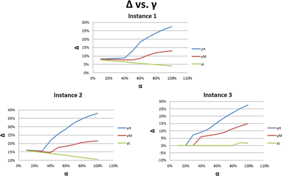
Total system profit gain in α with γ at different levels
-
Figure 4 shows an interesting pattern with respect to the bullwhip effect. For all instances, the bullwhip effect may initially increase or remain unchanged in α; it then jumps to a much higher value at some positive value of α, after which it ultimately decreases in α. We observe that the “jump” in the bullwhip effect occurs at the same point at which the increase in Δ r suddenly becomes large. We also find that the larger the value of γ, the earlier this “jump” occurs. From our numerical tests, we found that there are typically two types of promotion plan patterns for each problem instance, which we will call “Plan L” and “Plan H,” respectively. Price discounts for “Plan H” are much deeper than price discounts for “Plan L.” However, when the pass-through rate α is low, it is optimal for the supplier to adopt “Plan L” instead of “Plan H.” As the value of α increases, after reaching a certain positive value of α, the optimal promotion plan for the supplier changes from the form of “Plan L” to “Plan H,” and we call this the threshold value of α. When the value of γ is large, this means the consumers are more sensitive to retail price discounts, so, for the same level of retail discount, a higher value of γ means more new consumers, which results in a smaller threshold value of α. Because the number of new consumers attracted by “Plan H” is usually much larger than that of “Plan L,” “Plan H” typically brings a both larger system profit and a higher value of the bullwhip effect.
Fig. 4 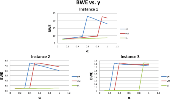
Bullwhip effect in α with γ at different levels


6 Concluding remarks
This study considered a stochastic bilevel model that simultaneously determines a supplier’s trade promotion policy and a retailer’s operations decisions. We presented a procedure which transforms the stochastic bilevel model to a deterministic single-level problem in the form of a generalized bilinear programming problem. We provided an exact solution method for solving this GBP problem, and compared this approach with Al-Khayyal’s approach and a widely-used heuristic method for solving GBPs. Based on our numerical study, our exact algorithm has proven to be quite efficient. We also provided numerical evidence that increased supplier profit and increased system profit can coexist with the bullwhip effect as a result of price promotions if: (i) the supplier accounts for the retailer’s reactions when making promotion decisions; (ii) there is a sufficient number of additional consumers who are attracted by the discounted price; and (iii) the pass-through rate is set judiciously by the retailer. In addition, this paper builds a foundation for future research. For example, we may consider the retailer’s pass-through rate as a decision variable. We are also interested in the promotion design problem when the effectiveness of a promotion depends on the supplier’s and retailer’s previous decisions. Finally, solving large-scale problem instances would likely necessitate the application of heuristic solution methods, wherein the methods we have proposed may be very useful for providing bounds on optimal solutions.
Notes
We define L P as the number of periods within the supplier’s “promotion time window,” i.e., the number of periods during which the supplier offers a discount. Because L P may equal L, the supplier may in principle offer a discount in any period. However, as noted in Blattberg and Neslin (1989), price promotions that are too frequent tend to lose their effectiveness. Thus, in practical contexts, supplier’s tend to engage in cyclical planning, wherein they tend to offer promotions periodically. As a result, we envision our model as being applied periodically, where, without loss of generality, we assume that promotions are implemented during the first L P periods of the planning horizon.
While we recognize that the pass-through rates are decision variables set by the retailer, we assume fixed values in our model for model tractability. Thus, when using this model for decision making, the supplier must parameterize on the pass-through rate in order to determine (at least approximately) the values that the retailer is likely to apply.
References
Ahuja, R. K., Magnanti, T. L., & Orlin, J. B. (1993). Network flows: theory, algorithms, and applications. New York: Prentice-Hall.
Ailawadi, K., Farris, P. W., & Shames, E. (1999). Trade promotion: essential to selling through resellers. Sloan Management Review, 41(1), 83–92.
Al-Khayyal, F. A. (1992). Generalized bilinear programming: part I. Models, applications and linear programming relaxation. European Journal of Operational Research, 60(3), 306–314.
Al-Khayyal, F. A., & Falk, J. E. (1983). Jointly constrained biconvex programming. Mathematics of Operations Research, 8(2), 273–286.
Al-Khayyal, F. A., Larsen, C., & Van Voorhis, T. (1995). A relaxation method for nonconvex quadratically constrained quadratic programs. Journal of Global Optimization, 6(3), 215–230.
Arcelus, F. J., & Srinivasan, G. (1998). Ordering policies under one time only discount and price sensitive demand. IIE Transactions, 30(11), 1057–1064.
Ardalan, A. (1991). Combined optimal price and optimal inventory replenishment policies when a sale results in increase in demand. Computers & Operations Research, 18(8), 721–730.
Ardalan, A. (1994). Optimal prices and order quantities when temporary price discounts result in increase in demand. European Journal of Operational Research, 72(1), 52–61.
Bell, D. R., & Drèze, X. (2002). Changing the channel: a better way to do trade promotions. MIT Sloan Management Review, 43(2), 42–49.
Ben-Ayed, O. (1993). Bilevel linear programming. Computers & Operations Research, 20(5), 485–501.
Berry, J. (1992). Diverting: Trade diverting is becoming ever more widespread as it grows, so does mistrust between retailer and manufacturer. Adweek’s Marketing Week, 33(20).
Besanko, D., Dubé, J. P., & Gupta, S. (2005). Own-brand and cross-brand retail pass-through. Marketing Science, 24(1), 123–137.
Blattberg, R. C., & Neslin, S. A. (1989). Sales promotion: the long and the short of it. Marketing Letters, 1(1), 81–97.
Blattberg, R. C., Eppen, G. D., & Lieberman, J. (1981). A theoretical and empirical evaluation of price deals for consumer nondurables. The Journal of Marketing, 45(1), 116–129.
Bronnenberg, B. J., Dhar, S. K., & Dubé, J. P. (2005). Market structure and the geographic distribution of brand shares in consumer package goods industries. University of Chicago Mimeograph.
Bronnenberg, B. J., Dhar, S. K., & Dubé, J. P. (2007). Consumer packaged goods in the united states: national brands, local branding. Journal of Marketing Research, 44(1), 4–13.
Cheng, F., & Sethi, S. P. (1999). A periodic review inventory model with demand influenced by promotion decisions. Management Science, 45(11), 1510–1523.
Desai, V. S. (1992). Marketing-production decisions under independent and integrated channel structure. Annals of Operations Research, 34(1), 275–306.
Drèze, X., & Bell, D. R. (2003). Creating win-win trade promotions: theory and empirical analysis of scan-back trade deals. Marketing Science, 22(1), 16–39.
Gómez, M. I., Rao, V. R., & McLaughlin, E. W. (2007). Empirical analysis of budget and allocation of trade promotions in the US supermarket industry. Journal of Marketing Research, 44(3), 410–424.
Knowledge@Wharton (2001). Pay-for-performance trade promotions can ease friction between manufacturers and retailers. http://knowledge.wharton.upenn.edu/article.cfm?articleid=409&source=rss.
Lee, H. L., Padmanabhan, V., & Whang, S. (1997). Information distortion in a supply chain: the bullwhip effect. Management Science, 43(4), 546–558.
MEI Computer Technology Group Inc. (2010). Technology Group Inc. Rebounding economy has CPG firms looking to win back customers as nearly half will spend more on trade promotions this year. http://www.prnewswire.com/news-releases/rebounding-economy-has-cpg-firms-looking-to-win-back-customers-as-nearly-half-will-spend-more-on-trade-promotions-this-year-96877409.html.
Miller, R. (1997). Does everyone have a price. Marketing, 30(3).
Murry, J. P. Jr., & Heide, J. B. (1998). Managing promotion program participation within manufacturer-retailer relationships. The Journal of Marketing, 62(1), 58–68.
Muu, L. D., & Quy, N. V. (2003). A global optimization method for solving convex quadratic bilevel programming problems. Journal of Global Optimization, 26(2), 199–219.
MWPVL International Inc. (2010). The grocery distribution center network in North America. http://www.mwpvl.com/html/grocery_distribution_network.html.
Neslin, S. A., Powell, S. G., & Stone, L. S. (1995). The effects of retailer and consumer response on optimal manufacturer advertising and trade promotion strategies. Management Science, 41(5), 749–766.
Petrik, M., & Zilberstein, S. (2011). Robust approximate bilinear programming for value function approximation. Journal of Machine Learning Research, 12, 3027–3063.
Petruzzi, N. C., & Dada, M. (1999). Pricing and the newsvendor problem: a review with extensions. Operations Research, 47(2), 183–194.
Sherali, H. D., & Alameddine, A. (1992). A new reformulation-linearization technique for bilinear programming problems. Journal of Global Optimization, 2(4), 379–410.
Sherali, H. D., & Shetty, C. M. (1980). A finitely convergent algorithm for bilinear programming problems using polar cuts and disjunctive face cuts. Mathematical Programming, 19(1), 14–31.
Sogomonian, A. G., & Tang, C. S. (1993). A modeling framework for coordinating promotion and production decisions within a firm. Management Science, 39(2), 191–203.
Su, Y., & Geunes, J. (2012). Price promotions, operations cost, and profit in a two-stage supply chain. Omega.
Thowsen, G. T. (1975). A dynamic, nonstationary inventory problem for a price/quantity setting firm. Naval Research Logistics Quarterly, 22(3), 461–476.
Upasani, A., & Uzsoy, R. (2008). Incorporating manufacturing lead times in joint production-marketing models: a review and some future directions. Annals of Operations Research, 161(1), 171–188.
Vicente, L. N., Calamai, P. H., & Júdice, J. J. (1992). Generation of disjointly constrained bilinear programming test problems. Computational Optimization and Applications, 1(3), 299–306.
Wen, U. P., & Hsu, S. T. (1991). Linear bi-level programming problems–a review. Journal of the Operational Research Society, 42(2), 125–133.
Xiao, T., Yu, G., Sheng, Z., & Xia, Y. (2005). Coordination of a supply chain with one-manufacturer and two-retailers under demand promotion and disruption management decisions. Annals of Operations Research, 135(1), 87–109.
Author information
Authors and Affiliations
Corresponding author
Appendix
Appendix
1.1 A.1 Decomposition of uncapacitated minimum cost flow problem
This section provides a proof that an uncapacitated minimum cost flow problem can be decomposed into a set of shortest path problems.
Theorem 1
A single-origin, N-destination uncapacitated minimum cost flow problem can be decomposed into N shortest path problems that do not depend on the demand level.
Proof
Assume without loss generality that we have a directed network G=(V,E), where V={0,1,…,N} is the set of nodes and E is the set of arcs. Each arc (i,j)∈E has an associated cost c ij that denotes the cost per unit flow on that arc. We also assume that each arc has an infinite capacity, i.e., there is no upper bound on the maximum amount that can flow on any arc. The network has a unique node 0, called the source, with supply \(\sum_{i=1}^{N} d_{i}\). For each nonsource node i∈V, we associate with it a demand level d i (≥0). The single-origin N-destination uncapacitated minimum cost flow problem is to determine a minimum cost flow through the uncapacitated network in order to satisfy demands at the N nonsource nodes from available supplies at the source node 0. The decision variables in this problem are arc flows, and we represent the flow on an arc (i,j)∈E by x ij . The single-origin N-destination uncapacitated minimum cost flow problem can be formulated as follows:
The flow decomposition theorem (Ahuja et al. 1993) implies that the flow x ij on each arc (i,j)∈E can be decomposed by destination, with \(x_{ij}^{l}\) representing of flow on arc (i,j) used to satisfy demand at node l. With this notation, we can reformulate the single-origin N-destination uncapacitated minimum cost flow problem as follows:
By definition, we have \(x_{ij} = \sum_{l=1}^{L} x_{ij}^{l}\). Suppose we define variables \(y_{ij}^{l}=\frac{x_{ij}^{l}}{d_{l}}\). Using these, the single-origin N-destination uncapacitated minimum cost flow problem can be expressed as follows:
In this above formulation, the set of feasible solutions Y can be decomposed into N sets Y 1,Y 2,…,Y N, where
By observation, the variables for each subset do not appear in any other set. Consequently, we can decompose UMCP″ into N shortest path problems which do not depend on the demand level in the following formulation:
After solving all of these N shortest path problems, we can obtain the solutions to the original UMCP using the following relationship:
□
1.2 A.2 Detailed Al-Khayyal approach
The detailed Al-Khayyal branch-and-bound algorithm is shown in Algorithm 2. After initializing the branch-and-bound tree in line 1, the algorithm repeats the Main Step in the while loop in lines 2–29 until the optimality gap is less than a predetermined value ϵ. At the start of each iteration k of the while loop, a node (u,v) is selected and removed from tree T k in line 3. In lines 4 and 5, the linear program LP(Ω (u,v)) is solved to obtain the solution \(\bar{\varLambda}\) and the corresponding optimal value \(\varPhi (\bar{\varLambda})\) is assigned to UB k . In lines 6–16, the current iteration lower bound LB k is obtained and the partitioning index (p,q) is found by checking the optimality and the feasibility of the solution \(\bar{\varLambda}\). After finding (p,q), partition the region Ω (u,v) into two mutually exclusive and exhaustive subregions in lines 18–21. At the end of the while loop, the branch-and-bound tree is updated by three types of operations in lines 22–27. Included here are
-
1.
update the lower bound of the problem if LB<LB k as follows:
$$\mathit{LB} \gets \mathit{LB}_k \text{ and } \bigl(x^*,y^*,z^*,\pi^*\bigr) \gets ( \bar{x},\bar{y},\bar{z},\bar{\pi}); $$ -
2.
update the node set at iteration k as
$$T_k \gets T_k -\bigl\{ (m,n)\in T_k: \mathit{UB}^{(m,n)} \leq \mathit{LB}\bigr\} ; $$ -
3.
update the upper bound of the problem as
$$\mathit{UB} =\max \bigl\{ \mathit{UB}^{(m,n)}, \forall (m,n) \in T_{k+1}\bigr\} . $$

Al-Khayyal’s Branch-and-Bound algorithm
Rights and permissions
About this article
Cite this article
Su, Y., Geunes, J. Multi-period price promotions in a single-supplier, multi-retailer supply chain under asymmetric demand information. Ann Oper Res 211, 447–472 (2013). https://doi.org/10.1007/s10479-013-1485-2
Published:
Issue Date:
DOI: https://doi.org/10.1007/s10479-013-1485-2