Conditional gradient algorithms for norm-regularized smooth convex optimization

Abstract

Motivated by some applications in signal processing and machine learning, we consider two convex optimization problems where, given a cone $K$, a norm $\Vert \cdot \Vert$ and a smooth convex function $f$, we want either (1) to minimize the norm over the intersection of the cone and a level set of $f$, or (2) to minimize over the cone the sum of $f$ and a multiple of the norm. We focus on the case where (a) the dimension of the problem is too large to allow for interior point algorithms, (b) $\Vert \cdot \Vert$ is “too complicated” to allow for computationally cheap Bregman projections required in the first-order proximal gradient algorithms. On the other hand, we assume that it is relatively easy to minimize linear forms over the intersection of $K$ and the unit $\Vert \cdot \Vert$-ball. Motivating examples are given by the nuclear norm with $K$ being the entire space of matrices, or the positive semidefinite cone in the space of symmetric matrices, and the Total Variation norm on the space of 2D images. We discuss versions of the Conditional Gradient algorithm capable to handle our problems of interest, provide the related theoretical efficiency estimates and outline some applications.

1 Introduction

We consider two norm-regularized convex optimization problems as follows:

$$\begin{aligned}&\displaystyle \hbox {[norm minimization]}\min _{x\in K}\,\Vert x\Vert ,\;\;\hbox {subject to}\;\;f(x)\le 0,\end{aligned}$$

(1)

$$\begin{aligned}&\displaystyle \hbox {[penalized minimization]}\min _{x \in K } \, f(x) + \kappa \Vert x \Vert \end{aligned}$$

(2)

where $f$ is a convex function with Lipschitz continuous gradient, $K$ is a closed convex cone in a Euclidean space $E, \Vert \cdot \Vert$ is some norm, and $\kappa$ is a positive parameter. Problems such as (1) and (2) are of definite interest for signal processing and machine learning. In these applications, $f(x)$ quantifies the discrepancy between the observed noisy output of some parametric model and the output of the model with candidate vector $x$ of parameters. Most notably, $f$ is the quadratic penalty: $f(x)=\frac{1}{2}\Vert \mathcal{A}x - y\Vert _2^2-\delta$, where $\mathcal{A}x$ is the predicted output of the linear regression model $x\mapsto \mathcal{A}x$, and $y=\mathcal{A}x_*+\xi$, where $x_*$ is the vector of true parameters, $\xi$ is the observation error, and $\delta$ is an a priori upper bound on ${1\over 2}\Vert \xi \Vert _2^2$. The cone $K$ sums up a priori information on the parameter vectors (e.g., $K=E$—no a priori information at all, or $E={\mathbf {R}}^p, K={\mathbf {R}}^p_+$, or $E={\mathbf {S}}^p$, the space of symmetric $p\times p$ matrices, and $K={\mathbf {S}}^p_+$, the cone of positive semidefinite matrices, as is the case of covariance matrices recovery). Finally, $\Vert \cdot \Vert$ is a regularizing norm “promoting” a desired property of the recovery, e.g., the sparsity-promoting norm $\ell _1$ on $E={\mathbf {R}}^n$, or the low rank promoting nuclear norm on $E={\mathbf {R}}^{p\times q}$, or the Total Variation (TV) norm, as in image reconstruction.

In the large-scale case, first-order algorithms of proximal-gradient type are popular to tackle such problems, see [34] for a recent overview. Among them, the celebrated Nesterov optimal gradient methods for smooth and composite minimization [26–28], and their stochastic approximation counterparts [21], are now state-of-the-art in compressive sensing and machine learning. These algorithms enjoy the best known so far theoretical estimates (and in some cases, these estimates are the best possible for the first-order algorithms). For instance, Nesterov’s algorithm for penalized minimization [27, 28] solves (2) to accuracy $\epsilon$ in $O(D_0\sqrt{L/\epsilon })$ iterations, where $L$ is the properly defined Lipschitz constant of the gradient of $f$, and $D_0$ is the initial distance to the optimal set, measured in the norm $\Vert \cdot \Vert$. However, applicability and efficiency of proximal-gradient algorithms in the large-scale case require from the problem to possess “favorable geometry” (for details, see [28, Section A.6]). To be more specific, consider proximal-gradient algorithm for convex minimization problems of the form

$$\begin{aligned} \min _{x} \; \{f(x):\;\Vert x\Vert \le 1, \,x\in K\}. \end{aligned}$$

(3)

The comments to follow, with slight modifications, are applicable to problems such as (1) and (2) as well. In this case, a proximal-gradient algorithm operates with a “distance generating function” (d.g.f.) defined on the domain of the problem and 1-strongly convex w.r.t. the norm $\Vert \cdot \Vert$. Each step of the algorithm requires minimizing the sum of the d.g.f. and a linear form. The efficiency estimate of the algorithm depends on the variation of the d.g.f. on the domain and on regularity of $f$ w.r.t. $\Vert \cdot \Vert$.¹ As a result, in order for a proximal-gradient algorithm to be practical in the large scale case, two “favorable geometry” conditions should be met: (a) the outlined sub-problems should be easy to solve, and (b) the variation of the d.g.f. on the domain of the problem should grow slowly (if at all) with problem’s dimension. Both these conditions indeed are met in many applications; see, e.g., [2, 20] for examples. This explains the recent popularity of this family of algorithms.

However, sometimes conditions (a) and/or (b) are violated, and application of proximal algorithms becomes questionable. For example, for the case of $K=E$, (b) is violated for the usual $\Vert \cdot \Vert _\infty$-norm on ${\mathbf {R}}^p$ or, more generally, for $\Vert \cdot \Vert _{2\rightarrow \infty }$ norm on the space of $p\times q$ matrices given by

$$\begin{aligned} \Vert x\Vert _{2\rightarrow \infty }{:=}\max \limits _{u\in {\mathbf {R}}^q:\Vert u\Vert _2\le 1}\Vert xu\Vert _\infty =\max _{1\le j\le p} \Vert \hbox {Row}_j(x)\Vert _2, \end{aligned}$$

where $\hbox {Row}_j^T(x)$ denotes the $j$th row of $x$. Here the variation of (any) d.g.f. on problem’s domain is at least $p$. As a result, in the case in question the theoretical iteration complexity of a proximal algorithm grows rapidly with the dimension $p$. Furthermore, for some high-dimensional problems which do satisfy (b), solving the sub-problem can be computationally challenging. Examples of such problems include nuclear-norm-based matrix completion, Total Variation-based image reconstruction, and multi-task learning with a large number of tasks and features. This corresponds to $\Vert \cdot \Vert$ in (1) or (2) being the nuclear norm [11, 14] or the TV-norm.

These limitations recently motivated alternative approaches, which do not rely upon favorable geometry of the problem domain and/or do not require to solve hard sub-problems at each iteration, and triggered a renewed interest in the Conditional Gradient (CndG) algorithm. This algorithm, also known as the Frank–Wolfe algorithm, which is historically the first method for smooth constrained convex optimization, originates from [9], and was extensively studied in the 70-s (see, e.g., [6, 8, 29] and references therein). CndG algorithms work by minimizing a linear form on the problem domain at each iteration; this auxiliary problem clearly is easier, and in many cases—significantly easier than the auxiliary problem arising in proximal-gradient algorithms. Conditional gradient algorithms for collaborative filtering were studied recently [17, 18], some variants and extensions were studied in [7, 11, 33]. Those works consider constrained formulations of machine learning or signal processing problems, i.e., minimizing the discrepancy $f(x)$ under a constraint on the norm of the solution, as in (3). On the other hand, CndG algorithms for other learning formulations, such as norm minimization (1) or penalized minimization (2) remain open issues. An exception is the work of [7, 11], where a Conditional Gradient algorithm for penalized minimization was studied, although the efficiency estimates obtained in that paper were suboptimal. In this paper (for its conference version, see [12]) we present CndG-type algorithms aimed at solving norm minimization and penalized minimization problems² and provide theoretical efficiency guarantees for these algorithms.

The main body of the paper is organized as follows. In Sect. 2, we present detailed setting of problems (1), (2) along with basic assumptions on the “computational environment” required by the CndG-based algorithms we are developing. These algorithms and their efficiency bounds are presented in Sect. 3 (problem (1)) and 5 (problem (2). In Sect.  6 we outline some applications, and in Sect. 7 present preliminary numerical results. All proofs are relegated to the “Appendix”.

2 Problem statement

Throughout the paper, we shall assume that $K\subset E$ is a closed convex cone in Euclidean space $E$; we loose nothing by assuming that $K$ linearly spans $E$. We assume, further, that $\Vert \cdot \Vert$ is a norm on $E$, and $f:K\rightarrow {\mathbf {R}}$ is a convex function with Lipschitz continuous gradient, so that

$$\begin{aligned} \Vert f'(x)-f'(y)\Vert _*\le L_f \Vert x-y\Vert \,\,\forall x,y\in K, \end{aligned}$$

where $\Vert \cdot \Vert _*$ denotes the norm dual to $\Vert \cdot \Vert$ ³

$$\begin{aligned} \forall x,y\in K: f(y)\le f(x)+\langle f'(x),y-x\rangle +{L_f\over 2}\Vert y-x\Vert ^2. \end{aligned}$$

(4)

We consider two kinds of problems, detailed below.

Norm-minimization. Such problems correspond to

$$\begin{aligned} \rho _*=\min _{x} \left\{ \Vert x\Vert :\,x\in K,\,f(x)\le 0\right\} . \end{aligned}$$

(5)

To tackle (5), we consider the following parametric family of problems

$$\begin{aligned} {\mathop {\hbox {Opt}}}(\rho )=\min \{f(x):\;\Vert x\Vert \le \rho , \,x\in K\} \, . \end{aligned}$$

(6)

Note that whenever (5) is feasible, which we assume from now on, we have

$$\begin{aligned} \rho _*=\min \{\rho \ge 0:\; {\mathop {\hbox {Opt}}}(\rho )\le 0\}, \end{aligned}$$

(7)

and both problems (5), (7) can be solved.

Given a tolerance $\epsilon >0$, we want to find an $\epsilon$-solution to the problem, that is, $x_\epsilon \in K$ such that

$$\begin{aligned} \Vert x_\epsilon \Vert \le \rho _*\;\hbox {and}\;f(x_\epsilon )\le \epsilon . \end{aligned}$$

(8)

Getting back to the problem of interest (5), $x_\epsilon$ is then “super-optimal” and $\epsilon$-feasible.

Penalized norm minimization. These problems write as

$$\begin{aligned} {\mathop {\hbox {Opt}}}=\min _{x} \left\{ f(x)+\kappa \Vert x\Vert :\;x\in K\right\} \, . \end{aligned}$$

(9)

A equivalent formulation is

$$\begin{aligned} {\mathop {\hbox {Opt}}}=\min _{x,r} \left\{ F([x;r])=\kappa r+f(x):x\in K,\Vert x\Vert \le r\right\} . \end{aligned}$$

(10)

We shall refer to (10) as the problem of composite optimization (CO). Given a tolerance $\epsilon >0$, our goal is to find an $\epsilon$-solution to (10), defined as a feasible solution $(x_\epsilon , r_\epsilon )$ to the problem satisfying $F([x_\epsilon ;r_\epsilon ])-{\mathop {\hbox {Opt}}}\le \epsilon$. Note that in this case $x_\epsilon$ is an $\epsilon$-solution, in the similar sense, to (9).

Special case. In many applications where problems (5) and (9) arise, the function $f$ enjoys a special structure:

$$\begin{aligned} f(x) = \phi (\mathcal{A}x-b), \end{aligned}$$

where $x\mapsto \mathcal{A}x-b$ is an affine mapping from $E$ to ${\mathbf {R}}^m$, and $\phi (\cdot ):{\mathbf {R}}^m\rightarrow {\mathbf {R}}$ is a convex function with Lipschitz continuous gradient; we shall refer to this situation as to special case. In such case, the quantity $L_f$ can be bounded as follows. Let $\pi (\cdot )$ be some norm on ${\mathbf {R}}^m, \pi _*(\cdot )$ be the conjugate norm, and $\Vert \mathcal{A}\Vert _{\Vert \cdot \Vert ,\pi }$ be the norm of the linear mapping $x\mapsto \mathcal{A}x$ induced by the norms $\Vert \cdot \Vert , \pi (\cdot )$ on the argument and the image spaces:

$$\begin{aligned} \Vert \mathcal{A}\Vert _{\Vert \cdot \Vert ,\pi (\cdot )}=\max _{x\in E}\{\pi (\mathcal{A}x):\Vert x\Vert \le 1\}. \end{aligned}$$

Let also $L_{\pi (\cdot )}[\phi ]$ be the Lipschitz constant of the gradient of $\phi$ induced by the norm $\pi (\cdot )$, so that

$$\begin{aligned} \pi _*(\phi '(y)-\phi '(y')) \le L_{\pi (\cdot )}[\phi ]\pi (y-y')\,\,\forall y,y'\in {\mathbf {R}}^m. \end{aligned}$$

Then, one can take as $L_f$ the quantity

$$\begin{aligned} L_f=L_{\pi (\cdot )}[\phi ] \Vert \mathcal{A}\Vert _{\Vert \cdot \Vert ,\pi (\cdot )}^2. \end{aligned}$$

(11)

Example 1

Quadratic fit. In many applications, we are interested in $\Vert \cdot \Vert _2$-discrepancy between $\mathcal{A}x$ and $b$; the related choice of $\phi (\cdot )$ is $\phi (y)={1\over 2}y^Ty$. Specifying $\pi (\cdot )$ as $\Vert \cdot \Vert _2$, we get $L_{\Vert \cdot \Vert _2}[\phi ]=1$.

Example 2

Smoothed $\ell _\infty$ fit. When interested in $\Vert \cdot \Vert _\infty$ discrepancy between $\mathcal{A}x$ and $b$, we can use as $\phi$ the function $\phi (y)={1\over 2} \Vert y\Vert _\beta ^2$, where $\beta \in [2,\infty )$. Taking $\pi (\cdot )$ as $\Vert \cdot \Vert _\infty$, we get

$$\begin{aligned} L_{\Vert \cdot \Vert _\infty }[\phi ]\le (\beta -1)m^{2/\beta }. \end{aligned}$$

Note that

$$\begin{aligned} {1\over 2}\Vert y\Vert _\infty ^2\le \phi (y)\le {m^{2/\beta }\over 2} \Vert y\Vert _\infty ^2, \end{aligned}$$

so that for $\beta =O(1)\ln (m)$ and $m$ large enough (specifically, such that $\beta \ge 2$), $\phi (y)$ is within absolute constant factor of ${1\over 2}\Vert y\Vert _\infty ^2$. The latter situation can be interpreted as $\phi$ behaving as ${1\over 2}\Vert \cdot \Vert _\infty ^2$. At the same time, with $\beta =O(1)\ln (m), L_{\Vert \cdot \Vert _\infty }[\phi ]\le O(1)\ln (m)$ grows with $m$ logarithmically.

Another widely used choice of $\phi (\cdot )$ for this type of discrepancy is “logistic” function

$$\begin{aligned} \phi (y)={1\over \beta }\ln \left( \sum _{i=1}^m \left[ e^{\beta y_i}+e^{-\beta y_i}\right] \right) . \end{aligned}$$

For $\pi (\cdot )=\Vert \cdot \Vert _{\infty }$ we easily compute $L_{\Vert \cdot \Vert _\infty }[\phi ]\le \beta$ and $\Vert y\Vert _\infty \le \phi (y)\le \Vert y\Vert _\infty + \ln (2m)/\beta$.

Note that in some applications we are interested in “one-sided” discrepancies quantifying the magnitude of the vector $[\mathcal{A}x - b]_+=[\max [0,(\mathcal{A}x-b)_1];\ldots ;\max [0,(\mathcal{A}x -b)_m]]$ rather than the the magnitude of the vector $\mathcal{A}x -b$ itself. Here, instead of using $\phi (y)={\small \frac{1}{2}}\Vert y\Vert ^2_\beta$ in the context of examples 1 and 2, one can use the functions $\phi _+(y)=\phi ([y]_+)$. In this case the bounds on $L_{\pi (\cdot )}[\phi _+]$ are exactly the same as the above bounds on $L_{\pi (\cdot )}[\phi ]$. The obvious substitute for the two-sided logistic function is its “one-sided version:” $\phi _+(y)={1\over \beta }\ln \left( \sum _{i=1}^m \left[ e^{\beta y_i}+1\right] \right)$ which obeys the same bound for $L_{\pi (\cdot )}[\phi _+]$ as its two-sided analogue.

First-order and linear optimization oracles. We assume that $f$ is represented by a first-order oracle—a routine which, given on input a point $x\in K$, returns the value $f(x)$ and the gradient $f'(x)$ of $f$ at $x$. As about $K$ and $\Vert \cdot \Vert$, we assume that they are given by a Linear Optimization (LO) oracle which, given on input a linear form $\langle \eta ,\cdot \rangle$ on $E$, returns a minimizer $x[\eta ]$ of this linear form on the set $\{x\in K:\Vert x\Vert \le 1\}$. We assume w.l.o.g. that for every $\eta , x[\eta ]$ is either zero, or is a vector of the $\Vert \cdot \Vert$-norm equal to 1. To ensure this property, it suffices to compute $\langle \eta ,x[\eta ]\rangle$ for $x[\eta ]$ given by the oracle; if this inner product is 0, we can reset $x[\eta ]=0$, otherwise $\Vert x[\eta ]\Vert$ is automatically equal to 1.

Note that an LO oracle for $K$ and $\Vert \cdot \Vert$ allows to find a minimizer of a linear form of $z=[x;r]\in E^+{:=}E\times {\mathbf {R}}$ on a set of the form $K^+[\rho ]=\{[x;r]\in E^+: x\in K, \Vert x\Vert \le r\le \rho \}$ due to the following observation:

Lemma 1

Let $\rho \ge 0$ and $\eta ^+=[\eta ;\sigma ]\in E^+$. Consider the linear form $\ell (z)=\langle \eta ^+,z\rangle$ of $z=[x;r]\in E^+$, and let

$$\begin{aligned} z^+=\left\{ \begin{array}{l@{\quad }l}\rho [x[\eta ];1],&{}\langle \eta ^+,[x[\eta ];1]\rangle \le 0,\\ 0,&{}\hbox {otherwise}\\ \end{array}\right. \!. \end{aligned}$$

Then $z^+$ is a minimizer of $\ell (z)$ over $z\in K^+[\rho ]$, When $\sigma =0$, one has $z^+=\rho [x[\eta ];1]$.

Indeed, by the definition of $x[\eta ]$, for all $z=[x;r]\in K^+[\rho ]$ we have $\ell (r[x[\eta ];1])\le \ell (z)$. Now, let $z_*=[x_*;r_*]$ be a minimizer of $\ell (\cdot )$ over $K^+[\rho ]$, then $\ell (z^*)\le \ell (z_*)$, where $z^*{:=}r_*[x[\eta ];1]\in K^+[\rho ]$. We conclude that any minimizer of $\ell (\cdot )$ over the segment $\{s[x[\eta ];1]:0\le s\le \rho \}$ is also a minimizer of $\ell (\cdot )$ over $K^+[\rho ]$. It remains to note that the vector $z^+$ in the lemma premise clearly is a minimizer of $\ell (\cdot )$ on the above segment.

3 Conditional gradient algorithm

In this section, we present an overview of the properties of the standard Conditional Gradient algorithm, and highlight some memory-based extensions. These properties are not new. However, since they are key for the design of our proposed algorithms in the next sections, we present them for further reference.

3.1 Conditional gradient algorithm

Let $E$ be a Euclidean space and $X$ be a closed and bounded convex set in $E$ which linearly spans $E$. Assume that $X$ is given by a LO oracle—a routine which, given on input $\eta \in E$, returns an optimal solution $x_X[\eta ]$ to the optimization problem

$$\begin{aligned} \min _{x\in X} \, \langle \eta ,x\rangle \end{aligned}$$

(cf. Sect.  2). Let $f$ be a convex differentiable function on $X$ with Lipschitz continuous gradient $f'(x)$, so that

$$\begin{aligned} \forall x,y\in X: f(y)\le f(x)+\langle f'(x),y-x\rangle +{{\small \frac{1}{2}}}L\Vert y-x\Vert _X^2, \end{aligned}$$

(12)

where $\Vert \cdot \Vert _X$ is the norm on $E$ with the unit ball $X-X$.⁴ We intend to solve the problem

$$\begin{aligned} f_*=\min _{x\in X} f(x). \end{aligned}$$

(13)

A generic CndG algorithm is a recurrence which builds iterates $x_t \in X, t=1,2,\ldots$, in such a way that

$$\begin{aligned} f(x_{t+1})\le f(\widetilde{x}_{t+1}), \end{aligned}$$

(14)

where

$$\begin{aligned} \begin{array}{rcl} \widetilde{x}_{t+1}&{}=&{}x_t+\gamma _t[x_t^+-x_t],\;\;\hbox { with } x_t^+=x_X[f'(x_t)] \quad \hbox {and}\quad \gamma _t={2\over t+1}.\\ \end{array} \end{aligned}$$

(15)

As a byproduct of running generic CndG, after $t$ steps we have at our disposal the quantities

$$\begin{aligned} f_{*,\tau }&= \min \limits _{x\in X}\left[ f(x_\tau )+\langle f'(x_\tau ),x-x_\tau \rangle \right] \nonumber \\&= f(x_\tau )-\langle f'(x_\tau ),x_\tau -x_X[f'(x_\tau )]\rangle ,\,\,1\le \tau \le t, \end{aligned}$$

(16)

which, by convexity of $f$, are lower bounds on $f_*$. Consequently, at the end of step $t$ we have at our disposal a lower bound

$$\begin{aligned} f_*^t{:=}\max _{1\le \tau \le t} f_{*,\tau }\le f_*,\,t=1,2,\ldots \end{aligned}$$

(17)

on $f_*$.

Finally, we define the approximate solution $\bar{x}_t$ found in course of $t=1,2,\ldots$ steps as the best—with the smallest value of $f$—of the points $x_1,\ldots ,x_t$. Note that $\bar{x}_t\in X$.

The following statement summarizes the well known properties of CndG [6, 8, 17, 29] (to make the presentation self-contained, we provide in “Appendix” the proof).

Theorem 1

For a generic CndG algorithm we have

$$\begin{aligned} f(\bar{x}_t)-f_*\le f(\bar{x}_t)-f^t_*\le f(x_t)-f^t_*\le {2L\over t+1},\quad t\ge 2. \end{aligned}$$

(18)

Some remarks regarding the conditional algorithm are in order.

Certifying quality of approximate solutions. An attractive property of CndG is the presence of online lower bound $f_*^t$ on $f_*$ which certifies the theoretical rate of convergence of the algorithm. This accuracy certificate, first established in a different form in [6], see also [17], also provides a valuable stopping criterion when running the algorithm in practice.

CndG algorithm with memory. When computing the next search point $x_{t+1}$, the simplest CndG algorithm defined by the recursion $x_{t+1}= x_{t}+{2\over 2+1}[x_t^+-x_t]$ only uses the latest answer $x_t^+=x_X[f'(x_t)]$ of the LO oracle. Meanwhile, the CndGalgorithm can be modified to make use of information supplied by previous oracle calls; we refer to this modification as CndG with memory (CndGM).⁵ Assume that we have already carried out $t-1$ steps of the algorithm and have at our disposal current iterate $x_t\in X$ (with $x_1$ selected as an arbitrary point of $X$) along with previous iterates $x_\tau , \tau <t$ and the vectors $f'(x_\tau ), x_\tau ^+=x_X[f'(x_\tau )]$. At the step, we compute $f'(x_t)$ and $x^+_t=x_X[f'(x_t)]$. Thus, at this point in time we have at our disposal $2t$ points $x_\tau ,x^+_\tau , 1\le \tau \le t$, which belong to $X$. Let $X_t$ be subset of these points, with the only restriction that the points $x_t, x^+_t$ are selected, and let us define the next iterate $x_{t+1}$ as

$$\begin{aligned} x_{t+1}\in \mathop {\mathrm{Argmin}}\limits _{x\in \mathrm{Conv}(X_t)} f(x), \end{aligned}$$

(19)

that is,

$$\begin{aligned} x_{t+1}=\sum _{x\in X_t}\lambda ^t_x x,\,\,\lambda ^t\in \mathop {\mathrm{Argmin}}\limits _{\lambda ^t=\{\lambda _x\}_{x\in X_t}} \left\{ f\left( \sum _{x\in X_t} \lambda _x x\right) :\;\lambda \ge 0,\;\sum _{x\in X_t}\lambda _x=1\right\} . \end{aligned}$$

(20)

Clearly, it is again a generic CndG algorithm, so that conclusions in Theorem 1 are fully applicable to CndGM. Note that the “classical” CndG algorithm per se is nothing but CndGM with $X_t=\{x_t,x_t^+\}$ and $M=2$ for all $t$.

In the above description of CndGM we assumed that the set $X_t$ is a subset of points $x_\tau , x^+_\tau , 1\le \tau \le t$, containing $x_t$ and $x_t^+$. Note that we can try to improve the accuracy of the algorithm by adding to $X_t$, along with $x_t, x_t^+$, some other points of $X$. Recall, that after $t$ iterations of the method we have at our disposal, along with $t$ iterates $x_\tau \in X$, the corresponding values $f(x_\tau )$ and gradients $f'(x_\tau ),\;1\le \tau \le t$. Let $X^b_t$ be a subset of $\{x_1,\ldots ,x_t\}$ of cardinality $m$, and let us define $x^b_t$ as a minimizer

$$\begin{aligned} x^b_t\in \mathop {\mathrm{Argmin}}_{u\in X} \left\{ f^b_t(u){:=}\max _{x\in X^b_t} [f(x)+\langle f'(x),u-x\rangle ]\right\} , \end{aligned}$$

of the current “bundle approximation” $f^b_t$ of $f$; note that the quantity $f^b_t(x^b_t)$ bounds from below the optimal value $f_*$ of (13). One can include the point $x^b_t$ into $X_t$ and replace the current lower bound $f_*^t$ on $f_*$ with $\max \{f_*^t,f^b_t(x^b_t)\}$.⁶

It remains to notice that if the cardinality $m$ of the “bundle” is small the price of computing $x^b_t$ is comparable to that of $x_t^+$. Indeed, when denoting $x_{\tau _1},\,\ldots ,\,x_{\tau _m}$ the elements of $X^b_t$ and $\Lambda =\{\lambda \in {\mathbf {R}}^m:\;\lambda _i\ge 0, \,\sum _{i=1}^m\lambda _i=1\}$, one has

$$\begin{aligned} \min _{u\in X} f^b_t(u)&= \min _{u\in X} \left\{ \max _{\lambda \in \Lambda } \sum _{i=1}^m \lambda _i [f(x_{\tau _i})+\langle f'(x_{\tau _i}),u-x_{\tau _i}\rangle ]\right\} \\&= \max _{\lambda \in \Lambda }\left\{ F(\lambda ){:=}\min _{u\in X}\sum _{i=1}^m \lambda _i[f(x_{\tau _i})+\langle f'(x_{\tau _i}),u-x_{\tau _i}\rangle ]\right\} . \end{aligned}$$

When $m$ is small, one can find high accuracy approximate solutions $\widehat{\lambda }$ to the problem of maximizing $F$ over the standard simplex using (linearly converging) cutting plane algorithms, for which LO oracle will readily supply first order information. Then corresponding “primal” approximate solutions $\widehat{x}^b_t$ can be recovered using dual certificates, as described in [5, 24].

CndGM: implementation issues. Assume that the cardinalities of the sets $X_t$ in CndGM are bounded by some $M \ge 2$. In this case, implementation of the method requires solving at every step an auxiliary problem (20) of minimizing over the standard simplex of dimension $\le M-1$ a smooth convex function given by a first-order oracle induced by the first-oracle for $f$. When $M$ is a once for ever fixed small integer, the arithmetic cost of solving this problem within machine accuracy by, say, the Ellipsoid algorithm is dominated by the arithmetic cost of just $O(1)$ calls to the first-order oracle for $f$. Thus, CndGM with small $M$ can be considered as implementable.⁷

Note that in the special case (Sect.  2), where $f(x)=\phi (Ax-b)$, assuming $\phi (\cdot )$ and $\phi '(\cdot )$ easy to compute, as is the case in most of the applications, the first-order oracle for the auxiliary problems arising in CndGM becomes cheap (cf. [39]). Indeed, in this case (20) reads

$$\begin{aligned} \min _{\lambda ^t}\left\{ g_t(\lambda ^t):=\phi \left( \sum \limits _{x\in X_t}\lambda ^t_xAx-b\right) : \begin{array}{l} \lambda ^t=\{\lambda ^t_x\}_{x\in X_t}\ge 0,\\ \mathop {\sum }\limits _{x\in X_t}\lambda ^t_x=1\\ \end{array}\right\} . \end{aligned}$$

(22)

It follows that all we need to get a computationally cheap access to the first-order information on $g_t(\lambda ^t)$ for all values of $\lambda ^t$ is to have at our disposal the matrix-vector products $Ax, x\in X_t$. With our construction of $X_t$, the only two “new” elements in $X_t$ (those which were not available at preceding iterations) are $x_t$ and $x^+_t$, so that the only two new matrix-vector products we need to compute at iteration $t$ are $Ax_t$ (which usually is a byproduct of computing $f'(x_t)$) and $Ax_t^+$. Thus, we can say that the “computational overhead,” as compared to computing $f'(x_t)$ and $x_t^+=x_X[f'(x_t)]$, needed to get easy access to the first-order information on $g_t(\cdot )$ reduces to computing the single matrix-vector product $Ax_t^+$.

4 Conditional gradient algorithm for parametric optimization

In this section, we describe a multi-stage algorithm to solve the parametric optimization problem (6), (7), using the conditional algorithm to solve inner sub-problems (6), (7). The idea, originating from [22] (see also [19, 26, 28]), is to use a Newton-type method for approximating from below the positive root $\rho _*$ of ${\mathop {\hbox {Opt}}}(\rho )$, with (inexact) first-order information on ${\mathop {\hbox {Opt}}}(\cdot )$ yielded by approximate solving the optimization problems defining ${\mathop {\hbox {Opt}}}(\cdot )$; the difference with the outlined references is that now we solve these problems with the CndG algorithm.

Our algorithm works stagewise. At the beginning of stage $s=1,2,\ldots$, we have at hand a lower bound $\rho _s$ on $\rho _*$, with $\rho _1$ defined as follows:

We compute $f(0), f'(0)$ and $x[f'(0)]$. If $f(0)\le \epsilon$ or $x[f'(0)]=0$, we are done—the pair ($\rho =0, x=0$) is an $\epsilon$-solution to (7) in the first case, and is an optimal solution to the problem in the second case (since in the latter case $0$ is a minimizer of $f$ on $K$, and (7) is feasible). Assume from now on that the above options do not take place (“nontrivial case”), and let

$$\begin{aligned} d=-\langle f'(0),x[f'(0)]\rangle . \end{aligned}$$

Due to the origin of $x[\cdot ], d$ is positive, and $f(x)\ge f(0)+\langle f'(0),x\rangle \ge f(0)-d\Vert x\Vert$ for all $x\in K$, which implies that $\rho _*\ge \rho _1{:=}{f(0)\over d}>0.$

At stage $s$ we apply a generic CndG algorithm to the auxiliary problem

$$\begin{aligned} {\mathop {\hbox {Opt}}}(\rho _s)=\min _x\{f(x):\,x\in K[\rho _s]\},\quad K[\rho ]=\{x\in K:\Vert x\Vert \le \rho \}, \end{aligned}$$

(23)

Note that the LO oracle for $K, \Vert \cdot \Vert$ induces an LO oracle for $K[\rho ]$; specifically, for every $\eta \in E$, the point $x_\rho [\eta ]{:=}\rho x[\eta ]$ is a minimizer of the linear form $\langle \eta ,x\rangle$ over $x\in K[\rho ]$, see Lemma 1. $x_\rho [\cdot ]$ is exactly the LO oracle utilized by CndG as applied to (23).

As explained above, after $t$ steps of CndG as applied to (23), the iterates being $x_\tau \in K[\rho _s], 1\le \tau \le t$,⁸ we have at our disposal current approximate solution $\bar{x}_t\in \{x_1,\ldots ,x_t\}$ such that $f(\bar{x}_t)=\min _{1\le \tau \le t} f(x_\tau )$ along with a lower bound $f_*^t$ on ${\mathop {\hbox {Opt}}}(\rho _s)$. Our policy is as follows.

• 1. When $f(\bar{x}_t)\le \epsilon$, we terminate the solution process and output $\bar{\rho }=\rho _s$ and $\bar{x}=\bar{x}_t$;

• 2. When the above option is not met and $f_*^t<{3\over 4}f(\bar{x}_t)$, we specify $x_{t+1}$ according to the description of CndG and pass to step $t+1$ of stage $s$;

• 3. Finally, when neither one of the above options takes place, we terminate stage $s$ and pass to stage $s+1$, specifying $\rho _{s+1}$ as follows:

  We are in the situation $f(\bar{x}_t)>\epsilon$ and $f_*^t\ge {3\over 4}f(\bar{x}_t)$. Now, for ${\tau }\le t$ the quantities $f(x_{{\tau }}), f'(x_{{\tau }})$ and $x[f'(x_{{\tau }})]$ define affine function of $\rho \ge 0$

  $$\begin{aligned} \ell _{{\tau }}(\rho )=f(x_{{\tau }})+\langle f'(x_{{\tau }}),{\rho x[f'(x_{{\tau }})]-x_\tau }\rangle . \end{aligned}$$

  By Lemma 1 we have for every $\rho \ge 0$

  $$\begin{aligned} \ell _{{\tau }}(\rho )=\min _{x\in K[\rho ]}\left[ f(x_{{\tau }})+\langle f'(x_{{\tau }}),x-x_{{\tau }}\rangle \right] \le \min _{x\in K[\rho ]} f(x)={\mathop {\hbox {Opt}}}(\rho ), \end{aligned}$$

  where the inequality is due to the convexity of $f$. Thus, $\ell _{{\tau }}(\rho )$ is an affine in $\rho \ge 0$ lower bound on ${\mathop {\hbox {Opt}}}(\rho )$, and we lose nothing by assuming that all these univariate affine functions are memorized when running CndG on (23). Note that by construction of the lower bound $f_*^t$ (see (16), (17) and take into account that we are in the case of $X=K[\rho _s], x_X[\eta ]=\rho _s x[\eta ]$) we have

  $$\begin{aligned} f_*^t=\ell ^t(\rho _s),\,\,\ell ^t(\rho )=\max _{1\le {{\tau }}\le t}\ell _{{\tau }}(\rho ). \end{aligned}$$

  Note that $\ell ^t(\rho )$ is a lower bound on ${\mathop {\hbox {Opt}}}(\rho )$, so that $\ell ^t(\rho )\le 0$ for $\rho \ge \rho _*$, while $\ell ^t(\rho _s)=f_*^t$ is positive. It follows that

  $$\begin{aligned} r^t{:=}\min \left\{ \rho :\ell ^t(\rho )\le 0\right\} \end{aligned}$$

  is well defined and satisfies $\rho _s<r^t\le \rho _*$. We compute $r^t$ (which is easy) and pass to stage $s+1$, setting $\rho _{s+1}=r^t$ and selecting, as the first iterate of the new stage, any point known to belong to $K[\rho ]$ (e.g., the origin, or $\bar{x}_t$). The first iterate of the first stage is $0$.

The description of the algorithm is complete.

The complexity properties of the algorithm are given by the following statement (proved in Sect.  8.2)

Theorem 2

When solving a PO problem (6), (7) by the outlined algorithm,

• (i) the algorithm terminates with an $\epsilon$-solution, as defined in Sect.  2 [cf. (8)];

• (ii) The number $N_s$ of steps at every stage $s$ of the method admits the bound

  $$\begin{aligned} N_s\le \max \left[ 6,{72\rho _*^2L_f\over \epsilon }+3\right] . \end{aligned}$$

• (iii) The number of stages before termination does not exceed the quantity

  $$\begin{aligned} \max \left[ 1.2\ln \left( {f(0)+{\small \frac{1}{2}}L_f \rho _*^2\over \epsilon ^2}\right) +2.4,3\right] . \end{aligned}$$

Comment. A straightforward alternative to the proposed approach is obtained by using bisection instead of the Newton-type algorithm when localizing the smallest root $\rho _*$ of ${\mathop {\hbox {Opt}}}(\rho )$. Though the theoretical complexity bound for bisection-based algorithm is, essentially, the same as that in Theorem 2, one would expect the Newton scheme to significantly outperform the bisection “in practice”. The reasons for this are twofold. First, we can hope for quadratic, rather than linear, convergence of the Newton root finding. Second, and perhaps more important, with Newton-type algorithm, we all the time are “super-optimal” in terms of the objective of the problem $\rho _*=\min \{\rho :{\mathop {\hbox {Opt}}}(\rho )\le 0\}$, that is, the approximates $\rho _s$ are $\le \rho _*$, and all we need is to become “$\epsilon$-feasible”—to ensure ${\mathop {\hbox {Opt}}}(\rho _s)\le \epsilon$. Numerical experience shows that when ${\mathop {\hbox {Opt}}}(\rho _s)=\min _{\Vert x\Vert \le \rho _s}f(x)$ is “large,” the algorithm rapidly recognizes this situation, and usually only last 2-3 stages of the algorithm are “long”—require evaluating ${\mathop {\hbox {Opt}}}(\rho _s)$ within accuracy of order of $\epsilon$. In contrast to this, bisection “works on both sides of $\rho _*$” and should recognize the fact that the current approximate $\rho _s$ is “essentially larger” than $\rho _*$ (this indeed will be the case at some of the bisection steps). When ${\mathop {\hbox {Opt}}}(\rho _s)$ is only marginally negative, recognizing the situation in question requires to evaluate ${\mathop {\hbox {Opt}}}(\rho _s)$ within accuracy $\epsilon$, so that we should expect more “long” iterations. This “common sense” explanation is fully supported by numerical experimentation: in dedicated experiments with relatively small matrix completion problems (problem (32) in Sect. 7.1) Newton-based algorithm consistently outperformed the bisection-based one, both in terms of the iteration count and in terms of the running time (e.g., by factor of 3 for matrices of size $2{,}000\times 2{,}000$).

5 Conditional gradient algorithm for composite optimization

In this section, we present a modification of the CndG algorithm capable of solving composite minimization problem (10). We assume in the sequel that $\Vert \cdot \Vert ,K$ are represented by an LO oracle for the set $\{x\in K:\Vert x\Vert \le 1\}$, and $f$ is given by a first order oracle. In order to apply CndG to the composite optimization problem (10), we make the assumption as follows:

Assumption A: There exists $D<\infty$ such that $\kappa r+f(x)\le f(0)$ together with $\Vert x\Vert \le r, x\in K$, imply that $r\le D$.

We define $D_*$ as the minimal value of $D$ satisfying Assumption A, and assume that we have at our disposal a finite upper bound $\bar{D}$ on $D_*$. An important property of the algorithm we are about to develop is that its efficiency estimate depends on the induced by problem’s data quantity $D_*$, and is independent of our a priori upper bound $\bar{D}$ on this quantity, see Theorem 3 below.

The algorithm. We are about to present an algorithm for solving (10). Let $E^+=E\times {\mathbf {R}}$, and $K^+=\{[x;r]:\;x\in K,\,\Vert x\Vert \le r\}$. From now on, for a point $z=[x;r]\in E^+$ we set $x(z)=x$ and $r(z)=r$. Given $z=[x;r]\in K^+$, let us consider the segment

$$\begin{aligned} \Delta (z)=\{\rho [x[f'(x)];1]:\;0\le \rho \le \bar{D}\}. \end{aligned}$$

and the linear form

$$\begin{aligned} {\zeta =[\xi ;\tau ]\rightarrow \langle f'(x),\,\xi \rangle +\kappa \tau = \langle F'(z),\,\zeta \rangle } \end{aligned}$$

(here $F([x;r])=\kappa r+f(x)$, as defined in (10)). Observe that by Lemma 1, for every $0\le \rho \le \bar{D}$, the minimum of this form on $K^+[\rho ]=\{[x;r]\in E^+, x\in K, \Vert x\Vert \le r\le \rho \}$ is attained at a point of $\Delta (z)$ (either at $[\rho x[f'(x)];\,\rho ]$ or at the origin). A generic Conditional Gradient algorithm for composite optimization (COCndG) is a recurrence which builds the points $z_t=[x_t;r_t]\in K^+, t=1,2,\ldots$, in such a way that

$$\begin{aligned} z_1=0;\,F(z_{t+1})\le \min _z\{F(z):\;z\in \hbox {Conv}\left( \Delta (z_t)\cup \{z_t\}\right) \},\;\;t=1,2,\ldots \end{aligned}$$

(24)

Let $z_*=[x_*;r_*]$ be an optimal solution to (10) (which under Assumption A clearly exists), and let $F_*=F(z_*)$ (i.e., $F_*$ is nothing but ${\mathop {\hbox {Opt}}}$, see (9)).

Theorem 3

A generic COCndG algorithm (24) maintains the inclusions $z_t\in K^+$ and is a descent algorithm: $F(z_{t+1})\le F(z_t)$ for all $t$. Besides this, we have

$$\begin{aligned} F(z_t)-F_*\le {8L_f D_*^2\over t+14},\;t=2,3, \ldots \end{aligned}$$

(25)

COCndG with memory. The simplest implementation of a generic COCndG algorithm is given by the recurrence

$$\begin{aligned}&z_1=0;\,z_{t+1}\equiv [x_{t+1};r_{t+1}]\in \mathop {\mathrm{Argmin}}_z\{F(z):\;z\in \nonumber \\&\quad \hbox {Conv}\left( \Delta (z_t)\cup \{z_t\}\right) \},\;\;t=1,2,\ldots . \end{aligned}$$

(26)

Denoting $\widehat{z}_\tau {:=}\bar{D}[x[f'(x_\tau )];1]$, the recurrence can be written

$$\begin{aligned} \begin{array}{l} z_{t+1}=\lambda _t \widehat{z}_{t} +\mu _tz_t,\ \hbox { where}\\ (\lambda _t,\mu _t)\in \mathop {\mathrm{Argmin}}\limits _{\lambda ,\mu }\bigg \{F(\lambda \widehat{z}_{t} +\mu z_t):\;\lambda +\mu \le 1,\;\lambda \ge 0,\mu \ge 0\bigg \}. \end{array} \end{aligned}$$

(27)

As for the CndG algorithm in Sect. 3, the recurrence (26) admits a version with memory COCndGM still obeying (24) and thus satisfying the conclusion of Theorem 3. Specifically, assume that we already have built $t$ iterates $z_\tau =[x_\tau ;r_\tau ]\in K^+, 1\le \tau \le t$, with $z_1=0$, along with the gradients $f'(x_\tau )$ and the points $x[f'(x_\tau )]$. Then we have at our disposal a number of points from $K^+$, namely, the iterates $z_\tau , \tau \le t$, and the points $\widehat{z}_\tau =\bar{D}[x[f'(x_\tau )];1]$. Let us select a subset $Z_t$ of the set $\{z_\tau ,\widehat{z}_\tau ,1\le \tau \le t\}$, with the only restriction that $Z_t$ contains the points $z_t,\widehat{z}_t$, and set

$$\begin{aligned} z_{t+1}\in \mathop {\mathrm{Argmin}}_{z\in \mathcal{C}_t} F(z), \quad \mathcal{C}_t=\hbox {Conv}\{\{0\}\cup Z_t\}\}. \end{aligned}$$

(28)

Since $z_t,\widehat{z}_t\in Z_t$, we have $\hbox {Conv}\left( \Delta (z_t)\cup \{z_t\}\right) \}\subset \mathcal{C}_t$, whence the procedure we have outlined is an implementation of generic COCndG algorithm. Note that the basic COCndG algorithm is the particular case of the COCndGM corresponding to the case where $Z_t=\{z_t,\widehat{z}_t\}$ for all $t$. The discussion of implementability of CndGM in Sect. 3 fully applies to COCndGM.

Let us outline several options which can be implemented in COCndGM; while preserving the theoretical efficiency estimates stated in Theorem 3 they can improve the practical performance of the algorithm. For the sake of definiteness, let us focus on the case of quadratic $f$: $f(x)=\Vert \mathcal{A}x- b\Vert _2^2$, with $\mathrm{Ker}\mathcal{A}=\{0\}$; extensions to a more general case are straightforward.

A. :

We lose nothing (and potentially gain) when extending $\mathcal{C}_t$ in (28) to the conic hull

$$\begin{aligned} \mathcal{C}_t^+=\left\{ w=\sum _{\zeta \in Z_t}\lambda _\zeta \zeta :\;\lambda _\zeta \ge 0,\;\zeta \in Z_t\right\} \end{aligned}$$

of $Z_t$.⁹ When $K=E$, we can go further and replace (28) with

$$\begin{aligned} z_{t+1}\in \mathop {\mathrm{Argmin}}_{z=[x;r],\lambda }\left\{ f(x)+\kappa r:\;x=\sum _{\zeta =[\eta ;\rho ]\in Z_t}\lambda _\zeta \eta ,\;r\ge \sum _{\zeta =[\eta ;\rho ]\in Z_t}|\lambda _\zeta |\rho \right\} \end{aligned}$$

(29)

(note that $\sum _{\zeta =[\eta ;\rho ]\in Z_t}\rho |\lambda _\zeta |$ is an easy-to-compute upper bound on $\Vert x\Vert$). Note that the preceding “conic case” is obtained from (29) by adding to the constraints of the right hand side problem the inequalities $\lambda _\zeta \ge 0,\zeta \in Z_t$. Finally, when $\Vert \cdot \Vert$ is easy to compute, we can improve (29) to

$$\begin{aligned} \begin{array}{c} z_{t+1}=\left[ \sum \limits _{\zeta =[\eta ;\rho ]\in Z_t}\lambda ^*_\zeta \eta ;\left\| \sum \limits _{\zeta =[\eta ;\rho ]\in Z_t}\lambda _\zeta ^*\eta \right\| \right] ,\\ \lambda ^*\in \mathop {\mathrm{Argmin}}_{\{\lambda _\zeta ,\zeta \in Z_t\}}\left\{ f\left( \sum \limits _{\zeta =[\eta ;\rho ]\in Z_t}\lambda _\zeta \eta \right) +\kappa \sum \limits _{\zeta =[\eta ;\rho ] \in Z_t} |\lambda _\zeta |\rho \right\} \\ \end{array} \end{aligned}$$

(30)

(the definition of $\lambda ^*$ assumes that $K=E$, otherwise the constraints of the problem specifying $\lambda ^*$ should be augmented by the inequalities $\lambda _\zeta \ge 0,\zeta \in Z_t$).

B. :

In the case of quadratic $f$ and moderate cardinality of $Z_t$, optimization problems arising in (29) (with or without added constraints $\lambda _\zeta \ge 0$) are explicitly given low-dimensional “nearly quadratic” convex problems which can be solved to high accuracy “in no time” by interior point solvers. With this in mind, we could solve these problems for the given value of the penalty parameter $\kappa$ and also for several other values of the parameter. Thus, at every iteration we get feasible approximate solution to several instances of (9) for different values of the penalty parameter. Assume that we keep in memory, for every value of the penalty parameter in question, the best, in terms of the respective objective, of the related approximate solutions found so far. Then upon termination we will have at our disposal, along with the feasible approximate solution associated with the given value of the penalty parameter, provably obeying the efficiency estimates of Theorem 3, a set of feasible approximate solutions to the instances of (9) corresponding to other values of the penalty.

C. :

In the above description, $Z_t$ was assumed to be a subset of the set $Z^t=\{z_\tau =[x_\tau ;r_\tau ],\widehat{z}_\tau ,\,1\le \tau \le t\}$ containing $z_t$ and $\widehat{z}_t$. Under the latter restriction, we lose nothing when allowing for $Z_t$ to contain points from $K^+\backslash Z^t$ as well. For instance, when $K=E$ and $\Vert \cdot \Vert$ is easy to compute, we can add to $Z_t$ the point $z_t^\prime =[f'(x_t);\Vert f'(x_t)\Vert ]$. Assume, e.g., that we fix in advance the cardinality $M\ge 3$ of $Z_t$ and define $Z_t$ as follows: to get $Z_t$ from $Z_{t-1}$, we eliminate from the latter set several (the less, the better) points to get a set of cardinality $\le M-3$, and then add to the resulting set the points $z_t, \widehat{z}_t$ and $z_t^\prime$. Eliminating the points according to the rule “first in—first out,” the projection of the feasible set of the optimization problem in (30) onto the space of $x$-variables will be a linear subspace of $E$ containing, starting with step $t=M$, at least $\lfloor M/3\rfloor$ (here $\lfloor a \rfloor$ stands for the largest integer not larger than $a$) of gradients of $f$ taken at the latest iterates, so that the method, modulo the influence of the penalty term, becomes a “truncated” version of the Conjugate Gradient algorithm for quadratic minimization. Due to nice convergence properties of Conjugate Gradient in the quadratic case, one can hope that a modification of this type will improve significantly the practical performance of COCndGM.

6 Application examples

In this section, we detail how the proposed conditional gradient algorithms apply to several examples. In particular, we detail the corresponding LO oracles, and how one could implement these oracles efficiently.

6.1 Regularization by nuclear/trace norm

The first example where the proposed algorithms seem to be more attractive than the proximal methods are large-scale problems (5), (9) on the space of $p\times q$ matrices $E={\mathbf {R}}^{p\times q}$ associated with the nuclear norm $\Vert \sigma (x) \Vert _1$ of a matrix $x$, where $\sigma (x)=[\sigma _1(x);\ldots ;\sigma _{\min [p,q]}(x)]$ is the vector of singular values of a $p\times q$ matrix $x$. Problems of this type with $K=E$ arise in various versions of matrix completion, where the goal is to recover a matrix $x$ from its noisy linear image $y=\mathcal{A}x +\xi$, so that $f=\phi (\mathcal{A}x-y)$, with some smooth and convex discrepancy measure $\phi (\cdot )$, most notably, $\phi (z)={1\over 2}\Vert z\Vert _2^2$. In this case, $\Vert \cdot \Vert$ minimization/penalization is aimed at getting a recovery of low rank ([3, 4, 10, 18, 23, 30, 31, 33, 35, 37] and references therein). Another series of applications relates to the case when $E={\mathbf {S}}^p$ is the space of symmetric $p\times p$ matrices, and $K={\mathbf {S}}^p_+$ is the cone of positive semidefinite matrices, with $f$ and $\phi$ as above; this setup corresponds to the situation when one wants to recover a covariance (and thus positive semidefinite symmetric) matrix from experimental data. Restricted from ${\mathbf {R}}^{p\times p}$ onto ${\mathbf {S}}^p$, the nuclear norm becomes the trace norm $\Vert \lambda (x)\Vert _1$, where $\lambda (x)\in {\mathbf {R}}^p$ is the vector of eigenvalues of a symmetric $p\times p$ matrix $x$, and regularization by this norm is, as above, aimed at building a low rank recovery.

With the nuclear (or trace) norm in the role of $\Vert \cdot \Vert$, all known proximal algorithms require, at least in theory, computing at every iteration the complete singular value decomposition of $p\times q$ matrix $x$ (resp., complete eigenvalue decomposition of a symmetric $p\times p$ matrix $x$), which for large $p,q$ may become prohibitively time consuming. In contrast to this, with $K=E$ and $\Vert \cdot \Vert =\Vert \sigma (\cdot )\Vert _1$, LO oracle for $(K,\Vert \cdot \Vert =\Vert \sigma (\cdot )\Vert _1)$ only requires computing the leading right singular vector $e$ of a $p\times q$ matrix $\eta$ (i.e., the leading eigenvector of $\eta ^T\eta$): $x[\eta ]=-\bar{f}\bar{e}^T$, where $\bar{e}=e/\Vert e\Vert _2$ and $\bar{f}=\eta e/\Vert \eta e\Vert _2$ for nonzero $\eta$ and $\bar{f}=0, \bar{e}=0$ when $\eta =0$. Computing the leading singular vector of a large matrix is, in most cases, much cheaper than computing the complete eigenvalue decomposition of the matrix. Similarly, in the case of $E={\mathbf {S}}^p, K={\mathbf {S}}^p_+$ and the trace norm in the role of $\Vert \cdot \Vert$, LO oracle requires computing the leading eigenvector $e$ of a matrix $\eta \in {\mathbf {S}}^p$: $x[-\eta ]=\bar{e}\bar{e}^T$, where $\bar{e}=0$ when $e^T\eta e\ge 0$, and $\bar{e}=e/\Vert e\Vert _2$ otherwise. Here again, for a large symmetric $p\times p$ matrix, the required computation usually is much easier than computing the complete eigenvalue decomposition of such a matrix. As a result, in the situations under consideration, algorithms based on the LO oracle remain “practically implementable” in an essentially larger range of problem sizes than proximal methods.

An additional attractive property of the CndG algorithms we have described stems from the fact that since in the situations in question the matrices $x[\eta ]$ are of rank 1, $t$ -th approximate solution $x_t$ yielded by the CndG algorithms for composite minimization from Sect. 5 is of rank at most $t$. Similar statement holds true for $t$ -th approximate solution $x_t$ built at a stage of a CndG algorithm for parametric optimization from Sect. 3, provided that the first iterate at every stage is the zero matrix.¹⁰

6.2 Regularization by total variation

Given integer $n\ge 2$, consider the linear space $M^n{:=}{\mathbf {R}}^{n\times n}$. We interpret elements $x$ of $M^n$ as images—real-valued functions $x(i,j)$ on the $n\times n$ grid $\Gamma _{n,n}=\{[i;j])\in {\mathbf {Z}}^2: 0\le i,j<n\}$. The (anisotropic) Total Variation (TV) of an image $x$ is the $\ell _1$-norm of its (discrete) gradient field $(\nabla _ix(\cdot ),\nabla _jx(\cdot ))$:

$$\begin{aligned} {\hbox {TV}}(x)&= \Vert \nabla _i x\Vert _1{+}\Vert \nabla _j x\Vert _1,\\ \nabla _ix(i,j)&= x_(i+1,j)-x(i,j):\Gamma _{n-1,n}{:=}\{[i;j]{\in }{\mathbf {Z}}^2:0\le i<n-1,0\le j<n\},\\ \nabla _jx(i,j)&= x_(i,j+1){-}x(i,j):\Gamma _{n,n-1}{:=}\{[i;j]\in {\mathbf {Z}}^2:0{\le } i<n,0\le j<n-1\} \end{aligned}$$

Note that ${\hbox {TV}}(\cdot )$ is a norm on the subspace $M^n_0$ of $M^n$ comprising zero mean images $x$ (those with $\sum _{i,j}x(i,j)=0$) and vanishes on the orthogonal complement to $M_0^n$, comprised of constant images.

Originating from the celebrated paper [32] and extremely popular Total Variation-based image reconstruction in its basic version recovers an image $x$ from its noisy observation $b=\mathcal{A}x +\xi$ by solving problems (5) or (9) with $K=E=M^n, f(x)=\phi (\mathcal{A}x-b)$ and the seminorm ${\hbox {TV}}(\cdot )$ in the role of $\Vert \cdot \Vert$. In the sequel, we focus on the versions of these problems where $K=E=M^n$ is replaced with $K=E=M^n_0$, thus bringing the $TV$-regularized problems into our framework. This restriction is basically harmless; for example, in the most popular case of $f(x)={1\over 2}\Vert \mathcal{A}x-b\Vert _2^2$ reduction to the case of $x\in M^n_0$ is immediate—it suffices to replace $(\mathcal{A},b)$ with $(P\mathcal{A},Pb)$, where $P$ is the orthoprojector onto the orthogonal complement to the one-dimensional subspace spanned by $\mathcal{A}{\mathbf {e}}$, where $\mathbf {e}$ is the all-ones image.¹¹ Now, large scale problems (5), (9) with $K=E=M^n_0$ and ${\hbox {TV}}(\cdot )$ in the role of $\Vert \cdot \Vert$ are difficult to solve by proximal algorithms. Indeed, in the situation in question a proximal algorithm would require at every iteration either minimizing function of the form ${\hbox {TV}}(x)+\langle e,x\rangle +\omega (x)$ over the entire $E$, or minimizing function of the form $\langle e,x\rangle +\omega (x)$ on a ${\hbox {TV}}$-ball,¹² where $\omega (x)$ is albeit simple, but nonlinear convex function (e.g., $\Vert x\Vert _2^2$, or $\Vert \nabla _ix\Vert _2^2+\Vert \nabla _jx\Vert _2^2$). Auxiliary problems of this type seem to be difficult in the large scale case, especially taking into account that when running a proximal algorithm we need to solve at least tens, and more realistically—hundreds of them.¹³ In contrast to this, an LO oracle for the unit ball ${\mathcal{T}\mathcal{V}}=\{x\in M^n_0:{\hbox {TV}}(x)\le 1\}$ of the ${\hbox {TV}}$ norm is relatively cheap computationally—it reduces to solving a specific maximum flow problem. It should be mentioned here that the relation between flow problems and TV-based denoising (problem (9) with $\mathcal{A}=I$) is well known and is utilized in many algorithms, see [10] and references therein. While we have no doubt that the simple fact stated Lemma 2 below is well-known, for reader convenience we present here in detail the reduction mechanism.

Consider the network (the oriented graph) $G$ with $n^2$ nodes $[i;j]\in \Gamma _{n,n}$ and $2n(n-1)$ arcs as follows: the first $n(n-1)$ arcs are of the form $([i+1;j],[i;j]), 0\le i<n-1, 0\le j<n$, the next $n(n-1)$ arcs are $([i;j+1],[i;j]), 0\le i<n, 0\le j<n-1$, and the remaining $2n(n-1)$ arcs (let us call them backward arcs) are the inverses of the just defined $2n(n-1)$ forward arcs. Let $\mathcal{E}$ be the set of arcs of our network, and let us equip all the arcs with unit capacities. Let us treat vectors from $E=M^n_0$ as vectors of external supplies for our network; note that the entries of these vectors sum to zero, as required from external supply. Now, given a nonzero vector $\eta \in M^n_0$, let us consider the network flow problem where we seek for the largest multiple $s\eta$ of $\eta$ which, considered as the vector of external supplies in our network, results in a feasible capacitated network flow problem. The problem in question reads

$$\begin{aligned} s_*=\max _{s,r}\left\{ s: Pr=s\eta , \;0\le r\le {\mathbf {e}}\right\} , \end{aligned}$$

(31)

where $P$ is the incidence matrix of our network¹⁴ and $\mathbf {e}$ is the all-ones vector. Now, problem (31) clearly is feasible, and its feasible set is bounded due to $\eta \ne 0$, so that the problem is solvable. Due to its network structure, this LP program can be solved reasonably fast even in the large scale case (say, when $n=512$ or $n=1024$, which already is of interest for actual imaging). Further, an intelligent network flow solver as applied to (31) will return not only the optimal $s=s_*$ and the corresponding flow, but also the dual information, in particular, the optimal vector $z$ of Lagrange multipliers for the linear equality constraints $Pr-s\eta =0$. Let $\bar{z}$ be obtained by subtracting from the entries of $z$ their mean; since the entries of $z$ are indexed by the nodes, $\bar{z}$ can be naturally interpreted as a zero mean image. It turns out that this image is nonzero, and the vector $x[\eta ]=-\bar{z}/{\hbox {TV}}(\bar{z})$ is nothing than a desired minimizer of $\langle \eta ,\cdot \rangle$ on ${\mathcal{T}\mathcal{V}}$:

Lemma 2

Let $\eta$ be a nonzero image with zero mean. Then (31) is solvable with positive optimal value, and the image $x[\eta ]$, as defined above, is well defined and is a maximizer of $\langle \eta ,\cdot \rangle$ on ${\mathcal{T}\mathcal{V}}$.

Bounding $L_f$. When applying CndG algorithms to the TV-based problems (5), (9) with $E=M^n_0$ and $f(x)=\phi (\mathcal{A}x - b)$, the efficiency estimates depend linearly on the associated quantity $L_f$, which, in turn, is readily given by the norm $\Vert \mathcal{A}\Vert _{{\hbox {TV}}(\cdot ),\pi (\cdot )}$ of the mapping $x\mapsto \mathcal{A}x$, see the end of Sect. 2. Observe that in typical applications $\mathcal{A}$ is a simple operator (e.g., the discrete convolution), so that when restricting ourselves to the case when $\pi (\cdot )$ is $\Vert \cdot \Vert _2$ (quadratic fit), it is easy to find a tight upper bound on $\Vert \mathcal{A}\Vert _{\Vert \cdot \Vert _2,\Vert \cdot \Vert _2}$. To convert this bound into an upper bound on $\Vert \mathcal{A}\Vert _{{\hbox {TV}}(\cdot ),\Vert \cdot \Vert _2}$, we need to estimate the quantity

$$\begin{aligned} Q_n=\max _x\{\Vert x\Vert _2:x\in M^n_0,{\hbox {TV}}(x)\le 1\}. \end{aligned}$$

Bounding $Q_n$ is not a completely trivial question, and the answer is as follows:

Proposition 1

$Q_n$ is nearly constant, specifically, $Q_n\le {O\left( \sqrt{\ln (n)}\right) }$.

Note that the result of Proposition 1 is in sharp contrast with one-dimensional case, where the natural analogy of $Q_n$ grows with $n$ as $\sqrt{n}$. We do not know whether it is possible to replace in Proposition 1 $O(1)\sqrt{\ln (n)}$ with $O(1)$, as suggested by Sobolev’s inequalities.¹⁵ Note that on inspection of the proof, the proposition extends to the case of $d$-dimensional, $d>2$, images with zero mean, in which case $Q_n\le C(d)$ with appropriately chosen $C(d)$.

7 Numerical examples

We present here some very preliminary simulation results.

7.1 CndG for parametric optimization: sparse matrix completion problem

The goal of the first series of our experiments is to illustrate how the performance and requirements of CndG algorithm for parametric optimization, when applied to the matrix completion problem [4], scale with problem size. Specifically, we apply the algorithm of Sect. 4 to the problem of nuclear norm minimization

$$\begin{aligned} \min \Vert \sigma (x)\Vert _1,\;\;\hbox {subject to}\;\sum _{(i,j)\in \Omega }(y_{ij}-x_{ij})^2-\delta \le 0, \end{aligned}$$

(32)

where $\sigma (x)$ is the singular spectrum of a $p\times q$ matrix $x$. In our experiments, the set $\Omega$ of observed entries $(i,j)\in \{1,\ldots ,p\}\times \{1,\ldots ,q\}$ of cardinality $m\ll pq$ was selected at random.

To meet the memory requirements of the CndGM, when running the algorithm, at iteration $t$, we store in memory rank-one updates $x_\tau ^+,\,\tau =1,\ldots ,t$, the coefficients $\nu ^t_\tau ,\,\tau =1,\ldots ,t$, of the decomposition

$$\begin{aligned} x_t=\sum _{\tau =1}^t \nu ^t_\tau x_\tau ^+ \end{aligned}$$

(33)

of the current approximate solution $x_t$, along with $m$-dimensional vectors $\zeta _\tau {=}$ $\left[ [x_\tau ^+]_{ij},\;(i,j)\in \Omega \right] ,$ matrices $Q^{t}=\left[ \langle x^+_r,x^+_s\rangle _\Omega \right] _{r,s=1}^{t}$, and vectors $q^{t} {=} [\langle x_\tau ^+, y\rangle _\Omega ]_{\tau =1}^{t}$, where $\langle u,v\rangle _\Omega =\sum _{(i,j)\in \Omega }u_{ij}v_{ij}$. When implementing, for instance, the “full memory” version of CndGM (19), (20), in which the set $X_t$ contains $x_t$ and all the points $x^+_\tau$ for $1\le \tau \le t$, at an iteration $t$ we need to solve problem (22) which in our situation is a convex quadratic problem with $M\le t+1$ variables $\{\lambda ^t_x\}_{x\in X_t}$. Such a problem can be efficiently solved using existing software [1], provided we have at our disposal the coefficients of the quadratic objective of the problem. These coefficients are readily given by the reals $\nu _\tau ^t$, see (33), and the entries of $Q^t, q^t$, with updating $(Q^{t-1},q^{t-1})\mapsto (Q^{t},q^{t})$ reducing to computing $t+1$ inner products of $m$-dimensional vectors, namely, the products $\langle x_t^+,x_\tau ^+\rangle _\Omega , 1\le \tau \le t$, and $\langle x_t^+,y\rangle _\Omega$. As a consequence, assembling and solving auxiliary problems (22) represents only a small part of the total numerical effort, dominated by cost of computing $x_t^+$ (that is, the leading singular vectors of a sparse $p\times q$ matrix, which requires few tens of sparse matrix-vector multiplications), and extracting $\zeta _t$ from $x_t^+$.

We compare the performance of CndGM algorithms and of a “memoryless” version of the CndG. To this end we have conducted the following experiment:

• 1. For matrix sizes $p,q\in [1,2,4,8,16,32]\times 10^3$ we generate $n=10$ sparse $p\times q$ matrices $y$ with density $d=0.1$ of non-vanishing entries as follows: we generate $p\times r$ matrix $U$ and $q\times r$ matrix $V$ with independent Gaussian entries $u_{ij}\sim \mathcal{N}(0,m^{-1}),\; v_{ij}\sim \mathcal{N}(0,n^{-1})$, and a $r\times r$ diagonal matrix $D=\mathrm{diag}[d_1,\ldots ,d_r]$ with $d_i$ drawn independently from a uniform distribution on $[0,1]$. The non-vanishing entries of the sparse observation matrix $y$ are obtained by sampling at random with probability $d$ the entries of $x^*=UDV^T$, so that for every $i,j, y_{ij}$ is, independently over $i,j$, set to $x^*_{ij}$ with probability $d$ and to $0$ with probability $1-d$. Thus, the number of non-vanishing entries of $y$ is approximately $m=dpq$. This procedure results in $m\sim 10^5$ for the smallest matrices $y$ ($1{,}000\times 1{,}000$), and in $m\sim 10^8$ for the largest matrices ($32{,}000\times 32{,}000$).

• 2. We apply to parametric optimization problem (32) MATLAB implementations of the CndGM with memory parameter $M=2$ (“memoryless” CndG), CndGM with $M=6$ and full memory CndGM. The parameter $\delta$ of (32) is chosen to be $\delta =0.001 \Vert y\Vert ^2_\mathrm{f}$ (here $\Vert y\Vert _\mathrm{f}=\left( \sum _{i,j} y^2_{ij}\right) ^{1/2}$ stands for the Frobenius norm of $y$). The optimization algorithm is tuned to the relative accuracy $\varepsilon =1/4$, what means that it outputs an $\epsilon$-solution $\widehat{x}$ to (32), in the sense of (8), with absolute accuracy $\epsilon =\delta \varepsilon$.

For each algorithm (memoryless CndG, CndGM with memory $M=6$ and full memory CndGM) we present in Table 1 the average, over algorithm’s runs on the (common for all algorithms) sample of $n=10$ matrices $y$ we have generated, (1) total number of iterations $N_\mathrm{it}$ necessary to produce an $\epsilon$-solution (it upper-bounds the rank of the resulting $\epsilon$-solutuion), (2) CPU time in seconds $T_\mathrm{cpu}$ and (3) MATLAB memory usage in megabytes $S_{\mathrm{mem}}$. This experiment was conducted on a Dell Latitude 6430 laptop equipped with Intel Core i7-3720QM CPU@2.60 GHz and 16 GB of RAM. Because of high memory requirements in our implementation of the full memory CndGM, this method was unable to complete the computation for the two largest matrix sizes.

Table 1 Memoryless CndG versus CndGM with memory $M=6$ versus full memory CndGM

We can make the following observation regarding the results summarized in Table 1: CndG algorithm with memory consistently outperforms the standard—memoryless—version of CndG. The full memory CndGM requires the smallest number of iteration to produce an $\epsilon$-solution, which is of the smallest rank, as a result. On the other hand, the memory requirements of the full memory CndGM become prohibitive (at least, for the computer we used for this experiment and MATLAB implementation of the memory heap) for large matrices. On the other hand, a CndGM with memory $M=6$ appears to be a reasonable compromise in terms of numerical efficiency and memory demand.

7.2 CndG for composite optimization: multi-class classification with nuclear-norm regularization

We present here an empirical study of the CndG algorithm for composite optimization as applied to the machine learning problem of multi-class classification with nuclear-norm penalty. A brief description of the multi-class classification problem is as follows: we observe $N$ “feature vectors” $\xi _i\in {\mathbf {R}}^q$, each belonging to exactly one of $p$ classes $C_1,\ldots ,C_p$. Each $\xi _i$ is augmented by its label $y_i\in \{1,\ldots ,p\}$ indicating to which class $\xi _i$ belongs. Our goal is to build a classifier capable to predict the class to which a new feature vector $\xi$ belongs. This classifier is given by a $p\times q$ matrix $x$ according to the following rule: given $\xi$, we compute the $p$-dimensional vector $x\xi$ and take, as the guessed class of $\xi$, the index of the largest entry in this vector.

In some cases (see [7, 11]), when, for instance, one is dealing with a large number of classes, there are good reasons “to train the classifier”—to specify $x$ given the training sample $(\xi _i,y_i), 1\le i\le N$—as the optimal solution to the nuclear norm penalized minimization problem

$$\begin{aligned} {\mathop {\hbox {Opt}}}(\kappa )=\min _{x\in {\mathbf {R}}^{p\times q}} \quad F_\kappa (x){:=}\overbrace{\frac{1}{N} \sum _{i=1}^{N} \log \left\{ \sum _{\ell =1}^p \exp \left( (x_{\ell }^{T} -x_{y_i}^{T})\xi _i \right) \right\} }^{f(x)} + \kappa \Vert \sigma (x)\Vert _1, \end{aligned}$$

(34)

where $x_\ell ^T$ is the $\ell$-th row in $x$.

Below, we report on some experiments with this problem. Our goal was to compare two versions of CndG for composite minimization: the memoryless version defined in (24) and the version with memory defined in (28). To solve the corresponding sub-problems, we used the Center of Gravity method in the case of (24) and the Ellipsoid method in the case of (28) [25, 26]. In the version with memory we set $M=6$, as it appeared to be the best option from empirical evidence. We have considered the following datasets:

• 1. Simulated data: for matrix of sizes $p,q\in 10^3 \times \{2^s\}_{s=1}^4$, we generate random matrices $x_\star = U S V$, with $p\times p$ factor $U, q\times q$ factor $V$, and diagonal $p\times q$ factor $S$ with random entries sampled, independently of each other, from $\mathcal{N}(0,p^{-1})$ (for $U$), $\mathcal{N}(0,q^{-1})$ (for $V$), and the uniform distribution on $[0,1]$ (for diagonal entries in $S$). We use $N=20 q$, with the feature vectors $\xi _1,\ldots ,\xi _N$ sampled, independently of each other, from the distribution $\mathcal{N}(0,I_q)$, and their labels $y_i$ being the indexes of the largest entries in the vectors $x_\star \xi _i+\epsilon _i$, where $\epsilon _i\in {\mathbf {R}}^p$ were sampled, independently of each other and of $\xi _1,\ldots ,\xi _N$, from $\mathcal{N}(0,{1\over 2}I_p)$. The regularization parameter $\kappa$ is set to $10^{-3}{\mathop {\mathrm{Tr}}}(x_\star x_\star ^T)$.

• 2. Real-world data: we follow a setting similar to [11]. We consider the Pascal ILSVRC2010 ImageNet dataset and focus on the “Vertebrate-craniate” subset, yielding 1,043 classes with 20 examples per class. The goal here is to train a multi-class classifier in order to be able to predict the class of each image (example) of the dataset. Each example is converted to a 65,536-dimensional feature vector of unit $\ell _1$-norm using state-of-the-art visual descriptors known as Fisher vector representation [11]. To summarize, we have $p=1,043, q=65,536$, $N=20,860$. We set the regularization parameter to $\kappa = 10^{-4}$, which was found to result in the best predictive performance as estimated by cross-validation, a standard procedure to set the hyper parameters in machine learning [13].

In both sets of experiments, the computations are terminated when the “$\epsilon$-optimality conditions”

$$\begin{aligned} \Vert \sigma (f'(x_t))\Vert _\infty&\le \kappa + \epsilon \nonumber \\ \langle f'(x_t), x_t\rangle + \kappa \Vert \sigma (x_t)\Vert _1&\le \epsilon \Vert \sigma (x_t)\Vert _1 \end{aligned}$$

(35)

were met, where $\Vert \sigma (\cdot ) \Vert _{\infty }$ denotes the usual operator norm (the largest singular value). These conditions admit transparent interpretation as follows. For every $\bar{x}$, the function

$$\begin{aligned} \phi _\kappa (x)=f(\bar{x})+\langle f'(\bar{x}),x-\bar{x}\rangle +\kappa \Vert \sigma (x)\Vert _1 \end{aligned}$$

underestimates $F_\kappa (x)$, see (34), whence ${\mathop {\hbox {Opt}}}(\kappa ') \ge f(\bar{x})-\langle f'(\bar{x}),\bar{x}\rangle$ whenever $\kappa '\ge \Vert \sigma (f'(\bar{x}))\Vert _\infty$. Thus, whenever $\bar{x}=x_t$ satisfies the first relation in (35), we have ${\mathop {\hbox {Opt}}}(\kappa +\epsilon )\ge f(x_t)-\langle f'(x_t),x_t\rangle$, whence

$$\begin{aligned} F_\kappa (x_t)-{\mathop {\hbox {Opt}}}(\kappa +\epsilon )\le \langle f'(x_t), x_t\rangle + \kappa \Vert \sigma (x_t)\Vert _1. \end{aligned}$$

We see that (35) ensures that $F_\kappa (x_t)-{\mathop {\hbox {Opt}}}(\kappa +\epsilon )\le \epsilon \; \Vert \sigma (x_t)\Vert _1$, which, for small $\epsilon$, is a reasonable substitute for the actually desired termination when $F_\kappa (x_t)-{\mathop {\hbox {Opt}}}(\kappa )$ becomes small. In our experiments, we use $\epsilon =0.001$.

In Table 2 for each algorithm (memoryless CndG, CndGM with memory $M=6$) we present the average, over 20 collections of simulated data coming from 20 realizations of $x_\star$, of: (1) total number of iterations $N_\mathrm{it}$ necessary to produce an $\epsilon$-solution, (2) CPU time in seconds $T_\mathrm{cpu}$. The last row of the table corresponds to the real-world data. Experiments were conducted on a Dell R905 server equipped with four six-core AMD Opteron 2.80 GHz CPUs and 64 GB of RAM. A maximum of 32 GB of RAM was used for the computations.

Table 2 memoryless CndG versus CndGM with memory $M=6$

We draw the following conclusions from Table 1: CndG algorithm with memory routinely outperforms the standard—memoryless—version of CndG. However, there is a trade-off between the algorithm progress at each iteration and the computational load of each iteration. Note that, for large $M$, solving the sub-problem (28) can be challenging.

7.3 CndG for composite optimization: TV-regularized image reconstruction

Here we report on experiments with COCndGM as applied to TV-regularized image reconstruction. Our problem of interest is of the form (9) with quadratic $f$, namely, the problem

$$\begin{aligned} \min _{x\in M_0^n} \phi _\kappa (x){:=}\underbrace{\frac{1}{2}\Vert P\mathcal{A}x - Pb\Vert _2^2}_{f(x)} +\kappa {\hbox {TV}}(x); \end{aligned}$$

(36)

for notation, see Sect. 6.2.

Test problems. In our experiments, the mapping $x\mapsto \mathcal{A}x$ is defined as follows: we zero-pad $x$ to extend it from $\Gamma _{n,n}$ to get a finitely supported function on ${\mathbf {Z}}^2$, then convolve this function with a finitely supported kernel $\alpha (\cdot )$, and restrict the result onto $\Gamma _{n,n}$. The observations $b\in M^n$ were generated at random according to

$$\begin{aligned} b_{ij}=(\mathcal{A}x)_{ij}+\sigma \Vert x\Vert _\infty \xi _{ij},\,\,\xi _{ij}\sim \mathcal{N}(0,1),\,\,1\le i,j\le n, \end{aligned}$$

(37)

with mutually independent $\xi _{ij}$. The relative noise intensity $\sigma >0$, same as the convolution kernel $\alpha (\cdot )$, are parameters of the setup of an experiment.

The algorithm. We used the COCndG with memory, described in section 5; we implemented the options listed in A—C at the end of the section. Specifically,

• 1. We use the updating rule (30) with $Z_t$ evolving in time exactly as explained in item C: the set $Z_t$ is obtained from $Z_{t-1}$ by adding the points $z_t=[x_t;{\hbox {TV}}(x_t)], \widehat{z}_t=[x[\nabla f(x_t)];1]$ and $z_t^\prime =[\nabla f(x_t);{\hbox {TV}}(\nabla f(x_t))]$, and deleting from the resulting set, if necessary, some “old” points, selected according to the rule “first in—first out,” to keep the cardinality of $Z_t$ not to exceed a given $M\ge 3$ (in our experiments we use $M=48$). This scheme is initialized with $Z_0=\emptyset , z_1=[0;0]$.

• 2. We use every run of the algorithm to obtain a set of approximate solutions to (36) associated with various values of the penalty parameter $\kappa$, as explained in B at the end of Sect. 5. Precisely, when solving (36) for a given value of $\kappa$ (in the sequel, we refer to it as to the working value, denoted $\kappa _\mathrm{w}$), we also compute approximate solutions $x_\kappa (\kappa ')$ to the problems with the values $\kappa '$ of the penalty, for $\kappa '=\kappa \gamma$, with $\gamma$ running through a given finite subset $G\ni 1$ of the positive ray. In our experiments, we used the 25-point grid $G=\{\gamma =2^{\ell /4}\}_{\ell =-12}^{12}$.

The LO oracle for the TV norm on $M_0^n$ utilized in COCndGM was the one described in Lemma 2; the associated flow problem (31) was solved by the commercial interior point LP solver mosekopt version 6 [1]. Surprisingly, in our application this “general purpose” interior point LP solver was by orders of magnitude faster than all dedicated network flow algorithms we have tried, including simplex-type network versions of mosekopt and CPLEX. With our solver, it becomes possible to replace in (31) every pair of opposite to each other arcs with a single arc, passing from the bounds $0\le r\le {\mathbf {e}}$ on the flows in the arcs to the bounds $-{\mathbf {e}}\le r\le {\mathbf {e}}$.

The termination criterion we use relies upon the fact that in COCndGM the (nonnegative) objective decreases along the iterates: we terminate a run when the progress in terms of the objective becomes small, namely, when the condition

$$\begin{aligned} \phi _\kappa (x_{t-1})-\phi _\kappa (x_t)\le \epsilon \max [\phi _\kappa (x_{t-1}),\delta \phi _\kappa (0)] \end{aligned}$$

is satisfied. Here $\epsilon$ and $\delta$ are small tolerances (we used $\epsilon =0.005$ and $\delta =0.01$).

Organization of the experiments. In each experiment we select a “true image” $x^*\in M^n$, a kernel $\alpha (\cdot )$ and a (relative) noise intensity $\sigma$. Then we generate a related observation $b$, thus ending up with a particular instance of (36). This instance is solved by the outlined algorithm for working values $\kappa _\mathrm{w}$ of $\kappa$ taken from the set $G^+=\{\gamma =2^{\ell /4}\}_{\ell =-\infty }^\infty$, with the initial working value, selected in pilot runs, of the penalty underestimating the best—resulting in the best recovery—penalty.

As explained above, a run of COCndGM, the working value of the penalty being $\kappa _\mathrm{w}$, yields 25 approximate solutions to (36) corresponding to $\kappa$ along the grid $\kappa _\mathrm{w}\cdot G$. These sets are fragments of the grid $G^+$, with the ratio of the consecutive grid points $2^{1/4}\approx 1.19$. For every approximate solution $x$ we compute its combined relative error defined as

$$\begin{aligned} \nu (x)=\left( \frac{\Vert \bar{x}-x^*\Vert _1\Vert \bar{x}-x^*\Vert _2\Vert \bar{x}-x^*\Vert _\infty }{\Vert x^*\Vert _1\Vert x^*\Vert _2\Vert x^*\Vert _\infty }\right) ^{1/3}; \end{aligned}$$

here $\bar{x}$ is the easily computable shift of $x$ by a constant image satisfying $\Vert \mathcal{A}\bar{x}-b\Vert _2=\Vert P\mathcal{A}x - Pb\Vert _2$. From run to run, we increase the working value of the penalty by the factor $2^{1/4}$, and terminate the experiment when in four consecutive runs there was no progress in the combined relative error of the best solution found so far. Our primary goals are (a) to quantify the performance of the COCndGM algorithm, and (b) to understand by which margin, in terms of $\phi _{\kappa }(\cdot )$, the “byproduct” approximate solutions yielded by the algorithm (those which were obtained when solving (36) with the working value of penalty different from $\kappa$) are worse than the “direct” approximate solution obtained for the working value $\kappa$ of the penalty. Test instances and results. We present below the results of four experiments with two popular images; these results are fully consistent with those of other experiments we have conducted so far. The corresponding setups are presented in Table 3. Table 4 summarizes the performance data. Our comments are as follows.

• In accordance to the above observations, using “large” memory (with the cardinality of $Z_t$ allowed to be as large as 48) and processing “large” number (25) of penalty values at every step are basically costless: at an iteration, the single call to the LO oracle (which is a must for CndG) takes as much as 85 % of the iteration time.

  Table 3 Setups of the experiments

  Table 4 Performance of COCndGM; platform: T410 Lenovo laptop, Intel Core i7 M620 CPU@2.67 GHz, 8 GB RAM

• The COCndGM iteration count as presented in Table 4 is surprisingly low for an algorithm with sublinear $O(1/t)$ convergence, and the running time of the algorithm appears quite tolerable¹⁶ Seemingly, the instrumental factor here is that by reasons indicated in C, see the end of Sect. 5, we include into $Z_t$ not only $z_t=[x_t;{\hbox {TV}}(x_t)]$ and $\widehat{z}_t=[x[\nabla f(x_t)];1]$, but also $z_t^\prime =[\nabla f(x_t);{\hbox {TV}}(\nabla f(x_t))]$. To illustrate the difference, this is what happens in experiment A with the lowest (0.125) working value of penalty. With the outlined implementation, the run takes 12 iterations (111 sec), with the ratio $\phi _{1/8}(x_t)/\phi _{1/8}(x_1)$ reduced from 1 $(t=1)$ to 0.036 $(t=12)$. When $z_t^\prime$ is not included into $Z_t$, the termination criterion is not met even in 50 iterations (452 s), the maximum iteration count we allow for a run, and in course of these 50 iterations the above ratio was reduced from 1 to 0.17, see plot e) on Fig. 1.

  Fig. 1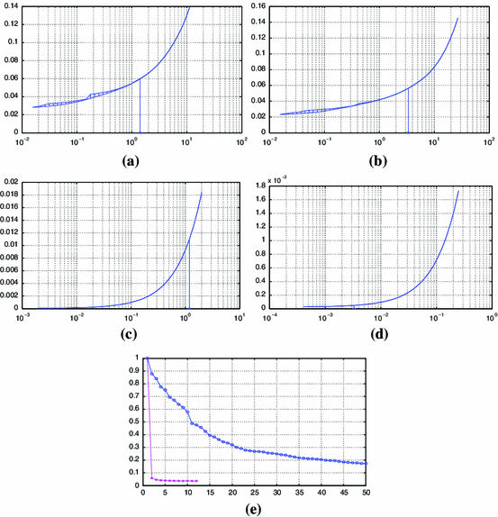

  

  a–d Lower and upper envelopes of $\{\phi _{\kappa }(x_{\kappa _\mathrm{w}}(\kappa )):\kappa _\mathrm{w}\in G\}$ versus $\kappa$, experiments A–D. Asterisks on the $\kappa$-axes: penalties resulting in the smallest combined relative recovery errors. e values of $\phi _{1/8}(x_t)$ versus iteration number $t$ with $z_t^{\prime }$ included (asterisks) and not included (circles) into $Z_t$

• An attractive feature of the proposed approach is the possibility to extract from a single run, the working value of the penalty being $\kappa _\mathrm{w}$, suboptimal solutions $x_{\kappa _\mathrm{w}}(\kappa )$ for a bunch of instances of (9) differing from each other by the values of the penalty $\kappa$. The related question is, of course, how good, in terms of the objective $\phi _{\kappa }(\cdot )$, are the “byproduct” suboptimal solutions $x_{\kappa _\mathrm{w}}(\kappa )$ as compared to those obtained when $\kappa$ is the working value of the penalty. In our experiments, the “byproduct” solutions were pretty good, as can be seen from plots (a)—(c) on Fig. 1, where we see the upper and the lower envelopes of the values of $\phi _{\kappa }$ at the approximate solutions $x_{\kappa _\mathrm{w}}(\kappa )$ obtained from different working values $\kappa _\mathrm{w}$ of the penalty. In spite of the fact that in our experiments the ratios $\kappa /\kappa _\mathrm{w}$ could be as small as $1/8$ and as large as $8$, we see that these envelopes are pretty close to each other, and, as an additional bonus, are merely indistinguishable in a wide neighborhood of the best (resulting in the best recovery) value of the penalty (on the plots, this value is marked by asterisk).

Finally, we remark that in experiments A, B, where the mapping $\mathcal{A}$ is heavily ill-conditioned (see Table 3), TV regularization yields moderate (just about 25 %) improvement in the combined relative recovery error as compared to the one of the trivial recovery (“observations as they are”), in spite of the relatively low ($\sigma =0.05$) observation noise. In contrast to this, in the experiments C, D, where $\mathcal{A}$ is well-conditioned, TV regularization reduces the error by 80 % in experiment C ($\sigma =0.15$) and by 72 % in experiment D ($\sigma =0.4$), see Fig. 2.

Fig. 2

Experiments C, D

Appendix

1.1 Proof of Theorem 1

Define $\epsilon _t=f(x_t)-f^t_*$. When invoking convexity of $f$ and the definition (16), (17) of $f^t_*$, we have

$$\begin{aligned} \langle f'(x_t),x^+_t-x_t\rangle =f_{*,t}-f(x_t)\le f^t_{*}-f(x_t)\;(\le f_*-f(x_t)). \end{aligned}$$

(38)

Observing that for a generic GC algorithm we have (cf. (14), (15)) $f(x_{t+1})\le f(x_t+\gamma _t(x_t^+-x_t)), \gamma _t={2\over t+1}$, and invoking (12), we have

$$\begin{aligned} f(x_{t+1})&\le f(x_t)+\gamma _t\langle f'(x_t),x_t^+-x_t\rangle +{L\over 2} \gamma _t^2\Vert x^+_t-x_t\Vert _X^2 \nonumber \\&\le f(x_t)-\gamma _t(f(x_t)-f^t_*) + {\small \frac{1}{2}}L\gamma _t^2, \end{aligned}$$

(39)

where the concluding $\le$ is due to (38). Since $f_*^{t+1}\ge f_*^{t}$, it follows that

$$\begin{aligned} \epsilon _{t+1}\le f(x_{t+1})-f^{t}_*\le (1-\gamma _t)\epsilon _t+{\small \frac{1}{2}}L\gamma _t^2, \end{aligned}$$

whence

$$\begin{aligned} \epsilon _{t+1}&\le \epsilon _1\prod _{i=1}^t (1-\gamma _i) + {\small \frac{1}{2}}L\sum _{i=1}^t \gamma _i^2\prod _{k=i+1}^t (1-\gamma _k)\nonumber \\&= 2L\sum _{i=1}^t (i+1)^{-2}\prod _{k=i+1}^t (1-{2\over k+1}), \end{aligned}$$

where, by convention, $\prod _{k=t+1}^t=1$. Noting that $\prod _{k=i+1}^t(1-{2\over k+1})=\prod _{k=i+1}^t {k-1\over k+1}= {i(i+1)\over t(t+1)},\;\;\;i=1,\ldots ,t,$ we get

$$\begin{aligned} \epsilon _{t+1}\le 2L\sum _{i=1}^t {i(i+1)\over (i+1)^{2}t(t+1)}\le {2L t\over (t+1)^2}\le {2L (t+2)^{-1}}, \end{aligned}$$

(40)

what is (18).$\square$

1.2 Proof of Theorem 2

The proof, up to minor modifications, goes back to [22], see also [19, 26]; we provide it here to make the paper self-contained. W.l.o.g. we can assume that we are in the nontrivial case (see description of the algorithm).

$\mathbf{1}^0$.:

As it was explained when describing the method, whenever stage $s$ takes place, we have $0<\rho _1\le \rho _s\le \rho _*$, and $\rho _{s-1}<\rho _s$, provided $s>1$. Therefore by the termination rule, the output $\bar{\rho }, \bar{x}$ of the algorithm, if any, satisfies $\bar{\rho }\le \rho _*, f(\bar{x})\le \epsilon$. Thus, (i) holds true, provided that the algorithm does terminate. Thus, all we need is to verify (ii) and (iii).

$\mathbf{2}^0$.:

Let us prove (ii). Let $s\ge 1$ be such that stage $s$ takes place. Setting $X=K[\rho _s]$, observe that $X-X\subset \{x\in E:\Vert x\Vert \le 2\rho _s\}$, whence $\Vert \cdot \Vert \le 2\rho _s\Vert \cdot \Vert _X$, and therefore the relation (4) implies the validity of (12) with $L=4\rho _s^2L_f$. Now, if stage $s$ does not terminate in course of some number $t$ steps, then, in the notation from the description of the algorithm, $f(\bar{x}_t)>\epsilon$ and $f_*^t<{3\over 4}f(\bar{x}_t)$, whence $f(\bar{x}_t)-f_*^t> \epsilon /4$. By Theorem 1.ii, the latter is possible only when $4.5L/(t-2)>\epsilon /4$. Thus, $t\le \max \left[ 5,2+{72\rho _s^2L_f\over \epsilon }\right]$. Taking into account that $\rho _s\le \rho _*$, (ii) follows.

$\mathbf{3}^0$.:

Let us prove (iii). This statement is trivially true when the number of stages is 1. Assuming that it is not the case, let $S\ge 1$ be such that the stage $S+1$ takes place. For every $s=1,\ldots ,S$, let $t_s$ be the last step of stage $s$, and let $u_s, \ell ^s(\cdot )$ be what in the notation from the description of stage $s$ was denoted $f(\bar{x}_{t_s})$ and $\ell ^{t_s}(\rho )$. Thus, $u_s>\epsilon$ is an upper bound on ${\mathop {\hbox {Opt}}}(\rho _s), \ell _s{:=}\ell ^s(\rho _s)$ is a lower bound on ${\mathop {\hbox {Opt}}}(\rho _s)$ satisfying $\ell _s\ge 3u_s/4$, and $\ell ^s(\cdot )$ is a piecewise linear convex in $\rho$ lower bound on ${\mathop {\hbox {Opt}}}(\rho ), \rho \ge 0$, and $\rho _{s+1}>\rho _s$ is the smallest positive root of $\ell ^s(\cdot )$. Let also $-g_s$ be a subgradient of $\ell ^s(\cdot )$ at $\rho _s$. Note that $g_s>0$ due to $\rho _{s+1}>\rho _s$ combined with $\ell ^s(\rho _s)>0, \ell ^s(\rho _{s+1})=0$, and by the same reasons combined with convexity of $\ell ^s(\cdot )$ we have

$$\begin{aligned} \rho _{s+1}-\rho _s\ge \ell _s/g_s, \end{aligned}$$

(41)

and, as we have seen,

$$\begin{aligned} 1\le s\le S\Rightarrow \left\{ \begin{array}{ll} (a)&{}u_s>\epsilon ,\\ (b)&{}u_s\ge {\mathop {\hbox {Opt}}}(\rho _s)\ge \ell _s\ge {3\over 4}u_s,\\ (c)&{}\ell _s-g_s(\rho -\rho _s) \le {\mathop {\hbox {Opt}}}(\rho ),\,\rho \ge 0.\\ \end{array}\right. \!. \end{aligned}$$

(42)

Assuming $1<s\le S$ and applying (41), we get $\rho _s-\rho _{s-1}\ge {3\over 4}u_{s-1}/g_{s-1}$, whence, invoking (42),

$$\begin{aligned} u_{s-1}\ge {\mathop {\hbox {Opt}}}(\rho _{s-1})\ge \ell _s+g_s[\rho _{s-1}-\rho _s]\ge {3\over 4}u_s+{3\over 4}u_{s-1}{g_s\over g_{s-1}}. \end{aligned}$$

The resulting inequality implies that ${u_s\over u_{s-1}}+{g_s\over g_{s-1}}\le {4\over 3}$, whence ${u_sg_s\over u_{s-1}g_{s-1}}\le (1/4)(4/3)^2=4/9$. It follows that

$$\begin{aligned} \sqrt{u_sg_s}\le (2/3)^{s-1}\sqrt{u_1g_1}, \,\,1\le s\le S. \end{aligned}$$

(43)

Now, since the first iterate of the first stage is $0$, we have $u_1\le f(0)$, while (42) applied with $s=1$ implies that $f(0)={\mathop {\hbox {Opt}}}(0)\ge \ell _1+\rho _1g_1\ge \rho _1g_1$, whence $u_1g_1\le f(0)/\rho _1=d$. Further, by (41) $g_s\ge \ell _s/(\rho _{s+1}-\rho _s)\ge \ell _s/\rho _*\ge {3\over 4} u_s/\rho _*$, where the concluding inequality is given by (42). We see that $u_sg_s\ge {3\over 4}u_s^2/\rho _*\ge {3\over 4}\epsilon ^2/\rho _*$. This lower bound on $u_sg_s$ combines with the bound $u_1g_1\le d$ and with (43) to imply that

$$\begin{aligned} \epsilon \le \sqrt{4/3}(2/3)^{s-1}\sqrt{d\rho _*},\,1\le s\le S. \end{aligned}$$

Finally observe that by the definition of $\rho _*$ and due to the fact that $\Vert x[f'(0)]\Vert =1$ in the nontrivial case, we have

$$\begin{aligned} 0&\le f(\rho _*x[f'(0)])\le f(0)+\rho _*\langle f'(0),x[f'(0)]\rangle +{1\over 2}L_f\rho _*^2\nonumber \\&= f(0)-\rho _*d+{\small \frac{1}{2}}L_f\rho _*^2 \end{aligned}$$

(we have used (4) and the definition of $d$), whence $\rho _*d\le f(0)+{\small \frac{1}{2}}L_f\rho _*^2$ and therefore

$$\begin{aligned} \epsilon \le \sqrt{4/3}(2/3)^{s-1}\sqrt{f(0)+{\small \frac{1}{2}}L_f\rho _*^2},\,1\le s\le S. \end{aligned}$$

Since this relation holds true for every $S\ge 1$ such that the stage $S+1$ takes place, (iii) follows. $\square$

1.3 Proof of Theorem 3

By definition of $z_t$ we have $z_t\in K^+$ for all $t$ and $F(0)=F(z_1)\ge F(z_2)\ge \ldots$, whence $r_t\le D_*$ for all $t$ by Assumption A. Besides this, $r_*\le D_*$ as well. Let now $\epsilon _t=F(z_t)-F_*$, $z_t=[x_t;r_t]$, and let $z^+_t=[x^+_t,r^+_t]$ be a minimizer, as given by Lemma 1, of the linear form $\langle F'(z_t),z\rangle$ of $z\in E^+$ over the set $K^+[r_*]=\{[x;r]: x\in K,\Vert x\Vert \le r\le r_*\}$. Recalling that $F'(z_t)=[f'(x_t);\kappa ]$ and that $r_t\le D_*\le \bar{D}$, Lemma 1 implies that $z^+_t\in \Delta (z_t)$. By definition of $z_t^+$ and convexity of $F$ we have

$$\begin{aligned} \begin{array}{rcl} \langle [f'(x_t);\kappa ],z_t-z_t^+\rangle &{}=&{}\langle f'(x_t),x_t-x_t^+\rangle +\kappa (r_t-r_t^+)\\ &{}\ge &{} \langle f'(x_t),x_t-x_*\rangle +\kappa (r_t-r_*)\\ &{}=&{} \langle F'(z_t),\,z_t-z_*\rangle \ge F(z_t)-F(z_*) =\epsilon _t.\\ \end{array} \end{aligned}$$

Invoking (12), it follows that for $0\le s\le 1$ one has

$$\begin{aligned} F(z_t+s(z_t^+-z_t))&\le F(z_i)+s\langle [f'(x_t);\kappa ],z_t^+-z_t\rangle +{L_f s^2\over 2}\Vert x(z_t^+)-x(z_t)\Vert ^2\\&\le F(z_t)-s\epsilon _t +{\small \frac{1}{2}}L_f s^2(r_t+D_*)^2 \end{aligned}$$

using that $\Vert x(z_t^+)\Vert \le r_t^+$ and $\Vert x(z^t)\Vert \le r_t$ due to $z_t^+,z_t\in K^+$, and that $r_t^+\le r_*\le D_*$. By (24) we have

$$\begin{aligned} F(z_{t+1})\le \min _{0\le s\le 1}F(z_t+s(z_t^+-z_t))\le F(z_t)+\min \limits _{0\le s\le 1} \left\{ -s\epsilon _t +{\small \frac{1}{2}}L_f s^2(r_t+D_*)^2\right\} , \end{aligned}$$

and we arrive at the recurrence

$$\begin{aligned} \epsilon _{t+1}\le \epsilon _t-\left\{ \begin{array}{ll}{\epsilon _t^2\over 2L_f (r_t+D_*)^2},&{}\epsilon _t\le L_f (r_t+D_*)^2\\ \epsilon _t-{\small \frac{1}{2}}L_f (r_t+D_*)^2,&{}\epsilon _t> L_f (r_t+D_*)^2\\ \end{array}\right. , t=1,2,\ldots \end{aligned}$$

(44)

When $t=1$, this recurrence, in view of $z_1=0$, implies that $\epsilon _2\le {\small \frac{1}{2}}L_fD_*^2$. Let us show by induction in $t\ge 2$ that

$$\begin{aligned} \epsilon _{t}\le \bar{\epsilon }_t{:=}{8L_f D_*^2\over t+14},\,t=2,3,\ldots \end{aligned}$$

(45)

thus completing the proof. We have already seen that (45) is valid for $t=2$. Assuming that (45) holds true for $t=k\ge 2$, we have $\epsilon _{k}\le {\small \frac{1}{2}}L_f D_*^2$ and therefore $\epsilon _{k+1}\le \epsilon _{k}-{1\over 8L_f D_*^2}\epsilon _{k}^2$ by (44) combined with $0\le r_k\le D_*$. Now, the function $s-{1\over 8L_f D_*^2}s^2$ is nondecreasing on the segment $0\le s\le 4L_f D_*^2$ which contains $\bar{\epsilon }_k$ and $\epsilon _k\le \bar{\epsilon }_k$, whence

$$\begin{aligned} \epsilon _{k+1}&\le \epsilon _{k}-{1\over 8L_f D_*^2}\epsilon _{k}^2\le \bar{\epsilon }_{k}-{1\over 8L_f D_*^2}\bar{\epsilon }_{k}^2 = \left[ {8L_f D_*^2\over k+14}\right] -{1\over 8L_f D_*^2}\left[ {8L_f D_*^2\over k+14}\right] ^2\\&= {8L_f D_*^2(k+13)\over (k+14)^2}\le {8L_f D_*^2\over (k+1)+14}, \end{aligned}$$

so that (45) holds true for $t=k+1$. $\square$

1.4 Proofs for Section 6

As we have already explained, (31) is solvable, so that $z$ is well defined. Denoting by $(s_*,r_*)$ an optimal solution to (31) produced, along with $z$, by our solver, note that the characteristic property of $z$ is the relation

$$\begin{aligned} (s_*,r_*)\in \mathop {\mathrm{Argmax}}_{s,r}\{s+\langle z, Pr-s\eta \rangle : 0\le r\le \mathbf {e}\}. \end{aligned}$$

Since the column sums in $P$ are zeros and the sum of entries in $\eta$ is zero, the above characteristic property of $z$ is preserved when passing from $z$ to $\bar{z}$, so that we may assume from the very beginning that $z=\bar{z}$ is a zero mean image. Now, $P=[Q,-Q]$, where $Q$ is the incidence matrix of the network obtained from $G$ by eliminating backward arcs. Representing a flow $r$ as $[r_f;r_b]$, where the blocks are comprised, respectively, of flows in the forward and backward arcs, and passing from $r$ to $\rho =r_f-r_b$, our characteristic property of $z$ clearly implies the relation

$$\begin{aligned} (s_*,\;\rho _*{:=}r_{*\,f}-r_{*\,b})\in \mathop {\mathrm{Argmax}}_{s,\rho }\{\underbrace{s+\langle z,Q\rho -s\eta \rangle }_{\psi (s,\rho )}:\Vert \rho \Vert _\infty \le 1\}. \end{aligned}$$

(46)

By the optimality conditions in linear programming it follows that

$$\begin{aligned} \begin{array}{ll} (a)&{}\langle z,\eta \rangle =1,\\ (b)&{}\Vert \rho _*\Vert _\infty \le 1,\\ (c)&{}(Q^Tz)_\gamma =\left\{ \begin{array}{ll}\le 0, &{}[\rho _*]_\gamma =-1,\\ =0,&{}[\rho _*]_\gamma \in (-1,1),\\ \ge 0,&{}[\rho _*]_\gamma =1,\\ \end{array}\right. \ \hbox {for all forward arcs}\ \gamma ,\\ (d)&{}Q\rho _*=s_*\eta .\\ \end{array} \end{aligned}$$

(47)

Indeed, $(a)$ stems from the fact that $\psi (s,\rho )$, which is affine in $s$, is above bounded, so that the coefficient at $s$ in $\psi$ should be zero; $(b)$ is the constraint in the maximization problem in (46) to which $(s_*,\rho _*)$ is an optimal solution; $(c)$ is the optimality condition for the same problem w.r.t. the $\rho$-variable; and $(d)$ expresses the fact that $(s_*,r_*)$ is feasible for (31). (47.$d$) and (47.$a$) imply that $\langle Q^Tz,\rho _*\rangle =s_*$, while (47.$c$) says that $\langle Q^Tz,\rho _*\rangle = \Vert Q^Tz\Vert _1$, and $s_*=\Vert Q^Tz\Vert _1$. By (47.$a$) $z\ne 0$, and thus $z$ is a nonzero image with zero mean; recalling what $Q$ is, the first $n(n-1)$ entries in $Q^Tz$ form $\nabla _i z$, and the last $n(n-1)$ entries form $\nabla _jz$, so that $\Vert Q^Tz\Vert _1={\hbox {TV}}(z)$. The gradient field of a nonzero image with zero mean cannot be identically zero, whence ${\hbox {TV}}(z)=\Vert Q^Tz\Vert _1=s_*>0$. Thus $x[\eta ]=-z/{\hbox {TV}}(z)=-z/s_*$ is well defined and ${\hbox {TV}}(x[\eta ])=1$, while by (47.$a$) we have $\langle x[\eta ],\eta \rangle =-1/s_*$. Finally, let $x\in {\mathcal{T}\mathcal{V}}$, implying that $Q^Tx$ is the concatenation of $\nabla _ix$ and $\nabla _jx$ and thus $\Vert Q^Tx\Vert _1={\hbox {TV}}(x)\le 1$. Invoking (47.$b,d$), we get $-1\le \langle Q^Tx,\rho ^*\rangle =\langle x, Q\rho _*\rangle =s_*\langle x,\eta \rangle$, whence $\langle x,\eta \rangle \ge -1/s_*=\langle x[\eta ],\eta \rangle$, meaning that $x[\eta ]\in {\mathcal{T}\mathcal{V}}$ is a minimizer of $\langle \eta ,x\rangle$ over $x\in {\mathcal{T}\mathcal{V}}$. $\square$

In the sequel, for a real-valued function $x$ defined on a finite set (e.g., for an image), $\Vert x\Vert _p$ stands for the $L_p$ norm of the function corresponding to the counting measure on the set (the mass of every point from the set is 1). Let us fix $n$ and $x\in M^n_0$ with ${\hbox {TV}}(x)\le 1$; we want to prove that

$$\begin{aligned} \Vert x\Vert _2\le \mathcal{C}\sqrt{\ln (n)} \end{aligned}$$

(48)

with appropriately selected absolute constant $\mathcal{C}$.

$\mathbf{1}^0$. Let $\oplus$ stand for addition, and $\ominus$ for subtraction of integers modulo $n$; $p\oplus q=(p+q) \,\hbox {mod} \,n\in \{0,1,\ldots ,n-1\}$ and similarly for $p\ominus q$. Along with discrete partial derivatives $\nabla _i x, \nabla _jx$, let us define their periodic versions $\widehat{\nabla }_ix, \widehat{\nabla }_jx$:

$$\begin{aligned} \widehat{\nabla }_ix(i,j)&= x(i\oplus 1,j)-x(i,j):\Gamma _{n,n}\rightarrow {\mathbf {R}},\,\, \widehat{\nabla }_jx(i,j)\nonumber \\&= x(i,j\oplus 1)-x(i,j):\Gamma _{n,n}\rightarrow {\mathbf {R}}, \end{aligned}$$

same as periodic Laplacian $\widehat{\Delta } x$:

$$\begin{aligned} \widehat{\Delta } x=x(i,j)-{1\over 4}\left[ x(i\ominus 1,j){+}x(i\oplus 1,j)+x(i,j\ominus 1) +x(i,j\oplus 1)\right] :\Gamma _{n,n}{\rightarrow }{\mathbf {R}}. \end{aligned}$$

For every $j, 0\le j<n$, we have $\sum _{i=0}^{n-1} \widehat{\nabla }_ix(i,j)=0$ and $\nabla _ix(i,j)=\widehat{\nabla }_ix(i,j)$ for $0\le i<n-1$, whence $\sum _{i=0}^{n-1}|\widehat{\nabla }_i(x)|\le 2\sum _{i=0}^{n-1}|\nabla _ix(i,j)|$ for every $j$, and thus $\Vert \widehat{\nabla }_ix\Vert _1\le 2\Vert \nabla _ix\Vert _1$. Similarly, $\Vert \widehat{\nabla }_jx\Vert _1\le 2\Vert \nabla _jx\Vert _1$, and we conclude that

$$\begin{aligned} \Vert \widehat{\nabla }_ix\Vert _1+\Vert \widehat{\nabla }_jx\Vert _1\le 2. \end{aligned}$$

(49)

$\mathbf{2}^0$. Now observe that for $0\le i,j<n$ we have

$$\begin{aligned} \begin{array}{rcl} x(i,j)&{}=&{}x(i\ominus 1,j)+\widehat{\nabla }_ix(i\ominus 1,j)\\ x(i,j)&{}=&{}x(i\oplus 1,j)-\widehat{\nabla }_ix(i,j)\\ x(i,j)&{}=&{}x(i,j\ominus 1)+\widehat{\nabla }_jx(i,j\ominus 1)\\ x(i,j)&{}=&{}x(i,j\oplus 1)-\widehat{\nabla }_jx(i,j)\\ \end{array} \end{aligned}$$

whence

$$\begin{aligned} \widehat{\Delta } x(i,j)={1\over 4}\left[ \widehat{\nabla }_ix(i\ominus 1,j)- \widehat{\nabla }_ix(i,j)+\widehat{\nabla }_jx(i,j\ominus 1)- \widehat{\nabla }_jx(i,j)\right] \end{aligned}$$

(50)

Now consider the following linear mapping from $M^n\times M^n$ into $M^n$:

$$\begin{aligned} B[g,h](i,j)={1\over 4}\left[ g(i\ominus 1,j)-g(i,j)+h(i,j\ominus 1) -h(i,j)\right] ,\,[i;j]\in \Gamma _{n,n}. \end{aligned}$$

(51)

From this definition and (50) it follows that

$$\begin{aligned} \widehat{\Delta }x=B[\widehat{\nabla }_ix,\widehat{\nabla }_jx]. \end{aligned}$$

(52)

Let for $u\in M^n, {\hbox {DFT}}[u]$ stand for the 2D Discrete Fourier Transform of $u$:

$$\begin{aligned} {\hbox {DFT}}[u](p,q)=\sum _{0\le r,s<n} u(r,s)\exp \{-2\pi \imath (pr+qs)/n\},\,[p;q]\in \Gamma _{n,n}. \end{aligned}$$

Note that every image $u$ with zero mean is the periodic Laplacian of another, uniquely, defined, image $X[u]$ with zero mean, with $X[u]$ given by its Fourier transform

$$\begin{aligned} {\hbox {DFT}}[X[u]](p,q)&= Y[u](p,q){:=}\left\{ \begin{array}{ll}0,&{}p=q=0\\ {{\hbox {DFT}}[u](p,q)\over D(p,q)}, &{}0\ne [p;q]\in \Gamma _{n,n}\\ \end{array}\right. \!\!,\,[p;q]\in \Gamma _{n,n},\nonumber \\ D(p,q)&= 1-{1\over 2}[\cos (2\pi p/n)+\cos (2\pi q/n)],\,\,[p;q]\in \Gamma _{n,n}. \end{aligned}$$

(53)

Indeed, representing an $n\times n$ image $x(\mu ,\nu ),$ $0\le \mu ,\nu <n$, as a Fourier sum

$$\begin{aligned} x(\mu ,\nu )=\sum _{0\le p,q<n}c_{p,q}\exp \{2\pi \imath [p\mu /n+q\nu /n]\}, \end{aligned}$$

we get

$$\begin{aligned} \!\!\!\!\!\!\!\!\begin{array}{rcl} \left[ \widehat{\Delta }x\right] (\mu ,\nu )&{}=&{}\sum \limits _{0\le p,q<n}c_{p,q}\bigg [\exp \{2\pi \imath [{p\mu \over n}+{q\nu \over n}]\}\\ &{}&{}-{1\over 4}\exp \{2\pi \imath [{p(\mu \ominus 1)\over n}+{q\nu \over n}]\} - {1\over 4}\exp \{2\pi \imath [{p(\mu \oplus 1)\over n}+{q\nu \over n}]\}\\ &{}&{}-{1\over 4}\exp \{2\pi \imath [{p\mu \over n}+{(q\ominus 1)\nu \over n}]\}-{1\over 4}\exp \{2\pi \imath [{p\mu \over n}+{q(\nu \oplus 1)\over n}]\}\bigg ]\\ &{}=&{} \sum \limits _{0\le p,q<n}c_{p,q}\exp \{2\pi \imath [{p\mu \over n}+{q\nu \over n}]\}\bigg [1-{1\over 4}\exp \{-2\pi \imath {p\over n}\}-{1\over 4}\exp \{2\pi \imath {p\over n}\}\\ &{}&{} -{1\over 4}\exp \{-2\pi \imath {q\over n}\} - {1\over 4}\exp \{2\pi \imath {q\over n}\}\bigg ]\\ &{}=&{}\sum \limits _{0\le p,q<n}\left[ c_{p,q}D(p,q)\right] \exp \{2\pi \imath [{p\mu \over n}+{q\nu \over n}]\},\qquad \end{array} \end{aligned}$$

where

$$\begin{aligned} D(p,q)&= \left[ 1-{1\over 4}\exp \{-2\pi \imath {p\over n}\}-{1\over 4}\exp \{2\pi \imath {p\over n}\}-{1\over 4}\exp \{-2\pi \imath {q\over n}\} - {1\over 4}\exp \{2\pi \imath {q\over n}\}\right] \\&= 1-{1\over 2}\cos (2\pi {p\over n})-{1\over 2}\cos (2\pi {q\over n}),\,\,[p;q]\in \Gamma _{n,n}. \end{aligned}$$

In other words, in the Fourier domain passing from an image to its periodic Laplacian means multiplication of Fourier coefficient $c_{p,q}$ by $D(p,q)$. From the expression for $D(p,q)$ it is immediately seen that $D(p,q)$ is nonzero whenever $(p,q)$ with $0\le p,q<n$ is nonzero. In other words, the periodic Laplacian of a whatever $n\times n$ zero mean image is an image with zero mean (zero Fourier coefficient $(0,0)$), and every image of this type is a periodic Laplacian of another zero mean image described in (53).

In particular, invoking (52), we get

$$\begin{aligned} {\hbox {DFT}}[x]=Y[B[\widehat{\nabla }_ix,\widehat{\nabla }_jx]]. \end{aligned}$$

By Parseval identity, $\Vert {\hbox {DFT}}[x]\Vert _2=n\Vert x\Vert _2$, whence

$$\begin{aligned} \Vert x\Vert _2=n^{-1}\Vert Y[B[\widehat{\nabla }_ix,\widehat{\nabla }_jx]]\Vert _2. \end{aligned}$$

Combining this observation with (49), we see that in order to prove (48), it suffices to check that

(!) Whenever $g,h\in M^n$ are such that

$$\begin{aligned} (g,h)\in G{:=}\{(g,h)\in M^n\times M^n: \Vert g\Vert _1+\Vert h\Vert _1\le 2\}, \end{aligned}$$

we have

$$\begin{aligned} \Vert Y[B[g,h]]\Vert _2\le n\mathcal{C}\sqrt{\ln (n)}. \end{aligned}$$

(54)

$\mathbf{4}^0$. The good news about (!) is that $Y[B[g,h]]$ is linear in $(g,h)$. Therefore, in order to justify (!), it suffices to prove that (54) holds true for the extreme point of $G$, i.e., (a) for pairs where $h\equiv 0$ and $g$ is an image which is equal to 2 at some point of $\Gamma _{n,n}$ and vanishes outside of this point, and (b) for pairs where $g\equiv 0$ and $h$ is an image which is equal to 2 at some point of $\Gamma _{n,n}$ and vanishes outside of this point. Task (b) clearly reduces to task (a) by swapping the coordinates $i,j$ of points from $\Gamma _{n,n}$, so that we may focus solely on task (a). Thus, assume that $g$ is a cyclic shift of the image $2\delta$:

$$\begin{aligned} g(i,j)\equiv 2\delta (i\ominus r,j\ominus s),\,\,\delta (i,j)=\left\{ \begin{array}{ll} 1,&{}[i;j]=[0;0]\\ 0,&{}[i;j]\ne [0;0]\\ \end{array}\right. ,\,[i;j]\in \Gamma _{n,n}. \end{aligned}$$

From (51) it follows that then $B[g,0]$ is a cyclic shift of $B[2\delta ,0]$, whence $|{\hbox {DFT}}[B[g,0]](p,q)|=|{\hbox {DFT}}[B[2\delta ,0]](p,q)|$ for all $[p;q]\in \Gamma _{n,n}$, which, by (53), implies that $|Y[B[g,0]](p,q)|=|Y[B[2\delta ,0]](p,q)|$ for all $[p;q]\in \Gamma _{n,n}$. The bottom line is that all we need is to verify that (54) holds true for $g=2\delta ,h=0$, or, which is the same, that with

$$\begin{aligned} y(p,q)={(1-\exp \{2\pi \imath p/n\})\over 2[1-{1\over 2}[\cos (2\pi p/n)+\cos (2\pi q/n)]]} \end{aligned}$$

(55)

where the right hand side by definition is $0$ at $p=q=0$, it holds

$$\begin{aligned} C_n{:=}\sum _{p,q=0}^{n-1} |y(p,q)|^2 \le n^2\mathcal{C}^2\ln (n). \end{aligned}$$

Now, (55) makes sense for all $[p;q]\in {\mathbf {Z}}^2$ (provided that we define the right hand side as zero at all points of ${\mathbf {Z}}^2$ where the denominator in (55) vanishes, that is, at all point where $p,q$ are integer multiples of $n$) and defines $y$ as a double-periodic, with periods $n$ in $p$ and in $q$, function of $[p;q]$. Therefore, setting $m=\lfloor n/2\rfloor \ge 1$ and $W=\{[p;q]\in {\mathbf {Z}}^2: -m\le p,q<n-m\}$, we have

$$\begin{aligned} C_n=\sum _{0\ne [p;q]\in W} |y(p,q)|^2=\sum _{[p;q]\in W} {|1-\exp \{2\pi \imath p/n\}|^2\over 4|1-{1\over 2}[\cos (2\pi p/n)+\cos (2\pi q/n)]|^2}. \end{aligned}$$

Setting $\rho (p,q)=\sqrt{p^2+q^2}$, observe that when $0\ne [p;q]\in W$, we have $|1-\exp \{2\pi \imath p/n\}|\le C_1n^{-1}\rho (p,q)$ and $2[1-{1\over 2}[\cos (2\pi p/n)+\cos (2\pi q/n)]]\ge C_2n^{-2}\rho ^2(p,q)$ with positive absolute constants $C_1,C_2$, whence

$$\begin{aligned} C_n\le (C_1/C_2)^2\sum _{0\ne [p;q]\in W} n^2\rho ^{-2}(p,q). \end{aligned}$$

With appropriately selected absolute constant $C_3$ we have

$$\begin{aligned} \sum _{0\ne [p;q]\in W} \rho ^{-2}(p,q)\le C_3\int \limits _{1}^n r^{-2}rdr=C_3\ln (n). \end{aligned}$$

Thus, $C_n\le (C_1/C_2)^2C_3n^2\ln (n)$, meaning that (54), and thus (48), holds true with $\mathcal{C}=\sqrt{C_3}C_1/C_2$. $\square$

We are very grateful to Referees for their reading of the manuscript and thoughtful comments.

We have included after Theorem 2 a comment on comparison of the proposed parametric optimization algorithm with that based on bisection. However, we finally decided not to include the numerical comparison. Note that including such experiment would require explaining in some detail what the “bisection” algorithm is and how is it implemented, what would make the manuscript which is already too long with respect to the size requirements of the Mathematical Programming even longer.

We would like to thank Referee 2 for detailed and clarifying explanations of his comments on the initial manuscript. Some comments of Referee 2 concern notation we have not modified in our revision. Since his requests do not seem to be compulsory and the final decision is left to us, we have modified some (e.g., we replaced $D^+$ with $\bar{D}$) but preferred to keep other unchanged.

In what follows we provide our answers to other questions raised in his detailed report.

• $6.16^*$ ...I would suggest that the authors simply say, when introducing (12), that is it is implied by (4) but more general, to give some hint about why they are mentioning it

  We have added a small comment after display (12) to make clear the choice of the norm $\Vert \cdot \Vert _X$ here

• $11.9^*$ ...some readers might be more familiar with a statement like “$\mathcal{A}$ has full column rank,” or “$\mathcal{A}$ has a trivial nullspace,” etc.

  We think that for a linear operator (which, in our case, may not be a matrix) a commonly adopted terminology is indeed “$\mathcal{A}$ has a trivial nullspace,” or “$\mathcal{A}$ has a trivial kernel”, what is the exact wording of $\mathrm{Ker}(\mathcal{A})=\{0\}$.

• $11.19^*$ ...but I think it would suffice to simply note in the text that the given value $\sum |\lambda _\zeta |\rho$ is an upper bound on $\Vert x\Vert$ for $x$ in the given form.

  Thank you, we have added a comment in this sense after display (29).

• $30.5^*$ ...I’ll say that the authors are practicing a false economy in not giving a more complete explanation, and that at the least, “we immediately see” should be “one can show”

  Thank you for insisting, you are probably right—we have reproduced in the text our answer to the corresponding comment on the previous version of the manuscript.

References

Andersen, E.D., Andersen, K.D.: The MOSEK optimization tools manual. http://www.mosek.com/fileadmin/products/6_0/tools/doc/pdf/tools.pdf
Bach, F., Jenatton, R., Mairal, J., Obozinski, G. et al.: Convex optimization with sparsity-inducing norms. In: Sra, S., Nowozin, S., Wright, S. J. (eds). Optimization for Machine Learning, pp. 19–53. MIT Press
Cai, J.-F., Candes, E.J., Shen, Z.: A singular value thresholding algorithm for matrix completion. SIAM J. Optim. 20(4), 1956–1982 (2008)
Candès, E., Recht, B.: Exact matrix completion via convex optimization. Found. Comput. Math. 9(6), 717–772 (2009)
Cox, B., Juditsky, A., Nemirovski, A.: Dual subgradient algorithms for large-scale nonsmooth learning problems. Math. Program. 1–38 (2013). doi:10.1007/s10107-013-0725-1
Demyanov, V., Rubinov, A.: Approximate Methods in Optimization Problems. American Elsevier, Amsterdam (1970)
Dudik, M., Harchaoui, Z., Malick, J.: Lifted coordinate descent for learning with trace-norm regularization. In: AISTATS (2012)
Dunn, J.C., Harshbarger, S.: Conditional gradient algorithms with open loop step size rules. J. Math. Anal. Appl. 62(2), 432–444 (1978)
Frank, M., Wolfe, P.: An algorithm for quadratic programming. Naval Res. Logist. Q. 3, 95–110 (1956)
Goldfarb, D., Ma, S., Wen, Z.: Solving low-rank matrix completion problems efficiently. In: Proceedings of 47th Annual Allerton Conference on Communication, Control, and Computing (2009)
Harchaoui, Z., Douze, M., Paulin, M., Dudik, M., Malick, J.: Large-scale image classification with trace-norm regularization. In: CVPR (2012)
Harchaoui, Z., Juditsky, A., Nemirovski, A.: Conditional gradient algorithms for machine learning. In: NIPS Workshop on Optimization for Machine Learning. http://opt.kyb.tuebingen.mpg.de/opt12/papers.html (2012)
Hastie, T., Tibshirani, R., Friedman, J.: The Elements of Statistical Learning. Springer Series in Statistics. Springer, Berlin (2008)
Hazan, E.: Sparse approximate solutions to semidefinite programs. In: Proceedings of the 8th Latin American Conference Theoretical Informatics, pp. 306–316 (2008)
Hearn, D., Lawphongpanich, S., Ventura, J.: Restricted simplicial decomposition: computation and extensions. Math. Program. Stud. 31, 99–118 (1987)
Holloway, C.: An extension of the Frank-Wolfe method of feasible directions. Math. Program. 6, 14–27 (1974)
Jaggi, M.: Revisiting Frank-Wolfe: projection-free sparse convex optimization. In: ICML (2013)
Jaggi, M., Sulovsky, M.: A simple algorithm for nuclear norm regularized problems. In: ICML (2010)
Juditsky, A., Karzan, F.K., Nemirovski, A.: Randomized first order algorithms with applications to \(\ell _1\)-minimization. Math. Program. 142(1–2), 269–310 (2013)
Juditsky, A., Nemirovski, A.: First order methods for nonsmooth large-scale convex minimization, i: general purpose methods; ii: utilizing problem’s structure. In: Sra, S., Nowozin, S., Wright, S. (eds). Optimization for Machine Learning, pp. 121–184. The MIT Press, Cambridge (2012)
Lan, G.: An optimal method for stochastic composite optimization. Math. Program. 133(1–2), 365–397 (2012)
LemarÃchal, C., Nemirovskii, A., Nesterov, Y.: New variants of bundle methods. Math. Program. 69(1–3), 111–147 (1995)
Ma, S., Goldfarb, D., Chen, L.: Fixed point and bregman iterative methods for matrix rank minimization. Math. Program. 128, 321–353 (2011)
Nemirovski, A., Onn, S., Rothblum, U.G.: Accuracy certificates for computational problems with convex structure. Math. Oper. Res. 35(1), 52–78 (2010)
Nemirovski, A.S., Yudin, D.B.: Problem Complexity and Method Efficiency in Optimization. Wiley-Interscience, New York (1983)
Nesterov, Y.: Introductory Lectures on Convex Optimization: A Basic Course. Kluwer, Berlin (2003)
Nesterov, Y.: Gradient methods for minimizing composite functions. Math. Program. 140(1), 125–161 (2013)
Nesterov, Y., Nemirovski, A.: On first-order algorithms for l 1/nuclear norm minimization. Acta Numer. 22, 509–575 (2013)
Pshenichnyj, B., Danilin, Y.: Numerical Methods in Extremal Problems. Mir, Moscow (1978)
Recht, B., Fazel, M., Parrilo, P.: Guaranteed minimum-rank solutions of linear matrix equations via nuclear norm minimization. SIAM Rev. 52(3), 471–501 (2010)
Recht, B., Ré, C.: Parallel stochastic gradient algorithms for large-scale matrix completion. Math. Program. Comput. 5(2), 201–226 (2013)
Rudin, L., Osher, S., Fatemi, E.: Nonlinear total variation based noise removal algorithms. Phys. D 60 (1992)
Shalev-Shwartz, S., Gonen, A., Shamir, O.: Large-scale convex minimization with a low-rank constraint. In: ICML (2011)
Sra, S., Nowozin, S., Wright, S.J.: Optimization for Machine Learning. MIT Press, Cambridge (2010)
Srebro, N., Shraibman, A.: Rank, trace-norm and max-norm. In: COLT (2005)
Ventura, J.A., Hearn, D.W.: Restricted simplicial decomposition for convex constrained problems. Math. Program. 59, 71–85 (1993)
Yang, J., Yuan, X.: Linearized augmented lagrangian and alternating direction methods for nuclear norm minimization. Math. Comput. 82(281), 301–329 (2013)
Zhang, X., Yu, Y., Schuurmans, D.: Accelerated training for matrix-norm regularization: a boosting approach. In: NIPS, pp. 2915–2923 (2012)
Zibulevski, M., Narkiss, G.: Sequential subspace optimization method for large-scale unconstrained problems. Technical Report CCIT No 559, Faculty of Electrical engineering, Technion (2005)
Author information
Authors and Affiliations
Corresponding author
Additional information
Research of the first and second authors was supported by the CNRS-Mastodons project GARGANTUA, and the LabEx PERSYVAL-Lab (ANR-11-LABX-0025). Research of the third author was supported by the ONR Grant N000140811104 and NSF Grants DMS 0914785, CMMI 1232623.