Stream runtime verification of real-time event streams with the Striver language

Abstract

In this paper, we study the problem of runtime verification of real-time event streams; in particular, we propose a language to describe monitors for real-time event streams that can manipulate data from rich domains. We propose a solution based on stream runtime verification (SRV), where monitors are specified by describing how output streams of data are computed from input streams of data. SRV enables a clean separation between the temporal dependencies among incoming events and the concrete operations that are performed during the monitoring. Most SRV specification languages assume that all streams share a global synchronous clock and divide time in discrete instants. At each instant every input has a reading, and for every instant the monitor computes an output. In this paper, we generalize the time assumption to cover real-time event streams, but keep the explicit time offsets present in some synchronous SRV languages like Lola. The language we introduce, called Striver, shares with SRV the simplicity and economy of operators, and the separation between the reasoning about time and the computation of data values. The version of Striver in this paper allows expressing future and past dependencies. Striver is a general language that allows expressing for certain time domains other real-time monitoring languages, like TeSSLa, and temporal logics, like STL. We show in this paper translations from other formalisms for (piecewise-constant) real-time signals and timed event streams. Finally, we report an empirical evaluation of an implementation of Striver.

1 Introduction

Runtime verification (RV) is a lightweight formal method that studies the problem of whether a single trace from the system under analysis satisfies a formal specification. Runtime verification is therefore a dynamic technique that considers only the traces observed, in contrast with static verification that must consider all executions of the system. Consequently, runtime verification sacrifices completeness to obtain a readily applicable formal method that can be combined with testing or debugging. Other common use of RV is the formal monitoring of reactive systems to provide explanations of the system behavior dynamically, which can be combined at runtime with corrective measures. See [1, 2] for surveys on RV, and the recent book [3]. Early specification languages proposed in RV were based on temporal logics [4,5,6], regular expressions [7], timed regular expressions [8], rules [9], or rewriting [10]. The approach we propose here is based on stream runtime verification (SRV), pioneered by Lola [11].

Stream runtime verification defines monitors by declaring the dependencies between output streams (results) and input streams (observations from the system). The main idea of SRV is that the same sequence of steps performed during the monitoring of a temporal logic formula can be followed to compute statistics of the input trace, as the temporal dependencies between the inputs and outputs are the same. The only necessary change is to generalize the operations performed from the data collected as input to compute the intermediate results and outputs, which allows computing richer verdicts, following the same steps and data dependencies. The generalization of the outcome of the monitoring process to richer verdict values brings runtime verification closer to monitoring and data stream-processing. See [12,13,14] for further works on SRV. Temporal testers [15], which can be seen as a Boolean SRV description, were later proposed as a similar monitoring technique for LTL. SRV was initially conceived for monitoring synchronous systems, where computation proceeds in cycles.

In the pioneering Lola SRV specification language, writing a specification consists of associating every output stream variable with a defining equation. The intention is that—once the input streams are known—each output variable is mapped to the unique output stream that satisfies its equation. Take, for example, the following Lola specification [11]:

$$\begin{aligned} \begin{array}{l} \texttt { input bool p }\\ \texttt { define int one\_p := if p then 1 else 0 }\\ \texttt { output bool always\_p := p /\ always\_p[-1,true] }\\ \texttt { output int count\_p := one\_p + count\_p [-1,0]} \end{array} \end{aligned}$$

This specification defines one intermediate stream, called one_p, and two output streams, called always_p and count_p. The output stream always_p captures whether the Boolean input stream p was true at every point in the past (that is, the LTL formula ). The stream one_p is 1 when the input p is true and 0 otherwise, which eases the definition of count_p to count the number of times p was true in the past. Offset expressions like count_p[-1,0] or always_p[-1,true] refer to a different position in a stream with a default value when there is no such a position (that is, before the beginning and after then end of the trace). The offset expression count_p[-1,0] refers to stream count_p at the previous position with default value 0 if the referred position falls before the beginning of the trace. Similarly, the offset expression always_p[-1,true] refers to the previous position with default value true. In this paper, we introduce a similar formalism for timed event streams. Our goal is to provide a simple language with few constructs including explicit references to the previous and next position at which some stream contains an event.

Other similar languages for timed event streams are TeSSLa  [16] and RTLola  [17] but both of these preclude to reason explicitly about real-time instants. Instead, TeSSLa and RTLola offer building blocks like stream transformers in the language to describe the temporal dependencies between streams. For this reason we say that Striver is an explicit time SRV formalism.

Striver is a stream-based declarative specification language for timed asynchronous observations, where streams are sequences of timed events. In other words, events in different streams do not necessarily happen at the same time. However, all time-stamps are totally ordered according to a global clock. This is the assumption made in the timed asynchronous model of distributed systems [18]. Striver targets the outline, non-intrusive monitoring of real-time systems. Outline in this context means that the monitor is not intertwined or modifies the system under analysis, but instead runs on its specific infrastructure, with the goal of minimizing the effect of monitoring on the system’s behavior (non-intrusiveness). One of the most important concerns in RV is the usage of resources. The concept of trace length independence refers to the ability of a monitoring algorithm to carry out the online evaluation (processing of input streams to generate output streams) with an amount of memory that can be bounded from the specification and is independent of the length of the trace.

Our intended application is the monitoring and testing of cloud systems and multi-core hardware monitoring, where our time assumption is reasonable. The Elastest project [19] aims at improving the testing of large cloud applications. The Elastest Monitoring Service (EMS) is a component of the Elastest infrastructure that improves the testing capabilities of Elastest. The core of the EMS is an implementation of the algorithms described in this paper.

Notions of time. The concepts of time used in this paper are summarized as follows:

• Synchronous SRV. Time proceeds as sequence of instants, where exactly one event is read in each input stream, and one output event is eventually computed for each output stream. Examples of specification languages that assume a synchronous model of time are Lola [11] and LTL [20].

• Isochronous SRV. The time domain is potentially continuous. Each observation is an event which carries a time-stamp and can happen at any point. However, output streams are updated at periodic intervals (which justifies the name isochronous) or at those instants where there is an event in an input stream. Examples include the periodic stream definitions in RTLola [17].

• Asynchronous SRV. Again, the time domain is potentially continuous time, and time-stamped events can occur at any time. Output streams can contain events at arbitrary points in time, without any period or input event. This requires the engine to generate events at arbitrary instants which justifies the name asynchronous. Examples are Striver  [21] (extended in this paper) and TeSSLa  [16]. RTLola [17] can generate events at periodic times and also at those times at which there is an input event.

Related work. TeSSLa  [16] is a specification language for timed-event streams based on stream transformers (basic building blocks that take streams and define new streams). In contrast, Striver uses a style of specification that expresses the dependency of streams using explicit time offsets, in an approach more aligned to Lola. The seminal paper for TeSSLa  [16] presents the language, and [22] shows asynchronous operational semantics for a simpler fragment of the language (that encapsulates all recursion within the building blocks) that also disallows non-Zeno specifications. We prove in this paper that Striver subsumes TeSSLa (under some assumptions) in the sense that every stream transformer from TeSSLa can be implemented in Striver.

Another similar work is RTLola  [17], which also aims to extend SRV from the synchronous domain to timed streams. In RTLola, defined streams are either computed at predefined periodic instants of time or at the ticking time of input streams. Even though the semantics of RTLola are given informally in [17], RTLola is either input driven or isochronous according to the definition above because output streams can only be generated at periodic times or at time triggered instants. RTLola is very efficient on inputs arriving at high speeds as a typical RTLola specification simply stores input events and computes output events (typically summaries) at regular intervals. However, this sacrifices trace length independence unless there is an assumption on the ratio of arrival of events. Compared to RTLola, in the model of computation of Striver, streams are computed at the specific real-time instants where they are required, resulting in a fully asynchronous SRV system. In this case, Striver is strictly more expressive than RTLola (the version from [17]) because RTLola cannot define properties that must be interpreted at every instant of time (like “there cannot be more than k events in any window of 3 s”) which require to produce events in the output at instants that are neither periodic nor present in the input. It is simple to see that every construct in RTLola can be translated into a few lines of Striver code. Also, asynchronous languages like TeSSLa and Striver can be used more easily to define specifications that are guaranteed to be trace length independent, and be very efficient on inputs with sparse event but occasional heavy bursts.

Signal temporal logic (STL) [23, 24] is a temporal logic for real-time signals based on metric temporal logic (MTL) [25] that is capable of dealing with numeric signals. We show in Sect. 5.2 that Striver can subsume STL over piecewise-constant signals and also generalize the semantics of STL to quantitative data collection over piecewise constant signal inputs.

Data Stream Management Systems (DSMS) [26] allow working with streams of input data by continuously executing queries over stored stream. Typically, DSMS queries are executed periodically and thus they present issues inherent to isochronous approaches. In particular, these systems are sensitive to sparse bursts of events, having to decide whether to buffer a rather large input data and keep the execution period high, or execute with a higher frequency, and waste CPU cycles when there is no data to consume. Also, the evaluation of queries typically comes in two flavors: (1) the ones that are evaluated over a fixed window of time, which may require only bounded resources but restrict the range of observations (for example, in the Continuous Query Language (CQL) developed as part of the STREAM Data Stream Management System [27]); (2) the evaluations that store the whole history (which require unbounded storage). In comparison, one of the main concerns of stream runtime verification is to study rich monitoring languages with formal semantics that know the whole history of the computation and can be evaluated with bounded resources.

Contributions. In summary, the contributions of the paper are:

• 1. The Striver specification language, which generalizes (preserving the separation between data and time) SRV to timed event streams, keeping explicit time offsets, and not using additional building blocks or stream transformers.

• 2. A trace length-independent online algorithm for the past fragment, included in Sect. 4.1, and an online algorithm for the full language, included in Sect. 4.2 (which is not trace length independent in general).

• 3. A comparison between TeSSLa and Striver, which is included in Sect. 5.1.

• 4. An extension of the language to describe sliding windows, in Sect. 5.2, which allows a translation from STL to Striver.

• 5. An empirical evaluation for both the past fragment and the extensions including future dependencies and windows, reported in Sect. 6.

Journal paper. An earlier version of this paper appears in the Proceedings of the 18th International Conference on Runtime Verification (RV’18) [21]. This paper extends [21] including many proofs and additional examples, and more specifically, the following additions:

• An extension of Striver that includes future operators, which involves extending the syntax, type inference system and generalizing the semantics and well-formedness condition.

• The complete proof of trace length independence of the algorithm for the past fragment of Striver presented in [21] and a completely new online algorithm for the fully fledged version of Striver, included in Sect. 4.2.

  This algorithm does not proceed synchronously as the simpler algorithm from but instead accesses each of the streams independently.

• The complete comparison with all operators of the TeSSLa specification language, included in Sect. 5.1.

• A further extension to define truly sliding windows in Striver (windows that span from any two points in the time domain) and the comparison with STL, included in Sect. 5.2. This requires the bounded future fragment of Striver, introduced in the same section.

• An extended empirical evaluation, in Sect. 6, particularly with new experiments to evaluate the extensions of the language.

• A discussion of the language properties in Sect. 7 including a finer-grain analysis on time boundaries, a sketch on how to perform offline monitoring which is a method to achieve trace length independence monitoring provided the appropriate host capabilities.

2 Preliminaries

The keystone of Stream Runtime Verification is to separate two concerns: the temporal dependencies and the data manipulated. The temporal dependencies are used to calculate the order of operations in monitoring algorithms, while the data manipulation describes how to perform each operation. We use here the term data domains to refer to the first-order signatures and structures that allows modeling the data manipulation. The clean separation between temporal dependencies and data domains allows generalizing existing algorithms that monitor temporal logics, from Boolean verdicts to quantitative verdicts, by using data domains richer than Booleans.

2.1 Data domains

We use many-sorted first-order signatures and structures to describe data domains. A signature $\varSigma :\langle \mathcal {S},\mathcal {F}\rangle$ consist on a finite collection of sorts $\mathcal {S}$, and function symbols $\mathcal {F}$ (where each argument of a function has a sort, and the resulting term also has a sort). A simple signature is Booleans, that has only one sort (Bool) with two constants ( $\texttt {true}$ and $\texttt {false}$), binary functions ( , $\mathrel {\vee }$...), unary functions like $\mathclose {\lnot }$, etc. In this paper, we use sort and type interchangeably. A more sophisticated signature is Naturals that consists of two sorts (Nat and Bool), with constant symbols $\mathtt {0}$, $\mathtt {1}$, $\mathtt {2}$...of sort Nat, binary symbols $\mathtt {+}$, $\mathtt {*}$, etc. (of sort $\textit{Nat}\times \textit{Nat}\mathrel {\rightarrow }\textit{Nat}$) as well as predicates $\mathtt {<}$, $\mathtt {\le }$, which take two $\textit{Nat}$ arguments and return a $\textit{Bool}$ with their usual interpretation. We assume that all signatures have equality over all sorts and that every sort (Nat, Bool, Queue, Stack, etc.) is equipped with a ternary symbol $\mathtt {if}\cdot \mathtt {then}\cdot \mathtt {else}\cdot$. In the case of Nat, the $\mathtt {if}\cdot \mathtt {then}\cdot \mathtt {else}\cdot$ symbol has type $\textit{Bool}\times \textit{Nat}\times \textit{Nat}\mathrel {\rightarrow }\textit{Nat}$.

The theories we consider are interpreted. Therefore, for every first-order signature there is a structure where all function symbols have a computational interpretation. That is, every sort S is associated with a domain $D_S$ (a concrete set of values), and each function symbol $\mathtt {f}$ is interpreted as a total computable function $f$, with the given arity and that produces values of the domain of the result given elements of the arguments’ domains. For example, the symbol + can be used to construct an expression of type $\textit{Nat}$ given two expressions of type $\textit{Nat}$, and + is associated with the interpreted function $+$ that computes the sum of two natural numbers. For simplicity, we omit the sort S from $D_S$ (and simply write D) if it is clear from the context.

We will build specifications using stream variables to model input and output streams. Each stream variable is associated with a sort. From the point of view of syntactic expressions, stream variables are used to build atoms. As usual, given a set of sorted atoms A and a signature, the set of terms is the smallest set containing A and closed under the use of function symbols in the signature as term constructors (respecting sorts).

We consider a special time domain $\mathbb {T}$, whose interpretation is a (possibly infinite, possibly dense) totally ordered set. We also require the existence of a superset of the time domain $\mathbb {T}^+$ closed under addition $+$ (which is a total function), and such that the temporal domain $\mathbb {T}$ is an interval of $\mathbb {T}^+$. Usually, time domains contain a minimal element $\bar{0}$, a maximal element $\bar{1}$, or both, to denote the beginning and the end of time. Examples of time domains are $\mathbb {R}_{\ge 0}$, $\mathbb {Q}_{\ge 0}$, and $\mathbb {N}$, with their usual order. Given $t_a,t_b\in \mathbb {T}$, we use $[t_a,t_b]=\{ t \in \mathbb {T} \mid t_a\le t\le t_b\}$, and also $(t_a,t_b)$, $[t_a,t_b)$ and $(t_a,t_b]$ with the usual meaning. We say that a set of time points $S\subseteq \mathbb {T}$ is non-Zeno when it does not contain bounded subsets with infinitely many elements, this is, whenever for every $t_a,t_b\in \mathbb {T}$, the set $S\cap [t_a,t_b]$ is finite.

We extend every domain D into $D_{\mathtt {notick}}$ by including the fresh symbol to indicate when a stream of type D does not contain an event. Additionally, we extend $D_{\mathtt {notick}}$ into $D^\bot$ by including two additional fresh symbols: and . We extend the equality function symbol in the signatures to deal with the introduced constants, where each constant is equal to itself, and different from the other constants and from all elements in the sorts of the underlying signature. The fresh symbols and are used to represent whether a time offset falls off the beginning or the end of the trace. We use $\mathbb {T}_{\texttt {-out}}$ for , $\mathbb {T}_{\texttt {+out}}$ for and $\mathbb {T}_{\texttt {out}}$ for . Similarly, we use $D_{\texttt {-out}}$ for , $D_{\texttt {+out}}$ for and $D_{\texttt {out}}$ for .

A key principle in the design of Striver is that the implementation of data domains is used completely off-the-shelf, so the addition of these new symbols is performed within the Striver engine, and the actual off-the-self data domain implementation only receives actual values from the appropriate domains. Besides equality (which is easily extended as described above), we do not force any function in the theories (like $+$ for example) to handle these new symbols.

2.2 Streams

Monitors observe sequences of events as inputs, where each event contains a data value from its domain and is time-stamped with an increasing time value. We model these sequences as event streams. Given a partial function $f:A\rightharpoondown B$, we use $\textit{dom}(f)$ as the subset of A where f is defined.

Definition 1

(Event stream) An event stream of sort D is a partial function $\eta : \mathbb {T} \rightharpoondown D$ such that $\textit{dom}(\eta )$ does not contain bounded infinite subsets.

The set $\textit{dom}(\eta )$ is called the set of event points of $\eta$. An event stream $\eta$ with a first element can be naturally represented as a timed word:

$$\begin{aligned} s_\eta = (t_0,\eta (t_0))(t_1,\eta (t_1))\dots \in (\textit{dom}(\eta ) \times D)^*, \end{aligned}$$

such that:

• 1. $s_\eta$ is ordered by time ($t_i < t_{i+1}$); and

• 2. the set $\{t \mid (t,d)\in s_\eta \}$ is non-Zeno.

Note that every sequence that is non-Zeno has first element if the time domain has minimum element (or if at least $\textit{dom}(\eta )$ has a minimum element). If $\textit{dom}(\eta )$ does not have a maximum element, we can extend time-words $\eta$ into $\omega$-timed words

$$\begin{aligned} s_\eta = (t_0,\eta (t_0))(t_1,\eta (t_1))\dots \in (\textit{dom}(\eta ) \times D)^\omega . \end{aligned}$$

The set of all event streams over D is denoted by $\mathcal {E}_D$.

We introduce some additional notation for event streams to capture the previous and next event in the stream for a given point in time. Given a stream $\sigma$ and a time instant $t\in \mathbb {T}$, the expression ${{\,\mathrm{{\textit{prev}}}\,}}_{<}(\sigma ,t)$ provides the nearest time instant in the past of t at which $\sigma$ is defined. Similarly, ${{\,\mathrm{{\textit{prev}}}\,}}_{\le }(\sigma ,t)$ returns t if $t\in \textit{dom}(\sigma )$; otherwise, it behaves as ${{\,\mathrm{{\textit{prev}}}\,}}_{<}$. Formally,

The type of ${{\,\mathrm{{\textit{prev}}}\,}}_{<}$ and ${{\,\mathrm{{\textit{prev}}}\,}}_{\le }$ is $\mathcal {E}_D \times \mathbb {T} \mathrel {\rightarrow }\mathbb {T}_{\texttt {-out}}$. These functions can return because $\textit{sup}$ returns when the stream has no events in the interval provided. Note that $\textit{max}(S)$ is well-defined because time is totally ordered and every stream $\sigma$ has a finite number of elements in every given interval. Similarly, given a stream $\sigma$ and a time $t\in \mathbb {T}$, the expression ${{\,\mathrm{{\textit{succ}}}\,}}_{>}(\sigma ,t)$ provides the nearest time instant in the future of t at which s is defined, and ${{\,\mathrm{{\textit{succ}}}\,}}_{\ge }(\sigma ,t)$ returns t if $t\in \textit{dom}(\sigma )$; otherwise, it behaves as ${{\,\mathrm{{\textit{succ}}}\,}}_{>}$. Formally,

The type of ${{\,\mathrm{{\textit{succ}}}\,}}_{>}$ and ${{\,\mathrm{{\textit{succ}}}\,}}_{\ge }$ is $\mathcal {E}_D \times \mathbb {T} \mathrel {\rightarrow }\mathbb {T}_{\texttt {+out}}$. These functions can return because $\textit{inf}$ returns when the stream has no event in the interval provided.

2.3 Efficient monitorability

A synchronous SRV specification that only refers to the past is called very efficiently monitorable (see [11]). In synchronous SRV, these specifications can be monitored online and guaranteed that (1) the online monitoring can be performed trace length independently (with an amount of memory that can be bounded a-priory and does not depend on the length of the trace), and (2) each output stream can be resolved immediately (that is, once all inputs are read at time t, all outputs for time t can be computed). The resources necessary to monitor a specification are considered relative to the size of data registers, meaning that for a trace length-independent specification, the engine requires a constant number of registers of the corresponding sort per stream. For example, trace length independence in logic requires a constant number of Boolean registers. In asynchronous SRV formalisms like Striver, very efficiently monitorable specifications can be monitored preserving trace length independence. In the general case of unrestricted specifications the resources cannot be bounded at static time. We show in Sect. 4.1 an online monitoring algorithm for very efficiently monitorable Striver specifications and prove that this algorithm is trace length independent.

3 The Striver specification language

A Striver specification describes the relation between input event streams and output event streams, where an input stream is a sequence of observations from the system under analysis.

Note that in synchronous SRV, only a value expression is necessary because every stream has a value in every cycle (i.e., in every synchronous instant). Therefore, expressing explicitly when a stream produces a value in synchronous SRV would be redundant.

Formally, a Striver specification $\varphi :\langle I,O,\textit{V},\textit{C}, \textit{T}\rangle$ consists of input stream variables $I=\{x_1,\ldots , x_n\}$, output stream variables $O=\{y_1,\ldots , y_m\}$, a collection of clock or ticking expressions $\textit{C}=\{C_1,\ldots , C_m\}$, a collection of value expressions $\textit{V}=\{V_1,\ldots , V_m\}$ and a collection of sorts $\textit{T}=\{T_1,\ldots , T_{n+m}\}$. Note that there is one ticking expression and one value expression per output stream variable, and one sort per stream variable. We assume $I \cap O = \emptyset$. We define the size¹ of a specification as its number of streams, that is, the size of the specification $\varphi$ is $|I \cup O|$. Every output variable y is associated with a ticking expression $C_y \in \textit{C}$ which captures when stream y may tick, and with a value expression $V_y \in \textit{V}$ which defines what is the value of y when it ticks, and if it ticks at all. Every stream variable x is associated with a type name $T_x$ that indicates its domain. Note that the sub-indices of $C_y$, $V_y$ and $T_x$ indicate the corresponding stream variable associated.

In practice, it is very useful that $T_y$ defines an over-approximation of the set of instants at which y ticks. Then, the value expression can decide if the stream indeed produces a value or if the evaluation is a “no tick”. A simple example of a filter can be seen in Example 1.

3.1 Syntax

We fix Z to be the set of stream variables $Z=I\cup O$. There are three types of expressions: ticking expressions, value expressions and offset expressions. Offset expressions are used inside value expressions to allow temporal shifts. Formally, the expressions are:

• Ticking Expressions, which define when a stream may produce a value:

  

  where $c\in \mathbb {T}$, $\epsilon \in \mathbb {T}^+$ are constants (with $\epsilon \ne 0$), $v\in Z$ is an arbitrary stream variable, and $\mathrel {\textsf {U}}$ is used for the union of sets of ticks.

• Offset Expressions, which allow to fetch events from streams:

  

  The expression $\mathtt {t}$ represents the current time instant. The expression is used to refer to the previous instant at which x ticks strictly in the past of $\tau$ (or if there is not such an instant). The expression also considers the present as a candidate instant. Analogously, the intended meaning of is to refer to the next instant strictly in the future of $\tau$ at which x ticks (or if there is not such an instant). The expression also considers the present as a candidate.

• Value Expressions, which give the value of a defined stream at a given ticking point candidate:

  

  where d is a constant of type D, $x\in Z$ is a stream variable of type D and $\mathtt {f}$ is a function symbol of return type D. Note that in $x\textsf {(}\tau _{x}\textsf {)}$ the value of stream x is fetched at an offset expression indexed by x, which captures the ticking points of x and guarantees the existence of an event if the point is within the time boundaries. Expressions $\mathtt {t}$ and $\tau _x$ build expressions of sort $\mathbb {T}_{\texttt {out}}$. The three additional constants $\texttt {-out}$, $\texttt {+out}$ and allow reasoning (using equality) about accessing both ends of the streams, or not generating an event at a ticking candidate instant.

We also use the following syntactic sugar:

Essentially, $x\texttt {(}$ $\texttt {t)}$ provides the value of x at the previous ticking instant of x (including the present) and $x\texttt {(<t)}$ is similar but not including the present. Also, is somewhat analogous to $x[-1,d]$ in Lola, allowing us to fetch the value of the previous event in stream x, or d if there is not such previous event. The constructors , , $x\texttt {(}e\texttt {>)}$ and are analogous to their respective past constructors. Finally, isticking(x) indicates if the stream x is producing a value at the current time instant.

Striver offers a concrete syntax where constructors bind stream variables to stream definitions and stream types. Let $\varphi$ be a Striver specification. We use

to indicate that name is an input stream of type type. This is, $name \in I$ and $T_{name} \,{\mathop {=}\limits ^{\text {def}}}\,type \in \textit{T}$. We use

to indicate that name is an output stream with tick expression tickexpr, type type and value expression valexpr. This is, $name \in O$ and $C_{name} \,{\mathop {=}\limits ^{\text {def}}}\,tickexpr \in \textit{C}$, $name \in O$, $V_{name} \,{\mathop {=}\limits ^{\text {def}}}\,valexpr \in \textit{V}$ and $T_{name} \,{\mathop {=}\limits ^{\text {def}}}\,type \in \textit{T}$. We use some syntax highlight to make specifications more readable. Reserved words include , and for which we use italics fonts.

Example 1

The following specification defines a stream y that filters out the negative values of an input stream x. The stream y over-approximates its tick instants as the tick instants of x and then delegates the filtering to its value expression.

Example 2

Consider two input event streams: $\mathtt {sale}$ and $\mathtt {arrival}$, where $\mathtt {sale}$ represents the sales of a certain product, and $\mathtt {arrival}$ represents the arrivals of the same product to the store. We can define an output event stream $\mathtt {stock}$ to calculate the stock of that product.

Note that is defined to tick when either or (or both) tick.

Example 3

We can define a stream $\mathtt {clock}$ to tick periodically from a certain instant onwards using the $\mathtt {delay}{}$ operator.

The stream $\mathtt {clock}$ produces a value of 5 every 5 time units starting at time 0. Note that this specification has no input streams. $\square$

For a Striver specification $\varphi = \langle I,O,\textit{V},\textit{C},\textit{T}\rangle$ to be legal, every ticking expression in $\textit{C}$ is an $\alpha$-expression; and every value expression in $\textit{V}$ is an E-expression. In the next section we show how a simple type inference mechanism guarantees that expressions can be evaluated by the off-the-shelf interpreted theories. If a function application is not applied to a term that guarantees a value of the type needed by the function, the specification is rejected.

3.2 Type inference rules

We use off-the-shelf data domains which do not know about the fresh constants -out, +out and notick introduced to manage the cases of out of stream bounds and absence of tick as values. Therefore, the interpreted function $+$ from the theory Naturals is not able to evaluate in cases where falls off the trace and becomes , because Naturals does not know about the value . In Striver we use a simple type system to rule out statically the use of in unless it is guaranteed that is guaranteed to be evaluated to a Nat value (typically this is done via an if-then-else in the expression enclosing .

We use $x:\mathcal {E}_D$ to represent that x has been declared of type D.

Fig. 1

Type inference rules for Striver

There are three sets of type inference rules, shown in Fig. 1.

• $\tau$ inference rules:

  $$\begin{aligned}{}[\textsc {now}], [\textsc {PrevEq}], [\textsc {Prev}], [\textsc {SuccEq}] \text { and } [\textsc {Succ}]. \end{aligned}$$

  These rules allow inferring that offset expressions generate a time instant or an out-of-stream value.

• The E inference rules:

  $$\begin{aligned}&[\textsc {notick}], [\textsc {-out}], [\textsc {+out}], [\textsc {access(1)}],\\&\quad [\textsc {access(2)}], [\textsc {access(3)}], [\textsc {const}] \text { and } [\textsc {fun}]. \end{aligned}$$

  These rules allow typing value expressions, including stream accesses.

• Type manipulation rules:

  

  These expressions allow accessing the hypotheses as well as introducing and eliminating union types.

A Striver specification $\varphi =\langle I,O,\textit{V},\textit{C}, \textit{T}\rangle$, in order to be legal, must satisfy that, from the set of type assumptions $\varGamma \,{\mathop {=}\limits ^{\text {def}}}\,\bigcup _{x \in I \cup O} \{x:\mathcal {E}_{T_x}\}$, the type inference rules allow deriving that the type of the value expression associated with every output stream is correct: . Also, as mentioned above, every function application $f(e_1,\ldots ,e_k)$ of an off-the-shelf data domain must type properly, meaning that all arguments must have the appropriate types required by the f. Otherwise, the specification is declared illegal at compile time.

The type system shown in Fig. 1 is designed to be simple to assess type correctness. More sophisticated type-inference systems would allow inferring the correct typing of expressions that allow writing simpler expressions, but this is outside the scope of this paper.

Example 4

We show now that the stream from Example 2 has type . The specification without syntactic sugar is:.

We start from

$$\begin{aligned} \varGamma \,{\mathop {=}\limits ^{\text {def}}}\,\{stock : \mathcal {E}_{int}, sale:\mathcal {E}_{int}, arrival:\mathcal {E}_{int}\}. \end{aligned}$$

We first show the type proof of the fact that the following expression is of type .

Figure 2a shows that if is different from then is of type int, with

We call this proof tree $\textit{proof}_0$.

Then, in Fig. 2b, we see the type proof of the whole expression. We then show the proof tree to see that the following expression has type int.

Figure 2c shows that if is equal to , then is of type int, with

We call this proof tree $\textit{proof}_1$. Next, we see the type proof of the whole expression, in Fig. 2d. The proof that the following expression has type int is analogous.

The types inferred in the previous proofs imply that the applications of $(+)$ and $(-)$, which are of type $(int, int) \rightarrow int$, receive the right types. We can conclude that the defining value expression for has type int, and therefore, it is also an expression of type as required. $\square$

It is easy to show that the type checking described above is decidable (via an easy terminating argument on type inference).

Fig. 2

Type proof trees for Example 4

3.3 Semantics

As common in stream runtime verification languages, the semantics of Striver is defined denotationally first. This semantics establishes whether a given input (one stream per input stream variable) and a given output (one stream per output stream variable) satisfy the specification. The semantics of Striver are defined for non-Zeno streams only. We show in Sect. 3.4 that if the input streams are non-Zeno, then the output streams are guaranteed to be non-Zeno as well.

The semantics of Striver can be defined for infinite traces, that is, over time domains that have no $\bar{0}$ or $\bar{1}$ (or neither). However, the absence of each time boundary imposes certain syntactic restrictions over the language. On the other hand, any syntactically well-typed and well-formed specification (see below) can be given semantics if its time domain is finite. As a result, we face with a trade-off between language expressivity and time domain restrictions:

• 1. We can define semantics for unrestricted time domains, but accept only a fragment of the language.

• 2a. We can impose the existence of a minimum time $\bar{0}$ and accept a fragment of the language that allows forwards monitoring (that is, the time domain used in TeSSLa).

• 2b. We can impose the existence of a maximum time $\bar{1}$ and accept a different fragment of the language to allow backward monitoring

• 3. We can impose the existence of both a $\bar{0}$ and a $\bar{1}$ and accept any specification that is syntactically well-typed and well-formed.

In this section, we consider time domains to have a $\bar{0}$ and a $\bar{1}$ and discuss the other cases as extensions. This restriction, combined with the fact that we deal with non-Zeno streams, implies that all streams we consider contain finitely many events. In Sect. 7, we give the syntactic conditions that allow the use of unbounded time domains, effectively enabling us to deal with infinite streams. Note that non-Zenoness is always a necessary condition for our denotational semantics.

Fig. 3

Semantics of offset expressions

This denotational semantics defines a satisfaction relation in terms of valuations. Given the set of variables $Z=I\cup O$ from the specification, a valuation $\sigma$ is a map that associates every x of sort D in Z with an event stream from $\mathcal {E}_D$. For a stream variable x, the expression $\sigma _x$ represents the stream associated with x in $\sigma$. Given a valuation $\sigma$, we now define the result of evaluating an expression for $\sigma$. We define three evaluation maps , , depending on the type of the expression.² The evaluation of a ticking expression is a set of ticks. The evaluation of an offset expression is a function that for every point in time, returns another point in time (or ). Finally, the evaluation of a variable expression is a function that for every point in time provides a value of the appropriate domain. These evaluation maps are defined as follows:

• Ticking Expressions. The semantic map assigns a set of time instants to each ticking expression as follows:

  

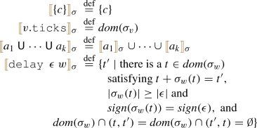
  A constant c defines the set of time instants that only contains c. The $\mathtt {ticks}$ of a stream variable defines the set of ticks that v is assigned in the valuation $\sigma$. The union $\mathrel {\textsf {U}}$ is interpreted as the union of sets of ticks. Finally, the operator $(\mathtt {delay}{}~~\epsilon ~w)$ defines the set of times $t+v$ such that there is an event (t, v) in w, with v of the same sign as $\epsilon$, and $|v| \ge |\epsilon |$; and there is no event between t and $t+v$. Notice that if the stream w produces an event whose value is either of a different sign than $\epsilon$, or is closer to zero than $\epsilon$, then it does not induce a time instant to be added to the set, but it still might prevent the previous value $t+v$ in w to be added to the set.

• Offset Expressions. Offset expressions calculate, given a time instant t, another time instant, or a symbol representing that the limits of the trace were surpassed. The semantics is given in Fig. 3. The interpretation of $\mathtt {t}$ is the current instant. For , the interpretation is the time of the event in the valuation of x (that is, $\sigma _x$) at the closest instant previous to the evaluation of at the current instant, or the value if there is no such event. For , the interpretation takes the evaluation of at the current instant, or the previous one at which $\sigma _x$ contains an event. The semantics of $\texttt {>>}$ and $\texttt {>}$ are dual to $\texttt {<<}$ and $\texttt {<}$ .

• Value Expressions. The semantics of the value expressions are given for an instant t:

  

  The interpretation of a stream access for x at e is the value of the stream $\sigma _x$ at the time t in case the evaluation of e is t and $\sigma _x$ is defined at t; otherwise it is or . The interpretation of a function is the corresponding interpreted function on the evaluation of the arguments, which includes as particular case the interpretation of constant d (as the value d). We rely on the type system to guarantee that the arguments have values of the right domain. The evaluation of $\mathtt {t}$ is the current value t. Similarly, the interpretation of offsets is the corresponding instants of time given by the evaluation of offset expression. Finally, the interpretation of $\texttt {-out}$ and is the values and . Note that includes the possibility that (1) the expression cannot be evaluated because the time instant given by is outside the boundaries of domain of the stream and (2) the expression is not defined because the stream does not tick at t. It is easy to see that the cases for are exhaustive because guarantees that is defined.

We are now ready to define evaluation models as follows.

Definition 2

(Evaluation model) Given a valuation $\sigma$ of variables $I\cup O$, the evaluation of the equations for stream $y\in O$ is the event sequence defined as follows:

An evaluation model is a valuation $\sigma$ such that for every $y\in O$: .

In other words, a candidate valuation $\sigma$ is an evaluation model if $\sigma$ satisfies all ticking equations and all value equations for all defined stream variables. Note that if an instant t is not in the domain of a stream s, then there is no d to comply with the definition and then $(t,d) \notin \sigma _s$.

The goal of a Striver specification is to define a monitor that intuitively should be a computable function from input streams into output streams. The following definition captures whether a specification indeed corresponds to such a function.

Definition 3

(Well-defined) A specification $\varphi$ is well-defined if for all $\sigma _I$, there is a unique $\sigma _O$, such that $\sigma _I\cup \sigma _O$ is an evaluation model of $\varphi$.

Specifications can be ill-defined. For example, the following specification

admits no evaluation model, and the following admits many evaluation models

3.4 Dependency graph

Definition 3 states that a specification $\varphi$ is well-defined if for every valuation of the input streams $\sigma _I$ there is a unique valuation of the output streams $\sigma _O$ that makes $(\sigma _I,\sigma _O)$ an evaluation model. Well-definedness is a semantic condition, which is not easy to check for a given specification (undecidable for expressive enough domains). Following [11, 28], we present here a syntactic condition, called well-formedness, that is easy to check on input specifications and guarantees that specifications are well-defined.

Given a set of streams Z, we define the subsets of Present, Past and Future offset expressions as the smallest subsets of offset expressions such that:

• $\mathtt {t}\in \textit{Present}$,

• if $e\in \textit{Future}$ and $x\in {}Z$, then

  • ,

  • ,

  • and

  • 

• if $e\in \textit{Present}$ and $x\in {}Z$, then

  • ,

  • ,

  • and

  • 

• if $e\in \textit{Past}$ and $x\in {}Z$, then

  • ,

  • ,

  • and

  • 

Note that $e\in \textit{Future}$ models whether e may be an instant in the future in some valuation. In other words, if $e\notin \textit{Future}$, then it is guaranteed that $\llbracket e\rrbracket _\sigma (t)$ cannot refer to the future of t in any valuation $\sigma$.

Definition 4

(Direct dependency) We say that y has a present direct dependency on x (and we write $x\xrightarrow {0}{}y$) if

• $x.\mathtt {ticks}$ appears in $\textit{C}_y$, or

• $\textit{V}_y$ contains some present expression $\tau _x\in \textit{Present}$.

We say that y has a past direct dependency on x (and write $x\xrightarrow {-}{}y$) if

• $\mathtt {delay}{}~\epsilon ~x$ appears in $\textit{C}_y$ and $\epsilon > 0$, or

• $\textit{V}_y$ contains some past expression $\tau _x\in \textit{Past}$.

We say that y has a future direct dependency on x (and write $x\xrightarrow {+}{}y$) if

• $\mathtt {delay}{}~\epsilon ~x$ appears in $\textit{C}_y$ and $\epsilon < 0$, or

• $\textit{V}_y$ contains some future expression $\tau _x\in \textit{Future}$.

In turn, dependencies allow creating a graph with three kinds of edges that represent future, past and present dependencies. This graph is easily computed from the specification and it has linear size in the size of the spec.

Definition 5

(Dependency graph) Given a specification $\varphi =\langle I,O,\textit{V},\textit{C}, \textit{T}\rangle$ the dependency graph is a directed graph $G_\varphi =(Z,E)$, where set of vertices is $Z = I \cup O$, and set of edges is $E : Z \times Z \times \{ \xrightarrow {0}, \xrightarrow {-}, \xrightarrow {+}\}$, where there is an edge $(x,y,t) \in E$ whenever $x \xrightarrow {t} y$ (for $t\in \{=,+,-\}$).

A path in the dependency graph is a past path if it contains at least one past dependency edge $\xrightarrow {-}$ and it does not contain any future dependency edge $\xrightarrow {+}$. A path in the dependency graph is a future path if it contains at least one future dependency edge $\xrightarrow {+}$ and does not contain any past dependency edge $\xrightarrow {-}$. Note that future paths model paths that necessarily refer to a future time instant, while past paths model paths that necessarily refer to a past instant. If a path is neither future nor past, then it may refer to the current instant. The condition of well-formedness restricts the different kinds of paths in circular dependencies of a given specification.

Definition 6

(Well-formed specifications) A specification $\varphi$ is well-formed if for every maximal strongly connected component (MSCC) M in its dependency graph, either every closed path in M is a past path or every closed path in M is a future path.

Closed paths are those paths whose initial and final vertices are the same. Closed paths in the dependency graph of a specification $\varphi$ capture dependencies between a stream and itself. Therefore the fact that all closed paths in a given MSCC are future or past guarantees that no circular dependency can refer to the current instant. In turn, this guarantees that there are no circularities in the information needed to compute the value of a stream at a given instant. The well-formedness condition is easy to check for a given specification and it implies that the dependency graph consists of a DAG of MSCCs, each of which is either future or past.

Theorem 1

Every well-formed Striver specification is well-defined.

Proof

Let $\varphi$ be a well-formed specification and consider an arbitrary valuation $\sigma _I$ of the input stream variables of the specification. By assumption, every stream in this input valuation has a finite number of events because they are non-Zeno and the temporal domain is restricted to have a minimum value $\bar{0}$ and a maximal value $\bar{1}$.

We reason by induction in a reverse topological order between the MSCCs, showing that for every MSCC M there is a single valuation of the stream variables in M assuming that all stream variables in lower MSCCs (we call these the inputs to M) have a single valuation. Also, assuming that the input valuations are non-Zeno, the output valuations are also non-Zeno.

Assume that M is a future MSCC (the other case is completely dual). We first define the following “quantum” duration for M as follows:

$$\begin{aligned} q \,{\mathop {=}\limits ^{\text {def}}}\,\textit{min}\{ -\epsilon \;\mid \; (\mathtt {delay}{}~\epsilon ~w)\in C_x \text { for any }x,w\in M\} \end{aligned}$$

For MSCCs that do not contain a delay, any constant time $q>0$ can be taken. The definition of quantum for past MSCCs is identical, except that $\epsilon$ is used for $-\epsilon$. It is easy to see that the existence of an element in an expression $\mathtt {delay}{}~\epsilon ~w$ at t only depends on $\sigma _w$ in the interval $[t+q, \bar{1} ]$ because the offset is at least q. We now divide the global duration of the streams $[\bar{0},\bar{1} ]$ into a sequence of $\lceil \frac{\bar{1}}{q}\rceil$ intervals of duration q:

$$\begin{aligned} {[}\bar{0},\bar{0} +q),[\bar{0} +q,\bar{0} +2q),\ldots ,[\bar{0} +nq,\bar{1} ] \end{aligned}$$

We use $I_i$ for the i-th interval in this sequence. We now reason by induction from $i=n$ down to 0 to show that there are only finitely many candidates $t\in I_i$ that can be a solution to $T_x$ for some $x\in M$. Take the first atomic expression in $T_x$ for $x\in M$. The case for $s.\mathtt {ticks}$ and $\mathtt {delay}{}~\epsilon ~s$ where $s\notin M$ can only generate a finite number of ticks in $I_i$ because $\sigma _s$ only has a finite number of ticks by assumption. The case for $\mathtt {delay}{}~\epsilon ~w$ where $w\in M$ can only generate as many ticks as $\sigma _w$ has in $\cup _{j>i} I_j$ because the offsets must be at least of q by the definition of q.

Finally, the constructs $w.\mathtt {ticks}$ and $\mathrel {\textsf {U}}$ do not generate new ticks except ticks already included in the previous cases. Finally, we show that for the finite number of time instants in an interval $I_i$, the finite number of ticking candidates $\{t_0<t_1< \ldots < t_k\}$ in the interval $I_i$ for $\llbracket T_x,V_x\rrbracket _{t_j}$ is completely determined for every $t_j\in \{t_0,\ldots ,t_k\}$. Note that every closed path in a future MSCC contains at least a future edge. Therefore, removing future edges, the MSCC M becomes a DAG. Evaluating in a reverse topological order < in this DAG guarantees that at time $t_j$ the values of the streams at $t_j$ necessary to compute the value of x at $t_j$ are known. A case inspection in the structure of $T_x$ and $V_x$ reveals that $\llbracket T_x,V_x\rrbracket _\sigma$ is completely determined by the events in $\sigma _s|_{[t_j,\bar{1} ]}$ if $s<x$, and in $\sigma _s|_{[t_{j+1},\bar{1} ]}$ otherwise. We then conclude that there is a unique solution for every $\sigma _x$ in the interval $I_i$, which has a finite number of events. Since there is a unique valuation for $\sigma _x|_{[t_j,\bar{1} ]}$ for every time instant $t_j$ in every interval $I_i$, we conclude that there is a unique solution for every $\sigma _x$ within $[\bar{0},\bar{1} ]$. $\square$

The proof above implies that for every well-formed specification, the input valuation determines uniquely a single valuation $\sigma _x$ for every stream x. Additionally, in order to determine the value of streams in future MSCCs one only needs to inspect the present and future of streams in the same MSCC, or values of streams in lower MSCCs. Dually, for past MSCCs only the past needs to be inspected. More importantly, the finiteness and acyclicity of the dependencies between events in the evaluation model allow us to reason by induction to prove that operational monitoring algorithms indeed compute the evaluation model.

4 Operational semantics

We show now the operational semantics of Striver. We first present in Sect. 4.1 a monitoring algorithm for the past fragment of Striver, this is, an algorithm to monitor Striver specifications whose dependency graph does not contain positive edges ($\xrightarrow {+}$). This algorithm allows to compute incrementally the output streams from the input streams, and its resources consumption is trace length independent. Then, in Sect. 4.2 we show a general algorithm for the full version of Striver, which includes also future operators.

4.1 Operational semantics for past specifications

The semantics of Striver specifications introduced in Sect. 3.3 are denotational in the sense that these semantics guarantee that for every input stream valuation there is exactly one output stream valuation, but does not provide a procedure to compute the output streams, let alone do it incrementally. We provide in this section an operational semantics that computes the output incrementally for the past fragment of Striver. Note that in the past fragment the dependency graph only contains $\xrightarrow {-}$ and $\xrightarrow {0}{}$ edges. We fix a past specification $\varphi$ with dependency graph G, and we let $G^=$ be its pruned dependency graph (obtained from G by removing $\xrightarrow {-}$ edges). We also fix < to be an arbitrary total order between stream variables that is a reverse topological order of $G^=$.

We first present a simple online monitoring algorithm that stores the full history computed so far for every output stream variable. Later, we will provide bounds on the portion of the history that needs to be remembered by the monitor, showing that only a bounded number of events needs to be recorded, and that this bound depends linearly on the size of the specification and not on the length of trace. The modified algorithm is a trace length-independent monitor for past Striver specifications.

The following auxiliary lemma captures sufficient information to determine the value of a given stream at a given time instant.

Lemma 1

Let y be an output stream variable of a specification $\varphi$, $\sigma$, $\sigma '$ be two evaluation models of $\varphi$, such that, for time instant t:

• (i) For every variable x, either

  $t' \notin \textit{dom}(\sigma _x)$ and $t' \notin \textit{dom}(\sigma '_x)$ or

  $\sigma _x(t')=\sigma '_x(t')$, for every $t'<t$, and

• (ii) For every variable x, such that $x\xrightarrow {\smash {0}}^*{}y$, either

  $t' \notin \textit{dom}(\sigma _x)$ and $t' \notin \textit{dom}(\sigma '_x)$ or

  $\sigma _x(t')=\sigma '_x(t')$, for every $t'\le {}t$.

Then, $\sigma _y(t)=\sigma '_y(t)$.

Proof

It is easy to see that if and only if , by structural induction on ticking expressions. The key observation is that only values in the conditions of the lemma are needed for the evaluation, which are assumed to be the same in $\sigma$ and $\sigma '$. Similarly, it is easy to see that because again the values needed are the same in $\sigma$ and $\sigma '$. $\square$

The online algorithm for the past fragment maintains the following state $(H,t_{q})$:

• History: H contains a finite event stream for each output stream variable. We use $H_y$ for the event stream prefix for stream variable y.

• Quiescence time: $t_{q}$ is the time up to which all output streams have been computed.

The monitor runs a main loop, which first calculates the next time $t_{q}$ that is relevant to the monitoring evaluation, and then computes all outputs up to time $t_{q}$. We will show that no event can exist in any stream in the interval between two consecutive quiescence time instants. We assume that at time t, the next event for every input stream is available to the monitor, even though knowing that there is no event up-to some $t<t'$ is sufficient.

The core observation that allows the design of our incremental algorithm follows from Lemma 1, which limits the information that is necessary to compute whether stream y at instant t contains some event (t, d) and the value d within the event. All this information is contained in H, so we write and to remark that only H is needed to compute and .

The main algorithm, PastMonitor, is shown in Algorithm 1. Lines 2 and 3 set the history and initial quiescence time. The main loop continues until no more events can be generated. Line 5 computes the next quiescence time, by taking the minimum instant after the last quiescence time at which some output stream may tick. A stream y “votes” (see Algorithm 2) for the next possible instant (in the future of the current quiescence time) at which its ticking equation $T_y$ can possibly contain a value. Consequently, no event can possibly be present between the current quiescence time and the lowest vote. Note that recursion at lines 27 and 29 terminates because the graph $G^=$ is acyclic. (Recall that the specification is well-formed.)

If the voted next quiescence time is $\infty$, it means that all streams have been completed, and thus, the algorithm ends. This behavior is reflected in line 6. If the voted next quiescence time is a time instant t, then the algorithm calculates the potential value of each stream at t in topological order < over $G^=$, so the information about the past required in Lemma 1 is contained in H. For every stream, if the calculated potential value is not , then the event is added to the history of the stream (in line 11) and emitted as an output of the monitor (in line 12).

Note that at every cycle, we need the next event on all input streams at a time instant greater than the current quiescence time. The algorithm will block until all such events occur. As a consequence, the input streams will be inspected and processed at different paces according to the global time. If an input stream s has been consumed completely, then the result of ${{\,\mathrm{{\textit{succ}}}\,}}_{>}(\sigma _s,t)$ will be $\infty$ at every succeeding cycle. Finally, note that ${\textit{latest}} (H_s)$ in line 23 returns the latest event in the past history of stream s (which is guaranteed to be non-empty due to the test in lines 19 and 20).

The following result shows that assuming that $\sigma _I$ is non-Zeno, the output is also non-Zeno. Hence, for every instant t, the algorithm eventually reaches a quiescence time $t_{q}$ greater than any given t in a finite number of executions of the main loop.

Lemma 2

PastMonitor generates non-Zeno output for a given non-Zeno input.

Proof

Note that events are generated in strictly increasing time for every stream, because the quiescence time $t_{q}$ decided in line 5 is greater than the current time. However, that does not imply non-Zenoness because some time domains (like the reals and the rationals) accept infinite sequences of increasing time stamps that do not pass a given instant t.

Now, we first show that if the output generated by the monitor is Zeno for time t (that is, there is no bound on the executions of the loop body that make $t_{q}>t$), then the execution is also Zeno for time $t-\epsilon$. The lemma then follows because by repeating the result $\lceil \frac{t}{\epsilon }\rceil$ times we will obtain that there is a Zeno execution that does not pass $t-\epsilon \frac{t}{\epsilon }=0$, but the second execution already passes 0.

Consider one such offending t. There must be an output stream variable x that votes infinitely many times in the infinite sequence of increasing quiescence times that never pass t. Let x be the lowest such stream variable in $(G^=,<)$. Consider the ticking expression for x. Since $\mathrel {\textsf {U}}$ collects the votes for its sub-expressions, it follows that some sub-expression votes for infinitely many quiescence times in the sequence. The sub-expression cannot be $s.\mathtt {ticks}$, because s would be lower than x in < (contracting that x is minimal). Hence, the sub-expression voting infinitely many times is of the form $(\mathtt {delay}{}~\epsilon ~s)$.

Then, all these votes are caused by different events in $H_s$ that are ticks of s that happened earlier than $t-\epsilon$. $\square$

We finally show that the output of PastMonitor is an evaluation model. We use $H^i_s(\sigma _I)$ for the history of events $H_s$ after the i-th execution of the loop body and $H^*_s(\sigma _I)$ for the sequence of events generated after a continuous execution of the monitor. Note that $H^*_s(\sigma _I)$ is a finite sequence of events if time is bounded by $\bar{1}$, or if all inputs have a finite number of events and no repetition is introduced in the specification using $\mathtt {delay}{}$. In this case, the vote is eventually $\infty$ and the monitoring algorithm halts. However, this algorithm can also be used (guaranteeing finite memory) for the continuous online evaluation ad infinitum for unbounded input events or the cyclic generation of events with $\mathtt {delay}{}$.

Theorem 2

Let $\sigma _I$ be an input event stream, and let $\sigma _O$ consist of $\sigma _x=H^*_x(\sigma _I)$ for every output stream x. Then, $(\sigma _I,\sigma _O)$ is an evaluation model of $\varphi$.

Proof

Let $\sigma$ be $(\sigma _I,\sigma _O)$. By Lemma 2, the sequence of quiescence times is a non-Zeno sequence. We show by induction on the votes of PastMonitor that for every quiescence time $t_{q}$, $\sigma$ is an evaluation model up to $t_{q}$, that is $H^*_x\vert _{t_{q}}=\llbracket T_x,V_x\rrbracket _\sigma \vert _{t_{q}}$.

Let $t_{q}^{\textit{prev}}$ be a quiescence time and let

$t_y=\textsc {vote}(H,y.\mathtt {ticks},t_{q}^{\textit{prev}})$.

We first show that for every output stream y, and for no $t'$ with $t_{q}^{\textit{prev}}<t'<t_y$, . This result follows by induction on <, by Lemma 1 which guarantees that only the past is necessary to evaluate , and by our assumption that $\sigma$ is an evaluation model up-to $t_{q}^{\textit{prev}}$. Now, let $t_{q}$ be the next quiescence time after $t_{q}^{\textit{prev}}$ chosen in line 5. We show, again by induction on <, that for every output stream variable y, $H_y$ contains an event $(t_{q},v)$ if and only if (which we showed above), and as computed in line 9. Hence, all events in $H_y$ satisfy that $(t_{q},v)\in \llbracket T_y,V_y\rrbracket _\sigma$ and all events $(t_{q},v)\in \llbracket T_y,V_y\rrbracket _\sigma$ are added to $H_y$ at quiescence time $t_{q}$. Since only quiescence times can satisfy , it follows that $\sigma$ is an evaluation model up-to $t_{q}$ if $\sigma$ is an evaluation model up-to $t_{q}^{\textit{prev}}$, as desired. Finally, since the set of quiescence times is non-Zeno, for every t there is a finite number n of executions of loop body after which $t_{q}^n\ge t$. Then, after n rounds $\sigma$ is guaranteed to be an evaluation model up to t. Since t is arbitrary, it follows that $\sigma$ is an evaluation model. $\square$

Putting together Theorem 2, and Lemmas 1 and 2, we obtain the following result.

Corollary 1

Let $\varphi$ be a well-formed specification, $\sigma _I$ a non-Zeno input stream and $H^*$ the result of PastMonitor. Then, $H^*$ is the only evaluation model for input $\sigma _I$, and $H^*$ is non-Zeno.

The uniqueness of the evaluation model for a well-formed specification is guaranteed by Theorem 1.

4.1.1 Trace length independent monitoring

The algorithm PastMonitor shown above computes incrementally the only possible evaluation model for a given input stream, but this naive algorithm stores the whole prefix $H_y$ for every output stream variable y. We show now a modification of the algorithm that is trace length independent, based on the notion of flat specification. A specification is flat if every occurrence of an offset expression is either of the form or . In other words, there can be no nested term of the form or or or . We first show that every specification can be transformed into a flat specification. The flattening applies incrementally the following steps to every nested term , where E is an arbitrary offset term:

• 1. introduce a fresh stream s with equations $T_s = y.\mathtt {ticks}$ and $V_s = x(E(\mathtt {t}))$

• 2. replace every occurrence of by .

Example 5

Consider a continuous integration process in software engineering, described using the following specification. The intended meaning of stream is to report those commits to a repository that fail the unit tests.

After applying the flattening process, the specification becomes:

Here, s stores the of the last commit at the point of a , which is precisely the information to report at the time of a commit. $\square$

Lemma 3

Let $\varphi$ be a specification. There is an equivalent flat specification $\varphi '$ that is linear in the size of $\varphi$.

Now, let $\varphi '$ be the flat specification obtained from $\varphi$ and let y be an output stream variable. Consider the cases for offset sub-expressions in the computation of in line 9 of PastMonitor:

• : the evaluation fetches the value $H_s$ at time t (if s ticks at t) or at the previous ticking time (if s does not tick at t).

• : the evaluation fetches the value $H_s$ at the previous ticking time of s.

In either case, only the last two elements of $H_s$ are needed. The similar argument can be made to compute $T_y$ because only the last event of s is needed for $(\mathtt {delay}{}~\epsilon ~s)$. Hence, to evaluate PastMonitor on flat specifications, the algorithm only needs to maintain the last two elements in the history for every output stream variable to compute the next value of every value and ticking equation.

Theorem 3

Every flat specification $\varphi$ can be monitored online with linear memory in the size of the specification and independently of the length of the trace. Moreover, every step can be computed in linear time on the size of $\varphi$.

Proof

We apply the flattening step until every output stream definition is flat. $\square$

4.2 Operational semantics for full Striver

We now present operational semantics of the full Striver language, including future and past references. As for the algorithm presented in Sect. 4.1, the new algorithm proceeds forward calculating the next event for each output stream. The main idea of this algorithm is to decouple the instant of this calculation for each individual stream. Before, there was a single quiescence time common to all streams, but the new algorithm proceeds with a potentially different time for each stream.

As we did for the past fragment, we show a simple algorithm focusing on simplicity instead of efficiency. However, for the general algorithm shown in this section, there are cases that force the algorithm to maintain an unbounded portion of the calculated history. This is unavoidable as the monitoring problem for future Striver not trace length independent in general. Some cases can be optimized though. For example, it is easy to see that using the operational semantics presented in this section, a specification whose dependency graph is a tree can be monitored in a trace length-independent manner if the monitor has the additional power of choosing the speed at which each of the input streams is processed. A shared node in the dependency graph means that the events in one stream (say s) influence another (say x) through different sub-expressions $e_1$ and $e_2$. It is possible that $e_1$ and $e_2$ need events from the common stream s that are arbitrarily far from each other, and between these events there may be an arbitrary number of intermediate events (which cannot be bound a priory) These intermediate events have to be buffered by the engine for their future use. It is work in progress to characterize other classes of specifications that can be monitored in a trace length independent manner, other than those whose dependency graph is a tree.

First, we define the type $\textit{Iterator}$ as $\textit{Id}\times \mathbb {T}$, whose values are pairs formed by a stream identifier and the timestamp of the last value calculated for the stream. This value corresponds to the time up to which the stream has been computed which essentially separates quiescence time for every stream. The constants $\textsf {-out}$ and $\textsf {+out}$ are used to represent out of the bounds (initial and final, resp.). All stream histories are initialized as empty lists. Given an iterator $\textit{it}=(s,t)$, we use $\textit{it}.\textit{stream}$ for the stream s and $\textit{it}.\textit{time}$ for the time t. Given an event $e=(t,d)$, we use $e.\textit{time}$ for the time t of the event and $e.\textit{val}$ for the value d.

Monitor. We initialize an iterator for every stream and save it in a map called $\textit{outIters}$. The monitoring algorithm monitor, shown in Algorithm 3, keeps calculating further events for all streams in $\textit{outIters}$. For each iterator, the algorithm computes the next value, progressing in time. When an event is computed, this is emitted to the environment as a monitor observation. Therefore, for every stream, the events are generated in increasing time order (note that different streams need not emit the events in increasing order with respect to each other). If the retrieved value for s is $\textsf {+out}$, this means that $\sigma _s$ will not contain any more values and the iterator of s is removed from $\textit{outIters}$.

Iterator functions. Iterators are equipped with the following methods, shown in Algorithm 4. The function next returns the next event strictly in the future of the time in the state of the iterator. Such event can be a progress event, which means that there are no actual values up to the computed time t, and encodes the processing of the stream up to t in cases where there is no event at t. The simple naive implementation of next shown here loops through the elements in the History of the stream, until it finds the first event with a timestamp greater than the iterator’s time, and returns the updated iterator, along with the computed event. This event can be already present in the history because the iterators for other streams could have triggered progress in the computation of the history of s. If such an event is not found in the History, the function calls solveNext for the computation of the next event in the valuation of stream s. The event computed is added to the History of the stream, removing the last value stored if it was a $\textsf {notick}$ (that is, a progress event), which guarantees that histories can only have a $\textsf {notick}$ as the last event. In other words, progress events are only used to encode the precise quiescence time of the stream. The calculated actual event is returned along with the new state of the iterator. The function peekPrev retrieves the previous event before a certain t, or $\textsf {-out}$ if t is the timestamp of the first event in the trace. As a precondition, there has to be an event with timestamp t in the History (which is in turn always guaranteed in the algorithm).

Spec execution. The calculation of the next value for a given stream is performed by calling solveNext, shown in Algorithm 5. If the event history $H_s$ is empty, this computation will call calculateNextTime with $-\infty$ as the last timestamp. Otherwise, the computation will use the timestamp of the last event in the history of s. If the event returned by calculateNextTime is a progress event (indicated by a $\textsf {notick}$ value), it means that the ticking expression returned progress but no actual event, and this progress event is returned. This also covers the case where the returned event is $\textsf {+out}$. If a real tick candidate is returned by calculateNextTime (indicated by a () value, read as unit), this is used to compute the value that corresponds to the denotational semantics of the specification. Note that these semantics may invoke prev, prevEq, succ or succEq according to the expression of $V_s$, potentially triggering the progress of other stream iterators. An event with the timestamp of the tick and the computed value is returned.

Tick calculation. For the calculation of the next potential tick after t for a $\mathtt {delay}$ of a stream s with positive delays (a stream with time values $v \ge \epsilon >0$), the procedure calculateNextTime iterates until it finds an event with a timestamp greater than t. This procedure is shown in Algorithm 6. If the event found is the first event (that is, if $\textsc {peekPrev}$ returns -out), then we can conclude that no tick happens up to the time of that event, and this is all we can conclude. If the event found is not the first event, the procedure considers the previous event, and adds its timestamp and its value. If the result is not in the time domain, this is, it is greater than $\bar{1}$, then we output $\textsf {+out}$. Otherwise, the algorithm checks whether the last event is overridden by the following event. If it is not overridden, the value generated was greater or equal to $\epsilon$, and the corresponding time computed is greater than the argument t, then we output the time of the event along with the unit value. This case corresponds to the $\mathtt {delay}$ producing an actual tick. If it was overridden, it was lower than $\epsilon$ or it has already been output (indicated by the fact that the value is lower or equal to t), then no tick will happen until the time of the next event.

If the expression is a negative $\mathtt {delay}$ , then we find the next non-progress event in the stream s. If we reach the end of the stream, we output $\textsf {+out}$. Otherwise, we add the timestamp and value of the event and check whether the result is greater than t, in the time domain (this is greater or equal to $\bar{0}$), and the value was lower or equal to $\epsilon$. If the condition is met, the time of the corresponding event is returned with the unit value. If it is not, then no event will be produced until the timestamp of the next event.

For a constant expression, if the constant is greater than t, then it is returned with the unit value. Otherwise, the procedure returns $\textsf {+out}$.

For a $s.\mathtt {ticks}$ expression, the procedure iterates over s until it finds the first event with a timestamp greater than t and returns its timestamp along with the unit value.

Finally, for U, calculateNextTime finds the lowest timestamp greater than t for each argument stream and then proceeds in the following way. If the timestamps are the same, and the two values are $\textsf {notick}$, then a $\textsf {notick}$ at the timestamp is produced. If the timestamps are the same, but one of the two values is not $\textsf {notick}$, then a unit value at the timestamp is produced. Otherwise, the event whose timestamp is the lowest is returned.

Stream access methods. We finally describe the implementation of prev, prevEq, succ and succEq that implement ${{\,\mathrm{{\textit{prev}}}\,}}_{<}$, ${{\,\mathrm{{\textit{prev}}}\,}}_{\le }$, ${{\,\mathrm{{\textit{succ}}}\,}}_{>}$and ${{\,\mathrm{{\textit{succ}}}\,}}_{\ge }$from the denotational semantics. This is shown in Algorithm 7.

• To calculate ${{\,\mathrm{{\textit{prev}}}\,}}_{<}$, prev iterates until if finds the first event with a timestamp greater than t on s, and returns the event immediately preceding.

• To calculate ${{\,\mathrm{{\textit{prev}}}\,}}_{\le }$, prevEq iterates until it finds the first event with a timestamp greater or equal to t on s. If such event has timestamp t and it is not a progress event, it is returned. Otherwise, prevEq behaves just like prev.

• To calculate ${{\,\mathrm{{\textit{succ}}}\,}}_{>}$, succ iterates until it finds the first non-progress event with a timestamp greater than t on s, or $\textsf {+out}$, and returns this event.

• To calculate ${{\,\mathrm{{\textit{succ}}}\,}}_{\ge }$, succEq iterates until it finds the first non-progress event that has a timestamp greater or equal to t on s, or $\textsf {+out}$, and returns it.

The correctness of the algorithm means that the operational semantics implemented by the algorithm outputs all events in the evaluation model for every output stream, and only those events. This is easily shown by induction on the well-formed graph of the finite set of events in the unique evaluation model, guaranteed to exist and be unique by Theorem 1.

5 Comparison with other formalisms

5.1 Comparison with TeSSLa

We compare in this section Striver with the TeSSLa specification language [16]. Even though TeSSLa is defined both for event streams and piece-wise constant signals, event streams and piece-wise constant signals can be easily converted into each other (see, e.g., [22]). We show in this section that TeSSLa can be translated into Striver under the assumptions described below, where the main difficulty is related to the delay operator and the possibility of generating Zeno outputs. Essentially, the decisions in the design of Striver presented in the previous sections guarantee that all outputs are non-Zeno (if all inputs are), while on the other hand, TeSSLa accepts specifications that generate non-Zeno outputs. We modify the delay operator in this section to increase the expressivity of Striver here to be able to cope with these additional specifications.

The design principle of TeSSLa is not to handle explicit time and offsets but instead to offer stream transformers that can be combined to build specifications. A TeSSLa specification consists of a collection of stream variables $Z=I\cup O$ and set of recursive equations of the form $y{:}{=}e$ with $y\in O$ using the following operators:

$$\begin{aligned} \begin{array}{rcl} e &{}{:}{:}=&{} \mathbf{nil} \big |\mathbf{unit} \big |x \big |\mathbf{lift} (f)(e,\ldots , e) \big |\mathbf{time} (e) \big |\\ &{}&{} \mathbf{last} (e, e) \big |\mathbf{delay} (e,e) \end{array} \end{aligned}$$

where x is a stream variable. The meaning of nil is the empty stream that contains no events. The operator unit models the unique stream of type unit that only contains a single event, at time 0. The terminal x allows referring to other streams in the specification. The operators lift, time, last and delay are stream transformers, that is, they return streams from other streams. The operator time returns a stream that contains the same ticks as the stream passed, except that the values are the instants at which the events occur. The operator lift allows using functions from data domains by applying them to the current or previous values of the argument streams. The operator $\mathbf{last} (v,r)$ takes two streams, v for values and r for triggers; last returns a stream at the ticking times of r with the previous value of v. Finally, $\mathbf{delay} (d,r)$ takes two streams: a delay stream d and a reset stream r. The output is a stream of type unit that has an event at time t when d has an event $(t-v,v)$, there is no event in r in the time interval $(t-v,t)$, and either there was no tick pending or there is an event in r at instant $t-v$ as well.

We now present a translation from TeSSLa specifications that are non-Zeno to Striver. The set of stream variables is the same, and each equation is translated independently. To simplify the translation we assume that the TeSSLa specification is flat, that is, all arguments of all operators are stream variables. Every specification can be easily flattened by introducing extra variables.

• nil: the stream $x {:}{=} nil$ is translated into:

  

• unit: the stream $x{:}{=}\mathbf{unit}$ is defined as:

  

• lift: the stream $x {:}{=} \mathbf{lift} (f)(s_0,\ldots ,s_n)$, where B is the co-domain of f, is translated into:

  

• time: the stream $x {:}{=} \mathbf{time} (s)$ is translated into:

  

• last: the stream $x {:}{=} \mathbf{last} (v,r)$, where v is a stream of type A is defined as:

  

The translation of TeSSLa ’s $\mathtt {delay}$ operator is more cumbersome as it allows the possibility of output event streams with diverging (Zeno) time sequences. Since both Striver and TeSSLa assume that inputs are non-Zeno, the only possibility to generate a sequence of Zeno time-stamps is by the $\mathtt {delay}$ operator generating ticks that are closer and closer. As defined in [16], TeSSLa still allows diverging outputs and classifies as legal those executions that do not diverge. For those specifications and inputs for which the TeSSLa operational semantics diverge the denotational and operational semantics of TeSSLa disagree. A design principle of Striver is to guarantee non-Zeno outputs, which was achieved in Sect. 3 by forcing the time of all delays to be larger than a constant $\epsilon$ (which can be arbitrarily small). Hence, since there are non-Zeno sequences in which the $\mathtt {delay}$ generates arbitrarily close events, the $\mathtt {delay}$ operator from Sect. 3 is not sufficient to translate TeSSLa to Striver, at least in an inductive way.

To capture all legal TeSSLa specifications, we introduce now a modified delay operator $\mathtt {delay}'{}~sgn~f~w$, where $\textit{sgn}$ is one of $\{\textit{pos},\textit{neg}\}$, f is a function with type $\mathbb {T} \rightarrow \textit{Bool}$ and w is a stream of type T as before. The intended meaning of f is to tell the delay operator whether to ignore or accept a given event. The semantics are:

We require that f be non-divergent for valuation candidate $\sigma$, that is, that the set of ticks is non Zeno. We can mimic the original semantics of Striver ’s $\mathtt {delay}$ by choosing $f(v) = |v| \ge |\epsilon |$, which is Zeno-convergent for any valuation. The function f serves as an oracle for delay to accept candidate ticks. The introduction of f imposes an obligation to the writer of the specification, who is now in charge of guaranteeing that f meets the requirement of preventing divergence. If this precondition is not met, then the denotational semantics of the Striver specification is undefined for such an offending trace, and the operational semantics will simply keep producing an ever close set of ticks. If the precondition is met, then the operational and denotational semantics will coincide. Note that this is not really a big practical limitation as a legal f can, for example, let a large number of events be generated and reset the counter if a certain $\epsilon$ has been passed since the first event.

With this modified $\mathtt {delay}$’ operator, we can define the translation of TeSSLa $\mathtt {delay}$ as follows:

• delay: the stream $x {:}{=} \mathbf{delay} (d,r)$ is translated into:

  

The choice of $f(v) = true$ as the argument for $\mathtt {delay}$ allows capturing the semantics of TeSSLa and guarantees that if a given TeSSLa specification is legal (generates non Zeno outputs for every input), then f is convergent for all inputs.

In [22], the authors present a non-blocking engine for a subset of TeSSLa, which can anticipate the computation of some streams even if not all the input streams have events. The operational semantics presented in Sect. 4.1 are kept simple for the sake of explanation, but it can be extended to mimic the asynchronous algorithm in [22] to evaluate and increment iterators independently, and block an iterator only when some of its necessary values is not present.

Theorem 4

The semantics of a legal TeSSLa specification $\varphi$ and the Striver specification $\varphi '$ resulting from following the shown translation over $\varphi$ are equal over any valid input.

Proof

(sketch) An easy induction on the structure of TeSSLa expressions allows proving that the resulting Striver specification obtained is equivalent. We sketch a proof for the case of $\mathbf{delay}$. The output stream x generates the unit value after the last alarm set by $x\_aux$, with a new value on $x\_aux$ overriding the pending alarm. The auxiliary stream $x\_aux$ behaves as follows: If stream d is generating an event, then $x\_aux$ decides whether it will emit the value or ignore it. If the reset stream is also generating a value, the delay is emitted. Alternatively, if the last alarm set by $x\_aux$ has already gone off (or if no alarm was ever set), then the delay is emitted. If there was a pending alarm and the reset stream is not generating a value, the delay is ignored, and $x\_aux$ produces a value. If instead the delay stream d is not producing a value (and thus, the reset stream r is), then we cancel any pending alarm by emitting a 0. $\square$

5.2 Comparison with signal temporal logic

We now show how Striver also subsumes the signal temporal logic (STL) [23, 24]. To do so, we extend the core Striver language with new constructors to allow the definition of properties over sliding windows without the need to introduce container-types in a given data theory. First, we introduce the notion of carried values which essentially allow tagging the timestamp at which a stream ticks with values from the ticking sub-expression that actually causes the tick. By itself, this extension does not add expressive power to the language, and could be expressed using the instruments presented in Sect. 3. The second extension introduces shift, which allows moving the ticks of another stream by a positive or negative constant. Together with the carried values, shift allows defining a shift stream transformer and truly sliding windows. In detail, we extend the Striver language with two new capabilities:

• 1. Carried values: Every time a value expression is computed at an instant t, it is because t belongs to its associated ticking expression, which in turn can be caused by other streams, by a constant or by a delay.

  The idea of the carried value is to give a way to access the values of the ticking streams from the value expressions. To achieve this, we enrich the evaluation context of the value expressions with a new language construct whose value is a tuple containing the values of the members in the ticking expression that induced the tick. We indicate the type of the carried value in the tick expression of the stream. In particular, if the n-th source of ticks is not producing a value at the time of evaluation, then the n-th element of is .

• 2. Shift: The constructor shift extends ticking expressions allowing to shift a stream by a constant duration.

  Together with carried values, we can trivially shift a stream by a given as follows:

  

  Note that the carried value allows fetching the value of s at a different time (after the delay ), which otherwise would require calculating the time instant and allow accessing values of streams at arbitrary times. Such a feature would increase the complexity of monitoring algorithms and typically requires preserving the whole trace of every stream.

We show how the addition of these constructors affects the syntax:

• Ticking Expressions: We add the $\mathtt {shift}$ operator to the ticking expressions.

  $$\begin{aligned} \begin{array}{lcl} \alpha &{}{:}{:}=&{} \alpha ' \big |\alpha ' \mathrel {\textsf {U}}\cdots \mathrel {\textsf {U}}\alpha ' \\ \alpha ' &{}{:}{:}=&{} \mathtt {\{} c \mathtt {\}} \big |v.\mathtt {ticks}\big |\mathtt {delay}{}~\epsilon ~w \big |\mathtt {shift}~c~v \end{array} \end{aligned}$$

  (1)

• Offset Expressions: Offset expressions are not affected by these extensions.

• Value Expressions: We add the constructor to access the carried values.

  

  (2)

  The additional expression $\mathtt {cv}$ represents the value carried by the ticking expression.

The idea is that the ticking expressions calculate not only a set of tick instants, but also a value associated with every potential tick instant. For the ticking expression $v.\mathtt {ticks}$, the associated value at instant t is $\sigma _v(t)$. For the ticking expression c, the associated value for each instant t is () (the unit value). For the ticking expression $\mathtt {delay}{}~\epsilon ~w$, the associated value for instant t is the value of w that made t become a tick instant. For the ticking expression $\mathtt {shift}~c~v$, the associated value for each instant t is $\sigma _v(t-c)$. Finally, for the ticking expression $e_0 \mathrel {\textsf {U}}\cdots \mathrel {\textsf {U}}e_k$, the associated value for each instant t is a k-tuple where each element $i = 1,\cdots ,k$ is the value carried by the expression $e_i$ if t is in the tick expression $e_i$, and otherwise.

This value carried by the tick expression can be accessed from the value expression with the new constructor $\mathtt {cv}$.

Note that if the tick expression does not have a $\mathtt {shift}$ expression, we can calculate the carried value using the original value operators using the construct isticking(r) and r( t) over every non-delayed tick expression of the form $r.\mathtt {ticks}$, and calculating with ${\texttt {r(<t)}}$ over every $\mathtt {delay}{}~\epsilon ~r$ tick expression.

We are now ready to show that Striver with these extensions subsumes signal temporal logic (STL) [23, 24]—when interpreted over piecewise-constant signals. Piecewise-constant signals are signals that only change value in finitely many points in every given interval and remain constant between two points of value change. The syntax of STL is

$$\begin{aligned} \varphi&{:}{:}= \textit{true} \big |\mu _f \big |\lnot \varphi \big |\varphi \mathrel {\vee }\varphi \big |\varphi \mathbin {\mathcal {U}}_{[a,b]}\varphi \end{aligned}$$

where f is a function from $\mathbb {R}^n$ to $\mathbb {R}$, and a and b belong to the temporal domain. The satisfaction relation is defined over a sequence x of real valued signals and a time-point t as follows.

Event streams have an alternative interpretation as piecewise-constant signals, where the signal changes at the points at which events are produced. A translation of STL into Striver like the one shown in this section enables the encoding of quantitative semantics of STL by enriching the data types of expressions and verdicts. We show here how to check STL Boolean properties by translating them to Striver specifications. The specification is constructed recursively over $\varphi$:

• True: We translate true as the stream tr as follows:

  

• Function sampling $\mu _f$:. We assume that the input signal is input D x and define the Boolean output signal mu_f as follows:

  

• Negation: Given the Boolean stream x for $\varphi$, we define the stream neg_x for $\lnot \varphi$ as follows:

  

• Disjunction: Given the Boolean streams x and y, for $\varphi _1$ and $\varphi _2$ (resp), we define the stream x_or_y for $(\varphi _1 \mathrel {\vee }\varphi _2)$ as follows:

  

• Until: Given Boolean streams x and y for $\varphi _1$ and $\varphi _2$ (resp), and given a and b we define the stream x_U_y for $(\varphi _1 \mathbin {\mathcal {U}}_{[a,b]} \varphi _2)$ as follows:

  

  Essentially, the intermediate stream shift_y_a defines a shift of y by exactly a time units, and then shift_yT_a filters out the events with value false and keeps occurrences of value true only. Hence, the time and value of the next event in shift_yT_a at any instant t correspond to the next time y becomes true after $t+a$. The expression min_y contains the earliest time at which y becomes true (considering the possibility of t itself if y is already true). Similarly, min_xF contains the earliest time at which x becomes false (considering the possibility of t itself if x is already false). With these auxiliary definitions, the value expression of x_U_y simply checks that y becomes true within [a, b] and that x is true from t up-to that point.

  The tick expression of the stream indicates the times at which its value can change, namely when a y event enters or leaves the sliding window defined by $[t+a, t+b]$, or when a x event enters or leaves the sliding window defined by $[t, t+b]$.

We use the constant infty to represent a value that is greater than any value of $\mathbb {T}$. The translation presented is bottom-up and simple, but it does not exploit the fact that, if b is not $\infty$, only a bounded future must be explored. As it is, the translation of until is a future specification. We extend now the language with bounded offset operators by redefining $\tau$-expressions as follows:

The semantics of the newly added operators is as follows: Considering ,

• If , then . Otherwise, behaves as at t.

• If , then . Otherwise, behaves as at t.

• If , then . Otherwise, behaves as at t.

• If , then . Otherwise, behaves as at t.

Mathematically, the semantics of is the following:

The semantics of the other operators are analogous. Even though these expressions do not enhance the expressive power of Striver, they enable the monitoring engine to stop seeking a value if the time progress grows beyond a bound. With this information, the engine can optimize the execution and even guarantee trace length independence assuming that the event rate is bounded. An empirical study on how using bounded operators affects the resource performance is included in Sect. 6. We can now use the operator to define a more efficient version of STL’s Until:

At instant t, the implementation will be keeping the events in y in the range $[t+a, t+b]$ and the events in x in the range $[t, t+b]$.

6 Empirical evaluation

In this section, we report on an empirical evaluation of Striver. We conduct two sets of experiments: one for the past fragment of Striver, that is guaranteed to run in bounded resources, and the other for the full version of Striver, including the extension shown in Sect. 5.2. All experiments were executed on a virtual machine running on an Intel Xeon at 3GHz with 32GB of RAM.

Fig. 4

Empirical evaluation of the past fragment of Striver

6.1 Past Striver

The empirical evaluation of past Striver is based on an implementation written in the Go programming language³ which is the core element of the Elastest Monitoring Service.⁴ We run experiments to measure the memory usage and time per event for two collections of specifications:

• The first collection generalizes Example 2 computing the stocks of p independent products. These specifications contain a number of streams proportional to p, where each defining equation is of constant size. Even though each output stream in the specification could be monitored in parallel, our engine is completely sequential.

  

• The second collection computes the average of the last k sales of a fixed product, via streams that tick at the selling instants and compute the sum of the last k sales. The resulting specifications have depth proportional to k.

  

We instantiate k and p from 10 to 500 and run each resulting specification with a set of generated input traces. We measure the average memory usage (using the OS) and the number of events processed per second.

In the first experiment, we run the synthesized monitors with traces of varying length (shown in the top two plots in Fig. 4). The results illustrate that the memory needed to monitor each specification is independent of the length of the trace. (The curves are roughly constant.) Also, the throughput of events processed is independent of the length of the trace and is a constant in the thousands of events per second in each experiment. In the second experiment, we fix a trace of 1 million events and run the specifications with k and p ranging from 250 to 550. The results (lower diagrams) indicate that the memory needed to monitor stock_p is independent of the number of products while the memory needed to monitor each avg_k specification grows linearly with k. Recall that theoretically all specifications can be monitored with memory linearly on the size of the specification.

Fig. 5

Empirical evaluation of the fully fledged version of Striver

6.2 Full Striver

We report an empirical evaluation of a prototype sequential Striver implementation, written in the Java programming language.⁵ For this set of experiments we consider a simple STL specification of a moving vehicle. The speed of the vehicle is an input stream of type . The property to specify is: “Whenever the vehicle is moving too fast, it must decelerate continuously until it reaches a safe speed within 5 s.” We say that the vehicle is moving too fast if its speed is greater than 1, and we define a safe speed as a speed under 0.8. We can write this property in STL as follows:

Note that this specification requires a Boolean input signal decel that indicates whether the vehicle is decelerating. We translate this property into Striver using the following specification, where is obtained by translating the Until operator as shown in Sect. 5.2.

Using Striver we measure the deceleration with the signal comparing its value at the current instant with the next value, and thus, there is no need of an extra input signal.

The input data, shown in Fig. 5a, c, are generated pseudo-randomly. Figure 5a shows an input illustrating under the graph (in green) the regions where $\varphi$ holds. Also, at the bottom we show the regions where the speed is too high, but where the car decelerates continuously until reaching a safe speed, within 5 time units. Fig. 5c shows a much longer input signal.

We translated the specification using bounded future operators and showed that the memory consumption of the monitor remains constant over the trace length. However, the memory requirement correlates linearly with the size of the window and with the input event rate, as can be seen in Fig. 5b.

On the other hand, if we use a Striver specification with unbounded future operators, then the memory requirement depends on the input signal and is no longer solely determined by the window size and input event rate. The memory usage of the different runs can be seen in Fig. 5d. In the Striver specification with unbounded future accesses, the Until expression needs to retrieve at a given time, the next instant at which the vehicle decelerates and also the next instant at which its speed is safe. If one of these instants is far in the future, the monitor engine needs to consume and store all the input up to that point. This causes a rapid increase in the memory consumption and is completely dependent on the shape of the input signal, which is in principle arbitrary. Once the relevant instants are found, the input signal is consumed up to that point, which causes a rapid decrease in memory consumption. As a result of this, we observe that memory usage presents peaks during the execution. The green curve in Fig. 5d represents the memory consumption of a run with the original safe speed, of 0.8. We can see that usually this value is reached quickly and keeps the memory below the maximum value, which was set at 1GB.

In the blue run, we modified the safe speed to $-1600$. This value requires more time to find the relevant time instants, resulting in higher peaks of memory usage, that go down at approximately time instant 40. From that point on, the speed of the car never comes back down to a value as low as $-1600$, and thus, the memory consumption reaches the maximum memory.

The red curve represents the memory consumption of a run with a safe speed of $-1750$. Since this value is never reached, or it is reached too far away in the input trace, the memory consumption goes up continuously well beyond the maximum memory threshold (without producing an output), and eventually the program crashes with a java.lang.OutOfMemoryError. Note how a small variation in the input data yields very different memory consumption curves for unbounded future specifications.

7 Final discussion and conclusion

We have introduced Striver, a stream runtime verification specification language for timed event streams, equipped with explicit time. We have presented a trace length-independent online monitoring algorithm for the past fragment, and we show empirically that it behaves as expected in terms of the bounds of resources. We have also presented an online monitoring algorithm for the full version of the language, and we show how its future fragment needs not be trace length independent. We have shown how to translate specifications in other specification languages, such as TeSSLa and STL, to Striver and we showed empirically that the memory requirement to monitor an STL specification is bounded by the ratio between input rate and the size of the intervals in the usage of Until operators.

Unbounded time domains. The semantics of Striver introduced in Sect. 3.3 requires temporal domains to have both a minimal element $\bar{0}$ and a maximal element $\bar{1}$ for all specifications to be well-defined in the general case. We describe here how to relax these requirements. The boundaries in the time domain are necessary for two reasons:

• First, to provide a base case for recursion, which is required by closed paths in the dependency graph. A negative cycle imposes the need for a $\bar{0}$, while a positive cycle imposes the need for a $\bar{1}$. For example, consider the following specification:

  

  There must be a value for s at 5, but if r produces infinitely many events, it is not possible to find an integer that satisfies the value equation of s.

• Second, to prevent faulty references to the occurrences of functions ${{\,\mathrm{{\textit{prev}}}\,}}_{<}$, ${{\,\mathrm{{\textit{prev}}}\,}}_{\le }$, ${{\,\mathrm{{\textit{succ}}}\,}}_{>}$ and ${{\,\mathrm{{\textit{succ}}}\,}}_{\ge }$, in the semantics of $\tau$ expressions. An expression or that uses an expression e whose value could be (for example ) imposes the need for a $\bar{1}$, while a or using an expression e whose value could be imposes the need for a $\bar{0}$. For example, consider the following specification:

  

  The stream s at 0 is trying to fetch the last value of r, which may not exist if r produces infinitely many events.

If we are dealing with a specification whose dependency graph does not have positive cycles, and there are no expressions or where the semantics of e could be , then there is no need to impose the presence of a $\bar{1}$ in the time domain. For example, this is the case when one uses only past expressions. Dually, if we are dealing with a specification whose dependency graph does not have negative cycles, and there are no expressions or where the semantics of e could be , then there is no need to impose the presence of a $\bar{0}$ in the time domain.

The operational semantics of the past-only fragment of Striver presented in Sect. 4.1 always converges to the correct evaluation model if the specification is well-defined. On the other hand, the operational semantics of the full language presented in Sect. 4.2 may diverge for well-defined specifications which do not contain positive cycles, do not define a $\bar{1}$, but use unbounded future accesses or negative delays. For example, the following specification is well-defined:

The stream generates a every 10 time units starting at 0, and the streams and have no events, something that can be easily deduced from their types. A smart compiler could realize that and have no events from their types or checking that the value expression of is , but an immediate application of the operational semantics algorithm will diverge trying to calculate the value of the stream at time 0. The main reason is that a future access (like ) requires to compute the next ticking instant of . Even though this is a single offset, this instant may be arbitrarily far in the future, or not even exist. Therefore, in a model of time where the future is unbounded, this computation may not terminate.

Language duality. There exists a duality between the past and the future operators of Striver, which can be exploited to offline monitor any specification using the online algorithm presented in Sect. 4.1 and following the idea of multiple passes used in Lola  [11, 28]. We start from a well-formed specification and partition its dependency graph into maximal strongly connected components (MSCC). Since the specification is well-formed, each of the MSCCs either has only positive cycles, or have only negative cycles. MSCCs with negative cycles will be computed from the beginning of the trace forwards. MSCCs with positive cycles will be computed from the end of the trace backwards. Every pass will store the output streams of the MSCCs being calculated in a local file storage. The dependency graph of MSCCs is actually a DAG, and the order of evaluation is a reverse topological order using the order induced by the dependencies. Independent MSCCs can be computed in parallel. If the specification does not contain both positive and negative cycles, then the whole specification can be computed using only one pass. The lack of cycles of any kind implies that well-definedness is not dependent on boundaries over the time domain, and that the direction of the computation can be freely chosen by the algorithm. In particular, the STL translation of a property yields a dependency graph with no cycles and thus can be computed both forward or backwards as desired.

Future work. Future work includes the extension of the language with parametrization, (like in quantified event automata (QEA) [29], MFOTL [30] and Lola2.0 [31]), to dynamically instantiate monitors for observed data items. We also plan to study offline evaluation algorithms, and algorithms that tolerate deviations in the time-stamps and asynchronous arrival of events from the different input streams, computing the values of the output streams as soon as the necessary data are available.

References

Havelund, K., Goldberg, A.: Verify your runs. In: Proceedings of VSTTE’05, LNCS 4171, pp. 374–383. Springer, Berlin (2005)
Leucker, M., Schallhart, C.: A brief account of runtime verification. J. Log. Algebraic Program. 78(5), 293–303 (2009)
Lectures on Runtime Verification-Introductory and Advanced Topics: Volume 10457 of LNCS. Springer (2018)
Havelund, K., Roşu, G.: Synthesizing monitors for safety properties. In: Proceedings of TACAS’02, LNCS 2280, pp. 342–356. Springer, Berlin (2002)
Eisner, C., Fisman, D., Havlicek, J., Lustig, Y., McIsaac, A., Van Campenhout, D.: Reasoning with temporal logic on truncated paths. In: Proceedings of CAV’03, Volume 2725 of LNCS 2725, pp. 27–39. Springer, Berlin (2003)
Bauer, A., Leucker, M., Schallhart, C.: Runtime verification for LTL and TLTL. ACM Trans. Soft. Eng. Methods 20(4), 14 (2011)
Sen, K., Roşu, G.: Generating optimal monitors for extended regular expressions. ENTCS 89(2), 226–245 (2003)
Asarin, E., Caspi, P., Maler, O.: Timed regular expressions. J. ACM 49(2), 172–206 (2002)
Barringer, H., Goldberg, A., Havelund, K., Sen, K.: Rule-based runtime verification. In: Proceedings of VMCAI’04, LNCS 2937, pp. 44–57. Springer, Berlin (2004)
Roşu, G., Havelund, K.: Rewriting-based techniques for runtime verification. Autom. Softw. Eng. 12(2), 151–197 (2005)
D’Angelo, B., Sankaranarayanan, S., Sánchez, C., Robinson, W., Finkbeiner, B., Sipma, H.B., Mehrotra, S., Manna, Z.: LOLA: runtime monitoring of synchronous systems. In: Proceedings of TIME’05, pp. 166–174. IEEE, New York (2005)
Pike, L., Goodloe, A., Morisset, R., Niller, S.: Copilot: a hard real-time runtime monitor. In: Proceedings of RV’10, LNCS 6418. Springer, Berlin (2010)
Goodloe, A.E., Pike, L.: Monitoring distributed real-time systems: a survey and future directions. Technical Report, NASA Langley Research Center (2010)
Bozelli, L., Sánchez, C.: Foundations of Boolean stream runtime verification. In: Proceedings of RV’14, Volume 8734 of LNCS, pp. 64–79. Springer, Berlin (2014)
Pnueli, A., Zaks, A.: PSL model checking and run-time verification via testers. In: Proceedings of FM’06, LNCS 4085, pp. 573–586. Springer, Berlin (2006)
Convent, L., Hungerecker, S., Leucker, M., Scheffel, T., Schmitz, M., Thoma, D.: TeSSLa: temporal stream-based specification language. In: Proceedings of the 21st. Brazilian Symposium on Formal Methods (SBMF’18), LNCS. Springer, Berlin (2018)
Faymonville, P., Finkbeiner, B., Schwenger, M., Torfah, H.: Real-time stream-based monitoring. CoRR. arXiv:1711.03829 (2017)
Cristian, F., Fetzer, C.: The timed asynchronous distributed system model. IEEE Trans. Parallel Distrib. Syst. 10(6), 642–657 (1999)
Gortázar, F., Gallego, M., García, B., Carella, G.A., Pauls, M., Gheorghe-Pop, I.-D.: ElasTest—an open source project for testing distributed applications with failure injection. In: Proceedings of the 2017 IEEE Conference on Network Function Virtualization and Software Defined Networks (NFV-SDN’17), pp. 1–2. IEEE, New York (2017)
Pnueli, A.: The temporal logic of programs. In: Proceedings of the 18th IEEE Symposium on Foundations of Computer Science (FOCS’77), pp. 46–67. IEEE Computer Society Press, New York (1977)
Gorostiaga, F., Sánchez, C.: Striver: stream runtime verification for real-time event-streams. In: Proceedings of the 18th International Conference on Runtime Verification (RV’18)
Leucker, M., Sánchez, C., Scheffel, T., Schmitz, M., Schramm, A.: TeSSLa: runtime verification of non-synchronized real-time streams. In: Proceedings of the 33rd Symposium on Applied Computing (SAC’18). ACM, New York (2018)
Maler, O., Nickovic, D.: Monitoring temporal properties of continuous signals. In: Proceedings of FORMATS/FTRTFT 2004, Volume 3253 of LNCS, pp. 152–166. Springer, Berlin (2004)
Lectures on Runtime Verification, Volume 10457 of LNCS, Chapter Specification-Based Monitoring of Cyber-Physical Systems: A Survey on Theory, Tools and Applications, pp. 135–175. Springer, Berlin (2018)
Koymans, R.: Specifying real-time properties with metric temporal logic. Real-Time Syst. 2(4), 255–299 (1990)
Babu, S., Widom, J.: Continuous queries over data streams. SIGMOD Rec. 30(3), 109–120 (2001)
Arasu, A., Babcock, B., Babu, S., Cieslewicz, J., Datar, M., Ito, K., Motwani, R., Srivastava, U., Widom, J.: STREAM: the Stanford data stream management system. Technical Report 2004-20, Stanford InfoLab (2004)
Sánchez, C.: Online and offline stream runtime verification of synchronous systems. In: Proceedings of the 18th International Conference on Runtime Verification (RV’18), Volume 11237 of LNCS, pp. 138–163. Springer, Berlin (2018)
Barringer, H., Falcone, Y., Havelund, K., Reger, G., Rydeheard, D.: Quantified event automata: towards expressive and efficient runtime monitors. In: Proceedings of the 18th Int’l Symposium on Formal Methods (FM’12), Volume 7436 of LNCS, pp. 68–84. Springer, Berlin (2012)
Basin, D.A., Klaedtke, F., Müller, S., Zalinescu, E.: Monitoring metric first-order temporal properties. J. ACM 62(1), 1–45 (2015)
Faymonville, P., Finkbeiner, B., Schirmer, S., Torfah, H.: A stream-based specification language for network monitoring. In: Proceedings of the 16th International Conference on Runtime Verification (RV’16)
Author information
Authors and Affiliations
Corresponding author
Additional information
Publisher's Note
Springer Nature remains neutral with regard to jurisdictional claims in published maps and institutional affiliations.
This work was funded in part by the Madrid Regional Government under Project “S2018/TCS-4339 (BLOQUES-CM)” and by Spanish National Project “BOSCO (PGC2018-102210-B-100)”
Rights and permissions
About this article
Cite this article
Gorostiaga, F., Sánchez, C. Stream runtime verification of real-time event streams with the Striver language. Int J Softw Tools Technol Transfer 23, 157–183 (2021). https://doi.org/10.1007/s10009-021-00605-3
Accepted:
Published:
Issue Date:
DOI: https://doi.org/10.1007/s10009-021-00605-3