On Solitary Waves and Wave-Breaking Phenomena for a Generalized Two-Component Integrable Dullin–Gottwald–Holm System

Abstract

We study here a generalized two-component integrable Dullin–Gottwald–Holm system, which can be derived from the Euler equation with constant vorticity in shallow water waves moving over a linear shear flow. We first derive this system in the shallow-water regime. We next classify all traveling wave solution of this system. Finally, we study the blow-up mechanism and give two sufficient conditions which can guarantee wave-breaking phenomena.

1 Introduction

There are several classical models describing the motion of waves at the free surface of shallow water under the influence of gravity, such as the Korteweg–de Vries (KdV) equation and the Benjamin–Bona–Mahoney (BBM) equation.

Another well-known such model is the Camassa–Holm (CH) equation (Camassa and Holm 1993; Camassa et al. 1994; Constantin and Lannes 2009; Fokas and Fuchssteiner 1981/82)

$$ u_t + 2\omega u_x - u_{txx} + 3uu_x = 2u_xu_{xx} + uu_{xxx}, $$

(1.1)

where u is the fluid velocity in the x direction (or equivalently the height of the water’s free surface above a flat bottom), ω is a constant related to the critical shallow water wave speed. Before Camassa and Holm (1993), families of integrable equations similar to the CH equation were known to be derivable in the general context of hereditary symmetries by Fokas and Fuchssteiner (1981/82). Camassa and Holm (1993) independently derived (1.1) using asymptotic expansions directly in the Hamiltonian for Euler’s equations for inviscid incompressible flow in the shallow-water regime. They found the bi-Hamiltonian structure and the peakons, showed their interaction, and constructed a Lax pair for the equation. Equation (1.1) was also found independently as a model for nonlinear waves in cylindrical hyperelastic rods (Dai 1998). Recently, it was claimed in Lakshmanan (2007) that the CH equation might be relevant to the modeling of a tsunami; see also the discussion in Constantin and Johnson (2008).

The novelty of the CH equation is due to its two non-standard properties. The first most remarkable is the presence of multi-soliton or infinite-soliton solutions consisting of a train of peaked solitary waves or ‘peakons’ (Camassa and Holm 1993; Camassa et al. 1994; Cao et al. 2004). These peakons are weak solutions in the distributional sense and have been shown to be stable in Cao et al. (2004), Constantin and Molinet (2001), Constantin and Strauss (2000). Another remarkable property is the occurrence of wave-breaking phenomena (i.e. a solution that remains bounded while its slope becomes unbounded in finite time) (Constantin 2000; Constantin and Escher 1998a, 1998b, 2000). It is worth pointing out that Bressan and Constantin proved that the solutions to the CH equation can be uniquely continued after wave breaking as either global conservative or global dissipative weak solution in Bressan and Constantin (2007a) and Bressan and Constantin (2007b), respectively.

The interest in the CH equation inspired the search for various generalizations of this equation. The following two-component integrable Camassa–Holm (CH2) system was first derived in Olver and Rosenau (1996) and can be viewed as a model in the context of shallow-water theory (see also Constantin and Ivanov 2008, Ivanov 2009):

$$ \everymath{\displaystyle} \begin{cases} u_t - u_{txx} - A u_x + 3uu_x + \kappa\rho\rho_x = 2u_x u_{xx} + u u_{xxx},\\ \rho_t + (\rho u)_x =0, \end{cases} $$

(1.2)

where m=u−u _xx , and the following generalized two-component integrable Camassa–Holm (GCH2) system which was derived from shallow-water theory with nonzero constant vorticity:

$$ \everymath{\displaystyle} \begin{cases} u_t - u_{txx} - A u_x + 3uu_x + \kappa\rho\rho_x= \sigma(2u_x u_{xx} + u u_{xxx} ),\\ \rho_t + (\rho u)_x =0, \end{cases} $$

(1.3)

where in these two equations ρ(t,x) is related to the free surface elevation from equilibrium (or scalar density), and the parameter A>0 characterizes a linear underlying shear flow propagating in the positive direction of the x-coordinate (or the critical shallow-water speed). The parameter κ=±1 and the case κ=1 (κ=−1) corresponds to the situation in which the gravity acceleration points downwards (upwards) (Constantin and Ivanov 2008). The real dimensionless constant σ in system (1.3) is a parameter which provides the competition, or balance, in fluid convection between nonlinear steepening and amplification due to stretching.

Obviously if ρ≡0, then (1.2) becomes the CH equation (1.1). When σ=1, system (1.3) turns into the standard CH2 system (1.2). System (1.2) without vorticity, i.e. A=0 was also justified by Constantin and Ivanov (2008) to approximate the governing equations for shallow-water waves. Chen et al. (2006) established a reciprocal transformation between system (1.2) (where κ=−1 and hence the gravity acceleration points upwards) and the first negative flow of the AKNS hierarchy. More recently, Holm et al. (2009) proposed a modified CH2 system which possesses singular solutions in component ρ. Mathematical properties of system (1.2) and (1.3) have been also studied further in much work. For example, if κ=1, Constantin and Ivanov (2008) provided some conditions of wave breaking and small global solutions for system (1.2); Using the localization analysis in the transport equation theory, Gui and Liu obtained a wave-breaking criterion for strong solutions of system (1.2) in the lowest Sobolev space. If κ=−1, Escher et al. (2007) investigated local well-posedness for the system (1.2) with initial data (u ₀,ρ ₀)∈H ^s×H ^s−1 (s≥2) and derived some precise blow-up scenarios for strong solutions to the system. More results on mathematical properties of system (1.2) can be found in Fu et al. (2010), Guan and Yin (2010, 2011), Gui and Liu (2010, 2011) and Zhang and Liu (2010). Recently, Chen and Liu (2011) derived system (1.3) form the theory of shallow-water waves moving over a linear shear flow. Moreover, some conditions to guaranteeing wave-breaking phenomena and blow-up rate are also given in their paper.

Dullin et al. (2001) studied the following 1+1 quadratically nonlinear equation:

$$ u_t - \alpha^2 u_{txx} + 2\omega u_x + 3uu_x + \gamma u_{xxx} = \alpha^2 (2u_x u_{xx} + uu_{xxx}), $$

(1.4)

where the constants α ² and $\frac{\gamma}{2\omega}$ are squares of length scales, and $\omega= \frac{1}{2} \sqrt{gh}$ is the linear wave speed for undisturbed water at rest at spatial infinity. Equation (1.4) is equivalent to its original form, i.e. the CH equation (1.1), and not Galilean invariant. Hence, we must regard this equation as a family of equations whose linear dispersion parameters ω and γ depend on the appropriate choice of Galilean frame and boundary conditions. Dullin, Gottwald and Holm’s new derivation attaches additional physical meaning to Eq. (1.4) in the context of asymptotics for shallow-water wave equation (Dullin et al. 2001). Equation (1.4) is connected with two separately integrable soliton equations for shallow-water waves. Formally, when α ²=0, Eq. (1.4) becomes the KdV equation

$$u_t + 2\omega u_x + 3uu_x + \gamma u_{xxx} =0. $$

When γ=0, Eq. (1.4) turns into the CH equation (1.1). In the presence of surface tension, Dullin, Gottwald and Holm used an approach based on the Kodama transformation to derive Eq. (1.4) as a shallow water-wave equation and discussed the dispersive effects in Dullin et al. (2003) and Dullin et al. (2004). (The parameter σ=0 (or $\bar{\sigma}=0$) means that there is no surface tension, see Eq. (8) in Dullin et al. 2004). Two different conditions to guarantee finite time singularity formation were given in Liu (2006) and Zhou (2007), respectively.

In this paper, in the presence of a linear shear flow and nonzero vorticity, we will follow Ivanov’s approach (Ivanov 2009) to derive the following generalized two-component Dullin–Gottwald–Holm (GDGH2) system:

$$ \everymath{\displaystyle} \begin{cases} u_t - u_{txx} - A u_x + 3uu_x = \sigma(2u_xu_{xx} + uu_{xxx}) - \gamma u_{xxx} - \rho\rho_x ,\\ \rho_t + (\rho u)_x =0 \end{cases} $$

(1.5)

with the boundary assumptions u→0,ρ→1 as |x|→∞. When σ=1, it recovers the standard two-component Dullin–Gottwald–Holm system (see Guo et al. 2012). Obviously, under the constraint γ=0 this system is reduced to system (1.3). In the case σ=0 and ρ=0, it becomes the BBM equation, which models the motion of internal gravity waves in shallow channel (Benjamin et al. 1972). The significance of our derivation is the inclusion of vorticity, an important feature of water waves that has been given increasing attention during the last decades (Ivanov 2009). It is worth pointing out that the linear term attributed to shear or vorticity in the GDGH2 system (1.5) was already appeared in the original paper Camassa and Holm (1993). As discussed in Camassa and Holm (1993), a Galilean boost of the CH equations introduces a linear dispersion of KdV-type (u _xxx ). Physically, the Galilean frame and thus the value of the dispersion coefficient is determined by the boundary conditions at spatial infinity, or by the mean velocity in the periodic case (Camassa and Holm 1993). The GDGH system (1.5) has the following Hamiltonians:

$$ E(u,\rho) = \frac{1}{2} \int_{\mathbb{R}} \bigl[ u^2 + u_x^2 + (\rho-1)^2 \bigr]\,\mathrm{d}x $$

(1.6)

and

$$ F(u,\rho) = \frac{1}{2} \int_{\mathbb{R}} \bigl[ u^3 + \sigma u u_x^2 -Au^2 - \gamma u_x^2 + 2u (\rho-1)+ u (\rho-1)^2 \bigr]\,\mathrm{d}x. $$

(1.7)

In this paper, we will study solitary wave solutions of (1.5), i.e. solutions of the form

$$\bigl( u(x,t),\rho(x,t) \bigr)= \bigl( \varphi(x-ct),\rho(x-ct) \bigr), \quad c \in \mathbb{R}$$

for some φ, ρ: ℝ→ℝ such that φ→0 and ρ→1 as |x|→∞. In the study of the CH traveling waves it was observed through phase-plane analysis that both peaked and cusped traveling waves exist (Li and Olver 1997). Subsequently, Lenells (2005, 2006) used a suitable framework for weak solutions to classify all weak traveling waves of the CH equation (1.1).

Using a natural weak formulation of the GDGH2 system (1.5), we will establish exactly in what sense the peaked and cusped solitary waves are solutions. It was shown in Constantin and Ivanov (2008), Mustafa (2009), Zhang and Liu (2010) that the two-component system (1.2) has only smooth solitary waves, with a single crest profile and exponential decay far out. In Holm et al. (2009), the authors considered a modified two-component CH equation which allows dependence on average density as well as pointwise density and a linear dispersion is added to the first equation of the system. They showed that the modified system admits a peakon solution in both u and ρ. The existence and the stability of solitary wave solutions of the GCH2 system are obtained in Chen et al. (2011). However, it is unclear whether the GDGH2 system (1.5) has solitary waves with singularities. We show here that peaked solitary waves do exist and we provide an implicit formula for these peaked solitary waves.

It is well known that different from the KdV equation, the CH equation, the CH2 system and the GCH2 system have a remarkable property, that is, the wave-breaking phenomenon. Due to the similarity in the structure, a natural question is: does the GDGH2 system (1.5) have similar wave-breaking phenomena as the classical CH equation in some Sobolev space? We will use the transport equation theory to derive a wave-breaking criterion for solution of the system (1.5). Our main tool to investigate the blow-up mechanism for system (1.5) is due to Constantin (2000), Constantin and Escher (1998a), that is, we show that for a large class of initial profiles the corresponding solutions to system (1.5) blow up in finite time by using the continuous family of diffeomorphisms of the line associated to the system. However, since system (1.5) has two characteristics (see (4.3)–(4.4) in Sect. 4), one cannot just follow their approaches. In fact we will make use of the diffeomorphism of the trajectory q ₂ defined in (4.4), which captures the maximum/minimum of u _x , therefore the transport equation for ρ can coincide with the equation for u. Compared with Chen et al. (2011) and Gui and Liu (2010), we not only make the classifications of the traveling waves and give the blow-up scenario for the GDGH2 system (1.5), but also formulate two sufficient conditions which can guarantee wave-breaking phenomena.

The remainder of this paper is organized as follows. In Sect. 2, we will follow the modeling approach in the shallow water theory (Ivanov 2009) to derive the GDGH2 system (1.5). The local well-posedness result (Theorem 3.2), the classification result (Theorem 3.7 and Theorem 3.9) are presented in Sect. 3. Moreover, the solitary wave solutions are classified in this section. The blow-up mechanism is analyzed in detail in Sect. 4. It is shown that the solution to (1.5) can only have singularities which correspond to wave breaking (Theorem 4.3) and two sufficient conditions to ensure wave breaking occurs are given (Theorems 4.5 and Theorem 4.7). T he lower bound of the lifespan (Theorem 4.9) is also given in Sect. 4. Finally, the proof of Theorem 3.9 is supplemented as an Appendix.

All spaces of functions are assumed to be over ℝ and ℝ is dropped in function spaces notation if there is no ambiguity.

2 Derivation of the Model

In this section, we will follow Ivanov’s approach in Ivanov (2009) to derive system (1.5).

Consider the motion of an inviscid incompressible fluid with a constant density ρ governed by the Euler equations:

$$ \begin{cases}\displaystyle\frac{\partial\vec{v}}{\partial t} + ( v \cdot\nabla ) {\vec{v}} = - \frac{1}{\rho} \nabla P + \vec{g},\\ \nabla\cdot v = 0, \end{cases} $$

(2.1)

where $\vec{v} (x,y,z,t)$ is the velocity of the fluid at the point (x,y,z) at the time t, P(x,y,z,t) is the pressure in the fluid, $\vec{g} = (0,0,-g)$ is the gravity acceleration.

Using the shallow-water approximation and non-dimensionalization, the above equations can be rewritten as

$$\begin{cases}\displaystyle u_t + \varepsilon ( uu_x + wu_z ) = - p_x,\\ {\delta}^2 [ w_t + \varepsilon(uw_x + ww_z) ] = -p_z,\\ u_x + w_z =0,\\ w = \eta_t + \varepsilon u \eta_x, \quad p = \eta\quad \text{on}\ z =1 + \varepsilon\eta,\\ w=0\quad \text{on}\ z=0, \end{cases} $$

where now $\vec{v} = (u,0,w)$, p(x,z,t) is the pressure variable measuring the deviation from the hydrostatic pressure distribution, $\varepsilon= \frac{a}{h}$ and $\delta= \frac{h}{\lambda}$ are two dimensionless parameters, in which a is the typical amplitude and λ is the typical wavelength of the wave, respectively.

We now consider waves in the presence of a shear flow. In such case the horizontal velocity of the flow will be $u + \tilde{U} (z)$, where $\tilde{U}(z), 0\leq z \leq h, w\equiv0, p\equiv0, \eta \equiv0$ is an exact solution of the governing equation (2.1) and this solution represents an arbitrary underlying shear flow. We take the simplest case: $\tilde{U}(z) = Az$ where A>0 is a constant.

In the case of constant vorticity ω=A, we obtain the following equations for u ₀ and η by ignoring the terms of o(ε ²,δ ⁴,εδ ²):

$$ \displaystyle \biggl( u_0 - \frac{1}{2} \delta^2 u_{0,xx} \biggr)_t + \varepsilon u_0 u_{0,x} + \eta_x - \frac{A}{3} \delta^2 u_{0,xxx} =0 $$

(2.2)

and

$$ \displaystyle\eta_t + A\eta_x + \biggl[(1+ \varepsilon \eta) u_0 + \frac{A}{2} \varepsilon\eta^2 \biggr]_x - \frac{1}{6} \delta^2 u_{0,xxx}=0, $$

(2.3)

where u ₀(x,t) is the leading order approximation of u.

Let the two parameters ε and δ go to 0; one obtains from (2.2)–(2.3) the system of linear equations

$$\begin{aligned} &u_{0,t} + \eta_x =0, \\ &\eta_t + A\eta_x + u_{0,x} = 0, \end{aligned} $$

hence,

$$ \eta_{tt} + A\eta_{tx} - \eta_{xx} =0. $$

(2.4)

This equation has a traveling wave solution η=η(x−ct) with a velocity c satisfying

$$c^2 - Ac -1=0. $$

This gives the same solution for c that follows from the Burns condition (Burns 1953).

We introduce a new variable

$$\rho= 1 + \varepsilon\alpha\eta+ \varepsilon^2 \beta \eta^2 + \varepsilon\delta^2 \mu u_{0,xx} $$

for some constants α,β, and μ satisfying

$$ \frac{\mu}{\alpha} = \frac{1}{6(c-A)} $$

(2.5)

and

$$ \alpha= 1 + \frac{Ac}{2} + \frac{\beta}{\alpha}. $$

(2.6)

With $m = u_{0} - \frac{1}{2} \delta^{2} u_{0,xx}$, Eqs. (2.2) and (2.3) can be rewritten as

(2.7)

(2.8)

At order O(1), we may break u ₀ u _0,x up as

$$u_0u_{0,x} = s (2mu_{0,x} + u_0m_x) + (1-3s) u_0u_{0,x} + \mathrm{O} \bigl( \delta^2\bigr) $$

for any s∈ℝ. Therefore Eq. (2.7) can be reformulated at order O(ε,δ ²) as

$$\begin{aligned} &m_t + Am_x -Au_{0,x} - \frac{1}{6c^2(c-A)} \delta^2 u_{0,xxx} + \varepsilon s \biggl(1 - \frac{\alpha^2 + 2\beta}{ \alpha} c^2 \biggr) [ 2mu_{0,x} + u_0m_x ] \\ & \quad{} + \varepsilon(1-3s) \biggl(1 - \frac{\alpha^2 + 2\beta}{ \alpha} c^2 \biggr) u_0 u_{0,x}+ \frac{\rho\rho_x}{\varepsilon \alpha} =0. \end{aligned} $$

By the scaling $u_{0}\rightarrow\frac{1}{\alpha\varepsilon} u_{0}, x\rightarrow\delta x, t\rightarrow \delta t$, we deduce from the above equation and (2.8) that

$$\begin{cases} \displaystyle m_t + Am_x -Au_{0,x} - \frac{1}{6c^2(c-A)} u_{0,xxx} + \frac{s}{\alpha} \biggl(1 - \frac{\alpha^2 + 2\beta}{\alpha} c^2 \biggr) [ 2mu_{0,x} + u_0m_x ] \\ \displaystyle\quad{}+ \frac{1-3s}{\alpha}\biggl(1 - \frac{\alpha^2 + 2\beta}{\alpha} c^2 \biggr) u_0 u_{0,x} + \rho\rho_x =0,\\ m=u_0 - u_{0,xxx},\\ \displaystyle\rho_t + A\rho_x + (\rho u_0)_x =0. \end{cases} $$

If we choose

$$\frac{1}{3\alpha} \biggl(1 - \frac{\alpha^2 + 2\beta}{\alpha} c^2 \biggr) =1 $$

and denote $\gamma= - \frac{1}{6c^{2} (c-A)}, \sigma= 3s$, then we arrive at

$$ \begin{cases} \displaystyle \displaystyle m_t + Am_x -Au_{0,x}+ \gamma u_{0,xxx} + \sigma ( 2m u_{0,x} + u_0m_x ) \\ \quad {}+ 3 (1- \sigma) u_0u_{0,x}+ {\rho\rho_x} =0,\\ m=u_0 - u_{0,xx},\\ \displaystyle \rho_t + A\rho_x + (\rho u_0)_x =0. \end{cases} $$

(2.9)

The constants α,β,μ, and c satisfy

$$\begin{aligned} & \alpha= \frac{1}{3(1+c^2)} + \frac{c^2}{3}, \\ &\beta= \alpha^2 - \alpha \biggl(1+ \frac{Ac}{2} \biggr), \\ &\mu= \frac{\alpha}{6(c-A)}, \\ & c^2 -Ac -1 =0. \end{aligned} $$

With a further Galilean transformation x→x−At,t→t, we can drop the terms Am _x and Aρ _x in (2.9) and hence get the GDGH2 system (1.5).

3 Traveling Wave Solutions

In this section, we will establish the local well-posedness result and make classifications of the solitary wave solution for system (1.5). Let X=H ¹×L ² be a real Hilbert space with inner product (,), and denote its element by $\overrightarrow{u}=(u,\eta)$. The dual of X is X ^∗=H ⁻¹×L ² and a natural isomorphism I from X to X ^∗ can be defined by

$$I= \left( \begin{array}{c@{\quad }c} 1-\partial_{x}^{2}& 0 \\ 0&1 \\ \end{array} \right). $$

Using the map I, the paring 〈⋅,⋅〉 between X and X ^∗ can be represented as

$$\langle I\overrightarrow{u},\overrightarrow{v} \rangle= \langle u,v \rangle_{1} + \langle\eta,\xi\rangle_{0}, \quad \mbox{for}\ \overrightarrow{u}=(u,\eta)\in X, \overrightarrow{v}=(v,\xi)\in X^{*}, $$

where 〈⋅,⋅〉 _s denotes the H ^s×H ^−s dual pairing. We will identify the second dual X ^∗∗ with X in a natural way.

Since ρ→1 as |x|→∞ in (1.5), we can let ρ=1+η with η→0 as |x|→∞ and hence we rewrite system (1.5) as

$$ \left \{ \begin{array}{l} u_{t}-u_{txx}-Au_{x}+3uu_{x}-\sigma(2u_{x}u_{xx}+uu_{xxx})+\gamma u_{xxx}+(1+\eta)\eta_{x}=0,\\ \eta_{t}+\bigl((1+\eta)u\bigr)_{x}=0.\\ \end{array} \right . $$

(3.1)

The two Hamiltonians introduced in the Introduction define the following two functionals on X:

$$ E(\overrightarrow{u})=\frac{1}{2}\int_{\mathbb{R}} \bigl(u^{2}+u_{x}^{2}+\eta^{2}\bigr)\,\mathrm{d}x $$

(3.2)

and

$$ F(\overrightarrow{u})=\frac{1}{2}\int_{\mathbb{R}} \bigl(u^{3}+\sigma uu_{x}^{2}-Au^{2}- \gamma u_{x}^{2}+2u\eta+u\eta^{2}\bigr)\,\mathrm{d}x, $$

(3.3)

with $\overrightarrow{u}=(u,\eta)\in X$. The quantity $E(\overrightarrow{u})$ associates with the translation invariance of (3.1). Using functional $F(\overrightarrow{u})$, system (3.1) can be written in an abstract Hamiltonian form,

$$ \overrightarrow{u}_{t}=JF'(\overrightarrow{u}), $$

(3.4)

where J is a closed skew symmetric operator given by

$$J= \left( \begin{array}{c@{\quad }c} -\partial_{x} + \partial_{xxx} & 0 \\ 0&-\partial_{x} \\ \end{array} \right) $$

and $F'(\overrightarrow{u}):X\rightarrow X^{*}$ is the variational derivative of F in X at $\overrightarrow{u}$.

Note that if

$$ p(x)=: \frac{1}{2}\mathrm{e}^{-|x|}, \quad x\in\mathbb{R}, $$

(3.5)

then $(1-\partial_{x}^{2})^{-1}f=p*f$ for all f∈L ². We rewrite system (3.1) in a weak form as

$$ \everymath{\displaystyle} \left \{ \begin{array}{l} u_t + (\sigma u- \gamma) u_x = -\partial_x p \ast \bigl[ (\gamma-A) u + \frac{3 -\sigma}{2} u^2 + \frac{\sigma}{2} u_x^2 + \frac{1}{2} (1+\eta)^2 \bigr],\\ \eta_{t}+\bigl((1+\eta)u\bigr)_{x}=0.\\ \end{array} \right . $$

(3.6)

Definition 3.1

Let 0<T≤∞. A function $\overrightarrow{u}=(u,\eta)\in C([0,T);X)$ is called a solution of (3.1) on [0,T) if it satisfies (3.6) in the distribution sense on [0,T) and $E(\overrightarrow{u})$ and $F(\overrightarrow{u})$ are conserved.

System (3.6) is suitable for applying Kato’s theory (Kato 1975), we have

Theorem 3.2

If (u ₀,η ₀)∈H ^s×H ^s−1,s≥2, then there exist maximal time $T=T(\|(u_{0},\eta_{0})\|_{H^{s}\times H^{s-1}})>0$ and a unique solution (u,η) of (3.6) in C([0,T);H ^s×H ^s−1)∩C ¹([0,T);H ^s−1×H ^s−2) with (u,η)| _t=0=(u ₀,η ₀). Moreover, the solution depends continuously on the initial data and T is independent of s.

Since the proof of this result is essentially similar to Theorem 2.2 in Escher et al. (2007), we omit it here.

It is easily seen from the embedding H ¹↪L ^∞ that $E(\overrightarrow{u})$ and $F(\overrightarrow{u})$ are both well defined in H ^s×H ^s−1 with s≥2, and $E(\overrightarrow{u})$ is conserved, as suggested in the local well-posedness Theorem 3.2. From (3.4) we see that

$$\frac{\mathrm{d}}{\mathrm{d}t} F(\overrightarrow{u})= \bigl\langle F'( \overrightarrow{u}),\overrightarrow{u}_{t} \bigr\rangle= \bigl\langle F'(\overrightarrow{u}),JF'(\overrightarrow{u}) \bigr \rangle= 0, $$

therefore $F(\overrightarrow{u})$ is also invariant.

Now we give the definitions of solitary wave, peakon, and cuspon of (3.1).

Definition 3.3

A solitary wave of (3.1) is a nontrivial traveling wave solution of (3.1) of the form $\overrightarrow{\varphi}=(\varphi(x-ct),\eta(x-ct)) \in H^{1}\times H^{1}$ with c∈ℝ and φ, η vanishing at infinity.

Solitary waves were first observed by John Scott Russell in 1834. The ability of this water wave to retain its shape for a long period of time is quite remarkable (Constantin 2011).

Definition 3.4

(Lenells 2005)

We say that a continuous function φ has a peak at x if φ is smooth locally on either side of x and

$$0\neq\lim_{y\uparrow x} \varphi_x (y) = - \lim_{y\downarrow x} \varphi_x (y) \neq\pm\infty. $$

Wave profiles with peaks are called peaked waves or peakons (Fig. 1).

Fig. 1

The traveling waves of system (3.1) corresponding to Theorem 3.9

Definition 3.5

(Lenells 2005)

We say that a continuous function φ has a cusp at x if φ is smooth locally on either side of x and

$$\lim_{y\uparrow x} \varphi_x (y) = - \lim_{y\downarrow x} \varphi_x (y) = \pm\infty. $$

Wave profiles with cusps are called cusped waves or cuspons (Fig. 1).

‘Cuspons’ are non-standard solitons which differ from peakons in that their wave peaks are cusps (Li et al. 2012).

For a solitary wave $\vec{\varphi}=(\varphi,\eta)$ with speed c∈ℝ, it satisfies

$$ \everymath{\displaystyle} \begin{cases} \begin{aligned} & \biggl[-c\varphi +\frac{\sigma}{2}\varphi^{2}+p*\biggl(-A\varphi+\frac{3-\sigma}{2}\varphi^{2}+ \frac{\sigma}{2}\varphi_{x}^{2}+\gamma \varphi_{xx}\\ &\quad {}+\frac{1}{2}(1+\eta)^{2}\biggr)\biggr]_{x}=0,\quad \mbox{in}\ \mathcal{D'}(\mathbb{R}),\\ & \bigl(-c \eta+(1+\eta) \varphi\bigr)_{x}=0.\\ \end{aligned} \end{cases} $$

(3.7)

Integrating and applying $(1-\partial_{x}^{2})$ to the first equation we get

$$ \everymath{\displaystyle} \left \{ \begin{array}{l} -(c+A)\varphi+(c+\gamma)\varphi_{xx}+\frac{3}{2}\varphi^{2}=\sigma \varphi\varphi_{xx}+\frac{\sigma}{2} \varphi_{x}^{2}-\frac{1}{2}(1+\eta )^{2}+\frac{1}{2}, \quad \mbox{in} \ \mathcal{D'}(\mathbb{R}).\\ -c\eta+(1+\eta)\varphi=0.\\ \end{array} \right . $$

(3.8)

The fact that the second equation of the above system holds in a strong sense comes from the regularity of φ and η.

Proposition 3.6

If (φ,η) is a solitary wave of (3.1) for some c∈ℝ, then c≠0 and φ(x)≠c for any x∈ℝ. If σ=0, then c≠−γ.

Proof

By the definition of solitary waves (3.3) and the embedding theorem we know that φ and η are both continuous. If c=0, then (3.8) becomes

$$ \everymath{\displaystyle} \begin{cases} -A\varphi+\gamma\varphi_{xx}+\frac{3}{2}\varphi^{2}=\sigma\varphi \varphi_{xx}+\frac{\sigma}{2} \varphi_{x}^{2}-\frac{1}{2}(1+\eta )^{2}+\frac{1}{2},\\ (1+\eta)\varphi=0.\\ \end{cases} $$

(3.9)

Since η vanishes at infinity, the second equation of the above system indicates that φ(x)=0 for |x| large enough. Denote x ₀=max{x:φ(x)≠0}. Hence φ(x)=0 on [x ₀,∞) and $\varphi\not\equiv0$ on (x ₀−δ,x ₀) for any δ>0. Using the first equation of (3.9), we know that η≡0 on [x ₀,∞). Then the continuity of η implies that there exists a δ ₁>0 such that 1+η(x)>0 on (x ₀−δ ₁,x ₀). This fact and the second equation of (3.9) lead to φ(x)≡0 on (x ₀−δ ₁,x ₀), which is a contradiction. Therefore c≠0.

Next we show φ≠c. Otherwise there is some x ₁∈ℝ such that φ(x ₁)=c. From the second equation of (3.8) we infer that

$$\varphi(x_{1})=\bigl(c-\varphi(x_{1})\bigr) \eta(x_{1})=0, $$

so c=0, which is a contraction.

If σ=0 and γ=−c, then (3.8) becomes

$$\everymath{\displaystyle} \left \{ \begin{array}{ll} -(A+c)\varphi+\frac{3}{2}\varphi^{2}=-\frac{1}{2}(1+\eta)^{2}+\frac {1}{2},\\ -c\eta+(1+\eta)\varphi=0.\\ \end{array} \right . $$

Due to (φ,η)∈H ¹×H ¹, a contradiction will be got whether this equation has a solution or not. □

Using Proposition 3.6 we obtain from the second equation of (3.8) that

$$ \eta=\frac{\varphi}{c-\varphi}. $$

(3.10)

Plugging this into the first equation of (3.8), we obtain an equation for the unknown φ:

$$ -(c+A)\varphi+ (c+\gamma) \varphi_{xx}+\frac{3}{2} \varphi^{2}=\sigma \varphi\varphi_{xx}+\frac{\sigma}{2} \varphi_{x}^{2}-\frac{1}{2}\frac {c^{2}}{(c-\varphi)^{2}}+ \frac{1}{2},\quad \mbox{in}\ \mathcal{D}' (\mathbb{R}). $$

(3.11)

3.1 The Case σ=0

When σ=0, (3.11) becomes

$$ \varphi_{xx}=\frac{c+A}{c+\gamma}\varphi-\frac{3}{2(c+\gamma)} \varphi^{2} +\frac{1}{2(c+\gamma)}-\frac{1}{2}\frac{c^{2}}{(c+\gamma)(c-\varphi )^{2}}. $$

(3.12)

Since φ∈H ¹ and c−φ≠0, we know that |c−φ| is bounded away from 0. Hence from the standard local regularity theory to elliptic equation we see that φ∈C ^∞ and so is η. Therefore in this case all solitary waves are smooth.

As for the existence, we may multiply (3.12) by φ _x and integrate on (−∞,x] to get

$$ \varphi_{x}^{2}=\frac{\varphi^{2}(c-\varphi-A_{1})(c-\varphi -A_{2})}{(c+\gamma)(c-\varphi)}:=G(\varphi), $$

(3.13)

where

$$ A_{1}=\frac{-A+\sqrt{A^{2}+4}}{2}, \qquad A_{2}=\frac{-A-\sqrt {A^{2}+4}}{2} $$

(3.14)

are the two roots of the equation y ²+Ay−1=0. Since A>0, we know A ₁>0>A ₂.

By the decay property of φ at infinity, we know that a necessary condition for existence is

$$ \frac{(c-A_1) (c-A_2)}{(c+\gamma) c} \geq0. $$

(3.15)

But one may prove furthermore the following.

Theorem 3.7

When σ=0, (3.1) admits a solitary solution if and only if

$$ \frac{(c-A_1) (c-A_2)}{(c+\gamma) c} > 0. $$

(3.16)

Moreover, all solitary waves are smooth in this case.

Proof

The regularity is discussed above. So we will just focus on the existence part.

If c=A ₁, then (3.13) becomes

$$ \varphi_{x}^{2}=\frac{-\varphi^{3}(A_{1}-A_{2}-\varphi)}{(A_{1}+\gamma )(A_{1}-\varphi)}:=G_{1}( \varphi). $$

(3.17)

(1) If γ>−A ₁, then φ(x)<0 near −∞. Because φ(x)→0 as x→−∞, there is some x ₀ sufficiently large negative so that φ(x ₀)=−ε<0, with ϵ sufficiently small, and φ _x (x ₀)<0. From standard ODE theory, we can generate a unique local solution φ(x) on [x ₀−L,x ₀+L] for some L>0. Since A ₁>0>A ₂, we have

$$ \biggl[\frac{-\varphi^{3}(A_{1}-A_{2}-\varphi)}{(A_{1}-\varphi)} \biggr]'=\frac{\varphi^{2} [-3\varphi^{2}+(6A_{1}-2A_{2})\varphi -3A_{1}(A_{1}-A_{2})]}{(A_{1}-\varphi)^{2}}<0, $$

(3.18)

for φ<0. Therefore G ₁(φ) decreases for φ<0. Because φ _x (x ₀)<0, φ decreases near x ₀, so G ₁(φ) increases near x ₀. Hence by (3.17), φ _x decreases near x ₀, and then φ and φ _x both decreases on [x ₀−L,x ₀+L]. Since $\sqrt{G_{1}(\varphi)}$ is local Lipschitz in φ for φ≤0, we can continue the local solution to all of ℝ and obtain φ(x)→−∞ as x→∞, which fails to be in H ¹. Thus there is no solitary wave in this case.

(2) If γ<−A ₁, then φ(x)>0 near −∞. Because φ(x)→0 as x→−∞, there is some x ₀ sufficiently negatively large so that φ(x ₀)=ε>0, with ϵ sufficiently small, and φ _x (x ₀)>0.

By (3.18) we have

$$G_{1}'(\varphi)>0,\quad \mbox{for}\ 0\leq\varphi<A_{1}. $$

Thus φ(x) and φ _x (x ₀) both increases on [x ₀−L,x ₀+L] with the help of (3.17). Since $\sqrt{G_{1}(\varphi)}$ is local Lipschitz in φ for 0≤φ<A ₁, we can extend the local solution to all of ℝ and obtain φ(x)→A ₁ as x→∞, which fails to be in H ¹(ℝ). Therefore there is no solitary wave in this case.

Similarly we can prove that when c=A ₂ there is no solitary wave. The proof of this theorem is thus completed. □

3.2 The Case σ≠0

In this case we can rewrite (3.11) as

$$ \biggl( \biggl(\varphi-\frac{c+\gamma}{\sigma} \biggr)^{2} \biggr)_{xx} =\varphi_{x}^{2}-\frac{2(c+A)}{\sigma} \varphi+\frac{3}{\sigma}\varphi^{2}-\frac{1}{\sigma} + \frac{c^{2}}{\sigma(c-\varphi)^{2}},\quad \mbox{in}\ \mathcal{D'(\mathbb{R})}. $$

(3.19)

The following lemma concerns the regularity of the solitary waves. The idea is inspired by the study of the traveling waves of Camassa–Holm equation (Lenells 2005).

Lemma 3.8

Let σ≠0 and (φ,η) is a solitary wave of (3.1). Then

$$ \biggl(\varphi-\frac{c+\gamma}{\sigma} \biggr)^{k} \in C^{j} \biggl( \mathbb{R}\setminus\varphi^{-1} \biggl( \frac{c+\gamma}{\sigma} \biggr) \biggr),\quad \mbox{\textit{for}}\ k \geq2^{j}. $$

(3.20)

Therefore

$$ \varphi\in C^{\infty} \biggl( \mathbb{R}\setminus\varphi^{-1} \biggl( \frac{c+\gamma}{\sigma} \biggr) \biggr). $$

(3.21)

Proof

From Proposition 3.6 we know that c≠0 and φ≠c, therefore φ satisfies (3.19). Let $v=\varphi-\frac{c+\gamma}{\sigma}$ and denote

$$r(v)=\frac{3}{\sigma} \biggl( v+\frac{c+\gamma}{\sigma} \biggr)^{2}- \frac{2(c+A)}{\sigma} \biggl( v+\frac{c+\gamma}{\sigma} \biggr)-\frac{1}{\sigma}. $$

Obviously r(v) is s polynomial in v. Using the fact that φ−c≠0, we know that

$$ \frac{(\sigma-1)c-\gamma}{\sigma}-v \neq0. $$

(3.22)

Then v satisfies

$$\bigl(v^{2}\bigr)_{xx}=v_{x}^{2}+r(v)+ \frac{c^2}{\sigma} \biggl(\frac{(\sigma-1)c-\gamma}{\sigma}-v \biggr)^{-2}. $$

By the assumption we know that $(v^{2})_{xx} \in L_{\mathrm{loc}}^{1}$. Hence (v ²) _x is absolutely continuous and

$$v^{2}\in C^{1},\quad \text{and then}\ v \in C^{1} \bigl( \mathbb{R} \setminus v^{-1}(0) \bigr). $$

From (3.22) and $v+\frac{c+\gamma}{\sigma} \in H^{1} \subset C(\mathbb{R})$ it follows that

$$\biggl(\frac{(\sigma-1)c-\gamma}{\sigma}-v \biggr)^{-2} \in C(\mathbb{R})\cap C^{1}\bigl(\mathbb{R} \setminus v^{-1}(0)\bigr). $$

Moreover,

(3.23)

For k=3, the right-hand side of (3.23) is in $L^{1}_{\mathrm{loc}}$. Then

$$v^{3}\in C^{1}(\mathbb{R}). $$

For k≥4, from (3.23) we infer that

It follows that v ^k∈C ²(ℝ) for k≥4.

For k≥8, we deduce from the above facts that

Moreover,

$$v^{k-2}v^{2}_{x}=\frac{1}{4} \bigl(v^{4}\bigr)_{x}\frac{1}{k-4}\bigl(v^{k-4} \bigr)_{x}\in C^{1}(\mathbb{R}). $$

Thus from (3.23) we conclude that

$$v^{k}\in C^{3}\bigl(\mathbb{R} \setminus v^{-1}(0)\bigr),\quad k\geq8. $$

Performing similar arguments to higher values of k, we can prove that v ^k∈C ^j(ℝ∖v ⁻¹(0)) for k≥2^j. This is just (3.20). □

Denote $\overline{x}=\min\{x:\varphi(x)=\frac{c+\gamma}{\sigma}\}$ (if $\varphi\neq\frac{c+\gamma}{\sigma}$ for all x then let $\overline{x}=+\infty$), then $\overline{x}\leq+\infty$. By Lemma 3.8, a solitary wave φ is smooth on $(-\infty ,\overline{x})$ and (3.11) holds pointwise on $(-\infty,\overline{x})$. Multiplying (3.19) by φ _x and integrating on (−∞,x] for $x<\overline{x}$ to get

$$ \varphi_{x}^{2}=\frac{\varphi^{2}(c-\varphi-A_{1})(c-\varphi -A_{2})}{(c-\varphi)(c+\gamma-\sigma\varphi)}:=F(\varphi), $$

(3.24)

where A ₁ and A ₂ are defined in (3.14).

Performing similar arguments as in Lenells (2005), we obtain the following conclusions.

1. When φ approaches a simple zero m=c−A ₁ or m=c−A ₂ of F(φ), it follows that F(m)=0 and F′(m)≠0. Then the solution φ of (3.24) satisfies

$$\varphi^{2}_{x}=(\varphi-m)F'(m)+\mathrm{O}\bigl(( \varphi-m)^{2}\bigr)\quad \text{as}\ \varphi \rightarrow m, $$

where f=O(g) as x→a means that |f(x)/g(x)| is bounded in some interval [a−ε,a+ε] with ε>0. Hence

$$ \varphi(x)=m+\frac{1}{4}(x-x_{0})^{2}F'(m)+\mathrm{O} \bigl((x-x_{0})^{4}\bigr)\quad \text{as}\ x\rightarrow x_{0}, $$

(3.25)

where φ(x ₀)=m.

2. If F(φ) has a double zero at φ=0, so that F′(0)=0 and F″(0)>0, then

$$\varphi_{x}^{2}=\varphi^{2}F''(0)+\mathrm{O} \bigl(\varphi^{3}\bigr)\quad\text{as}\ \varphi\rightarrow0, $$

and we get

$$ \varphi(x)\backsim\alpha \exp \bigl(-x\sqrt{F''(0)} \bigr)\quad\text{as}\ x\rightarrow \infty, $$

(3.26)

for some constant α. Thus φ→0 exponentially as x→∞.

3. If φ approaches a simple pole $\varphi(x_{0})=\frac{c+\gamma}{\sigma}$ (when γ≠(σ−1)c). Then

$$ \varphi(x)-\frac{c+\gamma}{\sigma}=\beta_1 |x-x_{0}|^{2/3}+\mathrm{O} \bigl((x-x_{0})^{4/3}\bigr) \quad\text{as}\ x\rightarrow x_{0}, $$

(3.27)

and

$$ \varphi_x = \left\{ \begin{aligned} \frac{2}{3} \beta_1 |x-x_{0}|^{-1/3}+\mathrm{O}\bigl((x-x_{0})^{1/3} \bigr) \quad \text{as}\ x\downarrow x_{0}, \\ -\frac{2}{3}\beta_1 |x-x_{0}|^{-1/3}+\mathrm{O} \bigl((x-x_{0})^{1/3}\bigr) \quad\text{as}\ x\uparrow x_{0}, \\ \end{aligned} \right. $$

(3.28)

for some constant β ₁>0. In particular, whenever F(φ) has a pole, the solution φ has a cusp.

4. Peaked solitary waves occur when φ suddenly changes direction: φ _x →−φ _x according to (3.24).

Now we give the following theorem on the existence of solitary waves of (3.1) for σ≠0.

Theorem 3.9

For σ≠0 and γ≠−c we have

• 1. −c<−A ₁<γ.

  • (1) If σ<0, then there is a smooth wave φ>0 with max _x∈ℝ φ(x)=c−A ₁ and an anticusped wave (the solution profile has a cusp pointing downward) φ<0 with $\min_{x\in\mathbb{R}}\varphi(x)=\frac{c+\gamma}{\sigma}$ (see Fig. 2).

    Fig. 2

    

    The case σ<0. In this case, there are three kind of waves: cuspons, anticuspons and smooth waves. The 14 cases give rise to the subcategories of the categories 1–14 in Theorem 3.9, i.e. 1(1), 2(1), 3(1), 4(1), 5(1), 6(1), 7(1), 8(1), 9(1), 10(1), 11(1), 12(1), 13 and 14

  • (2) If 0<σ≤1, then there is a smooth wave φ>0 with max _x∈ℝ φ(x)=c−A ₁ (see Figs. 3 and 4).

    Fig. 3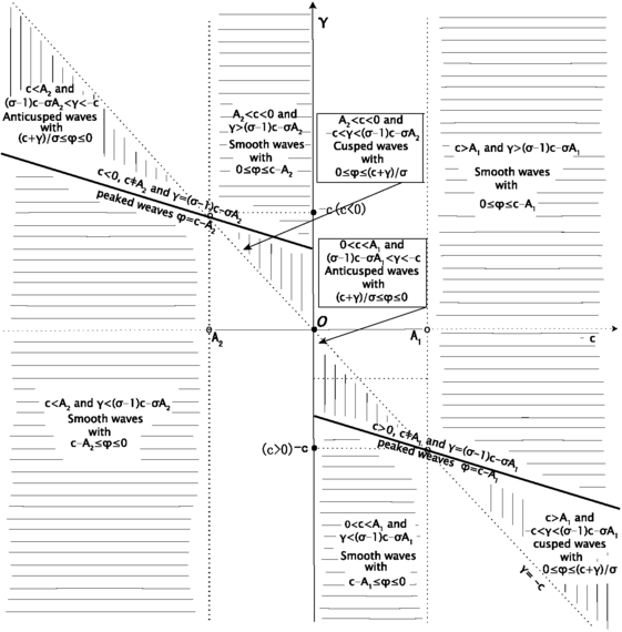

    

    The case 0<σ<1. In this case, there are four kind of waves: cuspons, anticuspons, peakons, and smooth waves. The 12 cases give rise to the subcategories of the categories 1–12 in Theorem 3.9, i.e. 1(2), 2(2), 3(2), 4(2), 5(2), 6(2), 7(2), 8(2), 9(2), 10(2), 11(2), and 12(2)

    Fig. 4

    

    The case σ=1. In this case, there are four kind of waves: cuspons, anticuspons, peakons and smooth waves. The 12 cases give rise to the subcategories of the categories 1–12 in Theorem 3.9, i.e. 1(2), 2(3), 3(3), 4(3), 5(3), 6(2), 7(2), 8(3), 9(3), 10(3), 11(3), and 12(2)

  • (3) If σ>1, then φ>0. Moreover, we have the following.

  If γ>(σ−1)c−σA ₁, then the solitary waves are smooth and unique up to translation with max _x∈ℝ φ(x)=c−A ₁.

  If γ=(σ−1)c−σA ₁, then the solitary wave is peaked with $\max_{x\in\mathbb{R}}\varphi(x)=c-A_{1}=\frac{c+\gamma}{\sigma}$.

  If −c<γ<(σ−1)c−σA ₁, then the solitary waves are cusped with $\max_{x\in\mathbb{R}}\varphi(x)=\frac{c+\gamma}{\sigma}$ (see Fig. 5).

  Fig. 5

  

  The case σ>1. In this case, there are four kind of waves: cuspons, anticuspons, peakons and smooth waves. The 12 cases give rise to the subcategories of the categories 1–12 in Theorem 3.9, i.e. 1(3), 2(4), 3(3), 4(3), 5(4), 6(3), 7(3), 8(4), 9(3), 10(3), 11(4), and 12(3)

• 2. −c<γ=−A ₁.

  • (1) If σ<0, then there is a smooth wave φ>0 with max _x∈ℝ φ(x)=c−A ₁ and an anticusped wave φ<0 with $\min_{x \in\mathbb{R} }\varphi(x)=\frac{c+\gamma}{\sigma}$ (see Fig. 2).

  • (2) If 0<σ<1, then there is a smooth wave φ>0 with max _x∈ℝ φ(x)=c−A ₁ (see Fig. 3).

  • (3) If σ=1, then the solitary wave is peaked with $\max_{x\in\mathbb{R}}\varphi(x)=c-A_{1}=\frac{c+\gamma}{\sigma}$ (see Fig. 4).

  • (4) If σ>1, then the solitary wave is cusped with $\max_{x\in\mathbb{R}}\varphi(x)=\frac{c+\gamma}{\sigma}$ (see Fig. 5).

• 3. −c<γ<−A ₁.

  • (1) If σ<0, then there is a smooth wave φ>0 with max _x∈ℝ φ(x)=c−A ₁ and an anticusped wave φ<0 with $\min_{x\in\mathbb{R}}\varphi(x)=\frac{c+\gamma}{\sigma}$ (see Fig. 2).

  • (2) If 0<σ<1, then φ>0. Moreover, we have the following.

    If −c<γ<(σ−1)c−σA ₁, then the solitary waves are cusped with $\max_{x\in\mathbb{R}}\varphi(x)=\frac{c+\gamma}{\sigma}$.

    If γ=(σ−1)c−σA ₁, then the solitary wave is peaked with $\max_{x\in\mathbb{R}}\varphi(x)\allowbreak =c-A_{1}=\frac{c+\gamma}{\sigma}$.

    If γ>(σ−1)c−σA ₁, then the solitary waves are smooth and unique up to translation with max _x∈ℝ φ(x)=c−A ₁ (see Fig. 3).

  • (3) If σ≥1, then the solitary wave is cusped with $\max_{x\in\mathbb{R}}\varphi(x)=\frac{c+\gamma}{\sigma}$ (see Figs. 4 and 5).

• 4. −A ₁<γ<−c<0.

  • (1) If σ<0, then φ<0. Moreover, we have the following.

    If σ<0 and −A ₁<(σ−1)c<γ<−c, then there is a smooth wave φ<0 with min _x∈ℝ φ(x)=c−A ₁ and a cusped solitary waves with $\max_{x\in \mathbb{R}}\varphi(x)=\frac{c+\gamma}{\sigma}$.

    If σ<0 and −A ₁<γ≤(σ−1)c, then there is a smooth wave φ<0 with min _x∈ℝ φ(x)=c−A ₁ (see Fig. 2).

  • (2) If 0<σ<1, then φ<0. Moreover, we have the following.

    If (σ−1)c−σA ₁<γ<−c, then the solitary waves are anticusped with $\min_{x\in\mathbb{R}}\varphi(x)=\frac{c+\gamma}{\sigma}$.

    If γ=(σ−1)c−σA ₁, then the solitary wave is peaked with $\min_{x\in\mathbb{R}}\varphi(x)\allowbreak =\frac{c+\gamma}{\sigma}$.

    If γ<(σ−1)c−σA ₁, then the solitary waves are smooth and unique up to translation with min _x∈ℝ φ(x)=c−A ₁ (see Fig. 3).

  • (3) If σ≥1, then there is an anticusped solitary wave φ<0 with $\min_{x\in\mathbb{R}}\varphi(x)=\frac{c+\gamma}{\sigma}$ (see Figs. 4 and 5).

• 5. A ₁=γ<−c<0.

  • (1) If σ<0, then there is a smooth solitary wave φ<0 with min _x∈ℝ φ(x)=c−A ₁, and if σ<0 and (σ−1)c<γ there are cusped solitary waves with $\max_{x\in\mathbb{R}}\varphi(x)=\frac{c+\gamma}{\sigma}$ and a smooth wave φ<0 with min _x∈ℝ φ(x)=c−A ₁ (see Fig. 2).

  • (2) If 0<σ<1, then there is a smooth wave φ<0 with min _x∈ℝ φ(x)=c−A ₁ (see Fig. 3).

  • (3) If σ=1, then there is a peaked wave φ<0 with $\min_{x \in\mathbb{R}}\varphi(x)=\frac{c+\gamma}{\sigma}=c-A_{1}$ (see Fig. 4).

  • (4) If σ>1, then the solitary waves is anticusped with $\min_{x \in\mathbb{R}}\varphi(x)=\frac{c+\gamma}{\sigma}$ (see Fig. 5).

• 6. γ<−A ₁<−c<0.

  • (1) If σ<0 and (σ−1)c<γ<−A ₁, then there is a smooth wave φ<0 with min _x∈ℝ φ(x)=c−A ₁ and a cusped wave φ>0 with $\max_{x \in\mathbb{R}}\varphi(x)=\frac{c+\gamma}{\sigma}$ (see Fig. 2).

  • (2) If 0<σ≤1, then there is a smooth wave φ<0 with min _x∈ℝ φ(x)=c−A ₁ (see Figs. 3 and 4).

  • (3) If σ>1, then φ<0. Moreover, we have the following.

    If (σ−1)c−σA ₁<γ<−c, then the solitary waves are anticusped waves with $\min_{x\in\mathbb{R}}\varphi(x)=\frac{c+\gamma}{\sigma}$.

    If γ=(σ−1)c−σA ₁, then the solitary wave is peaked with $\min_{x\in\mathbb{R}}\varphi(x)\allowbreak =c-A_{1}=\frac{c+\gamma}{\sigma}$.

    If γ<(σ−1)c−σA ₁, then there is a smooth wave φ<0 with min _x∈ℝ φ(x)=c−A ₁ (see Fig. 5).

• 7. γ<−A ₂<−c.

  • (1) If σ<0, then there is a smooth wave φ>0 with min _x∈ℝ φ(x)=c−A ₂ and a cusped wave φ>0 with $\max_{x\in\mathbb{R}}\varphi(x)=\frac{c+\gamma}{\sigma}$ (see Fig. 2).

  • (2) If 0<σ≤1, then there is a smooth wave φ<0 with min _x∈ℝ φ(x)=c−A ₂ (see Figs. 3 and 4).

  • (3) If σ>1, then φ<0. Moreover, we have the following.

    If γ<(σ−1)c−σA ₂, then the solitary waves are smooth and unique up to translation with min _x∈ℝ φ(x)=c−A ₂.

    If γ=(σ−1)c−σA ₂, then the solitary wave is peaked with $\min_{x\in\mathbb{R}}\varphi(x)\allowbreak =c-A_{2}=\frac{c+\gamma}{\sigma}$.

    If (σ−1)c−σA ₂<γ<−c, then the solitary waves are anticusped with $\min_{x\in\mathbb{R}}\varphi(x)=\frac{c+\gamma}{\sigma}$ (see Fig. 5).

• 8. γ=−A ₂<−c.

  • (1) If σ<0, then there is a smooth wave φ<0 with min _x∈ℝ φ(x)=c−A ₂, and a cusped wave φ>0 with $\max_{x \in\mathbb{R} }\varphi(x)=\frac{c+\gamma}{\sigma}$ (see Fig. 2).

  • (2) If 0<σ<1, then there is a smooth wave φ<0 with min _x∈ℝ φ(x)=c−A ₂ (see Fig. 3).

  • (3) If σ=1, then the solitary wave is peaked with $\min_{x\in\mathbb{R}}\varphi(x)=c-A_{2}=\frac{c+\gamma}{\sigma}$ (see Fig. 4).

  • (4) If σ>1, then the solitary wave is anticusped with $\min_{x\in\mathbb{R}}\varphi(x)=\frac{c+\gamma}{\sigma}$ (see Fig. 5).

• 9. −A ₂<γ<−c.

  • (1) If σ<0, then there is a smooth wave φ<0 with min _x∈ℝ φ(x)=c−A ₂ and a cusped wave φ>0 with $\max_{x\in\mathbb{R}}\varphi(x)=\frac{c+\gamma}{\sigma}$ (see Fig. 2).

  • (2) If 0<σ<1, then φ<0. Moreover, we have the following.

    If (σ−1)c−σA ₂<γ<−c, then the solitary waves are anticusped with $\min_{x\in\mathbb{R}}\varphi(x)\allowbreak =\frac{c+\gamma}{\sigma}$.

    If γ=(σ−1)c−σA ₂, then the solitary wave is peaked with $\min_{x\in\mathbb{R}}\varphi(x)=c-A_{2}=\frac{c+\gamma}{\sigma}$.

    If γ<(σ−1)c−σA ₂, then the solitary waves are smooth and unique up to translation with min _x∈ℝ φ(x)=c−A ₂ (see Fig. 3).

  • (3) If σ≥1, then the solitary wave is anticusped with $\min_{x\in\mathbb{R}}\varphi(x)=\frac{c+\gamma}{\sigma}$ (see Figs. 4 and 5).

• 10. 0<−c<γ<−A ₂.

  • (1) If σ<0, then φ>0. Moreover, we have the following.

    If σ<0 and −c<γ<(σ−1)c<−A ₂, then there is a smooth wave φ>0 with max _x∈ℝ φ(x)=c−A ₂ and an anticusped solitary waves with $\min_{x\in\mathbb{R}}\varphi(x)=\frac{c+\gamma}{\sigma}$.

    If σ<0 and (σ−1)c≤γ<−A ₂, then there is a smooth wave φ>0 with max _x∈ℝ φ(x)=c−A ₂ (see Fig. 2).

  • (2) If 0<σ<1, then φ>0. Moreover, we have the following.

    If −c<γ<(σ−1)c−σA ₂, then the solitary waves are cusped with $\max_{x\in\mathbb{R}}\varphi(x)=\frac{c+\gamma}{\sigma}$.

    If γ=(σ−1)c−σA ₂, then the solitary wave is peaked with $\max_{x\in\mathbb{R}}\varphi(x)\allowbreak =\frac{c+\gamma}{\sigma}$.

    If (σ−1)c−σA ₂<γ, then the solitary waves are smooth and unique up to translation with max _x∈ℝ φ(x)=c−A ₂ (see Fig. 3).

  • (3) If σ≥1, then there is a cusped solitary wave φ>0 with $\max_{x\in\mathbb{R}}\varphi(x)=\frac{c+\gamma}{\sigma}$ (see Figs. 4 and 5).

• 11. 0<−c<γ=A ₂.

  • (1) If σ<0, then there is a smooth solitary wave φ>0 with max _x∈ℝ φ(x)=c−A ₂, and if σ<0 and γ<(σ−1)c there are anticusped solitary waves with $\min_{x\in\mathbb{R}}\varphi(x)=\frac{c+\gamma}{\sigma}$ and a smooth wave φ>0 with max _x∈ℝ φ(x)=c−A ₂ (see Fig. 2).

  • (2) If 0<σ<1, then there is a smooth wave φ>0 with max _x∈ℝ φ(x)=c−A ₂ (see Fig. 3).

  • (3) If σ=1, then there is a peaked wave φ>0 with $\max_{x \in\mathbb{R}}\varphi(x)=\frac{c+\gamma}{\sigma}=c-A_{2}$ (see Fig. 4).

  • (4) If σ>1, then the solitary waves is cusped with $\max_{x \in\mathbb{R}}\varphi(x)=\frac{c+\gamma}{\sigma}$ (see Fig. 5).

• 12. 0<−c<−A ₂<γ.

  • (1) If σ<0 and −A ₂<γ<(σ−1)c, then there is a smooth wave φ>0 with max _x∈ℝ φ(x)=c−A ₂ and an anticusped wave φ<0 with $\min_{x \in\mathbb{R}}\varphi(x)=\frac{c+\gamma}{\sigma}$ (see Fig. 2).

  • (2) If 0<σ≤1, then there is a smooth wave φ>0 with max _x∈ℝ φ(x)=c−A ₂ (see Figs. 3 and 4).

  • (3) If σ>1, then φ>0. Moreover, we have the following.

    If −c<γ<(σ−1)c−σA ₂, then the solitary waves are cusped waves with $\max_{x\in\mathbb{R}}\varphi(x)=\frac{c+\gamma}{\sigma}$.

    If γ=(σ−1)c−σA ₂, then the solitary wave is peaked with $\max_{x\in\mathbb{R}}\varphi(x)\allowbreak =c-A_{2}=\frac{c+\gamma}{\sigma}$.

    If γ>(σ−1)c−σA ₂, then there is a smooth wave φ>0 with max _x∈ℝ φ(x)=c−A ₂ (see Fig. 5).

• 13. c=A ₁.

  • (1) If γ>−A ₁ and σ<0, then there is an anticusped wave φ<0 with $\min_{x \in\mathbb{R}}\varphi(x)=\frac{c+\gamma}{\sigma}$.

  • (2) If (σ−1)A ₁<γ<−A ₁, then the solitary waves are cusped with $\max_{x\in\mathbb{R}}\varphi(x)=\frac{c+\gamma}{\sigma}$ (see Fig. 2).

• 14. c=A ₂.

  • (1) If γ<−A ₂ and σ<0, then there is a cusped wave φ>0 with $\max_{x \in\mathbb{R}}\varphi(x)\allowbreak =\frac{c+\gamma}{\sigma}$.

  • (2) If −A ₂<γ<(σ−1)A ₂, then the solitary waves are anticusped with $\min_{x\in\mathbb{R}}\varphi(x)=\frac{c+\gamma}{\sigma}$ (see Fig. 2).

Moreover, each kind of the above solitary waves is unique and even up to translation. All solitary waves decay exponentially to zero at infinity.

We enclose the proof of this theorem as an Appendix for conciseness.

Remark 3.10

The peakons are solitons, which is a self-reinforcing solitary wave (a wave packet or pulse) that maintains its shape while it travels at constant speed. Solitons are caused by a cancelation of nonlinear and dispersive effects in the medium (Constantin 2011). They replicate a characteristic of the traveling waves of greatest height-exact traveling solutions of the governing equations for water waves with a peak at their crest. The concept of peakon was introduced by Camassa and Holm (1993). The way a smooth initial condition breaks up into a train of peakons is by limiting to a verticality at each inflection point with negative slope, from which a derivative discontinuity emerges (see the blow-up mechanism in Sect. 4) (Camassa and Holm 1993).

Remark 3.11

The peakons and cuspons are both physical solutions. Indeed, breaking waves, both whitecaps and surf, are commonly observed in the ocean (therefore the cuspon is physical solution since for a cuspon φ we have lim _y↑x φ _x (y)=−lim _y↓x φ _x (y)=±∞). Moreover, when initiated by earthquakes, these waves may turn into formidable shallow-water breaking wave phenomenon, the tsunami. A tsunami wave is generated when a large body of water, such as a region in a lake or a sea, becomes rapidly displaced on a massive scale. With typical wavelengths of 200 km, tsunamis are governed by shallow water equations and can be catastrophic when they reach land, as seen in the recent Indonesia and Japan earthquakes (Constantin 2011).

Remark 3.12

To our knowledge, there are two approach to study stability. One is the variational approach, that is, it should be proved that each peakon is the unique minimum (ground state) of constrained energy, from which its orbital stability is proved (Constantin and Molinet 2001). Another approach to study stability is to linearize the equation around the solitary waves, and it is commonly believed that nonlinear stability is governed by the linearized equation. However, for the Dullin–Gottwald–Holm system, the nonlinearity plays the dominant role rather than being a higher-order correction to linear terms. Thus it is unclear how one can get nonlinear stability of peakons by studying the linearized problem. Moreover, the peakons are not differentiable, making it difficult to analyze the spectrum of the linearized operator around them.

We think one possible approach to establish the stability of the peakons for the GDGH2 system is due to Constantin and Strauss (2000), Lin and Liu (2009) for the Degasperis–Procesi equation). To extend the approach to nonlinear stability of the GDGH2 peakons, our main difficulty is: by expanding the energy E (given by (1.6) in the introduction) around the peakon, the error term is in the form of the difference of the maxima of peakon and the perturbed solution. Then how to estimate this error term?

We will study the orbital stability of the smooth solitary waves of the GDGH2 system using the classical method provided by Grillakis et al. (1987).

In view of the length of this paper, we will discuss the stability of smooth solitary waves and peakons in a forthcoming paper.

Though there is no explicit expression for φ, and so η in view of (3.10), as in Zhang and Liu (2010), the effects of the traveling speed c on the function φ can be analyzed to provide some general description of its profile. Similarly to the case in Zhang and Liu (2010) we have

Proposition 3.13

Assume (3.16) holds and φ is a smooth solitary wave of (3.1) as obtained in Theorem 3.7. Then ∂ _c φ decays exponentially to zero at infinity and has at most two zeros on ℝ. In particular, if −A ₁<γ<A and $A_{1}<c<\frac{1}{A-\gamma}$, then ∂ _c φ has exactly two zeros on ℝ.

Proof

Again we only discuss the case c>A ₁. The other cases can be handled similarly.

Denote ω=∂ _c φ. The exponential decay of ω can be inferred from (A.2). Since φ is unique and even up to translations, we may assume that φ(0)=c−A ₁. Hence ω(0)=1 and ω is even. Assume ω(x ₀)=0 for some x ₀>0. Differentiating (3.24) with respect to c and evaluating at x=x ₀, we get

where use has been made of c+γ−σφ>0. Since φ _x (x ₀)<0, we deduce from the above inequality that ω _x (x ₀)<0. Therefore ω is strictly decreasing near x ₀. It is then inferred from the continuity of ω that it has at most two zeros on ℝ.

If −A ₁<γ<A and $A_{1}<c<\frac{1}{A-\gamma}$, then we have (−A−γ)c ²+2c−γ>0. Using the decay estimate (A.2) we see that φ decays faster at infinity as c gets larger, since

$$\partial_{c} \biggl(\frac{\sqrt{c^{2}+Ac-1}}{\sqrt{c(c+\gamma)}} \biggr) =\frac{(-A-\gamma)c^{2}+2c-\gamma}{(c(c+\gamma))^{3/2}\sqrt{c^{2}+Ac-1}}>0, $$

we know ω(x)<0 at infinity and ω has at least two zeros. Combining the above argument we proved that ω(x) has exactly two zeros ±x ₀ in this case.

Next we try to find an implicit formula for the peaked solitary waves. Let us consider only the case −c<−A ₁<γ. By Theorem 3.7 we know that peaked solitary waves exist only when γ=(σ−1)c−σA ₁. In this case we have

$$\varphi_{x}^{2}=\frac{\varphi^{2}(c-A_{2}-\varphi)}{c-\varphi}. $$

Since φ is positive, even with respect to some x ₀ and decreasing on (x ₀,∞), so for x>x ₀ we have

$$\varphi_{x}=-\varphi\sqrt{1-\frac{A_{2}}{c-\varphi}}. $$

Integrating we get

$$-(x-x_{0})=\int_{c-A_{1}}^{\varphi} \frac{\mathrm{d}t}{t\sqrt{1-\frac{A_{2}}{c-t}}}. $$

Let $\omega=1-\frac{A_{2}}{c-t}$ in the above equation; then

Therefore we obtain an implicit formula for the peaked solitary waves:

$$ -|x-x_{0}|= \biggl(\sqrt{\frac{c}{c-A_{2}}}\ln \biggl \vert \frac{\sqrt{c\omega }-\sqrt{c-A_{2}}}{\sqrt{c\omega} +\sqrt{c-A_{2}}}\biggr \vert -\ln \biggl \vert \frac{\sqrt{\omega}-1}{\sqrt{\omega}+1} \biggr \vert \biggr)_{1-\frac{A_{2}}{A_{1}}}^{1-\frac{A_{2}}{c-\varphi}}. $$

(3.29)

 □

4 Wave-Breaking Phenomena

In this section, we study the blow-up problem for the GDGH system (1.5). For convenience, we rewrite system (1.5) as the following conservation law form (see also system (3.6)):

$$ \everymath{\displaystyle} \begin{cases} &u_t + (\sigma u- \gamma) u_x = -\partial_x p \ast \biggl[ (\gamma-A) u + \frac{3 -\sigma}{2} u^2 + \frac{\sigma}{2} u_x^2 + \frac{1}{2} \rho^2 \biggr],\\ &\rho_t + u\rho_x = - \rho u_x. \end{cases} $$

(4.1)

4.1 Blow-up Scenario

Using the Littlewood–Paley analysis for the transport equation and Moser-type estimates, Gui and Liu proved the following lemma in Gui and Liu (2010) to handle the regularity of solutions to the model (1.2). We recall this proposition for completeness.

Proposition 4.1

(Gui and Liu 2010)

Let 0<σ<1. Suppose that f ₀∈H ^σ,g∈L ¹([0,T];H ^σ), v,∂ _x v∈L ¹([0,T];L ^∞) and that $f \in L^{\infty} ([0,T]; H^{\sigma} ) \cap C ( [0,T]; \mathcal{S'} )$ solves the 1-dimensional linear transport equation

$$\begin{cases} \partial_t f + v\partial_x f = g,\\ f|_{t=0} = f_0. \end{cases} $$

Then f∈C([0,T];H ^σ). Moreover, to state it precisely, there exists a constant C depending only on σ and such that the following statement holds:

$$\bigl\| f(t) \bigr\|_{H^{\sigma}} \leq \| f_0 \|_{H^{\sigma}} + C\int _0^t \bigl\| g(\tau) \bigr\|_{H^{\sigma}} \,\mathrm{d}\tau+ C \int _0^t \bigl\| f(\tau) \bigr\|_{H^{\sigma}} V'(\tau) \,\mathrm{d}\tau $$

or, hence,

$$\bigl\| f(t) \bigr\|_{H^{\sigma}} \leq \mathrm{e}^{CV(t)} \biggl(\| f_0 \|_{H^{\sigma}} + C \int_0^t \bigl\| g(\tau) \bigr\|_{H^{\sigma}}\,\mathrm{d}\tau \biggr) $$

with $V(t) = \int_{0}^{t} ( \|v(\tau)\|_{L^{\infty}} + \|\partial_{x} v(\tau)\|_{L^{\infty}} ) \,\mathrm{d}\tau$.

The two equations for u and ρ in system (4.1) are of a transport structure,

$$\partial_t f + v \partial_x f =g. $$

It is well known that most of estimates are available when v has enough regularity. Roughly speaking, the regularity of the initial data is expected to be preserved as soon as v belongs to L ¹(0,T;Lip). More specifically, u and ρ are “transported” along directions of u−γ and u, respectively. Thus, the solution can be estimated in a Gronwall way involving $\| u_{x} \|_{L^{\infty}}$. Hence, we can use these estimates and Proposition 4.1 to derive the following blow-up criterion. The detailed proof can be found in Gui and Liu (2010).

Theorem 4.2

Assume (u,ρ) is the solution of system (4.1) with initial data (u ₀,ρ ₀−1)∈H ^s×H ^s−1,s≥2, and let T be the maximal time of existence. Then

$$T<\infty\quad\Rightarrow\quad\int_0^T \bigl\|u_x(\tau)\bigr\|_{L^{\infty}} \,\mathrm{d}\tau= \infty. $$

Based on the above result, we can establish the following theorem on the precise blow-up mechanism. It is shown that the solution to the model (4.1) can only have singularities which correspond to wave breaking.

Theorem 4.3

(Wave-breaking criterion)

Let (u ₀,ρ ₀−1)∈H ^s×H ^s−1 with s≥2, and T>0 be the maximal time of existence of the solution (u,ρ) to system (4.1) with initial data (u ₀,ρ ₀). Then the corresponding solution (u,ρ) blows up in finite time if and only if

$$ \lim_{t\uparrow T} \Bigl[ \inf_{x\in \mathbb{R}} \sigma u_x(t,x) \Bigr] = -\infty. $$

(4.2)

Since the proof of this result is essentially similar to Theorem 3.4 in Chen and Liu (2011), so we omit it here.

4.2 Wave-Breaking Phenomena

We next give two conditions, which can guarantee wave-breaking phenomena in finite time. We will use the following two associated Lagrangian scales of the GDGH system (4.1), namely:

$$ \begin{cases} \displaystyle \frac{\partial q_1}{\partial t} = \sigma u(t,q_1) - \gamma,\quad 0<t<T,\\ q_1(0,x) = x,\quad x \in \mathbb{R}\end{cases} $$

(4.3)

and

$$ \begin{cases} \displaystyle \frac{\partial q_2}{\partial t} = u(t,q_2),\quad0<t<T,\\ q_2(0,x) = x,\quad x \in \mathbb{R}, \end{cases} $$

(4.4)

where u∈C ¹([0,T),H ^s−1) is the first component of the solution (u,ρ) to system (4.1) with initial data (u ₀,ρ ₀−1)∈H ^s×H ^s−1 (s≥2), and T>0 is the maximal time of existence. By a direct calculation, we have

$$\displaystyle q_{1,tx}(t,x) = \sigma u_x \bigl(t, q_1(t,x) \bigr) q_{1,x} (t,x) $$

and

$$\quad q_{2,tx}(t,x) = u_x \bigl(t, q_2(t,x) \bigr) q_{2,x} (t,x). $$

Then,

$$q_{1,x} (t,x) = \mathrm{e}^ {\sigma\int_0^t u_x ( \tau, q_1(\tau,x) ) \,\mathrm{d}\tau} >0,\quad\text{for}\ t>0, x\in \mathbb{R}$$

and

$$q_{2,x} (t,x) = \mathrm{e}^ {\int_0^t u_x ( \tau, q_2(\tau,x) ) \,\mathrm{d}\tau} >0,\quad\text{for}\ t>0, x\in \mathbb{R}, $$

which means that q _i (t,⋅):ℝ→ℝ (i=1,2) are two diffeomorphisms of the line for every t∈[0,T). Consequently, the L ^∞-norm of any function v(t,⋅)∈L ^∞ (t∈[0,T) is preserved under the family of these two diffeomorphisms q _i (t,⋅) (i=1,2), i.e.,

$$\bigl\| v(t,\cdot) \bigr\|_{L^{\infty} } = \bigl\| v \bigl( t, q_1(t,\cdot) \bigr) \bigr\|_{L^{\infty}} = \bigl\| v \bigl( t, q_2(t,\cdot) \bigr) \bigr\|_{L^{\infty}},\quad t\in[0,T). $$

Similarly,

$$\inf_{x\in \mathbb{R}} v(t,x) = \inf_{x\in \mathbb{R}} v \bigl(t,q_1(t,x) \bigr) =\inf_{x\in \mathbb{R}} v \bigl(t,q_2(t,x) \bigr),\quad t\in[0,T) $$

and

$$\sup_{x\in \mathbb{R}} v(t,x) = \sup_{x\in \mathbb{R}} v \bigl(t,q_1(t,x) \bigr) =\sup_{x\in \mathbb{R}} v \bigl(t,q_2(t,x) \bigr),\quad t\in[0,T). $$

We recall the following useful lemma established by Constantin and Escher.

Lemma 4.4

(Constantin and Escher 1998a)

Let T>0 and v∈C ¹([0,T);H ²). Then for every t∈[0,T), there exists at least one point ξ(t)∈ℝ with

$$m_1 (t) := \inf_{x\in \mathbb{R}} \bigl[v_x(t,x)\bigr] = v_x \bigl(t,\xi(t)\bigr), $$

and the function m(t) is almost everywhere differentiable on (0,T) with

$$ \frac{\mathrm{d} m_1 }{\mathrm{d}t} = v_{tx}\bigl(t,\xi(t)\bigr) \quad \mbox{\textit{a.e. on}}\ (0,T). $$

(4.5)

We are in the position to give the first blow-up result.

Theorem 4.5

Let σ>0. Assume (u ₀,ρ ₀−1)∈H ^s×H ^s−1 with s≥2. If there is some x ₀∈ℝ such that

$$ \rho_0 (x_0) =0,\quad u_{0,x} (x_0) = \inf_{x\in \mathbb{R}} u_{0,x} (x) $$

(4.6)

and one of the following two conditions holds:

(4.7)

$$ u_{0,x} (x_0) < -\frac{C_2}{\sqrt{\sigma}}. $$

(4.8)

Then the corresponding solution (u,ρ) to system (4.1) blows up in finite time in the following sense: there is a T ₁ with

$$ 0< T_1 \leq2 + \frac{4 (1 - \varepsilon_0 ) (1 + |u_{0,x}(x_0)| ) }{\varepsilon_0 (1- \varepsilon_0) - [C_1 (1 - \varepsilon_0 ) + |\gamma-A|^2 ] \|(u_0,\rho_0-1) \|^2_{H^1 \times L^2}}, $$

(4.9)

$$ 0< T_1 \leq\frac{1}{C_2 \sqrt{\sigma}} \ln\frac{\sqrt{\sigma}u_{0,x}(x_0) - C_2}{\sqrt{\sigma}u_{0,x}(x_0) + C_2} $$

(4.10)

respectively, such that

$$\liminf_{t \uparrow T_1} \Bigl( \inf_{x\in \mathbb{R}} u_x(t,x) \Bigr) = -\infty, $$

where

$$C_1 = 2 |3-\sigma| + 2 \sigma, $$

$$C_2 = \biggl( |3-\sigma| + \frac{|\gamma-A|^2+ \sigma}{2 } \biggr)^{\frac{1}{2}} \bigl\| ( u_0, \rho-1 ) \bigr\|_{H^1 \times L^2} $$

and

$$ \varepsilon_0 = \frac{|\gamma- A|^2 +C_1 - |\gamma-A| \sqrt {|\gamma- A|^2 +C_1}}{C_1} $$

(4.11)

is the maximum point of the function

$$ g( \varepsilon) = \displaystyle\frac{\varepsilon (1 - \varepsilon)}{C_1 (1-\varepsilon) + |\gamma-A|^2 }. $$

(4.12)

Proof

By Theorem 3.2 and a simple density argument, we need only to prove this theorem for s≥3. We may also assume u ₀≠0, otherwise it is trivial. Let T>0 be the maximal time of existence of the corresponding solution (u,ρ) to system (4.1).

By Lemma 4.4, we can define m ₁(t) and ξ(t) as

$$ m_1 (t) = u_x \bigl(t,\xi(t)\bigr) = \inf_{x\in \mathbb{R}} u_x(t,x),\quad t\in [0,T). $$

(4.13)

Obviously

$$ u_{xx} \bigl(t,\xi(t)\bigr) =0, \quad\text{a.e.}\ t\in[0,T). $$

(4.14)

Since q ₂(t,⋅) defined by (4.4) is a diffeomorphism of the line for any t∈[0,T), there exists a x ₁(t)∈ℝ such that

$$ q_2 \bigl(t,x_1(t)\bigr) = \xi(t),\quad t\in[0,T). $$

(4.15)

Along the trajectory of q ₂(t,x ₁(t)), we have

$$ \frac{\mathrm{d}\rho(t,\xi(t))}{\mathrm{d}t} = - \rho \bigl(t, \xi(t) \bigr) u_x \bigl(t, \xi(t)\bigr). $$

(4.16)

Equations (4.6) and (4.13) imply that

$$ m_1 (0) = u_x\bigl(0,\xi(0)\bigr) = \inf_{x \in \mathbb{R}} u_{0,x} (x) = u_{0,x} (x_0), $$

(4.17)

hence we can choose ξ(0)=x ₀ and ρ ₀(ξ(0))=ρ ₀(x ₀)=0, and then from (4.16) it follows that

$$ \rho\bigl(t,\xi(t)\bigr) \equiv0, \quad\text{for}\ t\in[0,T). $$

(4.18)

Using the identity $-\partial_{x}^{2} p\ast f = f - p\ast f$, for any f∈L ², by differentiating the first equation in (4.1) with respect to x we obtain

(4.19)

Let

$$ f = \frac{ 3-\sigma}{2} u^2 - (\gamma-A) \partial_x^2 p \ast u - p \ast \biggl( \frac{ 3-\sigma}{2} u^2 + \frac{\sigma}{2} u_x^2 + \frac{1}{2} \rho^2 \biggr). $$

(4.20)

Hence, along the trajectory q ₂(t,x ₁(t)), for t∈[0,T), noting (4.14), we have

$$ m_1'(t) = -\frac{\sigma}{2} m_1^2 + f \bigl(t, \xi(t) \bigr), $$

(4.21)

where “′” is the derivative with respect to t.

We first prove the case (4.7). Toward this goal, let us now estimate the upper bound for f. Since $\partial_{x}^{2} p\ast u = \partial_{x} p \ast \partial_{x} u$, we have

(4.22)

By the Sobolev embedding theorem, we have

$$ u^2 \leq\frac{1}{2} \bigl(\|u\|_{L^2}^2 + \|u_x\|_{L^2}^2 \bigr). $$

(4.23)

Using Young’s inequality, we deduce that

$$ |\gamma-A| | p_x \ast u_x | \leq\frac{1}{2} |\gamma-A| \|u_x\|_{L^2 } \leq\frac{1 - \varepsilon_0}{4} + \frac{|\gamma-A|^2}{4(1 - \varepsilon_0) } \|u_x\|_{L^2}^2, $$

(4.24)

where ε ₀ is defined by (4.11),

$$ \biggl \vert p \ast \biggl( \frac{ 3-\sigma}{2} u^2 + \frac {\sigma}{2} u_x^2 \biggr) \biggr \vert \leq \frac{1}{2} \biggl \Vert \frac{ 3-\sigma}{2} u^2 + \frac{\sigma}{2} u_x^2 \biggr \Vert _{L^1} \leq \frac{ |3-\sigma|}{4} \|u\|_{L^2}^2 + \frac{\sigma}{4} \|u_x\|_{L^2}^2 $$

(4.25)

and

$$ \bigl|p \ast(\rho-1) \bigr| \leq\| p \|_{L^2} \|\rho-1\|_{L^2} = \frac{1}{2} \|\rho-1\|_{L^2} \leq\frac{1}{4} + \frac{1}{4} \|\rho-1 \|_{L^2}^2. $$

(4.26)

Substituting the above four estimates (4.23)–(4.26) back into (4.22), we arrive at

for (t,x)∈[0,T)×ℝ. We claim that

$$C_3 >0. $$

Indeed, since ε ₀ is the maximum point of the function g(ε), it is inferred that

and (4.7) reduces to

$$\bigl\| ( u_0, \rho-1 ) \bigr\|^2_{H^1 \times L^2} < g ( \varepsilon_0). $$

In view of the definitions of C ₃ and g(ε ₀), it follows that

Now by (4.21) it is deduced that

$$ m_1'(t) \leq-\frac{\sigma}{2} m_1^2(t) -C_3 \leq-C_3 <0,\quad t\in[0,T), $$

(4.27)

which shows that m ₁(t) is strictly decreasing in [0,T). If the solution (u,ρ) to (4.1) exists globally in time, i.e. T=∞, we will derive a contradiction. Define

$$ t_1 = \frac{1 + |u_{0,x} (x_0)|}{C_3}. $$

(4.28)

Integrating (4.27) over [0,t ₁] yields

$$m_1 (t_1) \leq m_1 (0) + \int _0^{t_1} m_1'(t) \,\mathrm{d}t \leq \bigl|u_{0,x} (x_0)\bigr| - C_3 t_1 = -1, $$

where we have used (4.17). Therefore

$$ m_1 (t) \leq-1 \quad\text{on}\ [t_1, T). $$

(4.29)

We also get from (4.27) that $m_{1}'(t) \leq-\frac{\sigma}{2} m_{1}^{2}(t)$ on [t ₁,T), i.e.,

$$-\frac{\mathrm{d}}{\mathrm{d}t} \biggl( \frac{1}{m_1(t)} \biggr) \leq- \frac{\sigma}{2},\quad\text{for}\ t\in[t_1,T). $$

Integrating this inequality and taking into account (4.29) lead to

$$- \frac{1}{m_1(t)} -1 \leq- \frac{1}{m_1(t)} + \frac{1}{m_1(t_1)} \leq-\frac{\sigma}{2} (t-t_1), \quad\text{for}\ t\in[t_1,T), $$

hence

$$ m_1(t) \leq\frac{2}{{\sigma}(t-t_1) -2} \rightarrow- \infty,\quad \text{as}\ t\uparrow t_1 + \frac{2}{\sigma}, $$

(4.30)

which implies $T \leq t_{1} + \frac{2}{\sigma}$; this is a contradiction since T equals ∞.

We next prove the case (4.8). Instead of (4.24), we use the following estimate:

(4.31)

Combing (4.23), (4.25)–(4.26) and (4.31), it is easy to find that

$$ f \leq \biggl( \frac{|3-\sigma|}{2} + \frac{|\gamma-A|^2+ \sigma}{ 4 } \biggr) \bigl\| ( u_0, \rho-1 ) \bigr\|^2_{H^1 \times L^2} = \frac{1}{2} C_2^2. $$

(4.32)

From (4.21), we deduce that

$$ m_1'(t) \leq-\frac{\sigma}{2} m_1^2(t) + \frac{1}{2} C_2^2,\quad t\in [0,T). $$

(4.33)

If $m_{1} (0) = u_{0,x} (x_{0}) < - \frac{C_{2}}{\sqrt{\sigma}}$, we now claim that

$$ m_1 (t) < -\frac{C_2}{\sqrt{\sigma}}, \quad\forall t \in[0,T). $$

(4.34)

In fact, as $m_{1}(0) < -\frac{C_{2}}{\sqrt{\sigma}}$ and m ₁(t) is continuous, failure of (4.34) would ensure the existence of some t ₀∈(0,T) such that $m_{1}(t) < -\frac{C_{2}}{\sqrt{\sigma}}$ on [0,t ₀), while $m_{1} (t_{0}) = - \frac{C_{2}}{\sqrt{\sigma}}$. But then we would have by (4.33)

$$\frac{\mathrm{d}m_1 (t)}{\mathrm{d}t} <0, \quad\text{a.e.}\ t \in(0,t_0). $$

Being locally Lipshitz, the function m ₁(t) is absolutely continuous on [0,t ₀], and therefore an integration of the previous inequality would lead to

$$m_1 (t_0) \leq m_1 (0) < - \frac{C_2}{\sqrt{\sigma}}, $$

which contradicts our assumption $m_{1} (t_{0}) = - \frac{C_{2}}{ \sqrt{\sigma}}$.

Solving the inequality (4.33) gives

$$\frac{\sqrt{\sigma} m_1 (0)+ C_2}{\sqrt{\sigma} m_1 (0) - C_2} \mathrm{e}^{C_2 \sqrt{\sigma} t} -1 \leq\frac{ 2 C_2}{\sqrt{\sigma} m_1 (t)+ C_2} \leq0. $$

In view of $0< \frac{\sqrt{\sigma} m_{1} (0)+ C_{2}}{ \sqrt {\sigma} m_{1} (0)- C_{2})} < 1$, we deduce that there exists T ₁ satisfying

$$0<T_1< \frac{1}{C_2 \sqrt{\sigma}} \ln\frac{\sqrt{\sigma} m_1 (0)- C_2}{\sqrt{\sigma} m_1 (0)+ C_2} $$

such that $\lim_{t\uparrow T_{1}} m(t) = -\infty$. This completes the proof of Theorem 4.5. □

Corollary 4.6

Under the assumptions of Theorem 4.5, assume further that $s> \frac{5}{2}$. Then there exists a T ₂ with 0<T ₁≤T ₂ (T ₁ is defined in (4.9) and (4.10)) such that

Proof

We only prove the case (4.7), since the other case is similar.

Differentiating the second equation in (4.1) with respect to x, evaluating it along the trajectory q ₂(t,x), we obtain

$$ \frac{\mathrm{d}\rho_x (t,q_2(t,x) )}{\mathrm{d}t} = - u_{xx} \bigl(t,q_2(t,x) \bigr) \rho \bigl(t,q_2(t,x) \bigr) - 2 u_x \bigl(t,q_2(t,x) \bigr) \rho_x \bigl(t,q_2(t,x) \bigr). $$

(4.35)

Take x=x ₁(t) (defined by (4.15)), in view of the fact u _xx (t,ξ(t))=0 for a.e. t∈[0,T), one infers from (4.35) that

$$\frac{\mathrm{d}\rho_x (t,\xi(t) )}{\mathrm{d}t} = -2 u_x \bigl(t,\xi(t) \bigr) \rho_x \bigl(t,\xi(t) \bigr), $$

where ξ(t)=q ₂(t,x ₁(t)). Recall (4.13); by integrating one obtains

$$\rho_x \bigl(t,\xi(t) \bigr) = \rho_{0,x}(x_0) \mathrm{e}^ {-2 \int_0^t u_x (\tau, \xi(\tau))\,\mathrm{d}\tau} = \rho_{0,x}(x_0) \mathrm{e}^ {-2 \int_0^t \inf_{x \in \mathbb{R}} u_x (\tau, x)\,\mathrm{d}\tau}. $$

Since m ₁(t) is strictly decreasing in [0,T), by (4.27) and (4.30) we have

(4.36)

where t ₁ is defined by (4.28). Obviously,

$$\lim_{t \uparrow t_1 + \frac{2}{\sigma} } \mathrm{e}^ {- \frac{4}{\sigma} \ln [ \sigma(t_1 -t) + 2 ] } = + \infty. $$

Therefore, if ρ _0,x (x ₀)>0, in view of Theorem 4.3, it is inferred that there exists some 0<T ₁≤T ₂ such that

$$\sup_{x\in \mathbb{R}} \rho_x (t,x) \geq\rho_x \bigl(t, \xi(t)\bigr) \rightarrow+ \infty $$

as t↑T ₂; if ρ _0,x (x ₀)<0, one can deduce (b) similarly. This completes the proof of Corollary 4.6. □

The second blow-up result we obtained is

Theorem 4.7

Let σ<0. Assume (u ₀,ρ ₀−1)∈H ^s×H ^s−1 (s≥2) and there exists some x ₁∈ℝ such that

$$ u_{0,x} (x_1) > \frac{C_4}{\sqrt{-\sigma}}, $$

(4.37)

where

$$C_4 = \biggl(2 + \frac{3 -\sigma + |\gamma-A|^2}{2} \biggr)^{\frac{1}{2}} \bigl\| ( u_0, \rho_0-1 ) \bigr\|_{H^1 \times L^2}. $$

Then there exists a T ₃ with

$$0 < T_3 \leq\frac{-2}{\sigma u_{0,x}(x_1) - \sqrt{C_4 (-\sigma)^ {\frac{3}{2}} u_{0,x} (x_1)}} $$

such that

$$\liminf_{t \uparrow T_3} \Bigl( \sup_{x\in \mathbb{R}} u_x(t,x) \Bigr) = \infty. $$

Proof

As in the proof of Theorem 4.5, we need only to prove this theorem for s≥3 and u ₀≠0. Let T>0 be the maximal time of existence of the corresponding solution (u,ρ) to system (4.1).

We now estimate the lower bound for f defined by (4.20). Similar to the proof of (4.32), one infers that

(4.38)

Since

$$\sup_{x\in \mathbb{R}} \bigl[ v_x(t,x) \bigr] = - \inf_{x\in \mathbb{R}} \bigl[ -v_x(t,x) \bigr] $$

and by Lemma 4.4, there exists at least a η(t)∈ℝ such that

$$ m_2 (t) =: u_x \bigl( t, \eta(t) \bigr) = \sup_{x\in \mathbb{R}} u_x(t,x), \quad\text{for}\ t\in[0,T). $$

(4.39)

Obviously,

$$u_{xx} \bigl(t,\eta(t)\bigr)=0,\quad\text{for a.e.}\ t\in[0,T). $$

Recall that q ₂(t,⋅) defined by (4.4) is a diffeomorphism of the line for any t∈[0,T), we see that there exists a x ₂(t)∈ℝ such that

$$ q_2 \bigl(t,x_2(t)\bigr) = \eta(t),\quad t\in[0,T). $$

(4.40)

Evaluating (4.19) along q ₂(t,x ₂(t)), in view of (4.38), we obtain

$$ m'_2(t) =- \frac{\sigma}{2} m_2^2 (t) + \frac{1}{2} \rho^2 \bigl(t,\eta(t)\bigr) + f\bigl(t,\eta(t)\bigr) \\ \geq-\frac{\sigma}{2} m_2^2 (t) - \frac{1}{2} C_4^2, \quad \text{for}\ t\in[0,T). $$

(4.41)

Equation (4.37) implies that $m_{2} (0) \geq u_{0,x}(x_{1}) > \frac{C_{4}}{\sqrt{-\sigma}}$; then from (4.41) it follows that $m_{2}'(0) >0$ and m ₂(t) is strictly increasing over [0,T). Therefore

$$ m_2(t) > m_2(0) \geq u_{0,x} (x_1) >0. $$

(4.42)

Let

$$\delta= \frac{1}{2} + \frac{1}{2} \sqrt{\frac{C_4}{u_{0,x}(x_1) \sqrt {-\sigma}}} \in \biggl(\frac{1}{2}, 1 \biggr). $$

By (4.42), it is inferred from (4.41) that

$$m_2'(t) \geq -\frac{\sigma}{2} m_2^2 (t) - \frac{1}{2} C_4^2 \geq-\frac{\sigma}{2} m_2^2 (t) \bigl[ 1 - (2\delta-1 )^4 \bigr] \geq- \delta\sigma m_2^2 (t), \quad\text{for}\ t\in[0,T). $$

Solving this inequality gives

$$m_2 (t) \geq\frac{u_{0,x}(x_1)}{ 1+ \delta\sigma u_{0,x} (x_1) t} \rightarrow\infty, \quad\text{as}\ t \rightarrow-\frac {1}{\delta\sigma u_{0,x}(x_1)}. $$

Consequently,

$$T \leq-\frac{1}{\delta\sigma u_{0,x}(x_1)}, $$

which is the desired result and completes the proof of the theorem. □

Remark 4.8

It should be pointed out that a “null condition” as (4.6) is not required in Theorem 4.7.

4.3 Lower Bound of the Lifespan

Attention is now turned to a lower bound depending only on $\| ( u_{0}, \rho_{0} -1 ) \|_{H^{1} \times L^{2}}$ and inf _x∈ℝ u _0,x (x) for the lifespan of the solution of system (4.1). We obtain the following result.

Theorem 4.9

Let σ>0. Assume that (u ₀,ρ ₀−1)∈H ^s×H ^s−1 with s≥2 and T _max>0 is the lifespan of the corresponding solution to (4.1). Assume further (4.6) holds, i.e., there is some x ₀∈ℝ such that

$$\rho_0 (x_0) =0,\quad u_{0,x} (x_0) = \inf_{x\in \mathbb{R}} u_{0,x} (x). $$

If T _max<∞, then the lifespan T _max>0 satisfies

$$ T_{\max} \geq T_4 = \frac{2}{C_5 \sqrt{\sigma}} \arctan \biggl( \frac{-C_5}{\sqrt{\sigma}\inf_{x \in \mathbb{R}} u_{0,x} (x)} \biggr), $$

(4.43)

where C ₅ is defined by

$$C_5 = \biggl(2 + |3 -\sigma| + \frac{\sigma+ |\gamma-A|^2}{2} \biggr)^{\frac{1}{2}} \bigl\| ( u_0, \rho_0 -1 ) \bigr\|_{H^1 \times L^2}. $$

Proof

For use during the proof, we derive a lower bound estimate of f defined by (4.20) for σ>0. Similar to the proof of (4.38), we have

$$ f \geq- \biggl( 1 + \frac{2|3 -\sigma| + \sigma+ |\gamma -A|^2}{4} \bigl\| ( u_0, \rho_0 -1 ) \bigr\|^2_{H^1 \times L^2} \biggr) = - \frac{1}{2} C_5^2. $$

(4.44)

Let us first assume that the initial data (u ₀,ρ ₀−1)∈H ^s×H ^s−1 (s≥3). Noting (4.44), from (4.21) it is inferred that

$$m_1'(t) = -\frac{\sigma}{2} m_1^2 + f \bigl(t, \xi(t) \bigr) \geq -\frac{\sigma}{2} m_1^2 - \frac{1}{2} C_5^2. $$

Integrating gives

$$\arctan\frac{\sqrt{\sigma}m_1(t)}{C_5} \geq\arctan \biggl( \frac {\sqrt{\sigma}m_1 (0)}{C_5} \biggr) - \frac{C_5 \sqrt{\sigma}}{2} t,\quad \forall t < \min \{ T_{\max}, T_4 \}, $$

or, which is the same,

$$m_1 (t) \geq\frac{C_5 \sqrt{\sigma}m_1(0) - C_5^2 \tan ( \frac{C_5 \sqrt{\sigma}}{2} t )}{C_5 \sqrt{\sigma}+ \sigma m_1 (0) \tan ( \frac{C_5 \sqrt{\sigma}}{2} t )}. $$

Consequently, due to (4.2), we deduce from the above inequality the desired result (4.43).

If s∈[2,3), it is easy to see that the lifespan $T^{s}_{\max}$ as a function of s for the initial data (u ₀,ρ ₀−1)∈H ^s×H ^s−1 with s≥2 is non-increasing. Therefore $T^{s}_{\max} \geq T^{r}_{\max}$, for 2≤s≤r. This ensures the validity of the lower bound of the lifespan T _max in (4.43) for all s≥2. □

Appendix

In this section, we supplement the proof of Theorem 3.9.

Proof of Theorem 3.9

First from (3.24) and the decay of φ(x) at infinity, we know that solitary waves exist if condition (3.15) holds.

If c=A ₁, then (3.24) becomes

$$ \varphi_{x}^{2}=\frac{-\varphi^{3}(A_{1}-A_{2}-\varphi)}{(A_{1}-\varphi )(A_{1}+\gamma-\sigma\varphi)}:=F_{1}( \varphi). $$

(A.1)

(1) If γ>−A ₁, then we see that φ(x)<0 near −∞. Similarly as in the proof of Theorem 3.7, we can find some x ₀ sufficiently negative with φ(x ₀)=−ε<0 and φ _x (x ₀)<0, and we can construct a unique local solution φ(x) on [x ₀−L,x ₀+L] for some L>0.

If σ<0, we see that $\frac{1}{A_{1}+\gamma-\sigma\varphi}$ is decreasing when (A ₁+γ)/σ<φ≤0. Combining this with (3.18) we know that F ₁(φ) decreases for φ<0. Because φ _x (x ₀)<0,φ(x) decreases near x ₀, so that F ₁(φ) increases near x ₀. Hence from (A.1), φ _x (x) decreases near x ₀, then φ and φ _x both decreases on [x ₀−L,x ₀+L]. Since $\sqrt{F_{1}(\varphi)}$ is locally Lipschitz in φ for (A ₁+γ)/σ<φ≤0, we can easily continue the local solution to (−∞,x ₀−L] with φ(x)→0 as x→−∞. As for x≥x ₀+L, we can solve the initial valued problem

$$\left \{ \begin{array}{l} \psi_{x}=-\sqrt{F_{1}(\varphi)},\\ \psi(x_{0}+L)=\varphi(x_{0}+L)\\ \end{array} \right . $$

all the way until ψ=(A ₁+γ)/σ, which is a simple pole of F ₁(φ). By (3.27) and (3.28), we deduce that we can construct an anticusped solution with a cusp singularity at φ=(A ₁+γ)/σ.

If σ>0, then $F'_{1}(\varphi)<0$ for φ<0. A similar argument as Theorem 3.7 shows that there is no solitary wave in this case.

(2) If γ<−A ₁, then we see that φ(x)>0 near −∞. Similarly as in the proof of Theorem 3.7, we can find some x ₀ sufficiently negative with φ(x ₀)=ε>0 and φ _x (x ₀)>0, and we can construct a unique local solution φ(x) on [x ₀−L,x ₀+L] for some L>0.

If σ<0, then $\frac{1}{A_{1}+\gamma-\sigma\varphi}$ is decreasing when 0≤φ<(A ₁+γ)/σ. Using (3.18) it is easy to find that F ₁(φ) increases for φ>0. If (σ−1)A ₁<γ<−A ₁, then $\sqrt{F_{1}(\varphi)}$ is locally Lipschitz in φ for 0≤φ<(A ₁+γ)/σ. Similarly as in the proof of (1), we can construct a cusped solution with a cusp singularity at φ=(A ₁+γ)/σ.

If σ>0, we also see that there is no solitary wave by the similar proof of Theorem 3.7.

Similarly, we conclude that when c=A ₂, there is no solitary wave when σ>0. When σ<0 and −A ₂<γ<(σ−1)A ₂, there is an anticusped solution with a cusp singularity at (A ₂+γ)/σ. When σ<0 and γ<−A ₂, there is an cusped solution with a cusp singularity at (A ₂+γ)/σ.

For the case (3.16), 14 cases are there we will consider. we will only look at −c<−A ₁<γ. The other cases can be handled in a very similar way. Applying (3.24), we know that φ cannot oscillate around zero near infinity. Let us consider the following two cases.

Case 1. φ(x)>0 near −∞. Then there is some x ₀ sufficiently negative so that φ(x ₀)=ε>0, with ε sufficiently small, and φ _x (x ₀)>0.

(i) When σ≤1, $\sqrt{F(\varphi)}$ is locally Lipschitz in φ for 0≤φ<c−A ₁. Hence there is a local solution to

$$\left \{ \begin{array}{l} \varphi_{x}=\sqrt{F(\varphi)},\\ \varphi(x_{0})=\varepsilon\\ \end{array} \right . $$

on [x ₀−L,x ₀+L] for some L>0. Therefore by (3.25) and (3.26), we obtain a smooth solitary wave with maximum height φ=c−A ₁ and an exponential decay to zero at infinity

$$ \varphi(x)=\mathrm{O} \biggl(\exp \biggl(-\frac{\sqrt{c^{2}+Ac-1}}{\sqrt{c(c-\gamma )}}|x| \biggr) \biggr) \quad \text{as}\ |x|\rightarrow\infty. $$

(A.2)

(ii) When σ>1, $\sqrt{F(\varphi)}$ is locally Lipschitz in φ for $0\leq\varphi<\frac{c+\gamma}{\sigma}$. Thus if $c-A_{1}<\frac{c+\gamma}{\sigma}$, i.e., $A_{1}<c<\frac{-\gamma-\sigma A_{1}}{1-\sigma}$, it becomes the same as (i) and we can obtain smooth solitary waves with exponential decay.

If $c-A_{1}=\frac{c+\gamma}{\sigma}$, then the smooth solution can be constructed until $\varphi=c-A_{1}=\frac{c+\gamma}{\sigma}$. However, at $\varphi=c-A_{1}=\frac{c+\gamma}{\sigma}$ it can make a sudden turn and so give rise to a peak. Since φ=0 is still a double zero of F(φ), we still have the exponential decay here.

If $c-A_{1}>\frac{c+\gamma}{\sigma}$, then $\varphi=\frac{c+\gamma}{\sigma}$ becomes a pole of F(φ). Using (3.27) and (3.28), we obtain a solitary wave with a cusp at $\varphi=\frac{c+\gamma}{\sigma}$ and decays exponentially.

Case 2. φ(x)<0 near −∞. In this case we are solving

$$\left \{ \begin{array}{l} \varphi_{x}=-\sqrt{F(\varphi)},\\ \varphi(x_{0})=-\varepsilon\\ \end{array} \right . $$

for some x ₀ sufficiently negative and ε>0 sufficiently small.

When σ>0 we see that F′(φ)<0, for φ<0. Therefore in this case there is no solitary wave.

If σ<0, then φ=(c+γ)/σ<0 is a pole of F(φ). Arguing as before, we obtain an anticusped solitary wave with min _x∈ℝ=(c+γ)/σ, which decays exponentially.

Finally, by the standard ODE theory and the fact that Eq. (3.11) is invariant under the transformations x⟶−x, we conclude that the solitary waves obtained above are unique and unambiguous up to translations. □

References

Benjamin, T.B., Bona, J.L., Mahony, J.J.: Model equations for long waves in nonlinear dispersive systems. Philos. Trans. R. Soc. Lond. Ser. A Math. Phys. Eng. Sci. 272, 47–78 (1972)
Bressan, A., Constantin, A.: Global conservative solutions of the Camassa–Holm equation. Arch. Ration. Mech. Anal. 183, 215–239 (2007a)
Bressan, A., Constantin, A.: Global dissipative solutions of the Camassa–Holm equation. Anal. Appl. 5, 1–27 (2007b)
Burns, J.C.: Long waves on running water. Proc. Camb. Philos. Soc. 49, 695–706 (1953)
Camassa, R., Holm, D.D.: An integrable shallow water equation with peaked solitons. Phys. Rev. Lett. 71, 1661–1664 (1993)
Camassa, R., Holm, D.D., Hyman, J.: A new integrable shallow water equation. Adv. Appl. Mech. 31, 1–33 (1994)
Cao, C.S., Holm, D.D., Titi, E.S.: Traveling wave solutions for a class of one-dimensional nonlinear shallow water wave models. J. Dyn. Differ. Equ. 16, 167–178 (2004)
Chen, R.M., Liu, Y.: Wave breaking and global existence for a generalized two-component Camassa–Holm system. Int. Math. Res. Not. 6, 1381–1416 (2011)
Chen, M., Liu, S.Q., Zhang, Y.J.: A 2-component generalization of the Camassa–Holm equation and its solutions. Lett. Math. Phys. 75, 1–15 (2006)
Chen, R.M., Liu, Y., Qiao, Z.J.: Stability of solitary waves and global existence of a generalized two-component Camassa–Holm system. Commun. Partial Differ. Equ. 36, 2162–2188 (2011)
Constantin, A.: Existence of permanent and breaking waves for a shallow water equation: a geometric approach. Ann. Inst. Fourier (Grenoble) 50, 321–362 (2000)
Constantin, A.: Nonlinear Water Waves with Applications to Wave-Current Interactions and Tsunamis. CBMS-NSF Regional Conference Series in Applied Mathematics, vol. 81 (2011)
Constantin, A., Escher, J.: Wave breaking for nonlinear nonlocal shallow water equations. Acta Math. 181, 229–243 (1998a)
Constantin, A., Escher, J.: Global existence and blow-up for a shallow water equation. Ann. Sc. Norm. Super. Pisa 26, 303–328 (1998b)
Constantin, A., Escher, J.: On the blow-up rate and the blow-up set of breaking waves for a shallow water equation. Math. Z. 233, 75–91 (2000)
Constantin, A., Ivanov, R.: On the integrable two-component Camassa–Holm shallow water system. Phys. Lett. A 372, 7129–7132 (2008)
Constantin, A., Johnson, R.S.: Propagation of very long water waves, with vorticity, over variable depth, with applications to tsunamis. Fluid Dyn. Res. 40, 175–211 (2008)
Constantin, A., Lannes, D.: The hydrodynamical relevance of the Camassa–Holm and Degasperis–Procesi equations. Arch. Ration. Mech. Anal. 192, 165–186 (2009)
Constantin, A., Molinet, L.: Obtital stability of solitary waves for a shallow water equation. Physica D 157, 75–89 (2001)
Constantin, A., Strauss, W.A.: Stability of peakons. Commun. Pure Appl. Math. 53, 603–610 (2000)
Dai, H.H.: Model equations for nonlinear dispersive waves in a compressible Mooney-Rivlin rod. Acta Mech. 127, 193–207 (1998)
Dullin, R., Gottwald, G., Holm, D.: An integrable shallow water equation with linear and nonlinear dispersion. Phys. Rev. Lett. 87, 4501–4504 (2001)
Dullin, R., Gottwald, G., Holm, D.: Camassa–Holm, Korteweg–de Vries-5 and other asymptotically equivalent equations for shallow water waves. Fluid Dyn. Res. 33, 73–95 (2003)
Dullin, R., Gottwald, G., Holm, D.: On asymptotically equivalent shallow water wave equations. Physica D 190, 1–14 (2004)
Escher, J., Lechtenfeld, O., Yin, Z.Y.: Well-posedness and blow-up phenomena for the 2-component Camassa–Holm equation. Discrete Contin. Dyn. Syst. 19, 493–513 (2007)
Fokas, A.S., Fuchssteiner, B.: Symplectic structures, their Bäcklund transformations and hereditary symmetries. Physica D 4, 47–66 (1981/82)
Fu, Y., Liu, Y., Qu, C.Z.: Well-posedness and blow-up solution for a modified two-component periodic Camassa–Holm system with peakons. Math. Ann. 348, 415–448 (2010)
Grillakis, M., Shatah, J., Strauss, W.: Stability theory of solitary waves in the presence of symmetry. J. Funct. Anal. 74, 160–197 (1987)
Guan, C.X., Yin, Z.Y.: Global existence and blow-up phenomena for an integrable two-component Camassa–Holm shallow water systems. J. Differ. Equ. 248, 2003–2014 (2010)
Guan, C.X., Yin, Z.Y.: Global weak solutions for a two-component Camassa–Holm shallow water systems. J. Funct. Anal. 260, 1132–1154 (2011)
Gui, G.L., Liu, Y.: On the global existence and wave-breaking criteria for the two-component Camassa–Holm system. J. Funct. Anal. 258, 4251–4278 (2010)
Gui, G.L., Liu, Y.: On the Cauchy problem for the two-component Camassa–Holm system. Math. Z. 268, 45–66 (2011)
Guo, F., Gao, H.J., Liu, Y.: On the wave-breaking phenomena for the two-component Dullin–Gottwald–Holm system. J. Lond. Math. Soc. 86, 810–834 (2012)
Holm, D.D., Lennon, L.N., Tronci, C.: Singular solutions of a modified two-component Camassa–Holm equation. Phys. Rev. E 3, 016601 (2009), 13 pp.
Ivanov, R.: Two-component integrable systems modelling shallow water waves: the constant vorticity case. Wave Motion 46, 389–396 (2009)
Kato, T.: Quasi-linear equations of evolution, with applications to partial differential equations. In: Spectral Theory and Differential Equations. Lecture Notes in Math., vol. 448, pp. 25–70. Springer, Berlin (1975)
Lakshmanan, M.: Integrable nonlinear wave equations and possible connections to tsunami dynamics. In: Tsunami and Nonlinear Waves, pp. 31–49. Springer, Berlin (2007)
Lenells, J.: Traveling wave solutions of the Camassa–Holm equation. J. Differ. Equ. 217, 393–430 (2005)
Lenells, J.: Traveling waves in compressible elastic rods. Discrete Contin. Dyn. Syst. 6, 151–167 (2006)
Li, Y., Olver, P.: Convergence of solitary-wave solutions in a perturbed bi-Hamiltonian dynamical system. I. Compactons and peakons. Discrete Contin. Dyn. Syst. 3, 419–432 (1997)
Li, X.Z., Xu, Y., Li, Y.S.: Investigation of multi-soliton, multi-cuspon solutions to the Camassa–Holm equations and their interaction. Chin. Ann. Math. 33B, 225–246 (2012)
Lin, Z.W., Liu, Y.: Stability of peakons for the Degasperis–Procesi equation. Commun. Pure Appl. Math. 62, 125–146 (2009)
Liu, Y.: Global existence and blow-up solutions for a nonlinear shallow water equation. Math. Ann. 335, 717–735 (2006)
Mustafa, O.: On smooth traveling waves of an integrable two-component Camassa–Holm shallow water system. Wave Motion 46, 397–402 (2009)
Olver, P., Rosenau, P.: Tri-Hamiltonian duality between solitons and solitary-wave solutions having compact support. Phys. Rev. E 53, 1900–1906 (1996)
Zhang, P.Z., Liu, Y.: Stability of solitary waves and wave-breaking phenomena for the two-component Camassa–Holm system. Int. Math. Res. Not. 211, 1981–2021 (2010)
Zhou, Y.: Blow-up of solutions to the DGH equation. J. Funct. Anal. 250, 227–248 (2007)
Acknowledgements
This work is partially supported by the NNSF (11071141, 11171158, 11271192) of China, National Basic Research Program of China (973 Program) No. 2013CB834100, “333” and Qing Lan Project of Jiangsu Province, the Natural Science Foundation of Jiangsu Province (BK2011777), China Postdoctoral Science Foundation (20100481161), the Postdoctoral Foundation of Jiangsu Province (1001042C) and the NSF of the Jiangsu Higher Education Committee of China (11KJA110001).
The authors are indebted to the referee for giving some important suggestions, which improved the presentations of this paper.
Author information
Authors and Affiliations
Corresponding author
Additional information
Communicated by G. Iooss.