
Abstract
In this paper we recast the classical Darondeau–Degano’s causal semantics of concurrency in a coalgebraic setting, where we derive a compact model. Our construction is inspired by the one of Montanari and Pistore yielding causal automata, but we show that it is instance of an existing categorical framework for modeling the semantics of nominal calculi, whose relevance is further demonstrated. The key idea is to represent events as names, and the occurrence of a new event as name generation. We model causal semantics as a coalgebra over a presheaf, along the lines of the Fiore–Turi approach to the semantics of nominal calculi. More specifically, we take a suitable category of finite posets, representing causal relations over events, and we equip it with an endofunctor that allocates new events and relates them to their causes. Presheaves over this category express the relationship between processes and causal relations among the processes’ events. We use the allocation operator to define a category of well-behaved coalgebras: it models the occurrence of a new event along each transition. Then we turn the causal transition relation into a coalgebra in this category, where labels only exhibit maximal events with respect to the source states’ poset, and we show that its bisimilarity is essentially Darondeau–Degano’s strong causal bisimilarity. This coalgebra is still infinite-state, but we exploit the equivalence between coalgebras over a class of presheaves and History Dependent automata to derive a compact representation, where states only retain the poset of the most recent events for each atomic subprocess, and are isomorphic up to order-preserving permutations. Remarkably, this reduction of states is automatically performed along the equivalence.
1 Introduction
Causal trees [9] are a variant of Milner’s synchronization trees with enriched action labels, specifying the set of causes for each edge. They can be used to provide process calculi with a semantics that makes dependencies among actions explicit. In [9] the authors introduce a technique for deriving a causal semantics from a labelled one. The basic idea is to explicitly decorate each atomic subprocess with a set of causes. When one subprocess performs an action, or two subprocesses synchronize, a new event is generated and the causes of the involved processes are shown in the label, together with the original action. These causes, updated with the new event, are then assigned to the continuations of the subprocess(es).
The key issue is that causal semantics is usually infinite state, because states keep track of the whole history of events, which is enlarged at each transition. Moreover, observations keep growing in size, while minimization would require a more succinct form of observation. In this paper we aim at providing a technique for obtaining equivalent, but more compact models for the causal semantics of concurrency. Our approach has the following two steps:
-
(i)
Reduction of labels. Each causal process is equipped with a partial order over its events, representing causal relations determined by past transitions. Then events that are not maximal according to the ordering, i.e., all but the most recent ones, are removed from labels.
-
(ii)
Reduction of states. Only immediate causes of atomic subprocesses are kept, i.e., events that are maximal in the ordering w.r.t. at least one of the subprocesses. Intuitively, we keep causes for the most recent transitions. Then states are identified up to a suitable order-preserving notion of isomorphism, and transitions are enriched with maps that keep track of the original identity of events.
Our main source of inspiration is Montanari and Pistore [14], where the issue of providing a minimization procedure for Petri Nets with a causal semantics is tackled by introducing causal automata. However, an ordinary labelled transition system (LTS) is eventually recovered by computing “active names” and minimization is performed with respect to ordinary LTS bisimulation. This is an ad-hoc technique for special classes of Petri nets: in general, the computation of active names is not decidable.
Following Montanari and Pistore, we first give a set-theoretical construction that performs (i) and (ii) on causal transition systems. It is quite involved, due to its very concrete nature. Then we recast it in a categorical setting, where it becomes much more natural and simple. We will use: (a) coalgebras [1, 16] over a presheaf category to represent causal transition systems; (b) History dependent automata (HD-automata) [8, 15] to achieve, in lots of practical cases, a concrete model with a finite number of states, suitable for verification. The choice of (a) and (b) is due to their intimate relationship: when they are defined over particular categories, the latter can be automatically derived from the former through a general categorical construction which has had, and possibly will have, several other similar instances. Proofs of all the results can be found in “Appendix”. We now introduce our categorical framework.
1.1 A coalgebra for causality
Colgebras are convenient models of dynamic systems. Their theory is rich and well-developed, and many kinds of systems have been characterized in this setting. Coalgebras are also of practical interest: minimization procedures such as partition refinement [13], which are essential for finite-state verification, have been formulated in coalgebraic terms (see, e.g., [2]). This further motivates the coalgebraic framework: algorithms implemented at this level of abstraction can be easily instantiated to many classes of systems.
Our coalgebraic model of causality is based on the idea of representing events as names, that are atomic entities characterized only by their identity, and the occurrence of a new event as name generation. This allows us to construct a coalgebra where states are equipped with nominal structures, namely causal relations between events, and event generation is explicit, along the lines of [11]. The key idea is to define coalgebras over presheaves, that are functors from a certain index category \(\mathbf {C}\) to \(\mathbf {Set}\), the category of sets and functions. Presheaves formalize the association between collections of names, seen as objects of \(\mathbf {C}\), and sets of processes within \(\mathbf {Set}\). Fresh name generation can be formalized as an endofunctor on \(\mathbf {C}\), that is lifted to presheaves and used in the definition of coalgebras.
We take as index category for presheaves a suitable category of partially ordered finite sets, representing causal relations between events. This category provides us with the needed structure to model operations over causal relations. In fact, we use colimits to implement a well-behaved functorial model of event generation, which augments a given poset with fresh events and causal relations to their causes. Our definition ensures that its lifting to presheaves, when used to define coalgebras, yields a category of coalgebras with a final object and a final semantics in agreement with coalgebraic bisimilarity. This is essential for a correct notion of minimal model. Then, we define a presheaf of processes, yielding, for each poset, the set of causal processes whose causes are “compatible” with that poset. We construct a causal coalgebra by translating the LTS produced by the reduction step (i). The important result is that coalgebraic bisimulations on this coalgebra are equivalent to a class of (strong Darondeau–Degano) causal bisimulations. In particular, the equivalence holds for ordinary and coalgebraic bisimilarity.
1.2 An efficient operational model: HD-automata
The state space explosion issue still exists in the causal coalgebra, because the poset of a causal process keeps growing along transitions. However, if the presheaf of states is “well-behaved”, according to [7], it is always possible to recover the support of a causal process, that is the minimal poset including all and only events that appear in the process. This is the key condition for the equivalence between presheaf-based coalgebras and History Dependent (HD) automata.
HD-automata are coalgebras with states in named-sets [8], that are sets whose elements are equipped with a symmetry group over finite collections of names. They have two main features:
-
a single state can represent the whole orbit of its symmetry;
-
the names of each state are local, related to those of other states via suitable mappings.
Both are important for applying finite state methods, such as minimization and model-checking, to nominal calculi. In particular, the latter point captures deallocation: maps between states can discard unused names and “compact” remaining ones, much like garbage collectors do for memory locations. A minimization procedure for HD-automata for the (finite-control) \(\pi \)-calculus have been shown and implemented in [10].
Interestingly, we are able to define the presheaf of processes in a way that the computation of the support discards all but the immediate causes. Therefore, the aforementioned equivalence implements the reduction step (ii) and gives an HD-automaton over a named set of minimal causal processes, equipped with symmetry groups over their posets. This is similar to Montanari and Pistore’s causal automata, but our category-theoretic version allows for the further identification of states up to symmetries, as a state can be bisimilar to itself via an order-preserving permutation of its poset. Symmetries are not present in causal automata.
1.3 Illustrative example
We give an example of how the reduction steps (i) and (ii) can be achieved. Consider two atomic processes \(p_1\) and \(p_2\) that have the following transitions
We assign cause \(1\) to \(p_1\) and \(2\) to \(p_2\), written \(\{ 1 \} \mathbin {\Rightarrow }p_1\) and \(\{ 2 \} \mathbin {\Rightarrow }p_2\). According to the Darondeau–Degano LTS, these two causal processes separately have the following transitions
States of this LTS, in general, are parallel compositions of atomic processes, each equipped with its set of causes. Each transition generates a new event, canonically denoted \(1\). Causes of an atomic process in the target state include: the causes of the corresponding source atomic process, incremented by one; the new event \(1\), if the process is the continuation of one that moved. The increment is needed in order to keep the new event distinct from the old ones. For instance, \(1\) became \(2\) in the first transition shown above and \(2\) became \(3\) in the second one.
The reachable state-space from \(p_1\) and \(p_2\) is infinite, and so is the one of their parallel composition, shown below

We get a more efficient representation by explicitly associating to each process the causal relations determined by its transitions, in the form of a poset over causes, and then letting labels contain only causes that are maximal elements of this poset. For instance we can associate the discrete poset \(\{1,2\}\) to the leftmost process, written
Since \(1\) and \(2\) are both maximal elements, the labels for the leftmost transitions are kept, and their continuations become
where \(O_1\) and \(O_2\) are posets over \(\{1,2,3\}\) such that \(2 \prec _{O_1} 1\) and \(3 \prec _{O_2} 1\). Now, since \(1\) is maximal in both cases, outgoing labels from these processes can be reduced as follows:
We got more compact labels, but the state space is still infinite. To solve this problem, we also reduce processes by only keeping immediate causes, that are causes that are maximal with respect to at least one of the atomic subprocesses. Under this reduction, (2) become
This transformation is not enough, as the LTS is still infinite-state. The key observation here is that processes (3) are isomorphic, and so are their causal trees. Indeed, all the processes in the figure above become isomorphic after the reduction. Therefore we can replace all of them with a canonical representative for their isomorphism class. For instance, under the isomorphisms \(\phi _1,\phi _2\) defined as follows
processes (3) become the process (1), and this also affects their transitions. We can apply a similar transformation to all the processes in the figure above, getting

The information about the original transitions is encoded in the history maps \(h_1 = \phi _1^{-1}\) and \(h_2 = \phi _2^{-2}\): they translate events of the unique continuation to those of the original continuations.
We gave a set-theoretic example for simplicity. Even if the result is already minimal in this case, and in fact essentially equivalent to Montanari and Pistore construction, the category-theoretic treatment will yield more compact models in some cases, thanks to the presence of symmetry groups for each state.
2 Background
2.1 Functor categories
Definition 1
(Functor category) Let \(\mathbf {C}\) and \(\mathbf {D}\) be two categories. The functor category \(\mathbf {D}^\mathbf {C}\) has functors \(\mathbf {C}\rightarrow \mathbf {D}\) as objects and natural transformations between them as morphisms.
Functors from any category \(\mathbf {C}\) to \(\mathbf {Set}\) are called (covariant) presheaves. Hereafter we assume that the domain category \(\mathbf {C}\) for presheaves is small, i.e., its collection of objects is actually a set. A presheaf \(P\) can be intuitively seen as a family of sets indexed over the objects of \(\mathbf {C}\) plus, for each \(\sigma :c \rightarrow c'\), an action of \(\sigma \) on \(Pc\), which we write
omitting the subscript \(P\) in \([\sigma ]_P\) when clear from the context. This notation intentionally resembles the application of a renaming \(\sigma \) to a process \(p\), namely \(p\sigma \): it will, in fact, have this meaning in later sections. The set \(\int P\) of elements of a presheaf \(P\) is
where the sum symbol denotes the coproduct in \(\mathbf {C}\), and we denote by \(c \rhd p\) a pair belonging to \(\int P\). Presheaf categories have the following nice property.
Property 1
For any \(\mathbf {C}\), \(\mathbf {Set}^{\mathbf {C}}\) has all limits and colimits, both computed pointwise.
2.2 Coalgebras
The behavior of systems can be modeled in a categorical setting through coalgebras [1, 16]. Given a behavioral endofunctor \(B :\mathbf {C}\rightarrow \mathbf {C}\), describing the “shape” of a class of systems, we have a corresponding category of coalgebras.
Definition 2
(\({B}\mathbf{-Coalg }\)) The category \({B}\mathbf{-Coalg }\) is defined as follows: objects are \(B\) -coalgebras, i.e., pairs \((X,h)\) of an object \(X \in |\mathbf {C}|\), called carrier, and a morphism \(h :X \rightarrow BX\), called structure map; \(B\) -coalgebra homomorphisms \(f :(X,h) \rightarrow (Y,g)\) are morphisms \(f :X \rightarrow Y\) in \(\mathbf {C}\) making the following diagram commute

For instance, consider the functor
where \(\mathcal {P}_f:\mathbf {Set}\rightarrow \mathbf {Set}\) is the finite powerset functor, defined on a set \(A\) and on a function \(h :A \rightarrow A'\) as follows
\(B_{flts}\)-coalgebras are finitely-branching labelled transition systems, with labels in \(L\), and their homomorphisms are functions that preserve and reflect transitions.
Many notions of behavioral equivalence can be defined for coalgebras (see [18]). We adopt the one by Hermida and Jacobs and we simply call it \(B\)-bisimulation. We need some preliminary notions. A relation on \(X \in |\mathbf {C}|\) is a jointly-monic span \(X \leftarrow R \rightarrow X\) in \(\mathbf {C}\). An image of a morphism \(f :A \rightarrow C\) is a monomorphism \(m :B \rightarrowtail C\) through which \(f\) factors, such that if \(f\) factors through any other mono \(B' \rightarrowtail C\), then \(B\) is a subobject of \(B'\). The factoring morphism \(A \rightarrow B\) is called cover. In \(\mathbf {Set}\) all these notions become the usual ones: a relation \(R\) is a binary relation on \(X\) and the span is made of projections; the image of \(f\) is \(f(A) \hookrightarrow C\), and its cover is \(f\) with restricted codomain \(f(A)\). Given a relation \(R\) on \(X\), the relation lifting \(\overline{B} R\) is the image of the morphism \(BR \rightarrow B(X \times X) \rightarrow BX \times BX\), taking \(R\) to a relation on \(BX\).
Definition 3
(\(B\) -bisimulation) Given a \(B\)-coalgebra \((X,h)\), a \(B\) -bisimulation on it is a relation \(R\) on \(X\) such that there is \(r\) making the following diagram commute

The greatest such relation is called \(B\)-bisimilarity.
A \(B_{flts}\)-bisimulation \(R\) on a \(B_{flts}\)-coalgebra is an ordinary bisimulation on the corresponding transition system. In fact, \(\overline{B}R\) is the set of pairs \((X_1,X_2) \in BX \times BX\) such that \((l,x') \in X_1\) only if there is some \((l,(x',y')) \in BR\), but then we also have \((l,y') \in X_2\) and \((x',y') \in R\) (the symmetric statement holds if \((l,x') \in X_2\)). Clearly \(r\) exists if and only if \(R\) is a bisimulation, and is given by \((x,y) \in R \mapsto (h(x),h(y))\).
An important property of categories of coalgebras is the existence of the terminal object; the unique morphism from each coalgebra to it assigns to each state its abstract semantics. The ideal situation is when the induced equivalence, relating all the states with the same abstract semantics, agrees with \(B\)-bisimilarity. A sufficient condition for this is when \(B\) covers pullbacks.
Property 2
(\(B\) covers pullbacks) Consider a cospan \(X_1 \rightarrow X_3 \leftarrow X_2\), and the morphism \(m\) from the image of the pullback (the left square below) to the pullback of the image

Then \(B\) covers pullbacks if \(m\) is always a cover.
For the best-known Aczel-Mendler bisimulations, defined as spans of coalgebras, the condition on \(B\) that guarantees the agreement of behavioral equivalences is more demanding: \(B\) should preserve weak pullbacks. The finite powerset functor on \(\mathbf {Set}\) preserves weak pullbacks, but other finite powerset functors do not, for instance the one on presheaves that we will use, which instead covers pullbacks. This motivates our preference of Hermida-Jacobs bisimulations over Aczel-Mendler ones (another important reason for this will be explained in Sect. 5).
A sufficient condition for the existence of the final coalgebra is that \(B\) is an accessible functor on a locally finitely presentable category (see [1, 3, 21] for details). A category \(\mathbf {C}\) is filtered if each finite diagram is the base of a cocone in \(\mathbf {C}\); filtered categories generalize the notion of directed preorders, that are sets such that every finite subset has an upper bound. For any category \(\mathbf {D}\), a filtered colimit in \(\mathbf {D}\) is the colimit of a diagram of shape \(\mathbf {C}\), i.e., a functor \(\mathbf {C}\rightarrow \mathbf {D}\), such that \(\mathbf {C}\) is a filtered category.
Definition 4
(Locally finitely presentable category) An object \(c\) of a category \(\mathbf {C}\) is finitely presentable if the functor \({{\mathrm{Hom}}}_{\mathbf {C}}(c,-) :\mathbf {C}\rightarrow \mathbf {Set}\) preserves filtered colimits. A category \(\mathbf {C}\) is locally finitely presentable if it has all colimits and there is a set of finitely presentable objects \(X \subseteq | \mathbf {C}|\) such that every object is a filtered colimit of objects from \(X\).
For instance, locally finitely presentable objects in \(\mathbf {Set}\) are precisely finite sets. \(\mathbf {Set}\) is locally finitely presentable: every set is the filtered colimit, namely the union, of its finite subsets and the whole \(\mathbf {Set}\) is generated by the set containing one finite set of cardinality \(n\) for all \(n \in \mathbb {N}\).
For functor categories we have the following.
Proposition 1
For each locally finitely presentable category \(\mathbf {C}\) and small category \(\mathbf {D}\), the functor category \(\mathbf {C}^\mathbf {D}\) is locally finitely presentable.
In particular, since \(\mathbf {Set}\) is locally finitely presentable, we have that the presheaf category \(\mathbf {Set}^\mathbf {D}\) is locally finitely presentable as well.
Definition 5
(Accessible functor) Let \(\mathbf {C}\) and \(\mathbf {D}\) be locally finitely presentable categories. A functor \(F :\mathbf {C}\rightarrow \mathbf {D}\) is accessible if it preserves filtered colimits.
Here are some useful properties of accessible functors: their products, coproducts and composition is accessible as well; adjoint functors between locally finitely presentable categories are accessible. Moreover, it is a well-known fact that the finite powerset functor \(\mathcal {P}_f\) introduced in Sect. 2.2 is accessible.
2.3 Coalgebras over presheaves
Coalgebras for functors \(B :\mathbf {Set}^{\mathbf {C}}\rightarrow \mathbf {Set}^{\mathbf {C}}\) are pairs \((P,\rho )\) of a presheaf \(P :\mathbf {C}\rightarrow \mathbf {Set}\) and a natural transformation \(\rho :P \rightarrow BP\). The naturality of \(\rho \) imposes a constraint on behavior

Intuitively, this diagram means that, if we take a state, apply a function to it and then compute its behavior, we should get the same thing as first computing the behavior and then applying the function to it. In other words, behavior must be preserved and reflected by the index category morphisms.
\(B\)-bisimulations have a similar structure. A \(B\)-bisimulation \(R\) is a presheaf in \(\mathbf {Set}^{\mathbf {C}}\) and all the legs of the bisimulation diagram in Definition 3 are natural transformations. In particular, the naturality of projections implies that, given \((p,q) \in Rc\) and \(f :c \rightarrow c'\) in \(\mathbf {C}\), \((p[f],q[f]) \in R(c')\), i.e., \(B\)-bisimulations are closed under the index category morphisms.
3 Causal processes
We recall the Darondeau–Degano causal semantics of concurrency. We denote atomic processes by \(p,q,\ldots \). Consider processes generated by the grammar
where \(\epsilon \) is a distinguished inactive atomic process and the operator \(\parallel \) is the parallel composition of processes, which is associative and has unit \(\epsilon \).
Let \(Act\) be a set of actions such that, for each \(a \in Act\), there is also \(\overline{a} \in Act\) (we let \(\overline{\overline{a}} = a\)). We assume a set of basic transitions for non-\(\epsilon \) atomic processes
such that the subset \(\varDelta _p = \{ p \xrightarrow {a} t \in \varDelta \}\) is finite, for all \(p\). Notice that continuations from an atomic process need not be atomic.
Let \(\mathbb {N^{+}}\) be the set of all positive integers. Causal processes are process terms whose constants are decorated with finite subsets of \(\mathbb {N^{+}}\), representing their causes. For instance
where \(K_1,\ldots ,K_n \subseteq \mathbb {N^{+}}\) are finite. We will use \(k,k',\ldots \) to denote these processes. We assume that atomic processes have an initial cause, i.e., for all \(p\) there is a unique \(e\) such that \(\{e\} \mathbin {\Rightarrow }p\). We write \(K \mathbin {\Rightarrow }t\) for the causal process obtained by giving causes \(K\) to every atomic subprocess in \(t\) and \(\fancyscript{K}(k)\) for the set of all causes appearing in \(k\). For example, given \(k= \{1,3\} \mathbin {\Rightarrow }p_1 \parallel \{1,2\} \mathbin {\Rightarrow }p_2\), we have \(\fancyscript{K}(k) = \{1,2,3\}\). The following operators are needed for the LTS:
-
\(\delta (K)\) increments all the causes in \(K\) by one, in order to “make room” for the new event \(1\); we let \(\delta (K \mathbin {\Rightarrow }p) = \delta (K) \mathbin {\Rightarrow }p\)
-
\(\eta (K_1,K_2)\) joins \(K_1\) and \(K_2\) only if \(1 \in K_2\), otherwise returns \(K_2\); we let \(\eta (K_1,K_2 \mathbin {\Rightarrow }p) = \eta (K_1,K_2) \mathbin {\Rightarrow }p\).
These operators are assumed to distribute over parallel composition, i.e.,
Definition 6
(Darondeau–Degano LTS) The Darondeau–Degano LTS (LTS\(_{\mathtt {DD}}\)) is the smallest one generated by the rules in Fig. 1. We assume that equivalent processes, obtained by applying structural axioms, have the same transitions.

Inference rules for the Darondeau–Degano LTS
Definition 7
(Causal bisimulation) Causal bisimulations are ordinary bisimulations on LTS\(_{\mathtt {DD}}\). The greatest one, namely causal bisimilarity, is denoted by \(\sim _{\mathtt {DD}}\).
4 Two partial order LTSs for causal processes
In this section we present two refinements of LTS\(_{\mathtt {DD}}\). The goal is obtaining a compact LTS, where labels are more succinct and states only keep track of the most recent events. The crucial idea is equipping causal processes with a poset that keeps track of causal relations determined by transitions. Given a poset \(O\), in the following we write \(|O|\) for the underlying set of \(O\), and \(\prec _O\) to denote the relation of \(O\) in infix notation.
Definition 8
(Poset-indexed causal processes) A poset-indexed causal process, P-process in short, is a pair
of a causal process \(k\) and a poset \(O\) over \(\mathbb {N^{+}}\) such that \(\fancyscript{K}(k) \subseteq |O|\) and, for all \(K \mathbin {\Rightarrow }p\) in \(k\), \(K\) is downward closed w.r.t. \(O\), namely
Downward closure requires the set of causes of each atomic supbrocess to contain the whole “history” of each event, as described by \(O\). Nevertheless, \(O\) may contain events that are unrelated to or caused by those of \(\fancyscript{K}(k)\), but are not among them.
The poset of a P-process can be enlarged by adding causes for existing events, but a closure operation must be applied, in order to retain downward closure of atomic subprocesses’ causes. Given a P-process \(O \rhd k\) and a poset \(O'\) including \(O\), we define a closure operator \({{k}\!\!\downarrow _{O'}}\) as follows
distributing over parallel composition. Then it can be easily checked that \(O' \rhd {{k}\!\!\downarrow _{O'}}\) is a proper P-process.
4.1 Poset-indexed LTS
We introduce the first LTS, namely the poset-indexed LTS, whose states are P-processes and transitions only show maximal events, according to the poset of the source process. This construction is justified by the fact that, for finite posets, downward closed sets, such as causes of transitions, are completely determined by their maximal elements.
Definition 9
(Poset-indexed LTS) The poset-indexed LTS (LTS\(_{\mathtt {PO}}\)) is generated from the LTS\(_{\mathtt {DD}}\) by the following rule
where
-
\(max_O(K)\) is the subset of \(K\) containing only maximal causes according to \(O\);
-
\(\delta _{K} (O)\), for any set of causes \(K\), is the transitive and reflexive closure of
$$\begin{aligned} \{ (n+1,m+1) \mid (n,m) \in |O| \} \cup K \times \{1\}. \end{aligned}$$
The key operation here is \(\delta _M(O)\): it acts similarly to \(\{1\} \cup \delta (O)\) defined in Sect. 3, but, besides adding a new event, it also establishes connections with its causes. One can easily see that \(\delta _M(O) \rhd k'\) is a proper P-process: all the causes of the only new event in \(k'\) are already in \(k'\), by construction (see Fig. 1).
The behavioral equivalence for LTS\(_{\mathtt {PO}}\) is the following.
Definition 10
(Poset-indexed causal bisimulation) Poset-indexed causal bisimulations are families of binary relations \(\{R_O\}\), where \(O\) is a poset on a finite subset of \(\mathbb {N^{+}}\), such that, for each \((O \rhd k, O \rhd k') \in R_O\), if \(O \rhd k\xrightarrow {a,K}_{\mathtt {PO}} O' \rhd k''\) then there is \(O \rhd k' \xrightarrow {a,K}_{\mathtt {PO}} O' \rhd k'''\) with \((O' \rhd k'', O' \rhd k''') \in R_{O'}\). The greatest poset-indexed causal bisimulation is denoted by \(\sim _{\mathtt {PO}}\).
Proposition 2
Given \(O \rhd k\) and \(O \rhd k'\), \(O \rhd k \sim _{\mathtt {PO}}O \rhd k'\) if and only if \(k \sim _{\mathtt {DD}}k'\).
The intuition is that, even if labels in LTS\(_{\mathtt {PO}}\) just show the most recent events, posets contain the full history of these events. This information is taken into account in \(\sim _{\mathtt {PO}}\), because only processes indexed with the same poset are related.
We list some closure properties, which will be important in the following. We say that a monotone function \(\sigma :O \rightarrow O'\) is poset-reflecting whenever
That is, it does not introduce spurious causal relations between (images of) existing events. We introduce the following notation: given a process \(k\) and a set of events \(K\), \(k\sigma \) and \(K \sigma \) denotes the application of \(\sigma \) to each event in \(k\) and \(K\), respectively.
Proposition 3
Transitions of LTS\(_{\mathtt {PO}}\) are preserved and reflected by injective poset-reflecting functions \(\sigma :O \rightarrow O'\), that is:
-
(i)
If \(O \rhd k\xrightarrow {a,K}_{\mathtt {PO}} \delta _K(O) \rhd k'\) then \(O' \rhd {{(k\sigma )}\!\!\downarrow _{O'}} \xrightarrow {a,K\sigma }_{\mathtt {PO}} \delta _{K\sigma }(O') \rhd {{(k'{\sigma }^{\!+})}\!\!\downarrow _{\delta _{K\sigma }(O')}}\) (preservation);
-
(ii)
If \(O' \rhd {{(k\sigma )}\!\!\downarrow _{O'}} \xrightarrow {a,K'}_{\mathtt {PO}} \delta _{K'}(O') \rhd k'\) then there are \(K\) and \(k''\) such that \(K\sigma = K'\), \({{(k'' {\sigma }^{\!+})}\!\!\downarrow _{\delta _{K'}(O')}} = k'\) and \(O \rhd k \xrightarrow {a,K}_{\mathtt {PO}} \delta _{K}(O) \rhd k''\) (reflection);
where \({\sigma }^{\!+}\) is an injective poset-reflecting function \(\delta _{K}(O) \rightarrow \delta _{K\sigma }(O')\) given by
The definition of preservation and reflection are quite involved, due to the presence of event allocation and the necessity of applying the closure operator to compute proper continuations. In particular, we need to introduce \({\sigma }^{\!+}\), a version of \(\sigma \) that takes into account the shift of events along transitions. We will see that the categorical counterparts of these properties will be remarkably simpler.
Example 1
We motivate the requirement of poset-reflection by showing that transitions of LTS\(_{\mathtt {PO}}\) are not reflected by functions without such property. Take the process \(\{1,2\} \rhd \{1\} \mathbin {\Rightarrow }p_1 \parallel \{2\} \mathbin {\Rightarrow }p_2\) and suppose it has the following transition
where \(O'\) is a poset over \(\{1,2,3\}\) with \(1\) greater than \(2\) and \(3\). Consider the function \(\sigma :\{1,2\} \rightarrow O\), where \(O\) has two elements such that \(2 \prec _O 1\). Clearly \(\sigma \) is not poset-reflecting. If we apply \(\sigma \) and then closure \({{}\!\!\downarrow _{O}}\) to the source process, we get
but its \(\tau \) transition is
because only \(2\) is maximal for \(p_1\), according to \(O\). However, this transition cannot be obtained from the one of \(\{1,2\} \rhd \{1\} \mathbin {\Rightarrow }p_1 \parallel \{2\} \mathbin {\Rightarrow }p_2\) via an application of \(\sigma \).
The following theorem is a consequence of Proposition 3.
Theorem 1
\(\sim _{\mathtt {PO}}\) is closed under injective poset-reflecting functions. Explicitly: given \(O \rhd k\sim _{\mathtt {PO}}O \rhd k'\) and \(\sigma :O \rightarrow O'\) injective and poset-reflecting, we have \(O' \rhd {{(k\sigma )}\!\!\downarrow _{O'}} \sim _{\mathtt {PO}}O' \rhd {{(k' \sigma )}\!\!\downarrow _{O'}}\).
4.2 Immediate causes LTS
We now introduce a further refinement of the LTS\(_{\mathtt {PO}}\), called immediate causes LTS (LTS\(_{\mathtt {IC}}\)): we keep only immediate causes, i.e., causes that are maximal w.r.t at least one of the atomic subprocesses, and we identify isomorphic states. Given a causal process \(k\), its immediate causes w.r.t. a poset \(O\) are given by
The notion of isomorphism we adopt is the following one
where \(\sigma \) is an order isomorphism. We denote by \([O \rhd k]_{\cong }\) a canonical representative of the \(\cong \)-class of \(O \rhd k\) and by \([O]_{\cong }\) its poset.
Definition 11
(Minimal P-process) A minimal \(P\)-process \(O \blacktriangleright k\) is a P-process such that:
-
\(O\) contains all and only the events in \(\fancyscript{K}(k)\);
-
for each \(K \mathbin {\Rightarrow }p\) in \(k\), \(K \subseteq ic_O(k)\);
-
it is the canonical representative of a \(\cong \)-equivalence class.
Given \(O \rhd k\), let \(O_i\) be \(O\) restricted to \({ic_O(k)}\); the corresponding minimal P-process is
where \(norm_O(K \mathbin {\Rightarrow }p) = K \cap |O| \mathbin {\Rightarrow }p\) and distributes over parallel. We denote by \(\mu _{O \rhd k}\) the map \([O_i]_{\cong } \rightarrow O\) obtained by composing the isomorphism \([O_i] \rightarrow O_i\) and the embedding \(O_i \hookrightarrow O\).
Definition 12
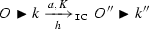
(Immediate causes LTS) The immediate causes LTS (LTS\(_{\mathtt {IC}}\)) is the smallest LTS on minimal P-processes generated by the following rule

This rule replaces the continuation with its minimal version and, in order to keep track of the original identity of events, equips the transition with a “history map”, mapping canonical events to the original ones. In particular, the one with image \(1\) is the fresh event generated by the original transition. Notice that the continuation poset may contain non-maximal events, for instance
with \(2 \prec _O 1\) cannot be further reduced.
The notion of bisimilarity for LTS\(_{\mathtt {IC}}\) is more involved: while, given two P-processes, we may find a common poset for them (if any), which enables them to be compared w.r.t. \(\sim _{\mathtt {PO}}\), this is not possible in LTS\(_{\mathtt {IC}}\), because its states must have minimal posets. In other words: posets have a meaning local to states. Therefore, we have to introduce an explicit correspondence between posets.
Definition 13
(Immediate causes bisimilarity) An immediate causes bisimulation \(R\) is a set of triples \((O \blacktriangleright k,\sigma ,O' \blacktriangleright k')\) such that \(\sigma \) is a partial monotone bijection from \(O\) and \(O'\) and:
-
(i)
if
 then \(\sigma \) is defined on \(K\), and there are
  and \(\sigma '\) such that \((O'' \blacktriangleright k'', \sigma ',O''' \blacktriangleright k''') \in R\) and \(\sigma '(n) = m\) implies \(h(n) = h'(m) = 1\) or \(\sigma (h(n)-1) = h'(m) - 1\);
 -
(ii)
if
 then \(\sigma \) is defined on \(K\), and there are
  and \(\sigma '\) as in the previous item.
 then
then  and
and  then
then  and
and The greatest such bisimulation is denoted \(\sim _{\mathtt {IC}}\). We write \(O \blacktriangleright k \sim _{\mathtt {IC}}^\sigma O' \blacktriangleright k'\) to mean \((O \blacktriangleright k,\sigma , O' \blacktriangleright k') \in \sim _{\mathtt {IC}}\).
Notice that states should be able to simulate each other only up to \(\sigma \). The continuations are again related by a partial bijection \(\sigma '\) between \(O''\) and \(O'''\), which should act consistently on names by “commuting” with history maps \(h, h'\) and \(\sigma \). In the case \(h(n) \ne 1 \ne h'(m)\), since \(h\) and \(h'\) have codomain \(\delta _K(O')\) and \(\delta _{\sigma (K)}(O'')\) respectively, where names in \(O\) and \(O'\) have been shifted by one, we should subtract one in order to recover the counterparts of \(h(n)\) and \(h(m)\) in \(O\) and \(O'\).
We have the following correspondence between \(\sim _{\mathtt {IC}}\) and \(\sim _{\mathtt {PO}}\).
Theorem 2
\(\sim _{\mathtt {IC}}\) is fully abstract w.r.t. \(\sim _{\mathtt {PO}}\) in the following sense:
-
(i)
If \(O \rhd k\sim _{\mathtt {PO}}O \rhd k'\) then \([\![O \rhd k ]\!] \sim _{\mathtt {IC}}[\![O \rhd k' ]\!]\);
-
(ii)
If \(O \blacktriangleright k\sim _{\mathtt {IC}}^\sigma O' \blacktriangleright k'\) then for all \(\hat{O}\rhd \hat{k}\) and \(\hat{O}\rhd \hat{k}'\) such that:
-
(a)
\([\![\hat{O}\rhd \hat{k} ]\!] = O \blacktriangleright k\) and \([\![\hat{O}\rhd \hat{k}' ]\!] = O' \blacktriangleright k'\);
-
(b)
\(\mu _{\hat{O}\rhd \hat{k}}|_{dom(\sigma )} = \mu _{\hat{O}\rhd \hat{k}'} \circ \sigma \);
we have \(\hat{O} \rhd \hat{k}\sim _{\mathtt {PO}}\hat{O} \rhd \hat{k}'\).
-
(a)
Remark 1
The transition system LTS\(_{\mathtt {IC}}\) is derived in a similar way as Montanari and Pistore causal automata. However, their derivation removes causal relations from states, keeping only the underlying set of events. This also affects the notion of bisimulation, where partial bijections are between sets of names. We have chosen to keep causal relations, and to give a compatible notion of bisimulation. This seems a natural choice, and it reflects what will produced, in a completely automatic and standard way, by our categorical construction.
5 Coalgebraic semantics
In this section we construct a coalgebra for causal semantics, equivalent to LTS\(_{\mathtt {PO}}\). Since we work in a more abstract setting, we do not need to concretely represent events as natural numbers to implement event generation. The notions introduced in the previous section are instances of our categorical machinery.
Definition 14
(Categories \(\mathbf {FinPos},\mathbf {P}\) and \({\mathbf {P}_{m}}\)) Let \(\mathbf {FinPos}\) be the category of finite posets and monotone functions, and let \(\mathbf {P}\) its skeletal category, i.e., a full subcategory of \(\mathbf {FinPos}\) such that each object is isomorphic to one of \(\mathbf {FinPos}\), but no two distinct objects are isomorphic. The category \({\mathbf {P}_{m}}\) is the subcategory of \(\mathbf {P}\) with only injective and poset-reflecting morphisms.
We recall that for locally finitely presentable categories, such as \(\mathbf {FinPos}\), a skeletal category can always be constructed. The category \(\mathbf {P}\) can be seen as a full subcategory of \(\mathbf {Graph}\), the category of graphs and graph homomorphisms. Its objects are isomorphism class representatives of a particular class of graphs, namely directed acyclic graphs with all reflexive and transitive edges. Its subcategory \({\mathbf {P}_{m}}\) will be our index category for presheaves. We now describe its structure.
Proposition 4
The category \({\mathbf {P}_{m}}\) is small and has pullbacks, computed as in \(\mathbf {Graph}\).
The category \({\mathbf {P}_{m}}\) lacks colimits, but the ones we are interested in can be computed in \(\mathbf {P}\). We will be more precise when presenting such colimits.
We introduce some notation for particular objects and morphisms of \({\mathbf {P}_{m}}\): we denote by \([k]\) the discrete poset with \(k\) elements and by \([k]^\top \) the same poset plus a top element; \(b_k :[k] \rightarrow [k]^\top \) is the embedding of \([k]\) into \([k]^\top \) picking its bottom elements; and \(\top _k :[1] \rightarrow [k]^\top \) picks the top element in \([k]^\top \).
In \(\mathbf {P}\) we can model the operator \(\delta _{K}\) of Definition 9 as a pushout. Given \(O \in |\mathbf {P}|\), let \(K :[k] \hookrightarrow O\) be the subobject in \({\mathbf {P}_{m}}\) picking \(K\) within \(O\). Then we have

Explicitly, \(\delta _K (O)\) is constructed as follows: the disjoint union of \(O\) and \([k]^\top \) is made, and then the bottom elements of \([k]^\top \) and the causes \(K\) are identified, resulting in \(O\) plus a fresh top event for \(K\); the transitive closure of this relation gives \(\delta _K (O)\). Notice that, since \(K\) reflects posets, causes of the fresh event must be incomparable, i.e., maximal events in \(O\). This agrees with Definition 9.
For instance, let \(\{e_1,e_2\}\) be the discrete poset \([2]\). Then \(\delta _{\{e_1,e_2\}}([2])\) is given by
Lemma 1
The diagram (5) is a square in \({\mathbf {P}_{m}}\).
We remark that (5) is not a pushout in \({\mathbf {P}_{m}}\), but we are not interested in its mediating morphisms.
Now we want to turn \(\delta _K\) into an endofunctor on \({\mathbf {P}_{m}}\). However, \(\delta _K\) does not define a proper functor, because \(K\) depends on the specific poset fed to \(\delta _K\). Therefore, we make \(\delta \) independent from \(K\) by adding a new event for each possible set of independent causes, i.e., each discrete subposet of \(O\).
This idea is formalized as follows. Let \(K^k_1 , \ldots , K^k_{n_k} :[k] \hookrightarrow O\) be all subposets of \(O\) with \(k\) elements. Notice that, by (4), the image of each \(K^k_i\) must be a discrete poset, in other words: \(K^k_i\) only picks events that are not already related. Suppose \(O\) has cardinality \(o\). Then all the spans  , namely those involved in (5), can be combined in the following colimit in \(\mathbf {P}\)

Given a morphism \(\sigma :O \rightarrow O'\), let \(\sigma ^\star :O^* \rightarrow O'^\star \) be the corresponding morphism induced by the universal property of the above colimit. It can be easily verified that if \(\sigma \) is a morphism of \({\mathbf {P}_{m}}\) then so is \(\sigma ^\star \). Roughly, \(\sigma ^\star \) acts as \(\sigma \) on old elements in \(O^\star \), i.e., those in the image of \(old_O\), and maps injectively each fresh top event for a set of causes \(K\) to the top event for \(K\sigma \), preserving and reflecting the new causal relations involving that event. Therefore we can define the following allocation endofunctor \(\delta :{\mathbf {P}_{m}}\rightarrow {\mathbf {P}_{m}}\)
For instance, \(\delta ([2])\) is given by
Remark 2
Our allocation operator \(\delta \) may seem inefficient: it generates a new event for each possible set of causes, but only one of them will appear in the continuation after a transition. However, having a functor on \({\mathbf {P}_{m}}\) allows us to lift it to presheaves in a way that ensures the existence of both left and right adjoint (giving Kan extensions along \(\delta \)) for the lifted functor, and then preservation of both limits and colimits, which is essential for coalgebras employing such functor. Generation of unused events is not really an issue: as we will see later, it is always possible to recover the support of a process, i.e., the poset formed by events actually appearing in it.
Now we look at the category \(\mathbf {Set}^{\mathbf {P}_{m}}\) of presheaves on posets. Since \({\mathbf {P}_{m}}\) is small it follows that \(\mathbf {Set}^{\mathbf {P}_{m}}\) is locally finitely presentable and has all limits and colimits, in particular products and coproducts. The following constructs are relevant for us.
Presheaf of event names. \(\mathcal {E}:{\mathbf {P}_{m}}\rightarrow \mathbf {Set}\) gives the set of event names occurring in \(O \in |{\mathbf {P}_{m}}|\); formally:
Explicitly, \(\mathcal {E}\) sends \(O \in |{\mathbf {P}_{m}}|\) to \({\mathbf {P}_{m}}[[1],O]\), which is isomorphic to \(|O|\), and \(\sigma :O \rightarrow O'\) in \({\mathbf {P}_{m}}\) to the function \(\lambda e \in {\mathbf {P}_{m}}[[1],O].\sigma \circ e\), which renames the event \(e\) according to \(\sigma \).
Finite powerset. \(\fancyscript{P}_f:\mathbf {Set}^{\mathbf {P}_{m}}\rightarrow \mathbf {Set}^{\mathbf {P}_{m}}\), defined as \(\mathcal {P}_f \circ (-)\), where \(\mathcal {P}_f\) is the finite powerset on \(\mathbf {Set}\).
Event allocation operator. \(\varDelta :\mathbf {Set}^{\mathbf {P}_{m}}\rightarrow \mathbf {Set}^{\mathbf {P}_{m}}\), given by \((-) \circ \delta \). Explicitly, for \(P :{\mathbf {P}_{m}}\rightarrow \mathbf {Set}\) and \(O \in |{\mathbf {P}_{m}}|\), \(\varDelta P (O) = P( \delta (O) )\). Intuitively, it generates processes with additional fresh events.
Presheaf of labels. \(\mathcal {L}:{\mathbf {P}_{m}}\rightarrow \mathbf {Set}\) given by
For each \(O \in |{\mathbf {P}_{m}}|\), this functor gives pairs \((a,K)\) of an action \(a\) and a set of causes \(K\), selected among events in \(O\).
We use these operators to define our behavioral endofunctor.
Definition 15
(Behavioral functor) The behavioral functor \(B :\mathbf {Set}^{\mathbf {P}_{m}}\rightarrow \mathbf {Set}^{\mathbf {P}_{m}}\) is
To understand this definition, consider a \(B\)-coalgebra \((P,\rho )\). Given \(O \in |{\mathbf {P}_{m}}|\) and \(p \in P(O)\), \(\rho _O(p)\) is a finite set of triples \((a,K,p')\), telling that \(p'\) is the continuation of \(p\) after observing \(a,K\). The continuation always belongs to \(\varDelta P (O)\), i.e., to \(P(\delta (O))\), because every transition allocates a new event.
The category \({B}\mathbf{-Coalg }\) is well-behaved: it has a final \(B\)-coalgebra, and the behavioral equivalence it induces coincides with \(B\)-bisimilarity. This is thanks to the following properties.
Proposition 5
\(B\) is accessible and covers pullbacks.
\(B\)-coalgebras can be regarded as particular LTSs whose states are elements of presheaves, i.e., pairs \(O \rhd p\).
Definition 16
(\({\mathbf {P}_{m}}\)-ILTS) A \({\mathbf {P}_{m}}\)
-indexed labelled transition system (\({\mathbf {P}_{m}}\)-ILTS) is a pair  of a presheaf \(P :{\mathbf {P}_{m}}\rightarrow \mathbf {Set}\) and a finitely-branching transition relation
  of the form:

such that, for each morphism \(\sigma :O \rightarrow O'\) in \({\mathbf {P}_{m}}\):
-
(i)
if
 then
then  (transitions are preserved by \(\sigma \));
 -
(ii)
if
 then there are \(l'\) and \(\delta (O) \rhd p''\) such that \(l'[\sigma ] = l\), \(p''[\delta \sigma ] = p'\) and
  (transitions are reflected by \(\sigma \));
 then
then  (transitions are preserved by
  then there are
  (transitions are reflected by
 Proposition 6
\({\mathbf {P}_{m}}\)-ILTSs are in bijection with \(B\)-coalgebras.
The natural notion of bisimulation for these transition systems is \({\mathbf {P}_{m}}\) -indexed bisimulation.
Definition 17
(\({\mathbf {P}_{m}}\)
-indexed bisimulation) A \({\mathbf {P}_{m}}\)
-indexed bisimulation on a \({\mathbf {P}_{m}}\)-ILTS  is an indexed family of relations \(\{ R_O \subseteq P(O) \times P(O) \}_{O \in |{\mathbf {P}_{m}}|}\) such that, for all \((p,q) \in R_O\)
-
(i)
if
 then there is \(O' \rhd q'\) such that
  and \((p',q') \in R_{O'}\);
 -
(ii)
for all \(\sigma :O \rightarrow O'\), \((p[\sigma ],q[\sigma ]) \in R_{O'}\).
 then there is
  and
and This definition closely resembles that of poset-indexed causal bisimulation (Definition 10). We have an additional condition (ii), requiring closure under morphisms of \({\mathbf {P}_{m}}\). This is not satisfied by all poset-indexed causal bisimulation, but it holds for the greatest one (Theorem 1).
We have the following correspondence.
Proposition 7
Let \((P,\rho )\) be a \(B\)-coalgebra. Then \(B\)-bisimulations on \((P,\rho )\) are in bijection with \({\mathbf {P}_{m}}\)-indexed bisimulations on the induced \({\mathbf {P}_{m}}\)-ILTS.
Notice that, unlike Aczel-Mendel bisimulations, a \(B\)-bisimulation (namely, a Hermida-Jacobs one) needs not be the carrier of a \(B\)-coalgebra in order to be a bisimulation. This strong requirement is the reason why some \({\mathbf {P}_{m}}\)-indexed bisimulations cannot be turned into Aczel-Mendler ones (see [17, 3.3, Anomaly]).
We now show that LTS\(_{\mathtt {PO}}\) can be represented as a \({\mathbf {P}_{m}}\)-ILTS. We form a presheaf from states of LTS\(_{\mathtt {PO}}\) as follows.
Definition 18
(Presheaf of P-processes) The presheaf of P-processes \(\fancyscript{C}:{\mathbf {P}_{m}}\rightarrow \mathbf {Set}\) is given by
The action of \(\fancyscript{C}\) on morphisms needs to apply the closure operator, after renaming the process: this guarantees that the result is a proper P-process. Notice that elements of \(\fancyscript{C}\) are defined over events with an abstract identity, which may not be natural numbers. More precisely, we implicitly assume the following translation from states of LTS\(_{\mathtt {PO}}\). For each finite poset \(O\) over natural numbers, take the isomorphism \(\varphi _O :O \rightarrow [O]\) within \(\mathbf {FinPos}\), where \([O]\) is the object of \({\mathbf {P}_{m}}\) canonically representing the isomorphism class of \(O\). Then \([O] \rhd k\varphi \) gives the proper element of \(\fancyscript{C}\) corresponding to \(O \rhd k\).
We have the following property.
Lemma 2
\(\fancyscript{C}\) preserves pullbacks.
We are ready to translate LTS\(_{\mathtt {PO}}\) to a \({\mathbf {P}_{m}}\)-ILTS.
Definition 19
(Poset \({\mathbf {P}_{m}}\)-ILTS\(_{\mathtt {PO}}\)) The Poset \({\mathbf {P}_{m}}\)-ILTS (\({\mathbf {P}_{m}}\)-ILTS\(_{\mathtt {PO}}\)) is the smallest one generated by the rule

The rule in this definition computes a casual process with poset \(\delta (O)\) from \(O' \rhd k'\). This is done by replacing \(1\), the concrete fresh event in \(k'\), with the abstract fresh event associated to \(K\) in \(\delta (O)\), via the corresponding colimit map. All the other events are renamed accordingly. This definition gives a proper \({\mathbf {P}_{m}}\)-ILTS: transitions are clearly of the required form, and preservation and reflection of transition follows from analogous properties of LTS\(_{\mathtt {PO}}\) (Proposition 3).
We call causal coalgebra the \(B\)-coalgebra equivalent to \(({\fancyscript{C},\Longrightarrow }_\mathtt{PO})\). We have the following theorem, which collects the results of this section, instantiated to the causal coalgebra.
Theorem 3
\({\mathbf {P}_{m}}\)-indexed bisimulations on \(({\fancyscript{C},\Longrightarrow }_\mathtt{PO})\) are equivalent to:
-
\(B\)-bisimulations on the causal coalgebra;
-
poset-indexed causal bisimulations closed under injective and poset-reflecting renamings.
In particular, we have that the greatest \({\mathbf {P}_{m}}\)-indexed bisimulation, \(B\)-bisimilarity on the causal coalgebra and \(\sim _{\mathtt {PO}}\) are all equivalent, thanks to Theorem 1. These, by Proposition 5, are equivalent to the kernel of the unique morphism from the causal coalgebra to the final one.
Remark 3
The carrier of the final \(B\)-coalgebra can be intuitively described as follows. It is a presheaf whose elements are pairs \(O \rhd T\) of a poset and a tree \(T\). When \(O \rhd T\) is the image of a P-process \(O \rhd k\) via the final morphism, then \(T\) is similar to a (strong) causal tree for \(k\), but its edges only exhibit the most recent events. The “missing information”, i.e., the full history of events, is provided by \(O\).
6 From coalgebras to HD-automata
In order to give a characterization of the causal coalgebra in terms of named sets, we employ the results of [7]. Here authors define a symmetry group over a category \(\mathbf {C}\) to be a collection of morphisms in \(\mathbf {C}[c,c]\), for any \(c \in |\mathbf {C}|\), which is a group w.r.t. composition of morphisms. Then they take families of such groups as their notion of generalized named sets. A first result establishes the equivalence between these families and coproducts of symmetrized representables, that are functors of the form
where \(\varPhi _i\) is a symmetry group over \(\mathbf {C}\) with domain \(c_i\), and the quotient identifies morphisms that are obtained one from the other by precomposing elements of \(\varPhi _i\). These functors, in turn, are shown to be isomorphic to wide-pullback-preserving presheaves on \(\mathbf {C}\), a wide pullback being the limit of a diagram with an arbitrary number of morphisms pointing to the same object (pullbacks are a special case, with two such morphisms). The following theorem summarizes the described results.
Theorem 4
Let \(\mathbf {C}\) be a category that is small, has wide pullbacks, and such that all its morphisms are monic and those in \(\mathbf {C}[c,c]\) are isomorphisms, for every \(c \in |\mathbf {C}|\). Then every wide-pullback-preserving \(P \! \in \!|\mathbf {Set}^\mathbf {C}|\) is equivalent to a coproduct of symmetrized representables.
Our category \({\mathbf {P}_{m}}\) satisfies the hypothesis of this theorem: it is small and has wide pullbacks due to the existence of pullbacks. In fact, the diagram of a wide pullback in \({\mathbf {P}_{m}}\) is formed by a finite number of morphisms, because a finite poset always has a finite number of ingoing poset-reflecting monomorphisms, so its limit can be computed via binary pullbacks. Moreover, \({\mathbf {P}_{m}}\) has only monos, by definition, and \({\mathbf {P}_{m}}[O,O]\) clearly has only isomorphisms, for each \(O \in |{\mathbf {P}_{m}}|\). Finally, our presheaf of processes \(\fancyscript{C}\) preserves (wide) pullbacks, so there exists an equivalent coproduct of symmetrized representables.
Theorem 4 indeed describes an equivalence between pullback-preserving presheaves and families, which induces one on coalgebras. We shall now investigate this point. Let \(\mathbf {Set}^{\mathbf {P}_{m}}_{\diamond }\) be the full subcategory of \(\mathbf {Set}^{\mathbf {P}_{m}}\) formed by pullback-preserving presheaves. We have that our behavioral endofunctor \(B\) indeed defines an endofunctor on \(\mathbf {Set}^{\mathbf {P}_{m}}_{\diamond }\).
Proposition 8
All the endofunctors on \(\mathbf {Set}^{\mathbf {P}_{m}}\) in Definition 15 can be restricted to endofunctors on \(\mathbf {Set}^{\mathbf {P}_{m}}_{\diamond }\).
Let \(B_\diamond :\mathbf {Set}^{\mathbf {P}_{m}}_{\diamond }\rightarrow \mathbf {Set}^{\mathbf {P}_{m}}_{\diamond }\) be the restricted behavioral endofunctor. The causal coalgebra is clearly a \(B_\diamond \)-coalgebra. Restricting to \(\mathbf {Set}^{\mathbf {P}_{m}}_{\diamond }\) does not affect the final coalgebra: \({B}\mathbf{-Coalg }\) and \({B_\diamond }\mathbf{-Coalg }\) have the same final object and final morphisms from common objects. In fact, the terminal sequence starts from the final presheaf \(1\), pointwise defined as the singleton set, which trivially preserves pullbacks, and goes through \(B^n(1) = B_\diamond ^n(1)\), for any \(n\).
Corollary 1
(of Theorem 4) Let \(\widetilde{B}\) the behavioral endofunctor on families defined by lifting all functors in Definition 15 along the equivalence. Then the category \({B_\diamond }\mathbf{-Coalg }\) is equivalent to \({\widetilde{B}}\mathbf{-Coalg }\).
In particular, the equivalence relates the final \(B_\diamond \)-coalgebra and the final \(\widetilde{B}\)-coalgebra, and their final morphisms. Moreover, since kernels are preserved by equivalence, identifications made by the final morphisms are preserved, hence behavioral equivalence is preserved too. A concrete, automata-theoretic characterization of \(\widetilde{B}\) has been provided in simpler cases (see [8, 15]). Our case is more complex and we leave its treatment for future work.
Now that we have proved that our categorical setting is suitable for HD-automata, we can translate the causal coalgebra to a HD-automaton. We work in a more concrete setting: we introduce a notion of named set closer to a more traditional one, but indeed equivalent to the families mentioned above. Given a set \(S\) of morphism and a morphism \(\sigma \) in \({\mathbf {P}_{m}}\), we write \(S \circ \sigma \) for the set \(\{ \tau \circ \sigma \mid \tau \in S \}\) (analogously for \(\sigma \circ S\)).
Definition 20
Let \(\mathbf{{Sym} }({\mathbf {P}_{m}})\) be the category defined as follows:
-
objects are sets \(\varPhi \subseteq {\mathbf {P}_{m}}[O,O]\) that are groups w.r.t. composition in \({\mathbf {P}_{m}}\);
-
morphisms \(\varPhi _1 \rightarrow \varPhi _2\) are sets of morphisms \(\sigma \circ \varPhi _1\) such that \(\sigma :dom(\varPhi _1) \rightarrow dom(\varPhi _2)\) and \(\varPhi _2 \circ \sigma \subseteq \sigma \circ \varPhi _1\).
Definition 21
The category \({\mathbf {P}_{m}}\mathbf{-Set }\) is defined as follows:
-
objects are \({\mathbf {P}_{m}}\) -named sets, that are pairs \(N = (Q_N,\mathtt {G}_N)\) of a set \(Q_N\) and a function \(\mathtt {G}_N :Q \rightarrow |Sym({\mathbf {P}_{m}})|\). The local poset of \(q \in Q_N\), denoted \(\Vert q \Vert \), is \(dom(\sigma )\), for any \(\sigma \in \mathtt {G}_N(q)\).
-
morphisms \(f :N \rightarrow M\) are \({\mathbf {P}_{m}}\) -named functions, that are pairs \(( h , \varSigma )\) of a function \(h :Q_N \rightarrow Q_M\) and a function \(\varSigma \) mapping each \(q \in Q_N\) to a morphism \(\mathtt {G}_M(h(q)) \rightarrow \mathtt {G}_N(q)\) in \(Sym({\mathbf {P}_{m}})\).
In the rest of this section we give an explicit description of the \({\mathbf {P}_{m}}\)-named set produced from \(\fancyscript{C}\) by the equivalence. Its elements will be minimal P-processes: we will show that the translation from P-processes to minimal ones is achieved via categorical constructions. We need the notions of support, seed and orbit.
Definition 22
(Support and seed) Given \(O \rhd k\), its support, denoted \(supp(k)\), is the wide-pullback-object of the following morphisms
Let \(\varSigma _{k}\) be the embedding \(supp(k) \hookrightarrow O\) given by the pullback. Then the seed of \(k\), denoted \(seed(k)\), is the unique element of \(\fancyscript{C}(supp(k))\) such that \(seed(k)[\varSigma _{k}] = k\).
As shown in [7, 12], preservation of pullbacks is essential to ensure existence and uniqueness of seeds. The seed operation achieves the first two properties of minimal P-processes (see Definition 11): \(seed(k)\) just contains immediate causes for each of its components and \(supp(O)\) contains all and only those causes. This is illustrated by the following example.
Example 2
Consider the following P-process
where \(O\) is a poset over \(\{1,2,3,4\}\) with
Then the set of morphisms of Definition 22 has two elements \(f_1 :O_1 \rightarrow O\) and \(f_2 :O_2 \rightarrow O\) where \(O_1\) is a poset over \(\{1,2,3\}\) with \(2 \prec _{O_1} 1\) and \(3 \prec _{O_1} 1\), and \(O_2\) is a poset over \(\{1,2\}\) such that \(2 \prec _{O_2} 1\). These morphisms just map events preserving their names. We have

It is easy to check that the pullback object of \(f_1\) and \(f_2\) is \(O_2\), so the corresponding seed is \(O_2 \rhd \{1,2\} \mathbin {\Rightarrow }p_1 \parallel \{2\} \mathbin {\Rightarrow }p_2\). Notice that the event \(4\) has been discarded, because it does not syntactically appear in the process, but also \(3\), because it is not an immediate cause for either \(p_1\) or \(p_2\).
Definition 23
(Orbit) The orbit of \(O \rhd k\) is
We denote by \([k]^o\) a canonical choice of an element of \(orb(k)\).
The orbit of \(k\) is the set of elements obtained by applying to it all functions induced by poset automorphisms. The representative \([k]^o\) plays the same role as \([O \rhd k]_{\cong }\) defined in the previous section. However, each \(\cong \)-equivalence class may contain P-processes with different, but isomorphic, posets. These posets all become the same one in \({\mathbf {P}_{m}}\), due to skeletality, so it is enough to consider automorphisms, which are always iso in \({\mathbf {P}_{m}}\).
Definition 24
The \({\mathbf {P}_{m}}\)-named set of minimal P-processes is \((C,\mathtt {G}_C)\), where
Let us explain this definition. The set \(C\) is produced from elements of \(\fancyscript{C}\): for each of these, we compute the seed, and then we only take the canonical representative for the seed’s orbit. The former operation achieves the third requirement for minimal P-processes. The symmetry group for a process is the set of poset automorphisms fixing the process.
The HD-automaton on \((C,\mathtt {G}_C)\) in \({\widetilde{B}}\mathbf{-Coalg }\), equivalent to the causal coalgebra, is the category-theoretic counterpart of LTS\(_{\mathtt {IC}}\): states are minimal P-processes, and transitions have history maps. In \({\widetilde{B}}\mathbf{-Coalg }\), history maps come from the fact that coalgebra structure maps are \({\mathbf {P}_{m}}\)-named functions, so they are equipped with backward morphisms towards the poset of the source state. However, there is a crucial difference: states of the HD-automaton have symmetries, which allow for further identifications of states. For instance, the process
can be associated the symmetry \(\{id_{[2]},(1 \ 2),(1 \ 2)^{-1}\}\), because swapping \(1\) and \(2\) yields bisimilar processes.
7 Conclusions
In this paper we have given a construction for obtaining compact models of causal semantics. In order to do this, we have equipped causal processes with nominal structures, namely posets over event names, representing causal relations. We have presented a first, set-theoretic version of our construction, along the lines of [14], and then a category-theoretic one that employs standard constructs and results for nominal calculi, namely presheaf-based coalgebras and their equivalence with HD-automata. The categorical version is much more concise and natural. In particular, reducing the state-space and showing that this operation preserves the semantics require some technical effort in the set-theoretic version, whereas the categorical version employs a general construction that automatically performs this reduction in a semantics-preserving way.
This paper is mainly related to [14]. While the definition of causal automata should be attributed to the ingenuity of their authors, the derivation of HD-automata we show in this paper is due to a general categorical construction. The main difference between the two notions of automata is in the information each state keeps: causal automata keep events, but discard their causal relations; our HD-automata retain causal relations, in the form of posets, and, in addition, there are symmetry groups over them. This allows for a further reduction of states. How this difference affects bisimulations has yet to be investigated.
A representation of events in terms of names, with the aim of capturing Darondeau–Degano causal semantics, can also be found in [5], even if in the different context of tile systems. We can cite [6] for the introduction of transitions systems for causality whose states are elements of presheaves, intended to model the causal semantics of the \(\pi \)-calculus as defined in [4]. However, the index of a state is a set of names, without any information about events and causal relations. The advantage of our index category is that it allows reducing the state-space in an automatic way, exploiting a standard categorical construction. This cannot be done in the framework of [6]. Finally, an HD-automaton for causality has been described in [8], but it is derived as a direct translation of causal automata and its states do not take into account causal relations.
Other related works are [19, 20], where event structures have been characterized as (contravariant) presheaves on posets. While the meaning of presheaves is similar, the context is different: we consider the more concrete realm of process algebras, coalgebras and nominal automata. A more precise correspondence with such models should be worked out.
References
Adámek, J.: Introduction to coalgebra. Theory Appl. Categ. 14(8), 157–199 (2005)
Adámek, J., Bonchi, F., Hülsbusch, M., König, B., Milius, S., Silva, A.: A coalgebraic perspective on minimization and determinization. In: FoSSaCS, pp. 58–73 (2012)
Adámek, J., Rosický, J.: Locally Presentable and Accessible Categories. Cambridge University Press, Cambridge (1994)
Boreale, M., Sangiorgi, D.: A fully abstract semantics for causality in the \(\pi \)-calculus. Acta Inf. 35(5), 353–400 (1998)
Bruni, R., Montanari, U.: Dynamic connectors for concurrency. Theor. Comput. Sci. 281(1–2), 131–176 (2002)
Cattani, G.L., Sewell, P.: Models for name-passing processes: interleaving and causal. Inf. Comput. 190(2), 136–178 (2004)
Ciancia, V., Kurz, A., Montanari, U.: Families of symmetries as efficient models of resource binding. Electr. Notes Theor. Comput. Sci. 264(2), 63–81 (2010)
Ciancia, V., Montanari, U.: Symmetries, local names and dynamic (de)-allocation of names. Inf. Comput. 208(12), 1349–1367 (2010)
Darondeau, P., Degano, P.: Causal trees: Interleaving + causality. In: Semantics of Systems of Concurrent Processes, pp. 239–255 (1990)
Ferrari, G.L., Montanari, U., Tuosto, E.: Coalgebraic minimization of HD-automata for the \(\pi \)-calculus using polymorphic types. Theor. Comput. Sci. 331(2–3), 325–365 (2005)
Fiore, M.P, Turi, D.: Semantics of name and value passing. In: LICS, pp. 93–104 (2001)
Gadducci, F., Miculan, M., Montanari, U.: About permutation algebras, (pre)sheaves and named sets. Higher-Order Symb. Comput. 19(2–3), 283–304 (2006)
Kanellakis, P.C., Smolka, S.A.: Ccs expressions, finite state processes, and three problems of equivalence. Inf. Comput. 86(1), 43–68 (1990)
Montanari, U., Pistore, M.: Minimal transition systems for history-preserving bisimulation. In: STACS, pp. 413–425 (1997)
Montanari, U., Pistore, M.: Structured coalgebras and minimal HD-automata for the \(\pi \)-calculus. Theor. Comput. Sci. 340(3), 539–576 (2005)
Rutten, J.J.M.M.: Universal coalgebra: a theory of systems. Theor. Comput. Sci. 249(1), 3–80 (2000)
Staton, S.: Name-Passing Process Calculi: Operational Models and Structural Operational Semantics. Technical Report 688, University of Cambridge (2007)
Staton, S.: Relating coalgebraic notions of bisimulation. Logical Methods Comput. Sci. 7(1), 1–21 (2011)
Staton, S., Winskel, G.: On the expressivity of symmetry in event structures. In: LICS, pp. 392–401 (2010)
Winskel, G.: Event structures as presheaves—two representation theorems. In: CONCUR, pp. 541–556 (1999)
Worrell, J.: Terminal sequences for accessible endofunctors. Electr. Notes Theor. Comput. Sci. 19, 24–38 (1999)
Acknowledgments
The research for this paper has been partially funded by the EU Integrated Project 257414 ASCENS and by the Italian MIUR Project CINA (PRIN 2010), Grant Number 2010LHT4KM. We are very grateful to Sam Staton for his clarifications about Hermida Jacobs bisimulations. We thank the anonymous reviewers for their useful comments and suggestions.
Author information
Authors and Affiliations
Corresponding author
Appendix: Proofs
Appendix: Proofs
Proof
(of Proposition 2)
-
\((\Longrightarrow )\) We prove that the following relation is a causal bisimulation
$$\begin{aligned} R = \{ (k,k') \mid \exists O :O \rhd k\sim _{\mathtt {PO}}O \rhd k' \} \end{aligned}$$Suppose \(O \rhd k\xrightarrow {a,K}_{\mathtt {PO}} O' \rhd k''\) and the simulating transition is \(O \rhd k' \xrightarrow {a,K}_{\mathtt {PO}} O' \rhd k'''\). Then we can recover simulating transitions in LTS\(_{\mathtt {DD}}\) as follows
$$\begin{aligned} k\xrightarrow {a,{{K\,}\!\!\downarrow _{O}}}_{\mathtt {DD}} k'' \qquad k' \xrightarrow {a,{{K\,}\!\!\downarrow _{O}}}_{\mathtt {DD}} k''' \end{aligned}$$where \({{}\!\!\downarrow _{}}\) is extended to sets of causes by performing their closure. Since \(O' \rhd k'' \sim _{\mathtt {PO}}O' \rhd k'''\), we have \((k'',k''') \in R\).
-
\((\Longleftarrow )\) We prove that the following relation is a poset-indexed causal bisimulation
$$\begin{aligned} R_O = \{ (O \rhd k,O \rhd k') \mid k\sim _{\mathtt {DD}}k' \} \end{aligned}$$Suppose \(k\xrightarrow {a,K}_{\mathtt {DD}} k''\) and \(k' \xrightarrow {a,K}_{\mathtt {DD}} k'''\). Then the rule in Definition 9, applied to both transitions, gives transitions in LTS\(_{\mathtt {PO}}\) with the same label, and the same source and target posets. If the the target poset is \(\delta _M(O)\), then from \(k'' \sim _{\mathtt {DD}}k'''\) it follows \((\delta _M(O) \rhd k'', \delta _M(O) \rhd k''') \in R_{\delta _M(O)}\).\(\square \)
Proof
(of Proposition 3) We show (i), the other point is analogous. We rely on the following properties of LTS\(_{\mathtt {DD}}\), which can be easily checked by induction on the inference via rules Fig. 1: for all \(O \rhd k\), \(\sigma :O \rightarrow O'\) injective and poset-reflecting, and \(O''\) such that \(O\) is a subposet of \(O''\), we have
Property (7) is the least obvious: the idea is that, since labels of LTS\(_{\mathtt {DD}}\) show the whole history of causes for an action, the additional ones in \(O''\), preceding those in \(K\), should be shown as well; the continuation is closed accordingly.
Now, take \(O \rhd k\xrightarrow {a,K}_{\mathtt {PO}} \delta _K(O) \rhd k'\) and \(\sigma :O \rightarrow O'\) injective and poset-reflecting. By the rule in Definition 9 there is a transition in LTS\(_{\mathtt {DD}}\)
If we apply (6) and then (7) to this transition, we get
Observe that
The first equation holds because \({{}\!\!\downarrow _{O'}}\) only adds to \(K'\sigma \) events that are smaller w.r.t. \(\prec _{O'}\). The second equation holds because \(\sigma \) is poset-reflecting: this prevents some maximal, thus unrelated, events in \(K'\) to become non-maximal in \(K'\sigma \) due to additional causal relations involving them in \(O'\).
From (9) it follows
where the first equation comes from transitivity: adding causal relations from \(1\) to \(K'\sigma \) and its past causes in \(O'\) is equivalent to adding relations to only maximal events in \(K'\sigma \), because transitivity will take care of adding the missing ones.
We conclude by applying (10) to the continuation of (8), which becomes of the required form, and then the rule of Definition 9 to infer the required transition. The computation of the maximal causes yields the desired result, thanks to (9). \(\square \)
In order to prove Theorem 2, we need the following lemmata, whose proofs are straightforward.
Lemma 3
For each \(O \rhd k\), \(\mu _{O \rhd k}\) is injective and poset-reflecting.
Lemma 4
Let \([\![O \rhd k ]\!] = O' \rhd k'\), then \({{(k'\mu _{O \rhd k})}\!\!\downarrow _{O}} = k\).
An immediate consequence is the following one.
Lemma 5
 is generated by \(O \rhd k\xrightarrow {a,K}_{\mathtt {PO}} \delta _K(O) \rhd {{(k'h)}\!\!\downarrow _{\delta _K(O)}}\) via the rule in Definition 12.
Proof
(of Theorem 2)
Item (i). We prove that the following relation is an immediate causes bisimulation
We only show how the derivation of a simulating transition for one of \([\![O \rhd k ]\!]\). The symmetric case is analogous. Let \([\![O \rhd k ]\!] = \tilde{O}\blacktriangleright \tilde{k}\), and suppose it has the following transition

Then, by Lemma 5, we have
Now, let \(\mu _1 = \mu _{O \rhd k}\): by Lemma 3, we can apply Proposition 3(i) to the last transition and get
where \({{(\tilde{k}\mu _1)}\!\!\downarrow _{O}} = k\) is due to Lemma 4. Therefore we have \([\![\delta _{K\mu _1}(O) \rhd \tilde{k}_3 ]\!] = \tilde{O}' \blacktriangleright \tilde{k}_1\), and the associated map \(\tilde{O}' \rightarrow \delta _{K\mu _1}(O)\) is given by composing those applied to the continuations of (12) and (13), namely
Suppose (13) can be simulated by \(O \rhd k'\) as follows
Let \([\![O \rhd k' ]\!] = \tilde{O}'' \blacktriangleright \tilde{k}'\) and \(\mu _2 = \mu _{O \rhd k'}\). Then, by Lemma 3, we can apply Proposition 3(ii) to (15) and \(\mu _2\), obtaining
such that \(\tilde{K}\mu _2 = K \mu _1\) and \({{(\tilde{k}'' {\mu _2}^{\!+})}\!\!\downarrow _{\delta _{K\mu _1}(O)}} = k''\). Let \(h' = \mu _{\delta _{\tilde{K}}(\tilde{O}'') \rhd \tilde{k}''}\). Applying the rule of Definition 12 to (16) we get

It is not difficult to check that \([\![\delta _{\tilde{K}}(\tilde{O}'') \rhd \tilde{k}'' ]\!] = [\![\delta _{K\mu _1}(O) \rhd k'' ]\!]\): the intuition is that taking immediate causes from \(O \rhd k'\), then adding a new event, and taking again immediate causes, has the same result as adding the event straight away and then taking immediate causes. Therefore \(\mu _{\delta _{K\mu _1}(O) \rhd k''}\) can be expressed as composition of the maps from the continuation of (17) to that of (16), and from the latter to that of (15), namely
Now we shall check that (11) and (17) are actually simulating transitions. From \(\tilde{K}\mu _2 = K \mu _1\) and the definition of \(\sigma \) (recall that \(\mu _1 = \mu _{O \rhd k}\) and \(\mu _2 = \mu _{O \rhd k'}\)) it follows \(\tilde{K}= K \sigma \). Let \(\sigma '\) be defined by
The right equation is equivalent to \(\mu _{\delta _{K\mu _1}(O) \rhd k''}(n) = \mu _{\delta _{K\mu _1}(O) \rhd \tilde{k}_3}(m)\), by (14) and (18), so \(([\![\delta _{K\mu _1}(O) \rhd k'' ]\!],\sigma ',[\![\delta _{K\mu _1}(O) \rhd \tilde{k}_3 ]\!]) \in R\). It remains to check that it is a proper bisimulation triple. Take \(n,m\) such that \(\sigma '(n) = m\). We have
where the first and last implication follow from the definition of \({\mu _1}^{\!+}\) and \({\mu _2}^{\!+}\). For \(h(n),h(m) > 1\), expanding the definition of \({\mu _1}^{\!+}\) and \({\mu _2}^{\!+}\) we get \(\mu _1(h(n)-1) = \mu _2(h'(m)-1)\), hence \(\sigma (h(n)-1) = h'(m)-1\), by the definition of \(R\).
Item (ii).We prove that the following family of relations is a poset-indexed causal bisimulation
To ease notation, let \(\mu _1 = \mu _{\hat{O}\rhd \hat{k}}\) and \(\mu _2 = \mu _{\hat{O}\rhd \hat{k}'}\). We only show that each transition of \(\hat{O}\rhd \hat{k}\) can be simulated by one of \(\hat{O}\rhd \hat{k}'\). The proof for the symmetric statement is analogous. Suppose \(\hat{O}\rhd \hat{k}\) has the following transition
Then, by Proposition 3(ii) and Lemma 3, we can rename it via \(\mu _1\) and get
where \(\tilde{K}\mu _1 = K\). Applying the rule in Definition 12, we get

Now, suppose that this transition can be simulated by \(O' \blacktriangleright k'\) as follows

and \([\![ \delta _{\tilde{K}}(O) \rhd \tilde{k}' ]\!] \sim _{\mathtt {IC}}^\sigma O'' \blacktriangleright k''\). Applying Lemma 5 we get
and then, from Proposition 3(i) with renaming \(\mu _2\), and applying Lemma 4 to the resulting source process, we get
From hypothesis (ii.b) and \(\tilde{K}\subseteq dom(\sigma )\), by definition of \(\sim _{\mathtt {IC}}^\sigma \), we have \((\tilde{K}\sigma ) \mu _2 = \tilde{K}\mu _1 = K\), so (19) and (20) have the same label, and we must have \(\delta _{(\tilde{K}\sigma )\mu _2}(O') = \delta _{K}(\hat{O})\). Finally, we have to check (ii.a) and (ii.b) on continuations:
-
(ii.a)
We have \([\![ \delta _{\tilde{K}}(O) \rhd \tilde{k}' ]\!] = [\![\delta _K(\hat{O}) \rhd \hat{k}'' ]\!]\) and \([\![\delta _K(\hat{O}) \rhd \tilde{k}'' ]\!] = O'' \blacktriangleright k''\), as already explained in Item (i) for analogous transitions;
-
(ii.b)
Let \(\tilde{\mu }_1 = \mu _{\delta _{\tilde{K}}(O) \rhd \tilde{k}'}\) and \(\tilde{\mu }_2 = \mu _{\delta _K(\hat{O}) \rhd \tilde{k}''}\). We have to check \(\tilde{\mu }_1|_{dom(\sigma ')} = \tilde{\mu }_2 \circ \sigma '\). Take \(n \in dom(\sigma ')\). Then, by the equivalence between continuations exhibited in the proof of (ii.a), we have \(\tilde{\mu }_1 = {\mu _1}^{\!+} \circ h\) and \(\tilde{\mu }_2 = {\mu _2}^{\!+} \circ h'\), so
$$\begin{aligned} \tilde{\mu }_1(n) = \tilde{\mu }_2(\sigma '(n))&\iff {\mu _1}^{\!+}(h(n)) = {\mu _2}^{\!+}({h'(\sigma '(n))}) \end{aligned}$$We have two cases, by the property relating \(\sigma '\) with \(h,h'\) and \(\sigma \):
-
\(h(n) = h'(\sigma (n)) = 1\), then \({\mu _1}^{\!+}(h(n)) = 1 ={\mu _2}^{\!+}({h'(\sigma '(n))})\);
-
\(h(n), h'(\sigma (n)) > 1\), then \(\sigma (h(n)-1) =h'(\sigma '(n)) - 1\), and so
$$\begin{aligned}&\mu _2(\sigma (h(n) - 1)) = \mu _2(h'(\sigma '(n)) - 1) \quad \text{(applying }\, \mu _2 \text{ on } \text{ both } \text{ sides) } \\&\iff \qquad \!\! \mu _1(h(n)-1) \!=\!\mu _2(h'(\sigma '(n)) \!-\! 1) \quad (\hbox {by hypothesis } \mu _1(n) = \mu _2(\sigma (n))) \\&\iff \qquad \!\! {\mu _1}^{\!+}(h(n)) \!=\! {\mu _2}^{\!+}({h'(\sigma '(n))}) \quad \text{(by } \text{ definition } \text{ of }\,{\mu _1}^{\!+}\,\text{ and }\, {\mu _2}^{\!+},\\&\qquad \qquad \qquad \qquad \qquad \qquad \qquad \qquad \qquad \qquad \quad \,\hbox {adding}\, 1\, \text{ to } \text{ both } \text{ members) } \end{aligned}$$
-
\(\square \)
We need the following lemma in order to prove Proposition 4.
Lemma 6
Let \(f,g,h\) morphisms of \(\mathbf {P}\) such that \(f = h \circ g\). If \(f\) and \(h\) are injective and poset-reflecting then so is \(g\).
Proof
Suppose \(f :O_1 \rightarrow O_3\), \(g :O_1 \rightarrow O_2\) and \(h :O_2 \rightarrow O_3\). Injectivity of \(g\) is straightforward to prove. As for poset-reflection, suppose \(g\) does not preserve posets, namely there are \(x,y \in |O_1|\) such that \(x \not \prec _{O_1} y\) and \(g(x) \prec _{O_2} g(y)\). Then \(h(g(x)) \prec _{O_3} h(g(y))\), because \(h\) preserves posets, therefore \(f(x) \prec _{O_3} f(y)\), but then \(f\) does not preserve posets, a contradiction. \(\square \)
Proof
(of Proposition 4) Smallness comes from the same property of \(\mathbf {P}\). We now show that pullbacks exists and are computed as in \(\mathbf {Graph}\). Consider the following pullback in \(\mathbf {Graph}\)

where \(\sigma _1,\sigma _2,q_1,q_2\) are morphisms in \({\mathbf {P}_{m}}\). We have to show that \(O \in |{\mathbf {P}_{m}}|\) and \(p_1,p_2,m\) are morphisms in \({\mathbf {P}_{m}}\). That \(O \in |{\mathbf {P}_{m}}|\), namely it is a dag with reflexive and transitive edges, follows from analogous properties of \(O_1,O_2\) and \(O_3\) and the fact that \(O\) has an edge iff each graph among \(O_1,O_2\) and \(O_3\) has a corresponding edge picked by the pullback morphisms, by definition of pullback in \(\mathbf {Graph}\). From this last observation also follows that \(p_1\) and \(p_2\) preserve posets. They are also injective, because monos are stable under pullbacks, so they belong to \({\mathbf {P}_{m}}\). As for \(m\), it belongs to \({\mathbf {P}_{m}}\) by Lemma 6 applied to the commutative triangle (1). \(\square \)
We need some technical lemmata in order to prove Lemma 1. We fix the following span in \({\mathbf {P}_{m}}\)

Lemma 7
Consider the following pushout in \(\mathbf {Graph}\)

Then:
-
(i)
\(p_1\) and \(p_2\) are injective and preserve posets;
-
(ii)
\(G\) satisfies antisymmetry and reflexivity.
Proof
-
(i)
Injectivity follows from the fact that monomorphisms in \(\mathbf {Graph}\) are stable under pushouts. Suppose \(p_1\) does not reflect posets (the case of \(p_2\) is identical). Then there are \(x,y \in |O_1|\) such that \(x \not \prec _{O_1} y\) and \(p_1(x) \prec _{G} p_1(y)\). But then, by definition of pushout in \(\mathbf {Graph}\), we must have \(x',y' \in |O|\) such that \(\sigma _1(x') = x\), \(\sigma _1(y') = y\) and \(\sigma _2(x') \prec _{O_2} \sigma _2(y')\) (otherwise \(p_1(x) \not \prec _{G} p_1(y)\)). Since \(\sigma _2\) reflects posets, we must have \(x' \prec _O y'\), but then \(\sigma _1\) does not reflect posets, a contradiction.
-
(ii)
Reflexivity follows from self-loops of \(O_1\) and \(O_2\) being preserved by \(p_1\) and \(p_2\). Suppose antisymmetry does not hold, namely there are \(x,y \in |G|\), such that \(x \prec _G y\), \(y \prec _G x\) and \(x \ne y\). Then, since \(p_1\) and \(p_2\) reflect posets by (i), we can only have two cases:
-
\(x \prec _G y\) and \(y \prec _G x\), with \(x \ne y\), are images of edges in \(O_i\) via \(p_i\) (\(i \in \{1,2\}\)): then \(O_i\) would not satisfy the antisymmetric property, a contradiction;
-
\(x \prec _G y\) and \(y \prec _G x\) are images of one edge \(x_1 \prec _{O_1} y_1\) in \(O_1\) and one \(y_2 \prec _{O_2} x_2\) in \(O_2\) via \(p_1\) and \(p_2\) respectively, with \(x_i \ne y_i\): then there must be \(x',y' \in |O|\), with \(x' \ne y'\), such that \(\sigma _i(x') = x_i\) and \(\sigma _i(y') = y_i\); but then \(x' \prec _O y'\) and \(y' \prec _O x'\), because \(\sigma _1\) and \(\sigma _2\) reflect posets, i.e., \(O\) does not satisfy the antisymmetric property, a contradiction.
-
\(\square \)
Lemma 8
If the square on the left is a pushout in \(\mathbf {Graph}\) then the one on the right is a pushout in \(\mathbf {P}\) and a square in \({\mathbf {P}_{m}}\)

where \(G^+\) is the transitive closure of \(G\) and \(cl = G \hookrightarrow G^+\).
Proof
Transitive closure defines a functor \(\mathbf {Graph}\rightarrow \mathbf {Cat}\), where \(\mathbf {Cat}\) is the category of small categories, left adjoint to the functor sending a category to its underlying graph, therefore it preserves pushouts. It is easy to see that \(\mathbf {P}\) is equivalent to a full subcategory of \(\mathbf {Cat}\), and that the left pushout is sent to a pushout in this subcategory, corresponding to the right square. In fact, transitive closure does not affect  , by idempotency, and Lemma 7(ii) says that \(G^+\) is indeed an object of \(\mathbf {P}\). The right square is indeed a pushout: mediating morphisms towards objects in \(\mathbf {P}\) correspond, along the equivalence, to those in \(\mathbf {Cat}\).
Finally, in order to show that the right square is in \({\mathbf {P}_{m}}\), we have to prove that \(cl \circ p_1\) and \(cl \circ p_2\) are injective and reflect posets. Injectivity follows from Lemma 7(i) and injectivity of \(cl\). By Lemma 7(ii) we know that \(p_1\) and \(p_2\) reflect posets. Suppose \(cl \circ p_1\) does not (\(cl \circ p_2\) is treated analogously). Then there are \(x,y \in |O_1|\), with \(x \ne y\), such that \(x \not \prec _{O_1} y\) and \(cl(p_1(x)) \prec _{G^+} cl(p_1(y))\). We have two cases:
-
\(cl(p_1(x)) \prec _{G^+} cl(p_1(y))\) is added by the transitive closure. Then there is \(z \in |G|\) such that \(p_1(x) \prec _G z \prec _G p_1(y)\). If \(z\) is the image via \(p_1\) of some \(z' \in |O_1|\), since \(p_1\) reflects posets we must have \(x \prec _{O_1} z' \prec _{O_1} y\), but \(x \not \prec _{O_1} y\) by assumption, which is absurd because \(O_1\) would not be transitively closed. If \(z' = p_2(z)\) then, by definition of pushout, we must have \(x',y' \in |O_2|\) sent by \(p_2\) to \(p_1(x)\) and \(p_1(y)\), respectively. Since \(p_2\) reflects posets, we must have \(x' \prec _{O_2} z' \prec _{O_2} y'\) and \(x' \not \prec _{O_2} y'\), by \(p_1(x) \not \prec _G p_1(y)\), but then \(O_2\) is not transitively closed, a contradiction.
-
\(p_1(x) \prec _G p_1(y)\). Then \(p_1\) would not reflect posets.
\(\square \)
Proof
(of Lemma 1) This is just a corollary of Lemma 8. \(\square \)
Proof
(of Proposition 5) For accessibility: \(\fancyscript{P}_f\) is known to be accessible; \(\mathcal {L}\) is accessible, because it can be regarded as a constant endofunctor on \(\mathbf {Set}^{\mathbf {P}_{m}}\); \(\varDelta \) is accessible, because it has a right adjoint, namely the functor computing right Kan extensions along \(\delta \). The thesis follows from accessibility being preserved by composition and products.
In order to show that \(B\) covers pullbacks, we will show that it has the form \(\fancyscript{P}_f\circ B'\), with \(B'\) a pullback preserving endofunctor on \(\mathbf {Set}^{\mathbf {P}_{m}}\). The thesis will follow from \(\fancyscript{P}_f\) covering pullbacks (see [18]). \(\varDelta \) has a left adjoint, namely the functor computing left Kan extensions along \(\delta \), then it preserves pullbacks; \(\mathcal {L}\) can be seen as a constant, hence pullback-preserving, endofunctor on \(\mathbf {Set}^{\mathbf {P}_{m}}\). \(B'\) is the product of these two functors, so it preserves pullbacks. \(\square \)
Proof
(of Proposition 6) The transition relation can be turned into a natural transformation in \(\mathbf {Set}^{\mathbf {P}_{m}}\): (i) and (ii) guarantee that such relation obeys the naturality condition. The other direction clearly holds. \(\square \)
Proof
(of Proposition 7) Requirement (ii) of Definition 17 corresponds to the fact that a \(B\)-bisimulation \(R\) is a functor with action on \(\sigma \) given by \((p,q) \mapsto (p[\sigma ],q[\sigma ])\). Requirement (i) corresponds to the fact that \(RO\) is “almost” an ordinary bisimulation, because computing \(\overline{B}R(O)\) essentially amounts to computing \(\overline{B_{flts}}(RO)\) (see Sect. 2.2) for each \(O \in |{\mathbf {P}_{m}}|\), as images in \(\mathbf {Set}^{\mathbf {P}_{m}}\) are computed pointwise in \(\mathbf {Set}\), with the difference that continuations are not in \(RO\), but in \(R(\delta O)\). \(\square \)
Proof
(of Proposition 8) Let \(P\) be a pullback-preserving presheaf. It is well-known that the finite powerset \(\mathcal {P}_f\) in \(\mathbf {Set}\) preserves pullbacks of monos, thus so does \(\mathcal {P}_f \circ P\).
The presheaf of label can be seen as an endofunctor on \(\mathbf {Set}^{\mathbf {P}_{m}}\) with constant action \(\mathcal {L}\), so we have to show that \(\mathcal {L}\) preserves pullbacks: it is obtained by combining, via product and composition, the covariant hom functor \(\mathcal {E}\), which is known to preserve pullbacks, the finite powerset and the constant presheaf \(Act \cup \{\tau \}\), which trivially preserves pullbacks; therefore \(\mathcal {L}\) preserves pullbacks.
The interesting case is \(\varDelta \). We have to show that \(\delta \) preserves pullbacks, which implies that \(P \circ \delta \), i.e., \(\varDelta P\), has the same property. Consider the following squares in \({\mathbf {P}_{m}}\), where the left one is a pullback

The left diagram can be embedded into the right one using \(old\) maps. This gives the action of the right diagram’s morphisms on elements that are not generated by \(\delta \), and tells that the right diagram indeed behaves like a pullback on such elements. Now, consider any element added by \(\delta \) to \(O\). This is the top element for a set of incomparable events \(K \subseteq |O|\). Since pullbacks are constructed as in \(\mathbf {Graph}\) (Proposition 4), \(K\) is incomparable in \(O\) if and only if \(p_1(K)\) and \(p_2(K)\) are incomparable in \(O_1\) and \(O_2\), respectively, and have the same image in \(O_3\), again formed by incomparable events. By definition of the action of \(\delta \) on morphisms, \(\delta (p_i)\) maps the fresh top element for \(K\) to the ones for \(p_i(K)\) (\(i=1,2\)), and these are mapped by \(\delta (\sigma _1)\) and \(\delta (\sigma _2)\) to the same one in \(\delta (O_3)\). Therefore \(\delta (O)\) is indeed a pullback object, with pullback maps \(\delta (p_1)\) and \(\delta (p_2)\). \(\square \)
Rights and permissions
About this article

Cite this article
Bruni, R., Montanari, U. & Sammartino, M. Revisiting causality, coalgebraically. Acta Informatica 52, 5–33 (2015). https://doi.org/10.1007/s00236-014-0207-9
Received:
Accepted:
Published:
Issue Date:
DOI: https://doi.org/10.1007/s00236-014-0207-9