Multi-objective shape optimization of a hydraulic turbine runner using efficiency, strength and weight criteria

Abstract

An approach for multi-discipline automatic optimization of the hydraulic turbine runner shape is presented. The approach accounts hydraulic efficiency, mechanical strength and the weight of the runner. In order to effectively control the strength and weight of the runner, a new parameterization of the blade thickness function is suggested. Turbine efficiency is evaluated through numerical solution of Reynolds-averaged Navier-Stokes equations, while the finite element method is used to evaluate the von Mises stress in the runner. An objective function, being the weighted sum of maximal stress and the blade volume, is suggested to account for both the strength and weight of the runner. Multi-objective genetic algorithm is used to solve the optimization problem. The suggested approach has been applied to automatic design of a Francis turbine runner. Series of three-objective optimization runs have been carried out. The obtained results clearly indicate that simultaneous account of stress and weight objectives accompanied by thickness variation allows obtaining high efficiency, light and durable turbine runners.

1 Introduction

Multidisciplinary design optimization techniques become more and more applied in the field of turbomachinery due to the rapid development of high-performance computers, numerical methods and multi-objective optimization algorithms. It offers the capability of automated design of complex three-dimensional shapes of flow passages of fans, compressors, pumps and turbines, satisfying a number of multi-physics objectives. In the case of hydraulic turbines these objectives formulate the hydrodynamic, structural, and economical requirements to the shape of the flow passage.

The runner is the most complex and the most unique part of the Francis hydraulic turbine, Fig. 1. It is specially designed for any new project. Runner geometry determines the power of the turbine, its efficiency, durability and safety of operation. The runner operates in a variety of regimes, experiencing strong static and dynamic loadings and cavitation. That’s why at the stage of turbine design the greatest attention is paid to the runner.

Fig. 1

Francis hydraulic turbine (up) and its runner (down)

The main requirements to the runner geometry are:

• high efficiency in a wide, prescribed range of operating points;

• the absence or at least minimal amount of cavitation, aimed to minimize cavitation erosion;

• limited static and dynamic stresses to avoid unit destruction and ensure reliable operation through years.

Therefore, the runner design is inherently a complex multi-objective multiple operating point optimization problem.

There are number of publications devoted to the development and application of automatic design and optimization tools, based on CFD analysis of the fluid flow in turbine flow passage, see (Cherny et al. 2008, Kurosawa and Nakamura 2009, Flores et al. 2012) among others. The general problem statement is to find the runner geometry providing the best performance with some geometrical and cavitational constraints. Earlier papers considered one-operating point efficiency maximization, while the later, such as (Enomoto et al. 2012; Lyutov et al. 2015), suggested multiple operating point optimization techniques. Commonly, the hydraulic performance is being evaluated in frames of the steady state Reynolds-averaged Navier-Stokes (RANS) equations. Usually runner geometry is defined by the values of 20–40 free parameters, and evolutionary algorithm is used to guide the search for the optimal solution. Approximate (surrogate) models are frequently used to accelerate the convergence of the genetic algorithm (Marjavaara and Lundström 2007; Georgopoulou et al. 2008; Risberg et al. 2008).

Structural analysis has been incorporated first into the design process of aerodynamic turbomachines, such as fans, compressors, and wind turbines. Pierret et al. (2007) considered automatic shape optimization of a compressor blade using fluid and structural analysis. At that the aerodynamic computations have been performed in three operating points. The optimization was guided by genetic algorithm assisted by a surrogate model. Successful coupled aerodynamic and structural optimization of a transonic fan has been performed by Joly et al. (2014). These authors emphasized the importance of thickness variation for providing the strength of the rotor blades.

The first reference regarding the fluid and structural optimization of the hydraulic turbine runner was the conference paper of Mazzouji et al. (2004). There the structural analysis of the runner was performed using the simplified shell-model approach, avoiding the solution of elasticity equations in the blade volume. Risberg et al. (2008) also considered fluid flow and mechanical optimization of the Francis turbine runner. During the optimization the structural analysis was performed using the finite-element method (FEM). In (Bannikov et al. 2010) we suggested the runner shape optimization technique that accounts for both hydraulic efficiency of the whole turbine and the runner strength. Von Mises stress was used as the strength objective function. However, in that paper the stress analysis was performed for isolated blade, firmly mounted to the runner crown. Moreover, blade fillets were not taken into account.

Stadler and Celic (2015) performed a coupled fluid and structural optimization of a guide vane profile of a pump-turbine. Both static and dynamic stresses as well as guide vane efficiency were accounted as constraints in that paper. The guide vane volume was the objective. It was able to obtain thinner but durable guide vane profiles. Moreover, the obtained optimal solutions with thinner profiles were also superior in terms of hydraulic efficiency.

Considering the runner geometry optimization the cost of the runner manufacturing is an additional objective that should to be taken into account. At present the cost of the Francis runner is nearly proportional to its metal consumption, or simply to its weight. At that the blades give about one half the total runner weight. Therefore the lighter the blades the cheaper the runner. Another advantage of the light runner is a reduced axial thrust, which is beneficial for mechanical design of the bearings and of the entire unit. Note that the weight reduction is now a common objective in the area of wind turbine optimization, see for example (Wang et al. 2011), (Liao et al. 2012), (Hu et al. 2016). However, in the field of hydraulic turbines this issue has not been addressed before.

The strength and weight properties of the runner are effectively controlled by distribution of the blade thickness. Besides this, blade thickness affects efficiency and cavitation characteristics of the runner. Indeed, the thinner the blade the smaller the drag, and hence, the higher the efficiency of the turbine near the best efficiency operating point (BEP). From the other hand, thin leading edges are prone to flow separation and leading edge cavitation at non-optimal attack angles. Therefore thickness distribution needs to be varied, especially if we want to account strength and weight objectives during the process of runner optimization. Different approaches for parameterization of blade thickness distribution are discussed in (Ferrando 2005).

Recently we suggested an approach for automatic optimization of Francis (Cherny et al. 2008; Lyutov et al. 2015) and Kaplan (Semenova et al. 2014) runners and their draft tubes. In (Lyutov et al. 2015) the runner shape was parameterized by 24 design parameters, while 9 design parameters were used for the draft tube. Although thickness distribution was kept constant, this approach proved to be very effective for improvement of the whole turbine performance.

The present paper advances the above approach and suggests:

• a novel parameterization of the blade thickness function;

• a new objective function, taking into account both maximal stress in the runner and its weight (metal consumption);

• a problem statement and an approach to multi-criteria optimization of Francis turbine runner shape, allowing to simultaneously increase the hydraulic efficiency of the turbine in a wide range of operating points, as well as reduce maximal stresses and weight of the runner.

The paper is organized as follows. Section 2 describes the parameterization of the blade thickness distribution. Section 3 briefly outlines the optimization workflow based on multi-objective genetic algorithm. Governing equations, boundary conditions, and numerical algorithm for fluid flow simulations are discussed in Section 4. Section 5 describes the finite element approach for mechanical evaluation of the runner geometries. A new objective functional, accounting for both runner stress and runner weight is given Section 6. The developed optimization methodology is applied for the design of Francis turbine runner from a real rehabilitation project. Three distinct three-objective optimizations are performed in Sections 7, 8 in order to demonstrate the capabilities of the presented optimization approach and the advantages of thickness variation in providing efficient, light and durable runner blade geometries.

2 Parameterization of thickness distribution

Francis turbine runner consists of crown, band and a number of blades, as shown in Fig. 1. For the task of optimization the runner shape is represented by the set of its geometrical parameters x = (x₁, …, x_n). Parameterization of the median blade surface (16 free parameters), meridian projections of leading edge (LE), trailing edge (TE), band and crown (8 free parameters, see Fig. 2) is described in (Lyutov et al. 2015). Let us consider in detail the parameterization of the blade thickness function.

Fig. 2

Variation of median (RZ) projection of Francis runner

The surface of the runner blade consists of а pressure side and а suction side that can be defined in the following way:

$$ \left\{\begin{array}{l}\kern0.5em {\mathbf{r}}_{\mathrm{p}}\left(t,s\right)={\mathbf{r}}_{\mathrm{m}}\left(t,s\right)+d\left(t,s\right)\cdot \mathbf{n}\left(t,s\right)\\ {}\kern0.5em {\mathbf{r}}_{\mathrm{s}}\left(t,s\right)={\mathbf{r}}_{\mathrm{m}}\left(t,s\right)-d\left(t,s\right)\cdot \mathbf{n}\left(t,s\right)\end{array}\right. $$

Here

t ∈ [0, t_max] and s ∈ [0, s_max]:

are the natural parameters of the median surface, Fig. 3;

r_m(t, s):

is the radius-vector of the median surface;

r_p(t, s)and r_s(t, s):

are the radius-vectors of pressure and suction sides, respectively;

d(t, s):

is the thickness function, see Fig. 4;

n(t, s):

is the unit normal to the median surface, pointed out towards the pressure side.

Fig. 3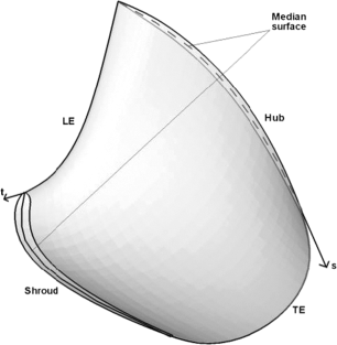

(t,s)-parameterization of median blade surface

Fig. 4

Thickness function d(t,s)

Let d₀(t,s) be the thickness function of the initial blade. Define s_m(t) as a position of the maximal thickness for given t, Fig. 5. Let d_m(t) = d(t,  s_m(t)) be the maximal thickness of the blade profile for given t. It is assumed that s_m(t) and d_m(t) are the quadratic functions of t. Thickness variation is implemented through variation of the following 6 parameters, defining the shape of s_m(t)and d_m(t), see Fig. 5:

• s_m1 = s_m(0), s_m2 = s_m(t_max/2), s_m3 = s_m(t_max) are the positions of maximum thickness in the crown, in the middle, and in the band sections, respectively;

• d_m1 = d_m(0), d_m2 = d_m(t_max/2), d_m3 = d_m(t_max) are the maximum thicknesses in the crown, in the middle, and in the band sections, respectively.

Fig. 5

Parameterization of thickness distribution

In the final step the modified thickness function d(t, s) is constructed for each t by scaling the blade profiles of the initial blade d₀(t, s) to fit the new position s_m(t) and the value of maximal thickness d_m(t).

3 Optimization strategy

Assuming that for every runner geometry x = (x₁, …, x_n) the corresponding objective functions F_i(x) can be evaluated, the task of runner optimization can be formulated as follows. Find the vector of parameters x^∗, providing the minimum values of all the objective functions. Since the problem is multi-objective, the solution is not a unique point x^∗, but a Pareto set. For finding Pareto set we utilize multi-objective genetic algorithm (MOGA), based on the works of Fonseca and Fleming (1993) and Horn and Nafpliotis (1993). The algorithm is described in (Cherny et al. 2008). In the present paper the real-coded version of MOGA is used. No surrogate models were used to accelerate the convergence of MOGA. In order to reduce the optimization time, evaluation of the objective functions for different individuals within the population is parallelized using MPI. Each individual is computed at its own processor of the computational cluster.

The optimization workflow is shown in Fig. 6. The following actions are automatically performed for every modification of runner geometry.

• 1. Reconstruction of the runner surface.

• 2. Generation of finite volume mesh for CFD analysis.

• 3. CFD analysis for each considered operating point.

• 4. Generation of finite element mesh for FEM analysis.

• 5. Interpolation of pressure field, computed in step 3, onto the surface nodes of FEM mesh.

• 6. Computation of stress-strain field in the runner (FEM analysis).

• 7. Evaluation of the objective functions: efficiency, stress, cavitation, etc.

Fig. 6

Schematic workflow of runner optimization

Typically, 30–60 generations of about 100 individuals need to be computed to obtain virtually converged Pareto front.

4 Fluid flow analysis

During the automatic optimization the CFD analysis of each runner geometry is performed in order to evaluate its efficiency and cavitation characteristics. For that the 3D flow-field in turbine flow passage is computed in frames of steady state incompressible Reynolds-averaged Navier-Stokes (RANS) equations:

$$ {\displaystyle \begin{array}{l}\frac{\partial {u}_1}{\partial {x}_1}+\frac{\partial {u}_2}{\partial {x}_2}+\frac{\partial {u}_3}{\partial {x}_3}=0,\\ {}\sum \limits_{j=1}^3\frac{\partial \left({u}_i{u}_j\right)}{\partial {x}_j}+\frac{\partial \widehat{p}}{\partial {x}_i}=\sum \limits_{j=1}^3\frac{\partial }{\partial {x}_j}\left[{v}_{eff}\left(\frac{\partial {u}_i}{\partial {x}_j}+\frac{\partial {u}_j}{\partial {x}_i}\right)\right]+{f}_i,\kern1.5em i=1,\kern0.5em 2,\kern0.5em 3,\end{array}} $$

(1)

where (u₁, u₂, u₃) is the velocity vector, $\widehat{p}=p/\rho +2k/3$, p is the pressure, ρ is the density. Stationary reference frame is used for static domains (wicket gate channel and draft tube), while the rotating reference frame is used for the runner. Thus, f₁ = x₁ω² + 2v₂ω, f₂ = x₂ω² + 2v₁ω, f₃ = g, g = 9.81 m²/s, where ω is the angular velocity of runner rotating around the x₃ axis, while ω = 0 for the wicket gate and the DT. The standard k − ε eddy-viscosity model with log-law wall functions is used for the turbulence closure. This model provides a good balance between computational robustness and accuracy of efficiency evaluation.

For the solution of RANS equations an in-house CFD solver described in (Cherny et al. 2006a, b) is used. Pressure and velocity fields are linked together using artificial compressibility approach (Rogers et al. 1991). In this approach the solution of steady state RANS (1) is sought as the limit of time-dependent solution of unsteady RANS equations, modified by adding time derivative of pressure into continuity equation. The modified unsteady RANS equations are discretized using implicit finite-volume scheme. Spatial accuracy of the scheme is determined by the accuracy of flux evaluation through the faces of mesh cells. Third order accurate MUSCL scheme is used for evaluation of inviscid fluxes, while 2nd order central difference scheme is used for evaluation of viscous fluxes. The use of time-implicit discretization leads to a large system of non-linear discrete equations at every time level. Since only steady state solution of the discrete equations is of interest, non-linear system of discrete equations is linearized and approximately LU-factorized. Thus the solution at the next time level is efficiently obtained using two sweeps of computational domain. In the case of structured mesh forward sweep is done in the direction of increasing cell indexes (i, j, k), while backward sweep is done in the opposite direction.

Computational domain consists of one wicket gate (WG) channel, one runner channel and the whole draft tube, Fig. 7. This approach, called periodic stage approach, assumes that the flow-fields in all the WG channels, as well as in all the runner channels are the same. The use of periodic stage approach with rotating runner domain requires special treatment of “wicket gate – runner” and “runner – draft tube” interfaces. The present paper employs commonly used “mixing plane” approach, consisted in circumferential averaging of flow parameters (p, V_r, V_z, V_u, k, ε) before passing them from one domain to another. Here V_r, V_z, V_u are the radial, axial, and circumferential components of the velocity field.

Fig. 7

Computational domain and mesh for CFD analysis

Constant total flow energy and constant flow angle are specified in the WG inlet, while hydrostatic pressure distribution is specified in the outlet cross section (Panov et al. 2012). With this statement of boundary conditions the discharge is found as a part of the solution.

A block structured mesh employed for the computations is shown in Fig. 7. The mesh consists of about 57,000 cells for WG domain, 68,000 cells for runner domain, and 100,000 cells for the DT. The benefit of using the hexahedral mesh is the higher solution accuracy especially near the boundary layers. An example of pressure distribution in the runner obtained in the computations is shown in Fig. 8. This pressure field is subsequently applied as a boundary condition for mechanical computation.

Fig. 8

Computed pressure contours in the runner domain

Efficiency of the turbine is evaluated from the formula

$$ \eta =\frac{M\omega}{\rho gQH}{\eta}_{mech}{\eta}_{vol} $$

(2)

where M is the computed hydrodynamic torque acting on the runner, Q is the computed discharge, Н is the given turbine head, η_mech is the mechanical efficiency accounting disk friction losses; η_vol is the volumetric efficiency taking into account flow leakage. Note, that η_mech and η_vol are close to unity and can be assumed constant for the case of runner optimization.

In order to demonstrate the capabilities of CFD code, Fig. 9 shows the comparison of turbine efficiency, computed and measured experimentally for turbine of specific speed ${n}_q={nQ}^{0.5}/{H}^{0.75}=72$. Four computational meshes are used in Fig. 9: mesh1 (~97.000 cells in total), mesh2 (~225,000 cells), mesh3 (~316,000 cells), and mesh4 (~1060,000 cells). Mesh3 is 1.5 times finer in all spatial directions than mesh1, mesh4 is 1.5 times finer than mesh3. Mesh2 is similar to that, shown in Fig. 7. It can be seen that the value of efficiency gradually increases with mesh refinement. However the computed results are in good agreement with experimental data even for the coarse mesh. Starting from mesh2, CFD computations predict the efficiency with a good level of accuracy (~0.4%), which is comparable to the error of efficiency measurements on the test rig (±0.2%). From this analysis mesh2 is taken for optimizations in Sec. 7, providing a good level of prediction accuracy at reasonable computational efforts.

Fig. 9

Efficiency versus discharge: mesh refinement study

Cavitation is another important characteristic of turbine flow. Thorough approach for evaluation of cavitation characteristic requires series of two-phase flow simulations for different values of Thoma number (Panov et al. 2012). However this approach is laborious to implement within the optimization loop. In frames of single-phase incompressible Navier-Stokes (1) the cavitation characteristic can be approximately estimated through the analysis of size and position of cavitation zone, the area on suction side of the runner blade, where pressure drops below the vapor pressure. In order to quantify the amount of cavitation, a relative area of cavitation zone A_cav = S_cav/S_suc is computed for each runner modification. During the optimization A_cav can be used as a constraint or objective function.

5 Structural analysis

During the operation the runner is subject to hydrodynamic, gravity, and centrifugal forces. Since periodic runner approach is assumed in frames of CFD analysis, the mechanical analysis is also performed in frames of the periodic approach. One runner blade, complemented with a crown sector and a band sector, is computed, Fig. 10. Finite element mesh in the solid body, automatically generated for FEM analysis is also shown in the figure. The stresses are usually concentrated in the blade near the crown and the band. In the process of runner manufacturing the attachments of the blade to crown and band surfaces are rounded by welded fillets. The fillets dramatically reduce the stresses in the runner. Therefore it is necessary to account for the fillets at the stage of stress computation. Figure 11 is the close view of the finite element mesh near the crown, showing the fillets.

Fig. 10

Mesh and boundary conditions for FEM analysis

Fig. 11

Blade fillets at the crown

Evaluation of static stress distribution is found in frames of linear elasticity equations using finite element method from Ansys package v14.0. Boundary conditions are the following. Pressure field obtained as the result of CFD computation is applied to the blade and to the internal surfaces of crown and band. Zero pressure is set at the outer surfaces of crown and band. Rigid attachment (zero displacements) is set at the surface where the runner is connected to the shaft. Cyclic periodicity condition is applied at periodic boundaries.

The estimation of runner strength is based on the von Mises stress σ, evaluated as

$$ \sigma =0.5\sqrt{{\left({\sigma}_{11}-{\sigma}_{22}\right)}^2+{\left({\sigma}_{22}-{\sigma}_{33}\right)}^2+{\left({\sigma}_{33}-{\sigma}_{11}\right)}^2+\left({\sigma}_{12}^2+{\sigma}_{23}^2+{\sigma}_{31}^2\right)} $$

where σ_ij are the components of the stress tensor. At the stage of runner design it is necessary to provide that maximal von Mises stress σ_max = max(σ) meets the condition

$$ {\sigma}_{\mathrm{max}}\le {\alpha \sigma}_{\mathrm{c}}. $$

(3)

Here σ_с is the yield stress of the steel and α < 1 is the required safety factor. Typically, α~0.3. Inequality (3) can serve as a mechanical constraint for optimization. However, in the present paper the stress is accounted as an objective function to be minimized. The stress objective function is the ratio of the maximum stress of the given runner modification to the maximum stress of the initial one,

$$ {S}_2=\frac{\sigma_{\mathrm{max}}}{{\left({\sigma}_{\mathrm{max}}\right)}_{initial}}. $$

(4)

Considerations behind taking the stress as one of the objective functions (instead of using a simple constraint (3)) are the following. During the operation, the stress field in the runner consists of static part and dynamic part. Dynamic stresses are the result of unsteady flow phenomena, caused by rotor-stator interaction, vortex rope rotation and so on. Frequency and amplitude of these pulsating stresses determine the lifetime of the runner, and thus, are of great importance for turbine designers. However, accurate computation of the dynamic stresses requires unsteady CFD simulation of the flow field. One of the approaches used in practice, estimates the value of the dynamic stresses as a certain fraction of the static stress, σ_dyn ≃ a ⋅ σ_static, where a is an empirical constant. Therefore minimization of static stress should reduce the dynamic part as well.

6 New stress-weight functional

Preliminary optimization computations have shown that reducing the stresses in the runner generally increases the blade thickness. As the result the weight of the runner is accordingly increased. In order to effectively account for the runner weight a new objective function is proposed. The new objective is a weighted sum of the relative maximum stress and the relative volume of the blade:

$$ {F}_2={w}_1\kern0.1em {S}_2+{w}_2{V}_b, $$

(5)

where S₂ is defined in (4), while V_b is the ratio of the blade volume of the given runner to the blade volume of the initial one. In this paper the weights are taken w₁ = w₂ = 0.5.

7 Optimization problem

The above methodology is applied for the optimization of a real Francis turbine runner of specific speed ${n}_q={nQ}^{0.5}/{H}^{0.75}=70$. Here n = 2πω/60 is the rotational speed of the runner [rpm]. Human designed runner has been taken as the initial geometry. The initial geometry is good enough in terms of the fluid flow efficiency, but it is nearly at the safety margin in terms of the mechanical strength, although the strength constraint (3) is satisfied. Hence, we consider a multi-disciplinary optimization of the initial runner, aiming to increase the hydraulic efficiency in the wide range of operating points and to reduce the maximum von Mises stress in the runner.

Let H_∗ be the nominal head of the turbine, and Q_∗ be the optimal discharge of the initial runner. The desired operating range for this turbine spans from part load operating point (Q ~ 0.8Q_∗) to full load operating point (Q ~ 1.2Q_∗). In terms of head, the operating range spans 0.86H_∗ to 1.4H_∗, Fig. 12. Ideally, during the optimization one has to take into account the performance of the runner in the whole operating range. However, this approach requires CFD computation of dozens of operating points for each iteration of runner geometry (Enomoto et al. 2012). In the present paper, in order to save computational resources, only two representative operating points have been selected for the task of optimization, see Fig. 12. First operating point (OP1) corresponds to part load Q ~ 0.9Q_∗, while the second (OP2) is located in high load zone, Q ~ 1.15Q_∗. Both operating points are at nominal head H_∗. The operating points are specified by the corresponding guide vane opening a₀, as shown in Fig. 13. Hence, the first two objective functions to be maximized are the efficiencies in OP1 (η₁), and in OP2 (η₂).

Fig. 12

Efficiency hill-chart for the initial runner

Fig. 13

Guide vane opening for OP1 and OP2

Along the whole operating range of the hydraulic turbine, maximal static stress in the runner is usually observed in high load operating points. Therefore stress related objectives, S₂ and F₂, are evaluated in OP2.

Cavitation is accounted as a constraint on the relative area of cavitation zone on the suction side of the runner blade: A_cav = 0 for OP1 and A_cav ≤ 0.2 for OP2. Note, that initial runner design satisfy these constraints.

In order to investigate the effect of thickness variation and the effect of stress-weight objective, three distinct optimization runs have been carried out, Table 1. The shape of the blade median surface and meridian projection of the runner (24 design parameters in total) were variable in all the optimizations. In Opt1 the thickness function was kept constant, while in Opt2 and Opt3 the variation of thickness function was turned on, according to Section 2. This gives 6 additional design parameters. The objective functions for the optimization runs are summarized in Table 1. Note that in Opt3 the new stress-weight function F₂ is activated instead of S₂.

Table 1 Parameters of the optimization runs

All the computations share the same parameters of MOGA algorithm. The initial population size is 288, while in subsequent generations the population size is 144. The number of generations is 60, which seemed to be enough visual convergence of the Pareto fronts.

8 Results

Figure 14 shows the results of Opt1. Shown is a projection of the obtained 3-dimensional Pareto set to the plane of first two objective functions, η₁ and η₂. Note that the efficiencies are normalized by the efficiency η_∗ of the initial runner at BEP. The value of the stress objective is shown by the color. The initial runner geometry is also shown in Fig. 14. It can be seen that even with thickness variation turned off, the hydraulic efficiency and the strength of the runner are significantly improved during the optimization. Although the stress in the initial runner is relatively high, it fulfills the requirement (3). In this regard, all the solutions of Pareto set with η₂/η_∗ > 0.994 are acceptable in terms of the stress. Therefore, the solutions from the efficiency envelope of the Pareto projection, providing the best runners in terms of efficiency, can be taken for further analysis, see Fig. 14. Next, although the efficiencies in OP1 and OP2 served as independent objectives in the optimization problem, we are primarily interested in the solutions, uniformly increasing both the η₁ and η₂. This requirement guarantees to some extent that the position of the best efficiency point will not shift along the discharge axis. The corresponding sector of acceptable solutions is shown in grey in Fig. 14. Regarding the above considerations, the solution R1, marked in Fig. 14, is taken as a representative tradeoff solution. It has the uniformly increased efficiencies by about 0.7% in OP1 and OP2, and reduced stress functional, see also Table 2. Note that the volume of the R1 blade is 11% higher than that of the initial runner. This is due to the extension of the blade length.

Fig. 14

Pareto front of Opt1, projected on the field of efficiencies η₁, η₂

Table 2 Comparison of the selected runner geometries

Figure 15 shows the results of the second optimization run, Opt2. It is clear that addition of thickness variation allowed to significantly decrease the stress of the obtained geometries. Indeed, for all the runners from the obtained Pareto the value of S₂ is less than 0.75. Moreover, both η₁ and η₂ at the efficiency envelope were also enhanced. These results show the benefits of optimizing the blade thickness function. Bringing up the same considerations as in Opt1, a representative solution R2 has been selected from the Pareto set, Fig. 15. The parameters of R2 are listed in Table 2. Surprisingly, the blade volume of R2 is even smaller than for R1, however, it is still 5% larger than for the initial runner.

Fig. 15

Pareto front of Opt2, projected on the field of efficiencies η₁, η₂

Figure 16 shows the results of the third optimization run, Opt3. The points of the Pareto set are again colored by the value of stress, although the stress itself is no more the objective. Since no explicit constraints on the stress were imposed, many of solutions from the efficiency envelope have a high value of stress, comparable to the stress in the initial runner. However, there are also low stress solutions (S₂~0.75) in the efficiency envelope, and especially in the vicinity of the envelope (subset A). Two representative solutions have been selected from the Pareto set, R3 and R4, see Fig. 16. It can be seen from Table 2 that they are comparable to R2 in terms of hydraulic efficiency. Next, the value of stress is significantly smaller than that for the initial runner. At that the blades of R3 and R4 are 12% and 15% lighter than the blade of the initial runner. This means that simultaneous account of stress and weight accompanied by thickness variation allowed us to obtain the high efficiency, light and durable turbine runner geometries.

Fig. 16

Pareto front of Opt3, projected on the field of efficiencies η₁, η₂

Figure 17 shows the comparison of thickness functions of the initial and optimized runners. Figure 18 shows the distribution of von Mises stress in the runners. It can be seen that in R2 and R4 the concentration of stress near the crown has been considerably reduced compared to initial runner and R1. Probably, this is due to the application of the optimized thickness function with maximal thickness in the crown section switched downstream. Figure 19 shows the comparison of median surfaces of all the considered blades, demonstrating the variety of the optimal solutions.

Fig. 17

Thickness distributions of the Initial, R2 and R3 runners

Fig. 18

Stress distribution on the pressure side of the runner: initial blade (a), R1 (b), R2 (c), and R4 (d)

Fig. 19

Median surfaces

During the optimization the efficiency of the runners was evaluated only in two operating points, OP1 and OP2. In order to make a strict comparison of the runners we need to check their performance in the whole operating range. For that CFD computations of 96 operating points have been carried out, with flow rate ranging from 0.76Q_∗ to 1.22 Q_∗, and head ranging from 0.86H_∗ to 1.4H_∗. Figure 20 shows the computed efficiency versus flow rate graph, evaluated for the initial and the selected optimal runners, at nominal head H_∗. Efficiency hill-charts of Initial and R4 runners, showing turbine efficiency as function of discharge and head, are plotted in Fig. 21. Figures 20 and 21 confirm that the efficiency was consistently increased in the wide range of operating points, from part load to OP2. At that all the selected optimal runners have similar efficiency curves, satisfying the design objectives. However, at very high discharge (Q > 1.2Q_∗) and high heads the performance of the optimized runners drop below the performance of the initial runner. This is a shortcoming of two-operating points optimization. Although acceptable for the current turbine, this steep efficiency descent at high discharge might be undesired for the other projects. The possible cure for this deficiency would be to take OP2 at higher discharge, or to compute efficiency in more than 2 operating points during the optimization.

Fig. 20

Computed efficiency hill-charts for constant head (H = H_∗)

Fig. 21

Comparison of the efficiency hill-charts for Initial and R4 runners

Figure 22 shows the pressure fields on the blade suction side for initial runner design, R2, R3, and R4 designs in operating point OP2. Black areas are cavitation zones. It can be seen that optimized runners nearly eliminated leading edge cavitation zone, clearly seen in the initial runner. Moreover, in optimized runners the main cavitation zone is shifted downstream, which is beneficial in terms of cavitation performance. Therefore one would expect that cavitation characteristics of the optimized runners are similar (if not better) to that of the initial runner.

Fig. 22

Pressure field and surface streamlines on suction side of the runner blades

In order to explore the design space and the Pareto front of Opt3, all the runner modifications considered in Opt3, are shown in Fig. 23. The runner modifications (individuals) are plotted in the plane of relative stress and relative blade volume. It can be seen that in frames of the adopted parameterization the stress can be reduced twice, while the blade volume can be reduced by 30%. The points of the Pareto set and its subset A, as well as R3 and R4 are also shown in Fig. 23. The figure shows that there are plenty of points of subset A in the area S₂~0.75, V₂~0.85 to choose from. It confirms that the stress and the blade volume have been systematically reduced during the optimization.

Fig. 23

All individuals, computed in Opt3 (marked as grey « + »). Black circles are the Pareto set. Filled black squares are the subset A of the Pareto set, indicated in Fig. 16

9 Conclusion

A novel approach for multi-operating point multi-discipline optimization of the hydraulic turbine runner shape is presented. It accounts for the main requirements to the runner, being the high hydraulic efficiency, runner strength and cost of runner manufacturing. The latter is assumed to be proportional to the weight of the runner. In order to effectively control the strength and weight of the runner, a new parameterization of the blade thickness function is suggested. The total number of free parameters, describing the runner is 30, with 6 of them responsible for thickness function. The proposed thickness parameterization proved to be efficient for manipulating both the stress and the weight of the runner blade.

The multi-objective optimization problem is solved using the well-known genetic algorithm MOGA. Three-dimensional CFD simulations are performed to evaluate hydraulic efficiency and cavitation characteristics, while FEM analysis of the runner is performed to evaluate its strength. Turbine efficiency is evaluated in two representative operating points, corresponding to part load and high load operation. This approach effectively accounts for the wide operating range of the turbine and avoids CFD computation in many operating points. The strength objective is the maximal von Mises static stress in the runner, evaluated in high load operating point. An alternative objective function, being the weighted sum of maximal stress and the blade volume, is suggested to account for both the strength and weight of the runner.

The suggested approach has been applied to the automatic design of a real Francis turbine runner. The series of three-objective optimization runs have been carried out. The obtained results indicate that in case of thickness variation both stresses and weight of the runner can be considerably reduced (by about 15%) with no deterioration of the efficiency. Moreover, the efficiency is even increased by 0.8%. Subsequent analysis of the selected optimal geometries showed uniform improvement of the efficiency from part load to full load. Hence the proposed optimization approach seems to be promising for practical application in hydraulic turbomachinery.

It should be noted that the blade shape and especially the thickness distribution affect the mechanical eigen frequencies of the runner. If eigen frequencies become close to the frequencies of rotor-stator interaction or the shedding frequency of von Karman vortices, the resonance can occur, leading to noise, vibration and high dynamic stresses in the runner. Therefore in future it is desirable to compute and account for the runner eigen frequencies in frames of the optimization cycle. Dynamic loadings on the structure should also be taken into account as suggested in Stadler and Celic (2015). These issues will be addressed in future investigations.

References

Bannikov DV, Yesipov DV, Cherny SG, Chirkov DV (2010) Optimization design of hydroturbine rotors according to the efficiency-strength criteria. Thermophys Aeromech 17(4):613–620. https://doi.org/10.1134/S0869864310040141
Cherny SG, Chirkov DV, Lapin VN, Lobareva IF, Sharov SV, Skorospelov VA (2006a) 3D Euler flow simulation in hydro turbines: unsteady analysis and automatic design. In: Shokin Y, Resch M, Shokina N, Danaev N, Orunkhanov M (eds) Advances in High Performance Computing and Computational Sciences. Notes on Numerical Fluid Mechanics and Multidisciplinary Design (NNFM), vol 93. p 33–51. Springer: Heidelberg. https://doi.org/10.1007/978-3-540-33844-4_4
Cherny SG, Chirkov DV, Lapin VN, Skorospelov VA, Turuk PA (2006b) Numerical simulation of a turbulent flow in Francis hydroturbine. Russ J Numer Anal Math Model 21(5):425–446. https://doi.org/10.1515/156939806779801948
Cherny SG, Bannikov DV, Chirkov DV, Demianov VA, Pylev IM, Skorospelov VA, Stepanov VN (2008) Automatic optimal shape design of hydroturbine flow passage. In: Proceedings of Hydro 2008, Ljubljana, Slovenia
Enomoto Y, Kurosawa S, Kawajiri H (2012) Design optimization of a high specific speed Francis turbine runner. IOP Conference Series: Earth and Environmental Science, vol 15. p 032010. https://doi.org/10.1088/1755-1315/15/3/032010
Ferrando L (2005) Surface parameterization and optimum design methodology for hydraulic turbines. PhD Thesis EPFL No. 3448
Flores E, Bornard L, Tomas L, Liu J, Couston M (2012) Design of large Francis turbine using optimal methods. IOP Conference Series: Earth and Environmental Science, vol 15. p 022023. https://doi.org/10.1088/1755-1315/15/2/022023
Fonseca CM, Fleming PJ (1993) Genetic algorithms for multiobjective optimization: formulation, discussion and generalization. In: Proc. 5th Intern. Conf. on Genetic Algorithms. p 416-423.
Georgopoulou HA, Kyriacou SA, Giannakoglou KC, Grafenberger P, Parkinson E (2008) Constrained multi-objective design optimization of hydraulic components using a hierarchical metamodel assisted evolutionary algorithm. Part 1: Theory. In: Proc. of 24th IAHR Symposium on hydraulic machinery and systems
Horn J, Nafpliotis N (1993) Multiobjective optimization using niched Pareto algorithm. IlliGAL Rep. 93005. Urbana: University of Illinois.
Hu W, Choi KK, Cho H (2016) Reliability-based design optimization of wind turbine blades for fatigue life under dynamic wind load uncertainty. Struct Multidiscip Optim 54:953–970. https://doi.org/10.1007/s00158-016-1462-x
Joly MM, Verstraete T, Paniagua G (2014) Multidisciplinary design optimization of a compact highly loaded fan. Struct Multidiscip Optim 49:471–483. https://doi.org/10.1007/s00158-013-0987-5
Kurosawa S, Nakamura K (2009) Design optimization of a high specific speed Francis turbine using multi-objective genetic algorithm. Int J Fluid Mach Syst 2(2):102–109. https://doi.org/10.5293/IJFMS.2009.2.2.102
Liao CC, Zhao XL, Xu JZ (2012) Blade layers optimization of wind turbines using FAST and improved PSO. Renew Energy 42:227–233
Lyutov AE, Chirkov DV, Skorospelov VA, Turuk PA, Cherny SG (2015) Coupled multipoint shape optimization of runner and draft tube of hydraulic turbines. J Fluids Eng 137:111302. https://doi.org/10.1115/1.4030678
Marjavaara B, Lundström T (2007) Hydraulic turbine diffuser shape optimization by multiple surrogate model approximations of Pareto fronts. ASME J Fluids Eng 129(9):1228–1240. https://doi.org/10.1115/1.2754324
Mazzouji F, Couston M, Ferrando L, Garsia F, Debeissat F (2004) Multicriteria optimization viscous fluid analysis – mechanical analysis. In: Proceedings of 22nd IAHR symposium on hydraulic machinery and systems, Stockholm
Panov LV, Chirkov DV, Cherny SG, Pylev IM, Sotnikov AA (2012) Numerical simulation of steady cavitating flow of viscous fluid in a Francis hydroturbine. Thermophys Aeromech 19(3):415–427. https://doi.org/10.1134/S0869864312030079
Pierret S, Filomeno Coelho R, Kato H (2007) Multidisciplinary and multiple operating points shape optimization of three-dimensional compressor blades. Struct Multidiscip Optim 33:61–70. https://doi.org/10.1007/s00158-006-0033-y
Risberg S, Jonassen M, Jonassen R (2008) Design of Francis turbine runners based on a surrogate model approach. Hydropower Dams 15(5)
Rogers S, Kwak D, Kiris C (1991) Steady and unsteady solutions of the incompressible Navier-stokes equations. AIAA J 29(4):603–610
Semenova A, Chirkov D, Lyutov A, Cherny S, Skorospelov V, Pylev I (2014) Multi-objective shape optimization of runner blade for Kaplan turbine. IOP conference series: earth and environmental science, vol 22. IOP Publishing, p 012025. https://doi.org/10.1088/1755-1315/22/1/012025
Stadler D, Celic D (2015) Structure and fluid optimization of the guide vane blade with the decomposition of the optimization problem. Struct Multidiscip Optim 51:213–223. https://doi.org/10.1007/s00158-014-1122-y
Wang L, Wang T, Luo Y (2011) Improved non-dominated sorting genetic algorithm (NSGA)-II in multi-objective optimization studies of wind turbine blades. Appl Math Mech 32:739–748. https://doi.org/10.1007/s10483-011-1453-x
Acknowledgements
The work was done in the framework of state assignment for the Institute of Computational Technologies of Siberian Branch of Russian Academy of Sciences (topic No. 0316-2015-0001).
Author information
Authors and Affiliations
Corresponding author
Rights and permissions
About this article
Cite this article
Chirkov, D.V., Ankudinova, A.S., Kryukov, A.E. et al. Multi-objective shape optimization of a hydraulic turbine runner using efficiency, strength and weight criteria. Struct Multidisc Optim 58, 627–640 (2018). https://doi.org/10.1007/s00158-018-1914-6
Received:
Revised:
Accepted:
Published:
Issue Date:
DOI: https://doi.org/10.1007/s00158-018-1914-6