Asymptotics of Muttalib–Borodin determinants with Fisher–Hartwig singularities

Abstract

Muttalib–Borodin determinants are generalizations of Hankel determinants and depend on a parameter $\theta >0$. In this paper, we obtain large n asymptotics for $n \times n$ Muttalib–Borodin determinants whose weight possesses an arbitrary number of Fisher–Hartwig singularities. As a corollary, we obtain asymptotics for the expectation and variance of the real and imaginary parts of the logarithm of the underlying characteristic polynomial, several central limit theorems, and some global bulk rigidity upper bounds. Our results are valid for all $\theta > 0$.

1 Introduction and statement of results

The main result of this paper is an asymptotic formula as $n \rightarrow + \infty$ for

$$\begin{aligned} D_{n}(w)&\, {:=}\, \frac{1}{n!}\int _{a}^{b}\cdots \int _{a}^{b} \prod _{1 \le j < k \le n} (x_{k}-x_{j})(x_{k}^{\theta }-x_{j}^{\theta }) \prod _{j=1}^{n} w(x_{j})dx_{j} \nonumber \\&= \det \bigg ( \int _{a}^{b}x^{k+j \theta }w(x)dx \bigg )_{j,k=0}^{n-1}, \end{aligned}$$

(1.1)

with $0<a<b$, $\theta > 0$, and the weight w is of the form

$$\begin{aligned} w(x) = e^{W(x)}\omega (x), \end{aligned}$$

(1.2)

where the function $W:[a,b]\rightarrow {\mathbb {R}}$ is analytic in a neighborhood of [a, b],

$$\begin{aligned}&\omega (x) = (x-a)^{\alpha _{0}} (b-x)^{\alpha _{m+1}} \prod _{j=1}^{m}\omega _{\alpha _{j}}(x)\omega _{\beta _{j}}(x), \qquad m \in {\mathbb {N}}=\{0,1,\ldots \}, \end{aligned}$$

(1.3)

$$\begin{aligned}&\omega _{\alpha _{j}}(x) = |x-t_{j}|^{\alpha _{j}}, \qquad \omega _{\beta _{j}}(x) = {\left\{ \begin{array}{ll} e^{i\pi \beta _{j}}, &{} \text{ if } x<t_{j}, \\ e^{-i\pi \beta _{j}}, &{} \text{ if } x>t_{j}, \end{array}\right. } \end{aligned}$$

(1.4)

and $0<a<t_{1}<\ldots<t_{m}<b<+\infty$,

$$\begin{aligned} \text {Re}\,\alpha _{0},\ldots ,\text {Re}\,\alpha _{m+1}>-1, \quad \text {Re}\,\beta _{1},\ldots ,\text {Re}\,\beta _{m} \in (-\tfrac{1}{4},\tfrac{1}{4}). \end{aligned}$$

(1.5)

The parameters $\alpha _{j}$ and $\beta _{j}$ describe the root-type and jump-type singularities of w, respectively. In total, the weight w has m Fisher–Hartwig (FH) singularities in the interior of its support, and two root-type FH singularities at the edges a and b. The condition $\text {Re}\,\alpha _{j}>-1$ ensures that $D_{n}(w)$ is well-defined. Since $\omega _{\beta _{j}+n_{0}}=(-1)^{n_{0}}\omega _{\beta _{j}}$ for any $n_{0}\in {\mathbb {Z}}$ and $\beta _{j}\in {\mathbb {C}}$, one can reduce the general case $\beta _{j}\in {\mathbb {C}}$ to $\text {Re}\,\beta _{j} \in (-\frac{1}{2},\frac{1}{2}]$ without loss of generality. The restriction $\text {Re}\,\beta _{j} \in (-\frac{1}{4},\frac{1}{4})$ in (1.5) is due to some technicalities in our analysis (see (7.5)).

We emphasize that only the case $a>0$ is considered in this work. The case $a=0$ is more complicated, because it requires a delicate local analysis around 0 which has only been solved for particular values of $\theta$: see [52] for $\theta =\frac{1}{2}$ and [57] when $1/\theta$ is an integer. We also mention the work [62], which was done simultaneously and independently to this work, where this local analysis was solved for integer values of $\theta$. In other words, solving this local analysis for general values of $\theta >0$ remains an outstanding problem, and is the reason as to why we restrict ourselves to $a>0$.

The determinant $D_{n}(w)$ arises naturally in the study of certain Muttalib–Borodin (MB) ensembles, and for this reason we call $D_{n}(w)$ a Muttalib–Borodin determinant. Given a non-negative weight $\mathsf {w}$ with sufficient decay at $+\infty$, the associated MB ensemble of parameter $\theta >0$ is the joint probability density function

$$\begin{aligned} \frac{1}{n!D_{n}(\mathsf {w})}\prod _{1\le j<k\le n}(x_{k}-x_{j})(x_{k}^{\theta }-x_{j}^{\theta })\prod _{j=1}^{n}\mathsf {w}(x_{j}), \qquad x_{1},\ldots ,x_{n}\in [0,+\infty ), \end{aligned}$$

(1.6)

where $D_{n}(\mathsf {w})$ is the normalization constant. For $\alpha _{0},\alpha _{m+1}>-1$, the determinant $D_{n}(w)$ is for example of interest in the study of the random polynomial $\mathsf {p}_{n}(t)=\prod _{j=1}^{n}(t-x_{j})$, where $x_{1},\ldots ,x_{n}$ are distributed according to the MB ensemble associated to the weight

$$\begin{aligned} \mathsf {w}(x) = (x-a)^{\alpha _{0}}(b-x)^{\alpha _{m+1}}e^{W(x)}\chi _{(a,b)}(x), \quad \chi _{(a,b)}(x)= {\left\{ \begin{array}{ll} 1, &{} x \in (a,b), \\ 0, &{} \text{ otherwise }. \end{array}\right. } \end{aligned}$$

(1.7)

Indeed, as can be seen from (1.1)–(1.4) and (1.6), we have

$$\begin{aligned} {\mathbb {E}} \bigg ( \prod _{k=1}^{m} |\mathsf {p}_{n}(t_{k})|^{\alpha _{k}}e^{2i\beta _{k}\arg \mathsf {p}_{n}(t_{k})} \bigg ) = \frac{D_{n}(w)}{D_{n}(\mathsf {w})}\prod _{k=1}^{m}e^{-i\pi n \beta _{k}}, \end{aligned}$$

(1.8)

where

$$\begin{aligned} \arg \mathsf {p}_{n}(t) = \sum _{j=1}^{n} \arg (t-x_{j}), \qquad \text{ with } \qquad \arg (t-x_{j}) = {\left\{ \begin{array}{ll} 0, &{} \text{ if } x_{j}<t, \\ -\pi , &{} \text{ if } x_{j}>t. \end{array}\right. } \end{aligned}$$

Equivalently, (1.8) can be rewritten as

$$\begin{aligned} {\mathbb {E}} \bigg ( \prod _{k=1}^{m} |\mathsf {p}_{n}(t_{k})|^{\alpha _{k}} e^{2\pi i\beta _{k}N_{n}(t_{k})} \bigg ) = \frac{D_{n}(w)}{D_{n}(\mathsf {w})}\prod _{k=1}^{m}e^{i\pi n \beta _{k}}, \end{aligned}$$

(1.9)

where $N_{n}(t) \in \{0,1,\ldots ,n\}$ is the counting function of (1.6) and is given by

$$\begin{aligned} N_{n}(t) = \#\{x_{j}: x_{j}\le t\}, \qquad t \in {\mathbb {R}}. \end{aligned}$$

In particular, formula (1.9) with $\alpha _{1}=\ldots =\alpha _{m}=0$ shows that the moment generating function of the MB ensemble (1.6) can be expressed as a ratio of two MB determinants.

The densities (1.6) were introduced by Muttalib [58] in the context of disordered conductors in the metallic regime. These models are also named after Borodin [8], who studied, for the classical Laguerre and Jacobi weights, the limiting local microscopic behavior of the random points $x_{1},\ldots ,x_{n}$ as $n \rightarrow +\infty$. The notable feature of MB ensembles is that neighboring points $x_{j},x_{k}$ repel each other as $\sim (x_{k}-x_{j})(x_{k}^{\theta }-x_{j}^{\theta })$, which differs, for $\theta \ne 1$, from the simpler and more standard situation $\sim (x_{k}-x_{j})^{2}$. In fact, MB ensembles fall within a special class of determinantal point processes known as biorthogonal ensembles, and a main difficulty in their asymptotic analysis for $\theta \ne 1$ is the lack of a simple Christoffel-Darboux formula for the underlying biorthogonal polynomials.¹ MB ensembles have attracted considerable attention over the years, partly due to their relation to eigenvalue distributions of random matrix models [23, 41, 54]. MB ensembles also arise in the study of random plane partitions [5] and the Dyson Brownian motion under a moving boundary [45, 46].

For $\theta =1$, MB determinants are Hankel determinants and the large n asymptotics of $D_{n}(w) = D_{n}(e^{W}\omega \, \chi _{(a,b)})$ have been obtained by Deift, Its and Krasovsky [32, 33]. In fact, asymptotics of Hankel determinants with FH singularities have been studied by many authors and are now understood even in the more complicated situation where the weight varies wildly with n; more precisely, for $\theta =1$ the large n asymptotics of $D_{n}(e^{-nV}e^{W}\omega )$ are known up to and including the constant term, for any potential V such that the points $x_{1},\ldots ,x_{n}$ accumulate on a single interval as $n \rightarrow +\infty$ (the so-called “one-cut regime"), see [4, 13, 20, 44, 49, 50, 53]. Asymptotics of Hankel determinants with FH singularities have also been studied in various transition regimes of the parameters: see [7, 64] for FH singularities approaching the edges, [24] for two merging root-type singularities, and [19] for a large jump-type singularity. We also mention that the problem of finding asymptotics of large Toeplitz determinants with several FH singularities presents many similarities with the Hankel case and has also been widely studied, see e.g. [2, 3, 10, 32, 33, 35, 38, 63] for important early works.

Very few results exist on MB determinants for general values of $\theta$. It was noticed in [23, 39] that MB determinants associated to the classical Jacobi and Laguerre weights are Selberg integrals which can be evaluated explicitly, and the asymptotics of MB determinants without FH singularities have been studied in [9]. To the best of our knowledge, for $\theta \ne 1$ no results are available in the literature on the large n asymptotics of MB determinants whose weight has FH singularities in the interior of its support. The purpose of this paper is to take a first step toward the solution of this problem.

We now introduce the necessary material to present our results. As is usually the case in the asymptotic analysis of n-fold integrals, see e.g. [31, Section 6.1], an important role in the asymptotics of $D_{n}(w)$ is played by an equilibrium measure. As can be seen from (1.1), the main contribution in the large n asymptotics of $D_{n}(w)$ comes from the n-tuples $(x_{1},\ldots ,x_{n})$ which minimize

$$\begin{aligned} \sum _{1\le j< k \le n} \log |x_{k}-x_{j}|^{-1} + \sum _{1\le j < k \le n} \log |x_{k}^{\theta }-x_{j}^{\theta }|^{-1}. \end{aligned}$$

Hence, we are led to consider the problem of finding the probability measure $\mu _{\theta }$ minimizing

$$\begin{aligned} \mu \mapsto \int _{a}^{b}\int _{a}^{b} \log \frac{1}{|x-y|}d\mu (x)d\mu (y) + \int _{a}^{b}\int _{a}^{b} \log \frac{1}{|x^{\theta }-y^{\theta }|}d\mu (x)d\mu (y) \end{aligned}$$

(1.10)

among all Borel probability measures $\mu$ on [a, b]. This measure $\mu _{\theta }$ is called the equilibrium measure; in our case it is absolutely continuous with respect to the Lebesgue measure, supported on the whole interval [a, b], and if $\mu$ is a probability measure satisfying the following Euler-Lagrange equality

$$\begin{aligned}&\int _{a}^{b} \log |x-y|d\mu (y) + \int _{a}^{b} \log |x^{\theta }-y^{\theta }|d\mu (y) = - \ell ,&\text{ for } x \in [a,b], \end{aligned}$$

(1.11)

where $\ell \in {\mathbb {R}}$ is a constant, then $\mu = \mu _{\theta }$ [28, 60]. Similar equilibrium problems related to MB ensembles have been studied in detail by Claeys and Romano in [28] (see also [29, Theorem 1]), but in our case the equilibrium measure has two hard edges and this is not covered by [28]. Nevertheless, as in [28], the following function J plays an important role in the construction of $\mu _{\theta }$:

$$\begin{aligned} J(s) = J(s;c_{0},c_{1}) = (c_{1}s+c_{0}) \bigg ( \frac{s+1}{s} \bigg )^{\frac{1}{\theta }}, \qquad c_{0}>c_{1}>0, \end{aligned}$$

(1.12)

where the branch cut lies on $[-1,0]$ and is such that $J(s) = c_{1}s(1+{{\mathcal {O}}}(s^{-1}))$ as $s \rightarrow \infty$. It is easy to check that $J'(s)=0$ if and only if $s \in \{s_{a},s_{b}\}$, where

$$\begin{aligned} s_{a} = \frac{1-\theta }{2\theta }-\frac{1}{2\theta }\sqrt{4 \theta \frac{c_{0}}{c_{1}} + (1-\theta )^{2}}, \quad s_{b} = \frac{1-\theta }{2\theta }+\frac{1}{2\theta }\sqrt{4 \theta \frac{c_{0}}{c_{1}} + (1-\theta )^{2}}. \end{aligned}$$

(1.13)

Since $c_{0}>c_{1}>0$, these points always satisfy $s_{a}<-1$ and $\frac{1}{\theta }<s_{b}$. It is also easy to verify (see Lemma 2.1 for the proof) that for any $0<a<b<+\infty$, there exists a unique tuple $(c_{0},c_{1})$ which satisfies

$$\begin{aligned} J(s_{a})=a, \qquad J(s_{b})=b, \qquad c_{0}>c_{1}>0. \end{aligned}$$

(1.14)

The following proposition was proved in [28] and summarizes some important properties of J.

Proposition 1.1

(Claeys–Romano [28]) Let $\theta \ge 1$ and $c_{0}>c_{1}>0$ be such that (1.14) holds. There are two complex conjugate curves $\gamma _{1}$ and $\gamma _{2}$ starting at $s_{a}$ and ending at $s_{b}$ in the upper and lower half plane respectively which are mapped to the interval [a, b] through J. Let $\gamma$ be the counterclockwise oriented closed curve consisting of the union of $\gamma _{1}$ and $\gamma _{2}$, enclosing a region D. The maps

$$\begin{aligned} J:{\mathbb {C}}\setminus {\overline{D}} \rightarrow {\mathbb {C}}\setminus [a,b], \qquad J:D\setminus [-1,0]\rightarrow {\mathbb {H}}_{\theta }\setminus [a,b] \end{aligned}$$

(1.15)

are bijections, where ${\mathbb {H}}_{\theta } {:}{=} \{z \in {\mathbb {C}}\setminus \{0\}: -\frac{\pi }{\theta }<\arg z < \frac{\pi }{\theta }\}$. See also Fig. 1.

Fig. 1

The mapping J

The case $\theta < 1$ was not considered in [28] but only requires minor modifications. The extension of Proposition 1.1 to all values of $\theta >0$ is given in Proposition 2.4 below. In particular, we show that Proposition 1.1 is still valid for $\theta <1$, except that $J:D\setminus [-1,0]\rightarrow {\mathbb {H}}_{\theta }\setminus [a,b]$ is no longer a bijection. For any $\theta > 0$, let

$$\begin{aligned} I_{1}: {\mathbb {C}}\setminus [a,b] \rightarrow {\mathbb {C}}\setminus {\overline{D}} \end{aligned}$$

denote the inverse of $J:{\mathbb {C}}\setminus {\overline{D}} \rightarrow {\mathbb {C}}\setminus [a,b]$, and let $I_{1,\pm }(x) {:}{=} \lim _{\epsilon \rightarrow 0_{+}} I_{1}(x \pm i\epsilon )$, $x \in (a,b)$. As shown in Fig. 1, we have

$$\begin{aligned} I_{1,+}(x)\in \gamma _{1}, \qquad I_{1,-}(x) \in \gamma _{2}, \qquad x \in (a,b). \end{aligned}$$

Proposition 1.2

Let $\theta > 0$, $b>a>0$, and let $(c_{0},c_{1})$ be the unique solution to

$$\begin{aligned} J(s_{a})=a, \qquad J(s_{b})=b, \qquad c_{0}>c_{1}>0. \end{aligned}$$

(1.16)

The unique equilibrium measure $\mu _{\theta }$ satisfying (1.11) is given by $d\mu _{\theta }(x) = \rho (x)dx$, where

$$\begin{aligned} \rho (x) = -\frac{1}{\pi } \text {Im}\,\bigg ( \frac{I_{1,+}'(x)}{I_{1,+}(x)} \bigg ) = - \frac{1}{\pi } \frac{d}{dx}\arg I_{1,+}(x), \qquad x \in (a,b), \end{aligned}$$

(1.17)

with $\arg I_{1,+}(x) \in (0,\pi )$ for all $x \in (a,b)$.

Remark 1.3

It can be readily verified using (1.12) and (1.17) that $\rho$ blows up like an inverse square root near a and b. Indeed, since

$$\begin{aligned}&J(s) = b+\frac{J''(s_{b})}{2}(s-s_{b})^{2}+{{\mathcal {O}}}\big ((s-s_{b})^{3}\big ),&\text{ as } s \rightarrow s_{b}, \end{aligned}$$

(1.18)

$$\begin{aligned}&J(s) = a+\frac{J''(s_{a})}{2}(s-s_{a})^{2}+{{\mathcal {O}}}\big ((s-s_{a})^{3}\big ),&\text{ as } s \rightarrow s_{a}, \end{aligned}$$

(1.19)

with $J''(s_{b})>0$, $J''(s_{a})<0$, we obtain

$$\begin{aligned}&\rho (x) = \frac{1}{\sqrt{2}\pi s_{b} \sqrt{J''(s_{b})}}\frac{1}{\sqrt{b-x}} + {{\mathcal {O}}}(1),&\text{ as } x \rightarrow b, \; x < b, \end{aligned}$$

(1.20)

$$\begin{aligned}&\rho (x) = \frac{1}{\sqrt{2}\pi |s_{a}| \sqrt{|J''(s_{a})|}}\frac{1}{\sqrt{x-a}} + {{\mathcal {O}}}(1),&\text{ as } x \rightarrow a, \; x > a. \end{aligned}$$

(1.21)

The following theorem is our main result.

Theorem 1.4

Let $\theta > 0$, $m \in {\mathbb {N}}$ and $a,t_{1},\ldots ,t_{m},b \in {\mathbb {R}}$, $\alpha _{0},\ldots ,\alpha _{m+1},\beta _{1},\ldots$, $\beta _{m} \in {\mathbb {C}}$ be such that $0<a<t_{1}<\ldots<t_{m}<b$,

$$\begin{aligned} \text {Re}\,\alpha _{0},\ldots ,\text {Re}\,\alpha _{m+1}>-1, \qquad \text {Re}\,\beta _{1},\ldots ,\text {Re}\,\beta _{m} \in (-\tfrac{1}{4},\tfrac{1}{4}), \end{aligned}$$

and let $W: [a,b]\rightarrow {\mathbb {R}}$ be analytic. Let $(c_{0},c_{1})$ be the unique solution to (1.16), and let $\rho$ be as in (1.17). As $n \rightarrow +\infty$, we have

$$\begin{aligned} D_{n}(w) = \exp \left( C_{1} n^{2} + C_{2} n + C_{3} \log n + C_{4} + {{\mathcal {O}}}\Big ( \frac{1}{n^{1-4\beta _{\max }}} \Big )\right) , \end{aligned}$$

(1.22)

with $\beta _{\max } = \max \{ |\text {Re}\,\beta _{1}|,\ldots ,|\text {Re}\,\beta _{m}| \}$,

$$\begin{aligned} C_{1}&= - \frac{\ell }{2} = \frac{1}{2}\log c_{1} + \frac{\theta }{2} \log c_{0}, \end{aligned}$$

(1.23)

$$\begin{aligned} C_{2}&= \frac{1-\theta }{2}\log c_{0} - \frac{1}{2}\log \theta + \log (2\pi ) + \int _{a}^{b} W(x) \rho (x) dx \nonumber \\&\quad + \sum _{j=0}^{m+1}\alpha _{j}\int _{a}^{b}\log |t_{j}-x|\rho (x)dx + \sum _{j=1}^{m} \pi i \beta _{j}\bigg ( 1-2 \int _{t_{j}}^{b} \rho (x)dx \bigg ), \end{aligned}$$

(1.24)

$$\begin{aligned} C_{3}&= - \frac{1}{4} + \frac{\alpha _{0}^{2}+\alpha _{m+1}^{2}}{2} + \sum _{j=1}^{m} \bigg ( \frac{\alpha _{j}^{2}}{4} - \beta _{j}^{2} \bigg ), \end{aligned}$$

(1.25)

$t_{0}{:}{=}a$, $t_{m+1}{:}{=}b$, $C_{4}$ is independent of n, $(c_{0},c_{1})$ is the unique solution to (1.16), the density $\rho$ is given by (1.17), and $\ell$ is the associated Euler-Lagrange constant defined in (1.11). The constant $C_{2}$ can also be rewritten using the relations

$$\begin{aligned} \int _{a}^{t}\rho (x)dx = \frac{\pi -\arg I_{1,+}(t)}{\pi }, \quad \int _{a}^{b}\log |t-x|\rho (x)dx = \log (c_{1}|I_{1,+}(t)|), \quad t \in (a,b). \end{aligned}$$

(1.26)

Furthermore, the error term in (1.22) is uniform for all $\alpha _{k}$ in compact subsets of $\{ z \in {\mathbb {C}}: \text {Re}\,z >-1 \}$, for all $\beta _{k}$ in compact subsets of $\{ z \in {\mathbb {C}}: \text {Re}\,z \in \big ( \frac{-1}{4},\frac{1}{4} \big ) \}$, for $\theta$ in compact subsets of $(0,+\infty )$ and uniform in $t_{1},\ldots ,t_{m}$, as long as there exists $\delta > 0$ independent of n such that

$$\begin{aligned} \min _{1\le j\ne k \le m}\{ |t_{j}-t_{k}|,|t_{j}-b|,|t_{j}-a|\} \ge \delta . \end{aligned}$$

(1.27)

Remark 1.5

For $\theta =1$, $\gamma$ is a circle and

$$\begin{aligned}&\ell = -2 \log \frac{b-a}{4}, \qquad \rho (x) = \frac{1}{\pi \sqrt{(x-a)(b-x)}}. \end{aligned}$$

Substituting these expressions in (1.23)–(1.25), we obtain

$$\begin{aligned} C_{1}\big |_{\theta =1}&= \log \frac{b-a}{4}, \qquad C_{3}\big |_{\theta =1} = - \frac{1}{4} + \frac{\alpha _{0}^{2}+\alpha _{m+1}^{2}}{2} + \sum _{j=1}^{m} \bigg ( \frac{\alpha _{j}^{2}}{4} - \beta _{j}^{2} \bigg ) \\ C_{2}\big |_{\theta =1}&= \log (2\pi ) + \int _{a}^{b} \quad W(x) \rho (x) dx \\&\quad + \log \frac{b-a}{4} \quad \sum _{j=0}^{m+1}\alpha _{j} + \sum _{j=1}^{m} \pi i \beta _{j}\bigg ( 1-2 \int _{t_{j}}^{b} \rho (x)dx \bigg ). \end{aligned}$$

These values for $C_{1}|_{\theta =1}$, $C_{2}|_{\theta =1}$, $C_{3}|_{\theta =1}$ are consistent with [32]. The constant $C_{4}|_{\theta =1}$ was also obtained in [32] (see also [20, Theorem 1.3 with $V=0$]) and contains Barnes’ G-function. It would be interesting to obtain an explicit expression for $C_{4}$ valid for all values of $\theta >0$, but this problem seems difficult, see also Remark 1.8 below.

Many statistical properties of MB ensembles have been widely studied over the years: see [6, 28, 36, 40, 51] for equilibrium problems, [8, 52, 57, 62, 65, 66] for results on the limiting correlation kernel, [55] (see also [12]) for central limit theorems for smooth test functions in the Laguerre and Jacobi MB ensembles when $\frac{1}{\theta } \in {\mathbb {N}}$, and [21, 26] for large gap asymptotics. As can be seen from (1.8)–(1.9), the determinant $D_{n}(w)$ is the joint moment generating function of the random variables

$$\begin{aligned} \text {Re}\,\log \mathsf {p}_{n}(t_{1}),\ldots ,\text {Re}\,\log \mathsf {p}_{n}(t_{m}), \text {Im}\,\log \mathsf {p}_{n}(t_{1}), \ldots ,\text {Im}\,\log \mathsf {p}_{n}(t_{m}), \end{aligned}$$

and therefore Theorem 1.4 contains significant information about (1.6). In particular, we can deduce from it new asymptotic formulas for the expectation and variance of $\text {Im}\,\log \mathsf {p}_{n}(t)$ (or equivalently $N_{n}(t)$) and $\text {Re}\,\log |\mathsf {p}_{n}(t)|$, several central limit theorems for test functions with poor regularity (such as discontinuities), and some global bulk rigidity upper bounds.

Theorem 1.6

Let $\theta > 0$, $m \in {\mathbb {N}}$ and $t_{1},\ldots ,t_{m}$ be such that $a<t_{1}<\ldots<t_{m}<b$. Let $x_{1}, x_{2}, \ldots , x_{n}$ be distributed according to the MB ensemble (1.6) where $\mathsf {w}$ is given by (1.7), and define $\mathsf {p}_{n}(t)$, $N_{n}(t)$ by

$$\begin{aligned} \mathsf {p}_{n}(t)=\prod _{j=1}^{n}(t-x_{j}), \qquad N_{n}(t) = \#\{x_{j}:x_{j}\le t\} \in \{0,1,2,\ldots ,n\}, \qquad t \in {\mathbb {R}}. \end{aligned}$$

Let $\xi _{1}\le \xi _{2} \le \ldots \le \xi _{n}$ denote the ordered points,

$$\begin{aligned} \xi _{1}=\min \{x_{1},\ldots ,x_{n}\}, \quad \xi _{j} = \inf _{t\in [a,b]}\{t:N_{n}(t)=j\}, \quad j=1,\ldots ,n, \end{aligned}$$

and let $\kappa _{k}$ be the classical location of the k-th smallest point $\xi _{k}$,

$$\begin{aligned} \int _{a}^{\kappa _{k}}\rho (x)dx = \frac{k}{n}, \qquad k=1,\ldots ,n. \end{aligned}$$

(1.28)

• (a) Let $t \in (a,b)$ be fixed. As $n \rightarrow \infty$, we have

  $$\begin{aligned} {\mathbb {E}}(N_{n}(t))&= \int _{a}^{t}\rho (x)dx \; n+{{\mathcal {O}}}(1) = \frac{\pi -\arg I_{1,+}(t)}{\pi }n + {{\mathcal {O}}}(1), \end{aligned}$$

  (1.29)
  $$\begin{aligned} {\mathbb {E}}(\log |\mathsf {p}_{n}(t)|)&= \int _{a}^{b}\log |t-x|\rho (x)dx \; n+{{\mathcal {O}}}(1), \end{aligned}$$

  (1.30)
  $$\begin{aligned} \mathrm {Var}(N_{n}(t))&= \frac{1}{2\pi ^{2}}\log n + {{\mathcal {O}}}(1), \quad \mathrm {Var}(\log |\mathsf {p}_{n}(t)|) = \frac{1}{2}\log n + {{\mathcal {O}}}(1). \end{aligned}$$

  (1.31)

• (b) Consider the random variables $\mathcal {M}_{n}(t_{j})$, $\mathcal {N}_{n}(t_{j})$ defined for $j=1,\ldots ,m$ by

  $$\begin{aligned} \mathcal {M}_{n}(t_{j})&= \sqrt{2} \frac{\log |\mathsf {p}_{n}(t_{j})|-n\int _{a}^{b}\log |t_{j}-x|\rho (x)dx}{\sqrt{\log n}}, \end{aligned}$$

  (1.32)
  $$\begin{aligned} \mathcal {N}_{n}(t_{j})&= \sqrt{2}\pi \frac{N_{n}(t_{j})-n\int _{a}^{t_{j}}\rho (x)dx}{\sqrt{\log n}}. \end{aligned}$$

  (1.33)

  As $n \rightarrow +\infty$, we have the convergence in distribution

  $$\begin{aligned} \big ( \mathcal {M}_{n}(t_{1}),\ldots ,\mathcal {M}_{n}(t_{m}),\mathcal {N}_{n}(t_{1}),\ldots ,\mathcal {N}_{n}(t_{m})\big ) \quad \overset{d}{\longrightarrow } \quad \mathsf {N}(\mathbf {0},I_{2m}), \end{aligned}$$

  (1.34)

  where $I_{2m}$ is the $2m \times 2m$ identity matrix, and $\mathsf {N}(\mathbf {0},I_{2m})$ is a multivariate normal random variable of mean $\mathbf {0}=(0,\ldots ,0)$ and covariance matrix $I_{2m}$.

• (c) Let $k_{j}=[n \int _{a}^{t_{j}}\rho (x)dx]$, $j=1,\ldots ,m$, where $[x]{:}{=} \lfloor x + \frac{1}{2}\rfloor$ is the closest integer to x. Consider the random variables $Z_{n}(t_{j})$ defined by

  $$\begin{aligned} Z_{n}(t_{j}) = \sqrt{2}\pi \frac{n\rho (\kappa _{k_{j}})}{\sqrt{\log n}}(\xi _{k_{j}}-\kappa _{k_{j}}), \qquad j=1,\ldots ,m. \end{aligned}$$

  (1.35)

  As $n \rightarrow +\infty$, we have

  $$\begin{aligned} \big ( Z_{n}(t_{1}),Z_{n}(t_{2}),\ldots ,Z_{n}(t_{m})\big ) \quad \overset{d}{\longrightarrow } \quad \mathsf {N}(\mathbf {0},I_{m}). \end{aligned}$$

  (1.36)

• (d) For all small enough $\delta >0$ and $\epsilon >0$, there exist $c>0$ and $n_{0}>0$ such that

  $$\begin{aligned}&{\mathbb {P}}\left( \sup _{a+\delta \le x \le b-\delta }\bigg |N_{n}(x)- n\int _{a}^{x}\rho (x)dx \bigg |\le \frac{\sqrt{1+\epsilon }}{\pi }\log n \right) \ge 1-cn^{-\epsilon }, \end{aligned}$$

  (1.37)
  $$\begin{aligned}&{\mathbb {P}}\bigg ( \max _{\delta n \le k \le (1-\delta )n} \rho (\kappa _{k})|\xi _{k}-\kappa _{k}| \le \frac{\sqrt{1+\epsilon }}{\pi } \frac{\log n}{n} \bigg ) \ge 1-cn^{-\epsilon }, \end{aligned}$$

  (1.38)

  for all $n \ge n_{0}$.

Proof

See Sect. 8. $\square$

Remark 1.7

For $\theta =1$, the terms of order 1 in (1.29)–(1.34) are also known and can be obtained using the results of [32]. The generalization of these formulas for general external potential (in the one-cut regime), but again for $\theta =1$, can be obtained using [13, 20]. We point out that analogous asymptotic formulas for the expectation and variance of the counting function of several universal point processes are also available in the literature, see e.g. [14,15,16,17, 30, 61] for the sine, Airy, Bessel and Pearcey point processes.

The results (1.34) and (1.36) are central limit theorems (CLTs) for test functions with discontinuities and log singularities. For $\theta =1$ but general potential, similar CLTs can also be derived from the results of [13, 20]. Also, in the recent work [11], the authors obtained a comparable CLT for $\beta$-ensembles with a general potential (in the case where the equilibrium measure has two soft edges).

The probabilistic upper bounds (1.37)–(1.38) show that the maximum fluctuations of $N_{n}$, and of the random points $\xi _{1},\ldots ,\xi _{n}$, are of order $\frac{\log n}{n}$ with overwhelming probability. In comparison, (1.35) shows that the individual fluctuations are of order $\frac{\smash {\sqrt{\log n}}}{n}$. Both (1.37) and (1.38) are statements concerning the bulk of the MB ensemble (1.6)–(1.7) and can be compared with other global bulk rigidity estimates such as [1, 11, 22, 25, 27, 37, 48, 56, 59]. We expect the upper bounds (1.37)–(1.38) to be sharp (including the constants $\frac{1}{\pi }$), but Theorem 1.4 alone is not sufficient to prove the complementary lower bound.

Also, Theorem 1.4 does not allow to obtain global rigidity estimates near the hard edges a and b, and we refer to [18] for results in this direction.

Let us now explain our strategy to prove Theorem 1.4. As already mentioned, MB ensembles are biorthogonal ensembles [8]. Consider the families of polynomials $\{p_{j}\}_{j\ge 0}$ and $\{q_{j}\}_{j\ge 0}$ such that $p_{j}(x) = \kappa _{j}x^{j}+...$ and $q_{j}(x) = \kappa _{j}x^{j}+...$ are degree j polynomials defined by the biorthogonal system

$$\begin{aligned} \int _{a}^{b} p_{k}(x) x^{j \theta }w(x)dx&= \kappa _{k}^{-1}\delta _{k,j}, \qquad k=0,1,... \qquad j=0,1,2,...,k, \end{aligned}$$

(1.39)

$$\begin{aligned} \int _{a}^{b} x^{k} q_{j}(x^{\theta })w(x)dx&= \kappa _{k}^{-1}\delta _{k,j}, \qquad j=0,1,... \qquad k=0,1,2,...,j. \end{aligned}$$

(1.40)

These polynomials are always unique (up to multiplicative factors of $-1$), and by [28, Proposition 2.1 (ii)] they satisfy

$$\begin{aligned} \kappa _{k}^{2} = \frac{D_{k}(w)}{D_{k+1}(w)}, \qquad k =0,1,\ldots , \quad \text{ where } \quad D_{0}(w){:}{=}1. \end{aligned}$$

(1.41)

Let $M \in {\mathbb {N}}$ be fixed. Assuming that $p_{M},\ldots ,p_{n-1}$ exist, we obtain the formula

$$\begin{aligned} D_{n}(w) = D_{M}(w) \prod _{k=M}^{n-1} \kappa _{k}^{-2}. \end{aligned}$$

(1.42)

When the weight w is positive, which is the case if

$$\begin{aligned} \alpha _{0},\ldots ,\alpha _{m+1}\in {\mathbb {R}} \qquad \text{ and } \qquad \beta _{1},\ldots ,\beta _{m}\in i {\mathbb {R}}, \end{aligned}$$

the existence of $p_{j}$ and $q_{j}$ are guaranteed for all j, see [28, Section 2]. This is not the case for general values of the parameters $\alpha _{j}$ and $\beta _{j}$, but it will follow from our analysis that all polynomials $p_{M},\ldots ,p_{n-1}$ exist, provided that M is chosen large enough. Our proof proceeds by first establishing precise asymptotics for $\kappa _{k}$ as $k \rightarrow +\infty$, which are then substituted in (1.42) to produce the asymptotic formulas (1.22)–(1.25). Note that, since the formula (1.42) also involves the value of $D_{M}(w)$ for some large but fixed M, our method does not give any hope to obtain the multiplicative constant $C_{4}$ of Theorem 1.4 (for more on that, see Remark 1.8 below).

To obtain the large n asymptotics of $\kappa _{n}$, we use the Riemann–Hilbert (RH) approach of [28], and a generalization of the Deift–Zhou [34] steepest descent method developed in [29] by Claeys and Wang. More precisely, in [28] the authors have formulated a RH problem (for $\theta \ge 1$), whose solution is denoted Y, which uniquely characterizes $\kappa _{n}^{-1}p_{n}$ as well the following $\theta$-deformation of its Cauchy transform

$$\begin{aligned} \frac{1}{\kappa _{n}} Cp_{n}(z) {:}{=} \frac{1}{2\pi i \kappa _{n}}\int _{a}^{b} \frac{p_{n}(x)}{x^{\theta }-z^{\theta }}w(x)dx, \qquad z \in {\mathbb {H}}_{\theta }\setminus [a,b]. \end{aligned}$$

(1.43)

The RH problem for Y from [28] is non-standard in the sense that it is of size $1\times 2$ and the different entries of the solution live on different domains. In the asymptotic analysis of this RH problem, several steps of the classical Deift–Zhou steepest descent method do not work or need to be substantially modified. In [29], Claeys and Wang developed a generalization of the Deift–Zhou steepest descent method to handle this type of RH problems, but so far their method has not been used to obtain asymptotic results for the biorthogonal polynomials (1.39)–(1.40). The main technical contribution of the present paper is precisely the successful implementation of the method of [29] on the RH problem for Y from [28].² As in [29], in the small norm analysis the mapping J plays an important role and allows to transform the $1\times 2$ RH problem to a scalar RH problem with non-local boundary conditions (a so-called shifted RH problem). The methods of [28] rely on the fact that for $\theta \ge 1$, the principal root $z \mapsto z^{\theta }$ is a bijection from ${\mathbb {H}}_{\theta }$ to ${\mathbb {C}}\setminus (-\infty ,0]$. The treatment of the case $\theta <1$ involves a natural Riemann surface and only requires minor modifications of [28].

We mention that another RH approach to the study of MB ensembles has been developed by Kuijlaars and Molag in [52, 57]. Their approach has the advantage to be more structured (for example, the solution of their RH problem has unit determinant), but it only allows values of $\theta$ such that $\frac{1}{\theta }\in \{1,2,3,\ldots \}$.

Remark 1.8

An explicit expression for $C_{4}$ in (1.22) would allow to obtain more precise asymptotics for the mean and variance of the counting function in (1.29)–(1.31), as well as for the moment generating function (1.9), and is therefore of interest. The method used in [32] to evaluate $C_{4}|_{\theta =1}$ relies on a Christoffel-Darboux formula and on the fact that $\mathrm {D}{:}{=}D_{n}(w)|_{\theta =1,\alpha _{1}=\ldots =\alpha _{m}=\beta _{1}=\ldots =\beta _{m}=0, W\equiv 0}$ reduces to a Selberg integral. The Christoffel-Darboux formula is essential to obtain convenient identities for $\partial _{\alpha _{j}}\log D_{n}(w)$, $\partial _{\beta _{j}}\log D_{n}(w)$, and the fact that $\mathrm {D}$ is explicit is used to determine the constant of integration. For MB ensembles, the only Christoffel-Darboux formulas that are available are valid for $\theta \in {\mathbb {Q}}$, see [28, Theorem 1.1]. Since the asymptotic formula (1.22) is already proved for all values of $\theta$, there is still hope that the evaluation of $C_{4}$ for all $\theta \in {\mathbb {Q}}$ will allow to determine $C_{4}$ for all values of $\theta$ by a continuity argument. However, even for $\theta \in {\mathbb {Q}}$, the evaluation of $C_{4}$ seems to be a difficult problem. Indeed, for $\theta \ne 1$, the only Selberg integral which we are aware of and that could be used is $D_{n}(w)|_{a=0,\alpha _{1}=\ldots =\alpha _{m}=\beta _{1}=\ldots =\beta _{m}=0,W\equiv 0}$, see [39, eq (27)]. In particular, with this method one would need uniform asymptotics for Y as $n \rightarrow + \infty$ and simultaneously $a \rightarrow 0$. For $a=0$, one expects from [28] that the density of the equilibrium measure blows up like $\sim x^{\smash {-\frac{1}{1+\theta }}}$ as $x \rightarrow 0$ which, in view of (1.21), indicates that a critical transition takes place as $n \rightarrow + \infty$, $a\rightarrow 0$.

Outline. Proposition 1.2 is proved in Sect. 2. In Sect. 3, we formulate the RH problem for Y from [28] which uniquely characterizes $p_{n}$ and $Cp_{n}$. In Sects. 3–6, we perform an asymptotic analysis of the RH problem for Y following the method of [29]. In Sect. 3, we use two functions, denoted g and ${\widetilde{g}}$, to normalize the RH problem and open lenses. In Sect. 4, we build local parametrices (without the use of the global parametrix) and use them to define a new RH problem P. Section 5 is devoted to the construction of the global parametrix $P^{(\infty )}$ and here the function J plays a crucial role. In Sect. 6, we use again J and obtain small norm estimates for the solution of a scalar shifted RH problem. In Sect. 7, we use the analysis of Sects. 2–6 to obtain the large n asymptotics for $\kappa _{n}$. We then substitute these asymptotics in (1.42) and prove Theorem 1.4. The proof of Theorem 1.6 is done in Sect. 8.

2 Equilibrium problem

In this section we prove Proposition 1.2 using (an extension of) the method of [28, Section 4]. An important difference with [28] is that in our case the equilibrium measure has two hard edges.

Lemma 2.1

Let $\theta >0$, $b>a>0$, and recall that $s_{a}=s_{a}(\frac{c_{0}}{c_{1}})$ and $s_{b}=s_{b}(\frac{c_{0}}{c_{1}})$ are given by (1.13). There exists a unique tuple $(c_{0},c_{1})$ satisfying

$$\begin{aligned} J(s_{a}(\tfrac{c_{0}}{c_{1}});c_{0},c_{1})=a, \qquad J(s_{b}(\tfrac{c_{0}}{c_{1}});c_{0},c_{1})=b, \qquad c_{0}>c_{1}>0. \end{aligned}$$

(2.1)

Proof

Let $x{:}{=} \frac{c_{0}}{c_{1}}>1$, and note that

$$\begin{aligned} J(s_{a}(\tfrac{c_{0}}{c_{1}});c_{0},c_{1}) = c_{1}J(s_{a}(x);x,1), \qquad J(s_{b}(\tfrac{c_{0}}{c_{1}});c_{0},c_{1}) = c_{1}J(s_{b}(x);x,1). \end{aligned}$$

(2.2)

For $x>1$, define $f(x) = \frac{J(s_{b}(x);x,1)}{J(s_{a}(x);x,1)}$. A simple computation shows that $f(x) \rightarrow +\infty$ as $x \rightarrow 1_{+}$, that $f(x) \rightarrow 1_{+}$ as $x \rightarrow +\infty$, and that $f'(x)<0$ for all $x>1$. This implies that for any $b>a>0$, there exists a unique $x_{\star }>1$ such that $f(x_{\star }) = \frac{b}{a}$. By (2.1)–(2.2), the claim follows with

$$\begin{aligned} c_{1} = \frac{b}{J(s_{b}(x_{\star });x_{\star },1)}>0, \qquad c_{0} = x_{\star }\frac{b}{J(s_{b}(x_{\star });x_{\star },1)}. \end{aligned}$$

$\square$

Proposition 1.2 is first proved for $\theta \ge 1$ in Sect. 2.1, and then we indicate the changes to make to treat the general case $\theta >0$ in Sect. 2.2. We mention that the general case $\theta > 0$ is not more complicated than the case $\theta \ge 1$, but it requires to introduce more notation and material.

2.1 Proof of Proposition 1.2 for $\theta \ge 1$

Let

$$\begin{aligned} I_{1}: {\mathbb {C}}\setminus [a,b] \rightarrow {\mathbb {C}}\setminus {\overline{D}} \quad \text{ and } \quad I_{2}: {\mathbb {H}}_{\theta }\setminus [a,b] \rightarrow D \setminus [-1,0] \end{aligned}$$

(2.3)

denote the inverses of the two functions in (1.15). We will also use the notation

$$\begin{aligned} I_{j,\pm }(x) = \lim _{\epsilon \rightarrow 0_{+}} I_{j}(x \pm i\epsilon ), \qquad j=1,2, \quad x \in (a,b). \end{aligned}$$

As shown in Fig. 1, we have

$$\begin{aligned} I_{1,+}(x)=I_{2,-}(x), \qquad I_{1,-}(x) = I_{2,+}(x), \qquad x \in (a,b). \end{aligned}$$

Now, we make the ansatz that there exists a probability measure $\mu _{\theta }$, supported on [a, b] with a continuous density $\rho$, which satisfies the Euler-Lagrange equality (1.11). Following [28], we consider the following functions

$$\begin{aligned} g(z)&= \int _{a}^{b} \log (z-y)d\mu _{\theta }(y),&z \in {\mathbb {C}}\setminus (-\infty ,b], \end{aligned}$$

(2.4)

$$\begin{aligned} {\widetilde{g}}(z)&= \int _{a}^{b} \log (z^{\theta }-y^{\theta })d\mu _{\theta }(y),&z \in {\mathbb {H}}_{\theta }\setminus [0,b], \end{aligned}$$

(2.5)

where the principal branches are taken for the logarithms and for $z \mapsto z^{\theta }$. For $x > 0$, we also define

$$\begin{aligned} g_{\pm }(x) = \lim _{\epsilon \rightarrow 0_{+}} g(x\pm i \epsilon ), \quad {\widetilde{g}}_{\pm }(x) = \lim _{\epsilon \rightarrow 0_{+}} {\widetilde{g}}(x\pm i \epsilon ), \quad {\widetilde{g}}(e^{\pm \frac{\pi i}{\theta }}x) = \lim _{z \rightarrow e^{\pm \frac{\pi i}{\theta }}x, \; z \in {\mathbb {H}}_{\theta }} {\widetilde{g}}(z). \end{aligned}$$

Using (1.11) and $\int _{a}^{b}d\mu _{\theta }=1$, we infer that g and ${\widetilde{g}}$ satisfy the following conditions.

2.1.1 RH problem for $(g,{\widetilde{g}})$

• (a) $(g,{\widetilde{g}})$ is analytic in $({\mathbb {C}}\setminus (-\infty ,b],{\mathbb {H}}_{\theta }\setminus [0,b])$.

• (b) $g_{\pm }(x) + {\widetilde{g}}_{\mp }(x) = -\ell$ for $x \in (a,b)$,

  ${\widetilde{g}}(e^{\frac{\pi i}{\theta }}x) = {\widetilde{g}}(e^{-\frac{\pi i}{\theta }}x) + 2\pi i \quad$ for $x>0$,

  ${\widetilde{g}}_{+}(x) = {\widetilde{g}}_{-}(x) + 2\pi i$ for $x \in (0,a)$,

  $g_{+}(x) = g_{-}(x) + 2\pi i \,$ for $x < a$.

• (c) $g(z) = \log (z) + {{\mathcal {O}}}(z^{-1}) \,$ as $z \rightarrow \infty$,

  ${\widetilde{g}}(z) = \theta \log z + {{\mathcal {O}}}(z^{-\theta })$ as $z \rightarrow \infty$ in ${\mathbb {H}}_{\theta }$.

Consider the derivatives

$$\begin{aligned} G(z) = g'(z), \qquad {\widetilde{G}}(z) = {\widetilde{g}}'(z). \end{aligned}$$

(2.6)

The properties of $(g,{\widetilde{g}})$ then imply that $(G,{\widetilde{G}})$ satisfy the following RH problem.

2.1.2 RH problem for $(G,{\widetilde{G}})$

• (a) $(G,{\widetilde{G}})$ is analytic in $({\mathbb {C}}\setminus [a,b],{\mathbb {H}}_{\theta }\setminus [a,b])$.

• (b) $G_{\pm }(x) + {\widetilde{G}}_{\mp }(x) = 0 \quad$ for $x \in (a,b)$,

  ${\widetilde{G}}(e^{-\frac{\pi i}{\theta }}x) = e^{\frac{2\pi i}{\theta }} {\widetilde{G}}(e^{\frac{\pi i}{\theta }}x)$ for $x > 0$.

• (c) $G(z) = \frac{1}{z}+{{\mathcal {O}}}(z^{-2}) \,$ as $z \rightarrow \infty$,

  ${\widetilde{G}}(z) = \frac{\theta }{z}+{{\mathcal {O}}}(z^{-1-\theta })$ as $z \rightarrow \infty$ in ${\mathbb {H}}_{\theta }$.

To find a solution to this RH problem, we follow [28, 29] and define

$$\begin{aligned} M(s) = {\left\{ \begin{array}{ll} G(J(s)), &{} \text{ for } s \text{ outside } \gamma , \\ {\widetilde{G}}(J(s)), &{} \text{ for } s \text{ inside } \gamma , \end{array}\right. } \end{aligned}$$

(2.7)

where J is given by (1.12) with $c_{0}>c_{1}>0$ such that $J(s_{a})=a$ and $J(s_{b})=b$. By combining the RH conditions of $(G,{\widetilde{G}})$ with the properties of J summarized in Proposition 1.1, we see that M satisfies the following RH problem.

2.1.3 RH problem for M

• (a) M is analytic in ${\mathbb {C}}\setminus (\gamma \cup [-1,0])$.

• (b) Let $[-1,0]$ be oriented from left to right, and recall that $\gamma$ is oriented in the counterclockwise direction. For $s \in (\gamma \cup (-1,0))\setminus \{s_{a},s_{b}\}$, we denote $M_{+}(s)$ and $M_{-}(s)$ for the left and right boundary values, respectively. The jumps for M are given by

  $$\begin{aligned}&M_{+}(s) + M_{-}(s) = 0,&\text{ for } s \in \gamma \setminus \{s_{a},s_{b}\}, \\&M_{+}(s) = e^{\frac{2\pi i}{\theta }}M_{-}(s),&\text{ for } s \in (-1,0). \end{aligned}$$

• (c) $M(s) = \frac{1}{J(s)}(1 + {{\mathcal {O}}}(s^{-1}))$ as $s \rightarrow \infty$,

  $M(s) = \frac{\theta }{J(s)}(1 + {{\mathcal {O}}}(s)) \,$ as $s \rightarrow 0$,

  $M(s) = {{\mathcal {O}}}(1) \,$ as $s \rightarrow -1$.

We now apply the transformation $N(s) = J(s)M(s)$ and obtain the following RH problem.

2.1.4 RH problem for N

• (a) N is analytic in ${\mathbb {C}}\setminus \gamma$.

• (b) $N_{+}(s) + N_{-}(s) = 0$ for $s \in \gamma \setminus \{s_{a},s_{b}\}$.

• (c) $N(s) = 1+{{\mathcal {O}}}(s^{-1})$ as $s \rightarrow \infty$. $N(0) = \theta$ and $N(-1)=0$.

The solution of this RH problem is not unique without prescribing the behavior of N near $s_{a}$ and $s_{b}$. Recalling that $a>0$, one expects the density $\rho$ to blow up like an inverse square root near a and b (as is usually the case near standard hard edges). To be consistent with this heuristic, using (2.6), (2.7) and $N(s) = J(s)M(s)$ we verify that N must blow up like $(s-s_{j})^{-1}$, as $s \rightarrow s_{j}$, $j=a,b$. With this in mind, we consider the following solution to the RH problem for N:

$$\begin{aligned} N(s) = {\left\{ \begin{array}{ll} \displaystyle 1+\frac{d_{a}}{s-s_{a}}+\frac{d_{b}}{s-s_{b}}, &{} \text{ outside } \gamma , \\ \displaystyle -1 - \frac{d_{a}}{s-s_{a}} - \frac{d_{b}}{s-s_{b}}, &{} \text{ inside } \gamma , \end{array}\right. } \end{aligned}$$

(2.8)

where $d_{a}$ and $d_{b}$ are chosen such that $N(0) = \theta$ and $N(-1) = 0$, i.e. such that

$$\begin{aligned}&\frac{d_{a}}{s_{a}} + \frac{d_{b}}{s_{b}} = 1+\theta \qquad \text{ and } \qquad \frac{d_{a}}{1+s_{a}} + \frac{d_{b}}{1+s_{b}} = 1. \end{aligned}$$

This system can be solved explicitly,

$$\begin{aligned} d_{a} = \frac{s_{a}(1+s_{a})(s_{b}\theta -1)}{s_{b}-s_{a}}, \qquad d_{b} = \frac{s_{b}(1+s_{b})(1-s_{a}\theta )}{s_{b}-s_{a}}, \end{aligned}$$

(2.9)

and since $s_{a}<-1$ and $\frac{1}{\theta }<s_{b}$, we have $d_{a}>0$, $d_{b}>0$. Writing

$$\begin{aligned} d\mu _{\theta }(x) = \rho (x)dx, \qquad x \in (a,b), \end{aligned}$$

we obtain

$$\begin{aligned} \rho (x)&= - \frac{1}{2\pi i}(G_{+}(x)-G_{-}(x)) = - \frac{1}{2\pi i x}\big (N_{-}(I_{1,+}(x))-N_{-}(I_{1,-}(x))\big ) \nonumber \\&= - \sum _{j=a,b}\frac{d_{j}}{2\pi i x}\bigg ( \frac{1}{I_{1,+}(x)-s_{j}} - \frac{1}{I_{1,-}(x)-s_{j}} \bigg ) \nonumber \\&= - \sum _{j=a,b} \frac{d_{j}}{\pi x} \text {Im}\,\bigg ( \frac{1}{I_{1,+}(x)-s_{j}} \bigg ). \end{aligned}$$

(2.10)

By construction, $\int _{a}^{b}\rho (x)dx=1$, but it remains to check that $\rho$ is indeed a density. This can be readily verified from (2.10): since $d_{a}>0$, $d_{b}>0$ and $\text {Im}\,I_{1,+}(x)>0$ for all $x \in (a,b)$, we have $\rho (x)>0$ for all $x \in (a,b)$. Thus, we have shown that the unique measure $\mu _{\theta }$ satisfying (1.11) is given by $d\mu _{\theta }(x)=\rho (x)dx$ with $\rho$ as in (2.10).

To conclude the proof of Proposition 1.2 for $\theta \ge 1$, it remains to prove that $\rho$ can be rewritten in the simpler form (1.17). For this, we first use the relation $J(I_{k}(z))=z$ for $z\in {\mathbb {C}}\setminus [a,b]$, $k=1,2$, to obtain

$$\begin{aligned} \frac{I_{k}'(z)}{I_{k}(z)} = \frac{1}{I_{k}(z)J'(I_{k}(z))} = \frac{\theta (1+I_{k}(z))(c_{1}I_{k}(z)+c_{0})}{z(-c_{0}+c_{1}I_{k}(z)(\theta -1+\theta I_{k}(z)))}. \end{aligned}$$

(2.11)

On the other hand, using the explicit expressions for $d_{a}$ in $d_{b}$ given by (2.9), we arrive at

$$\begin{aligned} \sum _{j=a,b} \frac{d_{j}}{z} \frac{1}{I_{k}(z)-s_{j}} = \frac{-1}{z} \frac{c_{0}+c_{1} I_{k}(z)+c_{0}\theta (1+I_{k}(z))}{c_{0}-c_{1}I_{k}(z)(\theta -1+\theta I_{k}(z))}, \end{aligned}$$

(2.12)

where $z\in {\mathbb {C}}\setminus [a,b], \; k=1,2$. Using (2.11) and (2.12), it is direct to verify that

$$\begin{aligned} \frac{1}{z}+\sum _{j=a,b} \frac{d_{j}}{z} \frac{1}{I_{k}(z)-s_{j}} = \frac{I_{k}'(z)}{I_{k}(z)}, \qquad z\in {\mathbb {C}}\setminus [a,b], \; k=1,2, \end{aligned}$$

(2.13)

which implies in particular (1.17):

$$\begin{aligned} \rho (x) = - \sum _{j=a,b} \frac{d_{j}}{\pi x} \text {Im}\,\bigg ( \frac{1}{I_{1,+}(x)-s_{j}} \bigg ) = -\frac{1}{\pi } \text {Im}\,\bigg ( \frac{I_{1,+}'(x)}{I_{1,+}(x)} \bigg ), \qquad x \in (a,b). \end{aligned}$$

Formulas (1.17) and (2.13) will allow us to simplify several complicated expressions appearing in later sections, and can already be used to find an explicit expression for $\ell$.

Lemma 2.2

As $z \rightarrow \infty$, we have

$$\begin{aligned}&I_{1}(z) = c_{1}^{-1} z + {{\mathcal {O}}}(1), \qquad I_{2}(z) = z^{-\theta } \big ( c_{0}^{\theta } + {{\mathcal {O}}}(z^{-\theta }) \big ). \end{aligned}$$

(2.14)

Proof

It suffices to combine the expansions

$$\begin{aligned} J(s) = c_{1}s+{{\mathcal {O}}}(1) \; \text{ as } \; s \rightarrow \infty , \qquad \qquad J(s) = c_{0}s^{-\frac{1}{\theta }}(1+{{\mathcal {O}}}(s)) \; \text{ as } \; s \rightarrow 0, \end{aligned}$$

with the identities $J(I_{k}(z))=z$, $k=1,2$. $\square$

Proposition 2.3

$\ell = -\log c_{1} - \theta \log c_{0}.$

Proof

Using (2.6), (2.7), $N(s)=J(s)M(s)$, (2.8) and (2.13), we obtain

$$\begin{aligned} g'(z) = M(I_{1}(z))&= \frac{1}{z}\bigg (1+\frac{d_{a}}{I_{1}(z)-s_{a}}+\frac{d_{b}}{I_{1}(z)-s_{b}} \bigg ) = \frac{I_{1}'(z)}{I_{1}(z)},&\, z \in {\mathbb {C}}\setminus (-\infty ,b], \\ {\widetilde{g}}'(z) = M(I_{2}(z))&= \frac{-1}{z}\bigg (1+\frac{d_{a}}{I_{2}(z)-s_{a}}+\frac{d_{b}}{I_{2}(z)-s_{b}} \bigg ) = -\frac{I_{2}'(z)}{I_{2}(z)},&z \in {\mathbb {H}}_{\theta }\setminus [0,b]. \end{aligned}$$

Hence, by (2.14) and the condition (c) of the RH problem for $(g,{\widetilde{g}})$, we find

$$\begin{aligned} g(z)&= \log (z) + \int _{b}^{z}\bigg ( \frac{I_{1}'(x)}{I_{1}(x)} - \frac{1}{x} \bigg )dx - \int _{b}^{\infty }\bigg ( \frac{I_{1}'(x)}{I_{1}(x)} - \frac{1}{x} \bigg )dx,&z \in {\mathbb {C}}\setminus (-\infty ,b], \\ {\widetilde{g}}(z)&= \theta \log (z) - \int _{b}^{z}\bigg ( \frac{I_{2}'(x)}{I_{2}(x)} + \frac{\theta }{x} \bigg )dx + \int _{b}^{\infty }\bigg ( \frac{I_{2}'(x)}{I_{2}(x)} + \frac{\theta }{x} \bigg )dx,&z \in {\mathbb {H}}_{\theta }\setminus [0,b]. \end{aligned}$$

The integrals over $(b,\infty )$ can be evaluated explicitly using (2.14):

$$\begin{aligned}&- \int _{b}^{\infty }\bigg ( \frac{I_{1}'(x)}{I_{1}(x)} - \frac{1}{x} \bigg )dx = \lim _{r \rightarrow + \infty } \log \frac{rI_{1}(b)}{bI_{1}(r)} = \log \frac{c_{1}I_{1}(b)}{b} = \log \frac{c_{1}s_{b}}{b}, \end{aligned}$$

(2.15)

$$\begin{aligned}&\int _{b}^{\infty }\bigg ( \frac{I_{2}'(x)}{I_{2}(x)} + \frac{\theta }{x} \bigg )dx = \lim _{r\rightarrow + \infty } \log \frac{r^{\theta }I_{2}(r)}{b^{\theta }I_{2}(b)} = \log \frac{c_{0}^{\theta }}{b^{\theta }s_{b}}. \end{aligned}$$

(2.16)

Substituting (2.15)–(2.16) in the above expressions for g and ${\widetilde{g}}$, and using the Euler-Lagrange equality $\ell = -(g(b)+{\widetilde{g}}(b))$, we find the claim. $\square$

2.2 Proof of Proposition 1.2 for all $\theta > 0$

We first prove a generalization of Proposition 1.1.

Proposition 2.4

(extension of [28, Lemma 4.3] to all $\theta >0$). Let $\theta > 0$, and let $c_{0}>c_{1}>0$ be such that (1.14) holds. There are two complex conjugate curves $\gamma _{1}$ and $\gamma _{2}$ starting at $s_{a}$ and ending at $s_{b}$ in the upper and lower half plane respectively which are mapped to the interval [a, b] through J. Let $\gamma$ be the counterclockwise oriented closed curve consisting of the union of $\gamma _{1}$ and $\gamma _{2}$, enclosing a region D. The maps

$$\begin{aligned} J:{\mathbb {C}}\setminus {\overline{D}} \rightarrow {\mathbb {C}}\setminus [a,b], \qquad J^{\theta } : D \setminus [-1,0] \rightarrow {\mathbb {C}}\setminus \big ( (-\infty ,0]\cup [a^{\theta },b^{\theta }] \big ) \end{aligned}$$

(2.17)

are bijections, where $J^{\theta }(s){:}{=} \frac{s+1}{s}(c_{1}s+c_{0})^{\theta }$ and the principal branch is taken for $(c_{1}s+c_{0})^{\theta }$.

Remark 2.5

We emphasize that for $\theta < 1$, the definition of $J^{\theta }(s)$ does not coincide with $J(s)^{\theta }$ where the principal branch is taken for $(\cdot )^{\theta }$. On the contrary, for all $\theta > 0$ and $s \in D\setminus [-1,0]$, the definition (1.12) of J(s) coincides with $J(s) = J^{\theta }(s)^{\frac{1}{\theta }}$ where the principal branch is chosen for $(\cdot )^{\frac{1}{\theta }}$.

Proof

Write $s=re^{i\phi }$ with $-\pi < \phi \le \pi$. It is readily checked that $J(s)>0$ if and only if

$$\begin{aligned} \arg \bigg ( \frac{c_{0}}{c_{1}}+re^{i\phi } \bigg ) + \frac{1}{\theta } \arg (1+re^{i\phi }) - \frac{\phi }{\theta } = 2k \pi , \qquad k \in {\mathbb {Z}}, \end{aligned}$$

(2.18)

where the branch for $\arg$ is chosen such that $\arg (z) \in (-\pi ,\pi ]$ for all $z \in {\mathbb {C}}\setminus \{0\}$. For $\phi \in (0,\pi )$, the left-hand side is increasing in r (since $\frac{c_{0}}{c_{1}}>0$), tends to $-\frac{\phi }{\theta }$ as $r \rightarrow 0$, and to $\phi$ as $r \rightarrow \infty$. The set of points $(\phi ,k)$ for which there exists a (necessary unique) r satisfying (2.18) is therefore given by $\{(\phi ,k): \phi > 2\pi |k| \theta , \; -k \in {\mathbb {N}}\}$. For each $k\in \{0,-1,\ldots ,-\lceil \frac{1}{2\theta }\rceil +1\}$, denote $\Gamma _{k}$ for the set of points $re^{i\theta }$ with $\phi \in (0,\pi )$ satisfying (2.18). It is not hard to verify that $\Gamma _{0}$ joins $s_{a}$ with $s_{b}$, while the other curves $\Gamma _{1},\ldots ,\Gamma _{-\lceil \frac{1}{2\theta }\rceil +1}$ join $-1$ with 0, see also Fig. 2 (left). The curve $\gamma _{1} {:}{=} \Gamma _{0}$ is mapped bijectively by J to (a, b), and since $J(s) = \smash {\overline{J({\overline{s}})}}$, the curve $\gamma _{2}{:}{=}\smash {\overline{\gamma _{1}}}$ is also mapped bijectively by J to (a, b).

Thus, J maps bijectively the boundaries of ${\mathbb {C}}\setminus {\overline{D}}$ to the boundaries of ${\mathbb {C}}\setminus [a,b]$. It is also straightforward to see that $J^{\theta }$ maps bijectively $[-1,0)$ to $(-\infty ,0]$. The claim that the maps (1.15) are bijections can now be proved exactly as in [28, Section 4.1]. $\square$

Fig. 2

The two figures on the left correspond to $\theta =0.17$ and $\theta =\frac{1}{7.7}$. The four dots are $s_{a}$, $-1$, 0 and $s_{b}$. The black, green, red and blue curves correspond to the points $re^{i\phi }$, $\phi \in (0,\pi )$, satisfying (2.18) for $k=0$, $k=-1$, $k=-2$ and $k=-3$, respectively. (These figures have been made with $c_{0}=0.8$ and $c_{1}=0.47$.) The right-most figure shows the projections in the y-plane of $\mathcal {H}_{\theta ,k}$, $k=-2,\ldots ,2$ for $\theta =\frac{5}{12}$

As can be seen from Proposition 2.4, for $\theta < 1$ the mapping $J:D \setminus [-1,0]\rightarrow {\mathbb {H}}_{\theta }\setminus [a,b]$ is not a bijection and therefore one cannot define $I_{2}$ as in (2.3). In view of (2.17), instead of working with the set ${\mathbb {H}}_{\theta }$, one is naturally led to consider the following Riemann surface $\mathcal {H}_{\theta }$.

Definition 2.6

Let $\mathcal {H}_{\theta }$ be the Riemann surface

$$\begin{aligned} \mathcal {H}_{\theta } = \Big \{(z,y)\in {\mathbb {C}}^{2} : z = y^{\frac{1}{\theta }}, \, y \in {\mathbb {C}}\setminus (-\infty ,0]\Big \}, \quad y^{\frac{1}{\theta }} {:}{=} |y|^{\frac{1}{\theta }}e^{\frac{i}{\theta }\arg y}, \;\arg y \in (-\pi ,\pi ), \end{aligned}$$

endowed with the atlas $\{ \varphi _{\theta ,k}:\mathcal {H}_{\theta ,k}\rightarrow {\mathbb {C}} \}_{k=-\lceil \frac{1}{\theta }-1 \rceil ,\ldots ,\lceil \frac{1}{\theta }-1 \rceil }$, where

$$\begin{aligned}&\mathcal {H}_{\theta ,k} = \Big \{(z,y)\in {\mathbb {C}}^{2} : z = y^{\frac{1}{\theta }}, \, \max \{(k-1)\pi \theta ,-\pi \}< \arg y < \min \{(k+1)\pi \theta ,\pi \} \Big \}, \end{aligned}$$

and $\varphi _{\theta ,k}(z,w){:}{=}z$, see also Fig. 2 (right).

Remark 2.7

For $\theta \ge 1$, there is just a single map $\varphi _{\theta ,0}$ in the atlas, and it satisfies $\varphi _{\theta ,0}(\mathcal {H}_{\theta ,0})={\mathbb {H}}_{\theta }$, where we recall that ${\mathbb {H}}_{\theta } = \{z \in {\mathbb {C}}\setminus \{0\}: -\frac{\pi }{\theta }<\arg z < \frac{\pi }{\theta }\}$.

Definition 2.8

A mapping $f:B\subset {\mathbb {C}} \rightarrow \mathcal {H}_{\theta }$ is analytic if for all k with $f(B)\cap \mathcal {H}_{\theta ,k}\ne \emptyset$, the function $\varphi _{\theta ,k}\circ f:B\cap f^{-1}(\mathcal {H}_{\theta ,k}) \rightarrow {\mathbb {C}}$ is analytic.

Definition 2.9

A mapping $h:H \subset \mathcal {H}_{\theta } \rightarrow {\mathbb {C}}$ is analytic if for all k with $H\cap \mathcal {H}_{\theta ,k}\ne \emptyset$, the function $h \circ \varphi _{\theta ,k}^{-1}:\varphi _{\theta ,k}(\mathcal {H}_{\theta ,k}\cap H) \rightarrow {\mathbb {C}}$ is analytic.

Definition 2.10

For notational convenience, given $I \subset {\mathbb {C}}$, we define

$$\begin{aligned} \mathcal {H}_{\theta }\setminus I{:}{=} \{(z,y)\in {\mathbb {C}}^{2} : z = y^{\frac{1}{\theta }}, \, y \in {\mathbb {C}}\setminus (-\infty ,0], \; z \notin I \big )\} \subset \mathcal {H}_{\theta }. \end{aligned}$$

Proposition 2.4 and Definition 2.8 imply that

$$\begin{aligned} (J,J^{\theta }): D\setminus [-1,0] \rightarrow \mathcal {H}_{\theta }\setminus [a,b] \end{aligned}$$

(2.19)

is an analytic bijection. Let ${\widetilde{I}}_{2} : {\mathbb {C}}\setminus \big ( (-\infty ,0]\cup [a^{\theta },b^{\theta }] \big ) \rightarrow D \setminus [-1,0]$ be the inverse of $J^{\theta }$. The inverse of (2.19) is then given by

$$\begin{aligned} {\widehat{I}}_{2}: \mathcal {H}_{\theta }\setminus [a,b] \rightarrow D\setminus [-1,0], \qquad (z,y)\mapsto {\widehat{I}}_{2}(z,y)= {\widetilde{I}}_{2}(y). \end{aligned}$$

Remark 2.11

For $\theta \ge 1$, the map $J:D\setminus [-1,0]\rightarrow {\mathbb {H}}_{\theta }\setminus [a,b]$ is a bijection and there is no need to define $\mathcal {H}_{\theta }$ and ${\widehat{I}}_{2}$. In fact, for $\theta \ge 1$ and $z \in {\mathbb {H}}_{\theta }\setminus [a,b]$, ${\widehat{I}}_{2}(z,y)$ and $I_{2}(z)$ are directly related by $I_{2}(z)={\widehat{I}}_{2}(z,y)$, where $y \in {\mathbb {C}}\setminus \big ( (-\infty ,0]\cup [a^{\theta },b^{\theta }] \big )$ is the unique solution to

$$\begin{aligned} z = y^{\frac{1}{\theta }}, \qquad \text{ and } \quad y^{\frac{1}{\theta }} = |y|^{\frac{1}{\theta }}e^{\frac{i}{\theta }\arg y}, \;\arg y \in (-\pi ,\pi ). \end{aligned}$$

Define

$$\begin{aligned}&{\widehat{g}}(z,y) = \int _{a}^{b} \log (y-x^{\theta })d\mu _{\theta }(x),&(z,y) \in \mathcal {H}_{\theta }\setminus [0,b]. \end{aligned}$$

(2.20)

Now, to prove Propositions 1.2 and 2.3 for general $\theta >0$, it suffices to follow the analysis of Sect. 2.1 and to replace all occurrences of ${\widetilde{g}}$, $z \in {\mathbb {H}}_{\theta }$, $z^{\theta }$ and $I_{2}(z)$ as follows

$$\begin{aligned} {\widetilde{g}} \mapsto {\widehat{g}}, \qquad z \in {\mathbb {H}}_{\theta } \mapsto (z,y) \in \mathcal {H}_{\theta }, \qquad z^{\theta }\mapsto y, \qquad I_{2}(z)\mapsto {\widehat{I}}_{2}(z,y). \end{aligned}$$

(2.21)

3 Asymptotic analysis of Y: first steps

We start by recalling the RH problem for Y from [28] which uniquely characterizes $\kappa _{n}^{-1}p_{n}$ as well as $\kappa _{n}^{-1}Cp_{n}$ (recall that $p_{n}$ and $Cp_{n}$ are defined in (1.39) and (1.43)). For convenience, we say that a function f is defined in ${\mathbb {H}}_{\theta }^{c}$ if it is defined in ${\mathbb {H}}_{\theta }$, that the limits $f(e^{\pm \frac{\pi i}{\theta }}x) = \lim _{\smash {z \rightarrow e^{\pm \frac{\pi i}{\theta }}x, \; z \in {\mathbb {H}}_{\theta }}} f(z)$ exist for all $x\ge 0$, and furthermore $f(e^{\frac{\pi i}{\theta }}x) = f(e^{-\frac{\pi i}{\theta }}x)$ for all $x\ge 0$.

Theorem 3.1

([28, Theorem 1.3]). Define Y by

$$\begin{aligned} Y(z) = \bigg ( \frac{1}{\kappa _{n}}p_{n}(z), \frac{1}{\kappa _{n}}Cp_{n}(z) \bigg ). \end{aligned}$$

(3.1)

If Y exists, then it is the unique function which satisfies the following conditions:

3.1 RH problem for Y

• (a) $Y=(Y_{1},Y_{2})$ is analytic in $({\mathbb {C}},{\mathbb {H}}_{\theta }^{c}\setminus [a,b])$.

• (b) The jumps are given by

  $$\begin{aligned}&Y_{+}(x) = Y_{-}(x) \begin{pmatrix} 1 &{} \frac{1}{\theta x^{\theta -1}}w(x) \\ 0 &{} 1 \end{pmatrix},&x\in (a,b)\setminus \{t_{1},\ldots ,t_{m}\}. \end{aligned}$$

• (c) $Y_{1}(z) = z^{n} + {{\mathcal {O}}}(z^{n-1}) \,$ as $z \rightarrow \infty$,

  $Y_{2}(z) = {{\mathcal {O}}}(z^{-(n+1)\theta }) \,$ as $z \rightarrow \infty$ in ${\mathbb {H}}_{\theta }$.

• (d) As $z \rightarrow t_{j}$, $j=0,1,\ldots ,m,m+1$, we have

  $$\begin{aligned} Y_{1}(z) = {{\mathcal {O}}}(1), \qquad Y_{2}(z) = {\left\{ \begin{array}{ll} {{\mathcal {O}}}(1)+{{\mathcal {O}}}((z-t_{j})^{\alpha _{j}}), &{} \text{ if } \alpha _{j} \ne 0, \\ {{\mathcal {O}}}(\log (z-t_{j})), &{} \text{ if } \alpha _{j}=0, \end{array}\right. } \end{aligned}$$

  where $t_{0}{:}{=}a>0$ and $t_{m+1}{:}{=}b$.

As mentioned in the introduction, if w is positive, then the existence of Y is ensured by [28, Section 2]. In our case, w is complex valued and this is no longer guaranteed. Nevertheless, it will follow from our analysis that Y exists for all large enough n.

Remark 3.2

In a similar way as in Sect. 2.2, we mention that to be formal, for $\theta < 1$ one would need to replace all occurrences of ${\widetilde{g}}$, ${\mathbb {H}}_{\theta }$, $z^{\theta }$ and $I_{2}(z)$ as in (2.21) and to define $Y_{2}$ as

$$\begin{aligned} Y_{2}(z,y) = \frac{1}{2\pi i \kappa _{n}}\int _{a}^{b} \frac{p_{n}(x)}{x^{\theta }-y}w(x)dx, \qquad (z,y) \in \mathcal {H}_{\theta }\setminus [a,b]. \end{aligned}$$

(3.2)

However, the y coordinate will always be clear from the context, and for convenience we will slightly abuse notation and use ${\widetilde{g}}$, ${\mathbb {H}}_{\theta }$, $z^{\theta }$, $I_{2}(z)$ and $Y_{2}(z)$ for all values of $\theta >0$.

In the rest of this section, we will perform the first steps of the asymptotic analysis of Y as $n \rightarrow +\infty$, following the method of [29].

3.2 First transformation: $Y \mapsto T$

Recall that g and ${\widetilde{g}}$ are defined in (2.4) and (2.5), and that $\ell$ is the Euler-Lagrange constant appearing in (1.11) and in condition (b) of RH problem for $(g,{\widetilde{g}})$. The first transformation is defined by

$$\begin{aligned} T(z) = e^{\frac{n \ell }{2}}Y(z) \begin{pmatrix} e^{-ng(z)} &{} 0 \\ 0 &{} e^{n {\widetilde{g}}(z)} \end{pmatrix} e^{-\frac{n \ell }{2}\sigma _{3}}, \qquad \text{ where } \quad \sigma _{3}=\begin{pmatrix} 1 &{} 0 \\ 0 &{} -1 \end{pmatrix}. \end{aligned}$$

(3.3)

Using the RH conditions of Y and $(g,{\widetilde{g}})$, it can be checked that T satisfies the following RH problem.

3.2.1 RH problem for T

• (a) $T=(T_{1},T_{2})$ is analytic in $({\mathbb {C}}\setminus [a,b],{\mathbb {H}}_{\theta }^{c}\setminus [a,b])$.

• (b) The jumps are given by

  $$\begin{aligned}&T_{+}(x) = T_{-}(x) \begin{pmatrix} e^{-n(g_{+}(x)-g_{-}(x))} &{} \frac{\omega (x)e^{W(x)}}{\theta x^{\theta -1}} \\ 0 &{} e^{n({\widetilde{g}}_{+}(x)-{\widetilde{g}}_{-}(x))} \end{pmatrix},&x\in (a,b)\setminus \{t_{1},\ldots ,t_{m}\}. \end{aligned}$$

• (c) $T_{1}(z) = 1 + {{\mathcal {O}}}(z^{-1}) \,$ as $z \rightarrow \infty$,

  $T_{2}(z) = {{\mathcal {O}}}(z^{-\theta }) \,$ as $z \rightarrow \infty$ in ${\mathbb {H}}_{\theta }$.

• (d) As $z \rightarrow t_{j}$, $j=0,1,\ldots ,m,m+1$, we have

  $$\begin{aligned} T_{1}(z) = {{\mathcal {O}}}(1), \qquad T_{2}(z) = {\left\{ \begin{array}{ll} {{\mathcal {O}}}(1)+{{\mathcal {O}}}((z-t_{j})^{\alpha _{j}}), &{} \text{ if } \alpha _{j} \ne 0, \\ {{\mathcal {O}}}(\log (z-t_{j})), &{} \text{ if } \alpha _{j}=0. \end{array}\right. } \end{aligned}$$

3.3 Second transformation: $T \mapsto S$

Let $\mathcal {U}$ be an open small neighborhood of [a, b] which is contained in both ${\mathbb {C}}$ and ${\mathbb {H}}_{\theta }$, and define

$$\begin{aligned} \phi (z) = g(z) + {\widetilde{g}}(z) +\ell , \qquad z \in \mathcal {U}\setminus (0,b). \end{aligned}$$

(3.4)

Using the RH conditions of $(g,{\widetilde{g}})$, we conclude that $\phi$ satisfies the jumps

$$\begin{aligned}&\phi _{+}(x) = \phi _{-}(x) + 4\pi i,&x \in (0,a)\cap \mathcal {U}, \\&\phi _{+}(x) + \phi _{-}(x) = 0,&x \in (a,b). \end{aligned}$$

For $x \in (a,b) \setminus \{t_{1},\ldots ,t_{m}\}$, we will use the following factorization of the jump matrix for T:

$$\begin{aligned}&\begin{pmatrix} e^{-n(g_{+}(z)-g_{-}(z))} &{} \frac{\omega (x)e^{W(x)}}{\theta x^{\theta -1}} \\ 0 &{} e^{n({\widetilde{g}}_{+}(x)-{\widetilde{g}}_{-}(x))} \end{pmatrix} = \begin{pmatrix} 1 &{} 0 \\ e^{-n\phi _{-}(z)} \frac{\theta x^{\theta -1}}{\omega (x)e^{W(x)}} &{} 1 \end{pmatrix} \nonumber \\&\quad \times \begin{pmatrix} 0 &{} \frac{\omega (x)e^{W(x)}}{\theta x^{\theta -1}} \\ -\frac{\theta x^{\theta -1}}{\omega (x)e^{W(x)}} &{} 0 \end{pmatrix} \begin{pmatrix} 1 &{} 0 \\ e^{-n \phi _{+}(x)} \frac{\theta x^{\theta -1}}{\omega (x)e^{W(x)}} &{} 1 \end{pmatrix}. \end{aligned}$$

(3.5)

Before opening the lenses, we first note that $\omega _{\alpha _{k}}$ and $\omega _{\beta _{k}}$ can be analytically continued as follows:

$$\begin{aligned} \omega _{\alpha _{k}}(z) = \left\{ \, \begin{array}{l l} (t_{k}-z)^{\alpha _{k}}, &{} \,\text{ if } \text {Re}\,z< t_{k}, \\ (z-t_{k})^{\alpha _{k}}, &{} \,\text{ if } \text {Re}\,z> t_{k}, \end{array} \right. \;\; \omega _{\beta _{k}}(z) = \left\{ \,\begin{array}{l l} e^{i\pi \beta _{k}}, &{} \,\text{ if } \text {Re}\,z < t_{k}, \\ e^{-i \pi \beta _{k}}, &{} \,\text{ if } \text {Re}\,z > t_{k}. \end{array} \right. \end{aligned}$$

(3.6)

For each $j\in \{1,\ldots ,m+1\}$, let $\sigma _{j,+}, \sigma _{j,-} \subset \mathcal {U}$ be open curves starting at $t_{j-1}$, ending at $t_{j}$, and lying in the upper and lower half plane, respectively (see also Fig. 3). We also let $\mathcal {L}_{j} \subset \mathcal {U}$ denote the open bounded lens-shaped region surrounded by $\sigma _{j,+}\cup \sigma _{j,-}$. In view of (3.5), we define

$$\begin{aligned} S(z) = {\left\{ \begin{array}{ll} T(z) \begin{pmatrix} 1 &{} 0 \\ -e^{-n\phi (z)} \frac{\theta z^{\theta -1}}{\omega (z)e^{W(z)}} &{} 1 \end{pmatrix}, &{} z \in \mathcal {L} \text{ and } \text {Im}\,z >0, \\ T(z) \begin{pmatrix} 1 &{} 0 \\ e^{-n\phi (z)} \frac{\theta z^{\theta -1}}{\omega (z)e^{W(z)}} &{} 1 \end{pmatrix}, &{} z \in \mathcal {L} \text{ and } \text {Im}\,z <0, \\ T(z), &{} \text{ otherwise }. \end{array}\right. } \end{aligned}$$

(3.7)

where $\mathcal {L}{:}{=}\cup _{j=1}^{m+1}\mathcal {L}_{j}$. S satisfies the following RH problem.

3.3.1 RH problem for S

• (a) $S=(S_{1},S_{2})$ is analytic in $({\mathbb {C}}\setminus ([a,b]\cup \sigma _{+}\cup \sigma _{-}),{\mathbb {H}}_{\theta }^{c}\setminus ([a,b]\cup \sigma _{+}\cup \sigma _{-}))$, where $\sigma _{\pm } {:}{=} \cup _{j=1}^{m+1}\sigma _{j,\pm }$.

• (b) The jumps are given by

  $$\begin{aligned}&S_{+}(z) = S_{-}(z) \begin{pmatrix} 0 &{} \frac{\omega (z)e^{W(z)}}{\theta z^{\theta -1}} \\ -\frac{\theta z^{\theta -1}}{\omega (z)e^{W(z)}} &{} 0 \end{pmatrix},&z\in (a,b)\setminus \{t_{1},\ldots ,t_{m}\}, \nonumber \\&S_{+}(z) = S_{-}(z)\begin{pmatrix} 1 &{} 0 \\ e^{-n\phi (z)} \frac{\theta z^{\theta -1}}{\omega (z)e^{W(z)}} &{} 1 \end{pmatrix},&z \in \sigma _{+}\cup \sigma _{-}. \end{aligned}$$

  (3.8)

• (c) $S_{1}(z) = 1 + {{\mathcal {O}}}(z^{-1}) \,$ as $z \rightarrow \infty$,

  $S_{2}(z) = {{\mathcal {O}}}(z^{-\theta }) \,$ as $z \rightarrow \infty$ in ${\mathbb {H}}_{\theta }$.

• (d) As $z \rightarrow t_{j}$, $z \notin \mathcal {L}$, $j=0,1,\ldots ,m,m+1$, we have

  $$\begin{aligned} S_{1}(z) = {{\mathcal {O}}}(1), \qquad S_{2}(z) = {\left\{ \begin{array}{ll} {{\mathcal {O}}}(1)+{{\mathcal {O}}}((z-t_{j})^{\alpha _{j}}), &{} \text{ if } \alpha _{j} \ne 0, \\ {{\mathcal {O}}}(\log (z-t_{j})), &{} \text{ if } \alpha _{j}=0. \end{array}\right. } \end{aligned}$$

Fig. 3

Jump contours for the RH problem for S with $m=2$

Using (1.11), (2.4) and (3.4), we see that $\phi$ satisfies

$$\begin{aligned} \phi _{\pm }'(x) = g_{\pm }'(x)+{\widetilde{g}}_{\pm }'(x) = g_{\pm }'(x) - g_{\mp }'(x) = \mp 2\pi i \rho (x), \qquad x \in (a,b). \end{aligned}$$

(3.9)

Since $\rho (x)>0$ for all $x \in (a,b)$, (3.9) implies by the Cauchy-Riemann equations that there exists a neighborhood of (a, b), denoted $\mathcal {U}'$, such that

$$\begin{aligned} \text {Re}\,\phi (z) > 0, \qquad \text{ for } \text{ all } z \in \mathcal {U}', \; \text {Im}\,z \ne 0. \end{aligned}$$

(3.10)

In the $T \mapsto S$ transformation, we have some freedom in choosing $\sigma _{+},\sigma _{-}$. Now, we use this freedom to require that $\sigma _{+},\sigma _{-} \subset \mathcal {U}'$. By (3.8) and (3.10), this implies that for any $z \in \sigma _{+}\cup \sigma _{-}$, the jump matrix for S(z) tends to the identity matrix as $n \rightarrow +\infty$. This convergence is uniform only for $z\in \sigma _{+}\cup \sigma _{-}$ bounded away from $a,t_{1},\ldots ,t_{m},b$.

In the next two sections, we construct local and global parametrices for S following the method of [29]. Compared to steepest descent analysis of classical orthogonal polynomials, these steps need to be modified substantially. For example, the construction of the global parametrix relies on the map J, and our local parametrices are of a different size than S and therefore are not, strictly speaking, local approximations to S (although they do contain local information about the behavior of S).

4 Local parametrices and the $S\rightarrow P$ transformation

In this section, we construct local parametrices around $a,t_{1},\ldots ,t_{m},b$ and then perform the $S\rightarrow P$ transformation, following the method of [29].

For each $p \in \{a,t_{1},\ldots ,t_{m},b\}$, let $\mathcal {D}_{p}$ be a small open disk centered at p. Assume that there exists $\delta \in (0,1)$ independent of n such that

$$\begin{aligned} \min _{1\le j\ne k \le m}\{ |t_{j}-t_{k}|,|t_{j}-b|,|t_{j}-a|\} \ge \delta , \qquad \theta \in (\delta ,\tfrac{1}{\delta }). \end{aligned}$$

(4.1)

This assumption implies that $\mathcal {U}=\mathcal {U}(\delta )$ can be chosen independently of $\theta$, and that the radii of the disks can be chosen to be $\le \frac{\delta }{3}$ but independent of n and such that $\mathcal {D}_{p} \subset \mathcal {U}$ for all $p \in \{a,t_{1},\ldots ,t_{m},b\}$.

4.1 Local parametrix near $t_{k}$, $k=1,\ldots ,m$

To construct the local parametrix $P^{(t_{k})}$ around $t_{k}$, we use the model RH problem for $\Phi _{\mathrm {HG}}$ from [32, 42, 49] (the properties of $\Phi _{\mathrm {HG}}$ are also presented in Appendix A.2). Consider the following conformal map

$$\begin{aligned} f_{t_{k}}(z) = -{\left\{ \begin{array}{ll} \phi (z)-\phi _{+}(t_{k}), &{} \text {Im}\,z > 0, \\ -(\phi (z)-\phi _{-}(t_{k})), &{} \text {Im}\,z < 0, \end{array}\right. } \qquad z \in \mathcal {D}_{t_{k}}. \end{aligned}$$

Using (3.9), we obtain

$$\begin{aligned} f_{t_{k}}(z) = 2\pi i \rho (t_{k}) (z-t_{k})(1+{{\mathcal {O}}}(z-t_{k})), \qquad \text{ as } z \rightarrow t_{k}. \end{aligned}$$

(4.2)

In a small neighborhood of $t_{k}$, we deform the lenses $\sigma _{+}$ and $\sigma _{-}$ such that

$$\begin{aligned} f_{t_{k}}(\sigma _{+}\cap \mathcal {D}_{t_{k}}) \subset \Gamma _{4}\cup \Gamma _{2}, \qquad f_{t_{k}}(\sigma _{-}\cap \mathcal {D}_{t_{k}}) \subset \Gamma _{6}\cup \Gamma _{8}, \end{aligned}$$

where $\Gamma _{4}, \Gamma _{2}, \Gamma _{6}, \Gamma _{8}$ are the contours shown in Fig. 7. The local parametrix is defined by

$$\begin{aligned}&P^{(t_{k})}(z) = \Phi _{\mathrm {HG}}(n f_{t_{k}}(z);\alpha _{k},\beta _{k}) {\widetilde{W}}_{k}(z)^{-\sigma _{3}} \bigg ( \frac{\omega _{t_{k}}(z)e^{W(z)}}{\theta z^{\theta -1}} \bigg )^{-\frac{\sigma _{3}}{2}} e^{-\frac{n\phi (z)}{2}\sigma _{3}}, \end{aligned}$$

(4.3)

where

$$\begin{aligned} \omega _{t_{k}}(z) = \frac{\omega (z)}{ \omega _{\alpha _{k}}(z) \omega _{\beta _{k}}(z)}, \qquad {\widetilde{W}}_{k}(z) = \left\{ \begin{array}{l l} (z-t_{k})^{\frac{\alpha _{k}}{2}}e^{-\frac{ i \pi \alpha _{k}}{2}}, &{} z \in Q_{+,k}^{R}, \\ (z-t_{k})^{\frac{\alpha _{k}}{2}}, &{} z \in Q_{+,k}^{L}, \\ (z-t_{k})^{\frac{\alpha _{k}}{2}}, &{} z \in Q_{-,k}^{L}, \\ (z-t_{k})^{\frac{\alpha _{k}}{2}}e^{\frac{ i \pi \alpha _{k}}{2}}, &{} z \in Q_{-,k}^{R}, \\ \end{array} \right. \end{aligned}$$

(4.4)

and $Q_{+,k}^{R}$, $Q_{+,k}^{L}$, $Q_{-,k}^{L}$, $Q_{-,k}^{R}$ are the preimages by $f_{t_{k}}$ of the four quadrants:

$$\begin{aligned}&Q_{\pm ,k}^{R} = \{ z \in \mathcal {D}_{t_{k}}: \mp \text {Re}\,f_{t_{k}}(z)> 0 \text{, } \text {Im}\,f_{t_{k}}(z)>0 \}, \\&Q_{\pm ,k}^{L} = \{ z \in \mathcal {D}_{t_{k}}: \mp \text {Re}\,f_{t_{k}}(z) > 0 \text{, } \text {Im}\,f_{t_{k}}(z) <0 \}. \end{aligned}$$

Using the jumps (A.5) for $\Phi _{\mathrm {HG}}$, it is easy to verify that $P^{(t_{k})}$ and S have the same jumps inside $\mathcal {D}_{t_{k}}$, which implies that $S(P^{(t_{k})})^{-1}$ is analytic in $\mathcal {D}_{t_{k}}\setminus \{t_{k}\}$. Furthermore, the RH condition (d) of the RH problem for S and (A.9) imply that the singularity at $t_{k}$ is removable, so that $S(P^{(t_{k})})^{-1}$ is in fact analytic in the whole disk $\mathcal {D}_{t_{k}}$. We end this section with an analysis that will be useful in Sect. 4.4. Let us consider

$$\begin{aligned} E_{t_{k}}(z)&= \, \bigg ( \frac{\omega _{t_{k}}(z)e^{W(z)}}{\theta z^{\theta -1}} \bigg )^{\,\frac{\sigma _{3}}{2}} \, {\widetilde{W}}_{k}(z)^{\sigma _{3}}\, \left\{ \, \begin{array}{l l} e^{ \frac{i\pi \alpha _{k}}{4}\sigma _{3}}e^{-i\pi \beta _{k} \sigma _{3}}, \, &{} \, z \in Q_{+,k}^{R} \\ e^{-\frac{i\pi \alpha _{k}}{4}\sigma _{3}}e^{-i\pi \beta _{k}\sigma _{3}}, \, &{} \, z \in Q_{+,k}^{L} \\ e^{\frac{i\pi \alpha _{k}}{4}\sigma _{3}}\begin{pmatrix} 0 &{} 1 \\ -1 &{} 0 \end{pmatrix} , \, &{} \, z \in Q_{-,k}^{L} \\ e^{-\frac{i\pi \alpha _{k}}{4}\sigma _{3}}\begin{pmatrix} 0 &{} 1 \\ -1 &{} 0 \end{pmatrix} , \, &{} \, z \in Q_{-,k}^{R} \\ \end{array} \, \right\} \, \nonumber \\&\quad e^{\frac{n\phi _{+}(t_{k})}{2}\sigma _{3}} (nf_{t_{k}}(z))^{\beta _{k}\sigma _{3}}\,. \end{aligned}$$

(4.5)

Note that $E_{t_{k}}$ is analytic in $\mathcal {D}_{t_{k}}\setminus (a,b)$ (see (4.18) below for its jump relations) and is such that

$$\begin{aligned} \mathrm {E}_{t_{k}}(z) {:}{=} E_{t_{k}}(z)_{11}(z-t_{k})^{-(\beta _{k}+ \frac{\alpha _{k}}{2})}, \qquad z \in Q_{+,k}^{R}, \end{aligned}$$

remains bounded as $z \rightarrow t_{k}$, $z \in Q_{+,k}^{R}$. Let $J_{P}(z) {:}{=} E_{t_{k}}(z)P^{(t_{k})}(z)$ for $z \in \partial \mathcal {D}_{t_{k}}$. Using (A.6), as $n \rightarrow +\infty$ we obtain

$$\begin{aligned} J_{P}(z) = I + \frac{v_{k}}{n f_{t_{k}}(z)} E_{t_{k}}(z) \begin{pmatrix} -1 &{} \tau (\alpha _{k},\beta _{k}) \\ - \tau (\alpha _{k},-\beta _{k}) &{} 1 \end{pmatrix}E_{t_{k}}(z)^{-1} + {{\mathcal {O}}}(n^{-2+2|\text {Re}\,\beta _{k}|}), \end{aligned}$$

(4.6)

uniformly for $z \in \partial \mathcal {D}_{t_{k}}$, where $v_{k} = \beta _{k}^{2}-\frac{\alpha _{k}^{2}}{4}$ and $\tau (\alpha _{k},\beta _{k})$ is defined in (A.7). For $z \in Q_{+,k}^{R}$, we have $E_{t_{k}}(z)=\mathrm {E}_{t_{k}}(z)^{\sigma _{3}}(z-t_{k})^{(\frac{\alpha _{k}}{2}+\beta _{k})\sigma _{3}}$, and thus (4.6) implies

$$\begin{aligned} J_{P}(z) =&\; I + \frac{v_{k}}{n f_{t_{k}}(z)} \begin{pmatrix} -1 &{} \,\tau (\alpha _{k},\beta _{k})\mathrm {E}_{t_{k}}(z)^{2}(z-t_{k})^{\alpha _{k}+2\beta _{k}}\\ \frac{-\tau (\alpha _{k},-\beta _{k})}{\mathrm {E}_{t_{k}}(z)^{2}(z-t_{k})^{\alpha _{k}+2\beta _{k}}} &{} \,1 \end{pmatrix} \nonumber \\&+ {{\mathcal {O}}}(n^{-2+2|\text {Re}\,\beta _{k}|}), \end{aligned}$$

(4.7)

as $n \rightarrow +\infty$ uniformly for $z \in \partial \mathcal {D}_{t_{k}} \cap Q_{+,k}^{R}$. Note also that $\mathrm {E}(t_{k})^{2}=\mathrm {E}(t_{k};n)^{2}$ is given by

$$\begin{aligned} \mathrm {E}(t_{k})^{2} {:}{=} \lim _{z \rightarrow t_{k}, z \in Q_{+,k}^{R}}\mathrm {E}(z)^{2} = \frac{\omega _{t_{k}}(t_{k})e^{W(t_{k})}}{\theta t_{k}^{\theta -1}} e^{ -\frac{i\pi \alpha _{k}}{2}}e^{-i\pi \beta _{k}} e^{n\phi _{+}(t_{k})} (n2\pi \rho (t_{k}))^{2\beta _{k}}. \end{aligned}$$

(4.8)

4.2 Local parametrix near b

Inside the disk $\mathcal {D}_{b}$, the local parametrix $P^{(b)}$ is built out of a model RH problem whose solution $\Phi _{\mathrm {Be}}$ is expressed in terms of Bessel functions. This RH problem is well known [53], and for convenience it is also presented in Appendix A.1. Define $\psi$ by

$$\begin{aligned} \rho (x) = \frac{\psi (x)}{\sqrt{x-a}\sqrt{b-x}}, \qquad x \in (a,b). \end{aligned}$$

By (1.20)–(1.21), $\psi$ is well-defined at a and b. Define

$$\begin{aligned} f_{b}(z) = \phi (z)^{2}/16. \end{aligned}$$

Using (3.9), we obtain

$$\begin{aligned}&f_{b}(z) = f_{b}^{(0)} (z-b) \big ( 1+ {{\mathcal {O}}}(z-b) \big ) \quad \text{ as } z \rightarrow b, \quad \text{ where } f_{b}^{(0)}=\bigg ( \frac{\pi \psi (b)}{\sqrt{b-a}} \bigg )^{2}. \end{aligned}$$

(4.9)

In a small neighborhood of b, we deform the lenses such that they are mapped through $f_{b}$ on a subset of $\Sigma _{\mathrm {Be}}$ (see Fig. 6). More precisely, we require that

$$\begin{aligned} f_{b}(\sigma _{+}\cap \mathcal {D}_{b}) \subset e^{\frac{2\pi i}{3}}(0,+\infty ), \qquad f_{b}(\sigma _{-}\cap \mathcal {D}_{b}) \subset e^{-\frac{2\pi i}{3}}(0,+\infty ). \end{aligned}$$

We define the local parametrix by

$$\begin{aligned}&P^{(b)}(z) = \Phi _{\mathrm {Be}}(n^{2}f_{b}(z);\alpha _{m+1}) \bigg ( \frac{\omega _{b}(z)e^{W(z)}}{\theta z^{\theta -1}} \bigg )^{-\frac{\sigma _{3}}{2}} \, e^{-\frac{n\phi (z)}{2}\sigma _{3}}(z-b)^{-\frac{\alpha _{m+1}}{2}\sigma _{3}}, \end{aligned}$$

(4.10)

where $\omega _{b}(z) {:}{=} \omega (z)/(b-x)^{\alpha _{m+1}}$ and the principal branches for the roots are taken. Using (A.1), one verifies that $S(P^{(b)})^{-1}$ is analytic in $\mathcal {D}_{b}\setminus \{b\}$. By (A.4), the singularity of $S(P^{(b)})^{-1}$ at b is removable, which implies that $S(P^{(b)})^{-1}$ is in fact analytic in the whole disk $\mathcal {D}_{b}$. It will also be convenient to consider the following function

$$\begin{aligned}&E_{b}(z) = \bigg ( \frac{\omega _{b}(z)e^{W(z)}}{\theta z^{\theta -1}} \bigg )^{\frac{\sigma _{3}}{2}} (z-b)^{\frac{\alpha _{m+1}}{2}\sigma _{3}} A^{-1}(2\pi n f_{b}(z)^{1/2})^{\frac{\sigma _{3}}{2}}, \quad A {:}{=} \frac{1}{\sqrt{2}}\begin{pmatrix} 1 &{} i \\ i &{} 1 \end{pmatrix}. \end{aligned}$$

(4.11)

It can be verified that $E_{b}$ is analytic in $\mathcal {D}_{b}\setminus [a,b]$ (the jumps of $E_{b}$ are given in (4.18) below). For $z \in \partial \mathcal {D}_{b}$, let $J_{P}(z) {:}{=} E_{b}(z)P^{(b)}(z)$. Using (A.2), we obtain

$$\begin{aligned} J_{P}(z)&= I + \frac{1}{16n f_{b}(z)^{1/2}} \begin{pmatrix} -(1+4\alpha _{m+1}^{2}) &{} \displaystyle \, -2i \frac{\omega _{b}(z)e^{W(z)}}{\theta z^{\theta -1}}(z-b)^{\alpha _{m+1}} \\ \displaystyle -2i \frac{\theta z^{\theta -1}}{\omega _{b}(z)e^{W(z)}} (z-b)^{-\alpha _{m+1}} &{} \, 1+4\alpha _{m+1}^{2} \end{pmatrix} \nonumber \\&\quad + {{\mathcal {O}}}(n^{-2}), \end{aligned}$$

(4.12)

as $n \rightarrow +\infty$ uniformly for $z \in \partial \mathcal {D}_{b}$.

4.3 Local parametrix near a

The construction of the local parametrix $P^{(a)}$ inside $\mathcal {D}_{a}$ is similar to that of $P^{(b)}$ and also relies on the model RH problem $\Phi _{\mathrm {Be}}$. Define

$$\begin{aligned} f_{a}(z) = -(\phi (z)-2\pi i)^{2}/16. \end{aligned}$$

As $z \rightarrow a$, using (3.9) we get

$$\begin{aligned}&f_{a}(z) = f_{a}^{(0)} (z-a) \big ( 1+ {{\mathcal {O}}}(z-a) \big ), \qquad \text{ where } f_{a}^{(0)}=\bigg ( \frac{\pi \psi (a)}{\sqrt{b-a}} \bigg )^{2}. \end{aligned}$$

In a small neighborhood of a, we choose $\sigma _{+}$ and $\sigma _{-}$ such that

$$\begin{aligned} -f_{a}(\sigma _{+}\cap \mathcal {D}_{a}) \subset e^{-\frac{2\pi i}{3}}(0,+\infty ), \qquad -f_{a}(\sigma _{-}\cap \mathcal {D}_{a}) \subset e^{\frac{2\pi i}{3}}(0,+\infty ). \end{aligned}$$

The local parametrix $P^{(a)}$ is defined by

$$\begin{aligned}&\, P^{(a)}(z) = \sigma _{3}\Phi _{\mathrm {Be}}(-n^{2}f_{a}(z);\alpha _{0})\sigma _{3} \bigg ( \frac{\omega _{a}(z)e^{W(z)}}{\theta z^{\theta -1}} \bigg )^{-\frac{\sigma _{3}}{2}} \, e^{-\frac{n\phi (z)}{2}\sigma _{3}}(a-z)^{-\frac{\alpha _{0}}{2}\sigma _{3}}, \end{aligned}$$

(4.13)

where $\omega _{a}(z){:}{=} \omega (z)/(x-a)^{\alpha _{0}}$ and the principal branches are taken for the roots. Like in Sect. 4.2, using (A.1) and A.4 one verifies that $S(P^{(a)})^{-1}$ is analytic in the whole disk $\mathcal {D}_{a}$. It is will also be useful to define

$$\begin{aligned} E_{a}(z) = (-1)^{n}\bigg ( \frac{\omega _{a}(z)e^{W(z)}}{\theta z^{\theta -1}} \bigg )^{\frac{\sigma _{3}}{2}} (a-z)^{\frac{\alpha _{0}}{2}\sigma _{3}} A(2\pi n (-f_{a}(z))^{1/2})^{\frac{\sigma _{3}}{2}}. \end{aligned}$$

(4.14)

Note that $E_{a}$ is analytic in $\mathcal {D}_{a}\setminus [a,b]$ (the jumps of $E_{a}$ are stated in (4.18) below). For $z \in \partial \mathcal {D}_{a}$, let $J_{P}(z) {:}{=} E_{a}(z)P^{(a)}(z)$. Using (A.2), we get

$$\begin{aligned} J_{P}(z)&= I + \frac{1}{16n (-f_{a}(z))^{1/2}} \begin{pmatrix} -(1+4\alpha _{0}^{2}) &{} \displaystyle \, 2i \frac{\omega _{a}(z)e^{W(z)}}{\theta z^{\theta -1}} (a-z)^{\alpha _{0}} \\ \displaystyle 2i \frac{\theta z^{\theta -1}}{\omega _{a}(z)e^{W(z)}} (a-z)^{-\alpha _{0}} &{} \, 1+4\alpha _{0}^{2} \end{pmatrix} \nonumber \\&\quad + {{\mathcal {O}}}(n^{-2}), \end{aligned}$$

(4.15)

as $n \rightarrow \infty$ uniformly for $z \in \partial \mathcal {D}_{a}$.

4.4 Third transformation $S \mapsto P$

Define

$$\begin{aligned} \, P(z) = {\left\{ \begin{array}{ll} S(z), &{} \, z \in {\mathbb {C}}\setminus (\bigcup _{j=0}^{m+1} \mathcal {D}_{t_{j}} \cup [a,b]\cup \sigma _{+}\cup \sigma _{-}), \\ S(z) \Big ( E_{t_{k}}(z)P^{(t_{k})}(z) \Big )^{-1}, &{} \, z \in \mathcal {D}_{t_{k}}\setminus ([a,b]\cup \sigma _{+}\cup \sigma _{-}), \end{array}\right. } \end{aligned}$$

(4.16)

where $k=0,1,\ldots ,m,m+1$ and we recall that $t_{0}{:}{=}a$ and $t_{m+1}{:}{=}b$. It follows from the analysis of Sects. 4.1–4.3 that for each $k \in \{0,1,\ldots ,m+1\}$, $S(z)P^{(t_{k})}(z)^{-1}$ is analytic in $\mathcal {D}_{t_{k}}$ and that $E_{t_{k}}$ is analytic in $\mathcal {D}_{t_{k}}\setminus [a,b]$. Hence, P has no jumps on $(\sigma _{+}\cup \sigma _{-})\cap \bigcup _{k=0}^{m+1}\mathcal {D}_{t_{k}}$, and therefore $(P_{1},P_{2})$ is analytic in $({\mathbb {C}}\setminus \Sigma _{P},{\mathbb {H}}_{\theta }\setminus \Sigma _{P})$, where

$$\begin{aligned} \Sigma _{P} {:}{=} \Big ( (\sigma _{+}\cup \sigma _{-})\setminus \bigcup _{j=0}^{m+1}\mathcal {D}_{t_{j}} \Big ) \cup \bigcup _{j=0}^{m+1}\partial \mathcal {D}_{t_{j}} \cup [a,b]. \end{aligned}$$

(4.17)

Furthermore, for each $j \in \{0,\ldots ,m+1\}$, the jumps of P on $[a,b]\cap \mathcal {D}_{t_{j}}$ are identical to those of $E_{t_{j}}$. These jumps can be obtained using (4.5), (4.11) and (4.14): for all $j \in \{0,1,\ldots ,m,m+1\}$ we find

$$\begin{aligned} E_{t_{j},+}(z)^{-1} = E_{t_{j},-}(z)^{-1}\begin{pmatrix} 0 &{} \frac{\omega (z)e^{W(z)}}{\theta z^{\theta -1}} \\ -\frac{\theta z^{\theta -1}}{\omega (z)e^{W(z)}} &{} 0 \end{pmatrix}, \qquad z \in (a,b)\cap \mathcal {D}_{t_{j}}. \end{aligned}$$

(4.18)

For convenience, for each $j\in \{0,\ldots ,m+1\}$ the orientation of $\partial \mathcal {D}_{t_{j}}$ is chosen to be clockwise, as shown in Fig. 4. The properties of P are summarized in the following RH problem.

Fig. 4

Jump contours $\Sigma _{P}$ with $m=2$

4.4.1 RH problem for P

• (a) $(P_{1},P_{2})$ is analytic in $({\mathbb {C}}\setminus \Sigma _{P},{\mathbb {H}}_{\theta }^{c}\setminus \Sigma _{P})$.

• (b) For $z \in \Sigma _{P}$, we have $P_{+}(z)=P_{-}(z)J_{P}(z)$, where

  $$\begin{aligned}&J_{P}(z) = \begin{pmatrix} 1 &{} 0 \\ e^{-n\phi (z)} \frac{\theta z^{\theta -1}}{\omega (z)e^{W(z)}} &{} 1 \end{pmatrix},&z \in (\sigma _{+}\cup \sigma _{-})\setminus \bigcup _{j=0}^{m+1}\mathcal {D}_{t_{j}}, \\&J_{P}(z) = \begin{pmatrix} 0 &{} \frac{\omega (z)e^{W(z)}}{\theta z^{\theta -1}} \\ -\frac{\theta z^{\theta -1}}{\omega (z)e^{W(z)}} &{} 0 \end{pmatrix},&z \in (a,b)\setminus \{t_{1},\ldots ,t_{m}\}, \\&J_{P}(z) = E_{t_{j}}(z)P^{(t_{j})}(z),&z \in \partial \mathcal {D}_{t_{j}}, \; j\in \{0,1,\ldots ,m,m+1\}. \end{aligned}$$

• (c) $P_{1}(z) = 1 + {{\mathcal {O}}}(z^{-1}) \,$ as $z \rightarrow \infty$,

  $P_{2}(z) = {{\mathcal {O}}}(z^{-\theta }) \,$ as $z \rightarrow \infty$ in ${\mathbb {H}}_{\theta }$.

• (d) As $z \rightarrow t_{j}$, $z \notin \mathcal {L}$, $\text {Im}\,z >0$, $j=0,m+1$, we have

  $$\begin{aligned} (P_{1}(z),P_{2}(z))=({{\mathcal {O}}}((z-t_{j})^{-\frac{1}{4}}),{{\mathcal {O}}}((z-t_{j})^{-\frac{1}{4}}))(z-t_{j})^{-\frac{\alpha _{j}}{2}\sigma _{3}}. \end{aligned}$$

  As $z \rightarrow t_{j}$, $z \notin \mathcal {L}$, $\text {Im}\,z > 0$, $j=1,\ldots ,m$, we have

  $$\begin{aligned} (P_{1}(z),P_{2}(z)) = ({{\mathcal {O}}}(1),{{\mathcal {O}}}(1))(z-t_{j})^{-(\frac{\alpha _{j}}{2}+\beta _{j})\sigma _{3}}. \end{aligned}$$

By (3.10) and the fact that $\sigma _{+},\sigma _{-} \subset \mathcal {U}'$, as $n \rightarrow + \infty$ we have

$$\begin{aligned}&J_{P}(z) = I+{{\mathcal {O}}}(e^{-cn}),&\text{ uniformly } \text{ for } z \in (\sigma _{+}\cup \sigma _{-})\setminus \bigcup _{j=0}^{m+1}\mathcal {D}_{t_{j}}, \end{aligned}$$

(4.19)

for a certain $c>0$. Also, it follows from (4.6), (4.12) and (4.15) that as $n \rightarrow + \infty$,

$$\begin{aligned}&\, J_{P}(z) = I+J_{P}^{(1)}(z)n^{-1}+{{\mathcal {O}}}(n^{-2}),&\, \text{ unif. } \text{ for } z \in \partial \mathcal {D}_{a} \cup \partial \mathcal {D}_{b}, \end{aligned}$$

(4.20)

$$\begin{aligned}&\, J_{P}(z) = I+J_{P}^{(1)}(z)n^{-1}+{{\mathcal {O}}}(n^{-2+2|\text {Re}\,\beta _{j}|}),&\, \text{ unif. } \text{ for } z \in \partial \mathcal {D}_{t_{j}}, \; j=1,...,m, \end{aligned}$$

(4.21)

where $J_{P}^{(1)}(z) = {{\mathcal {O}}}(1)$ for $z \in \partial \mathcal {D}_{a} \cup \partial \mathcal {D}_{b}$ and $J_{P}^{(1)}(z) = {{\mathcal {O}}}(n^{2|\text {Re}\,\beta _{j}|})$ for $z \in \partial \mathcal {D}_{t_{j}}$, $j=1,\ldots ,m$. If the parameters $t_{1},\ldots ,t_{m}$ and $\theta$ vary with n in such a way that they satisfy (4.1) for a certain $\delta \in (0,1)$, then, as explained at the beginning of Sect. 4, the radii of the disks can be chosen independently of n and therefore the estimates (4.19)–(4.21) hold uniformly in $t_{1},\ldots ,t_{m},\theta$. It also follows from the explicit expressions of $E_{t_{j}}$ and $P^{(t_{j})}$, $j=0,1,\ldots ,m+1$ given by (4.3), (4.5), (4.10), (4.11), (4.13), (4.14) that the estimates (4.19)–(4.21) hold uniformly for $\alpha _{0},\ldots ,\alpha _{m+1}$ in compact subsets of $\{z \in {\mathbb {C}}: \text {Re}\,z >-1\}$, and uniformly for $\beta _{1},\ldots ,\beta _{m}$ in compact subsets of $\{z \in {\mathbb {C}}: \text {Re}\,z \in (-\frac{1}{2},\frac{1}{2})\}$.³

5 Global parametrix

The following RH problem for $P^{(\infty )}$ is obtained from the RH problem for P by disregarding the jumps of P on the lenses and on the boundaries of the disks. In view of (4.19)–(4.21), one expects that $P^{(\infty )}$ will be a good approximation to P as $n \rightarrow + \infty$.

5.1 RH problem for $P^{(\infty )}$

• (a) $P^{(\infty )}=(P_{1}^{(\infty )},P_{2}^{(\infty )})$ is analytic in $({\mathbb {C}}\setminus [a,b],{\mathbb {H}}_{\theta }^{c}\setminus [a,b])$.

• (b) The jumps are given by

  $$\begin{aligned}&P_{+}^{(\infty )}(z) = P_{-}^{(\infty )}(z)\begin{pmatrix} 0 &{} \frac{\omega (z)e^{W(z)}}{\theta z^{\theta -1}} \\ -\frac{\theta z^{\theta -1}}{\omega (z)e^{W(z)}} &{} 0 \end{pmatrix},&z \in (a,b)\setminus \{t_{1},\ldots ,t_{m}\}. \end{aligned}$$

• (c) $P_{1}^{(\infty )}(z) = 1 + {{\mathcal {O}}}(z^{-1}) \,$ as $z \rightarrow \infty$,

  $P_{2}^{(\infty )}(z) = {{\mathcal {O}}}(z^{-\theta }) \,$ as $z \rightarrow \infty$ in ${\mathbb {H}}_{\theta }$.

• (d) As $z \rightarrow t_{j}$, $\text {Im}\,z >0$, $j=0,m+1$, we have

  $$\begin{aligned} (P_{1}^{(\infty )}(z),P_{2}^{(\infty )}(z))=({{\mathcal {O}}}((z-t_{j})^{-\frac{1}{4}}),{{\mathcal {O}}}((z-t_{j})^{-\frac{1}{4}}))(z-t_{j})^{-\frac{\alpha _{j}}{2}\sigma _{3}}. \end{aligned}$$

  As $z \rightarrow t_{j}$, $\text {Im}\,z > 0$, $j=1,\ldots ,m$, we have

  $$\begin{aligned} (P_{1}^{(\infty )}(z),P_{2}^{(\infty )}(z)) = ({{\mathcal {O}}}(1),{{\mathcal {O}}}(1))(z-t_{j})^{-(\frac{\alpha _{j}}{2}+\beta _{j})\sigma _{3}}. \end{aligned}$$

To construct a solution to this RH problem, we follow the strategy of [29] and use the mapping J to transform $P^{(\infty )}$ into a scalar RH problem. Recall that J is defined in (1.12) with $c_{0}>c_{1}>0$ such that (1.14) holds, and that some properties of J are stated in Proposition 1.1. We define a function F on ${\mathbb {C}}\setminus (\gamma _{1}\cup \gamma _{2} \cup [-1,0])$ by

$$\begin{aligned} F(s) = {\left\{ \begin{array}{ll} P_{1}^{(\infty )}(J(s)), &{} s \in {\mathbb {C}}\setminus {\overline{D}}, \\ P_{2}^{(\infty )}(J(s)), &{} s \in D\setminus [-1,0]. \end{array}\right. } \end{aligned}$$

Note that $P^{(\infty )}$ can be recovered from F via the formulas

$$\begin{aligned}&P_{1}^{(\infty )}(z) = F(I_{1}(z)),&z \in {\mathbb {C}}\setminus [a,b], \end{aligned}$$

(5.1)

$$\begin{aligned}&P_{2}^{(\infty )}(z) = F(I_{2}(z)),&z \in {\mathbb {H}}_{\theta }\setminus [a,b]. \end{aligned}$$

(5.2)

We make the following observations:

$$\begin{aligned}&\text{(i) } \,P^{(\infty )}_{2}(e^{\frac{\pi i}{\theta }}x) = P^{(\infty )}_{2}(e^{-\frac{\pi i}{\theta }}x) \text{ for } x>0 \text{ implies } \text{ that } F \text{ is } \text{ analytic } \text{ on } (-1,0), \\&\text{(ii) } P_{2}^{(\infty )}(z) = {{\mathcal {O}}}(1) \text{ as } z\rightarrow 0 \text{ implies } \text{ that } F(s) \text{ remains } \text{ bounded } \text{ at } s=-1, \\&\text{(iii) } P_{2}^{(\infty )}(z) = {{\mathcal {O}}}(z^{-\theta }) \text{ as } z \rightarrow \infty \text{ implies } \text{ that } F(s) \text{ has } \text{ a } \text{ simple } \text{ zero } \text{ at } s=0. \end{aligned}$$

With $\gamma _{1}$ and $\gamma _{2}$ both oriented from $s_{a}$ to $s_{b}$, we have

$$\begin{aligned}&F_{+}(s) = P_{1,+}^{(\infty )}(J(s)),&F_{-}(s) = P_{2,-}^{(\infty )}(J(s)),&s \in \gamma _{1}, \\&F_{+}(s) = P_{2,+}^{(\infty )}(J(s)),&F_{-}(s) = P_{1,-}^{(\infty )}(J(s)),&s \in \gamma _{2}, \end{aligned}$$

and therefore F satisfies the following RH problem.

5.2 RH problem for F

• (a) F is analytic in ${\mathbb {C}}\setminus (\gamma _{1}\cup \gamma _{2})$.

• (b) $F_{+}(s) = -\frac{\theta J(s)^{\theta -1}}{\omega (J(s))e^{W(J(s))}} F_{-}(s) \,$ for $s \in \gamma _{1}$,

  $F_{+}(s) = \frac{\omega (J(s))e^{W(J(s))}}{\theta J(s)^{\theta -1}} F_{-}(s) \,$ for $s \in \gamma _{2}$.

• (c) $F(s) = 1+{{\mathcal {O}}}(s^{-1}) \,$ as $s \rightarrow \infty$,

  $F(s) = {{\mathcal {O}}}(s) \,$ as $s \rightarrow 0$,

  $F(s) = {{\mathcal {O}}}((s-s_{a})^{-\frac{1}{2}-\alpha _{0}}) \,$ as $s \rightarrow s_{a}$, $s \in {\mathbb {C}} \setminus {\overline{D}}$,

  $F(s) = {{\mathcal {O}}}((s-s_{b})^{-\frac{1}{2}-\alpha _{m+1}}) \,$ as $s \rightarrow s_{b}$, $s \in {\mathbb {C}} \setminus {\overline{D}}$,

  $F(s) = {{\mathcal {O}}}((s-I_{1,+}(t_{j}))^{-\frac{\alpha _{j}}{2}-\beta _{j}}) \,$ as $s \rightarrow I_{1,+}(t_{j})$, $s \in {\mathbb {C}} \setminus {\overline{D}}$, $j=1,\ldots ,m$,

  $F(s) = {{\mathcal {O}}}((s-I_{2,+}(t_{j}))^{\frac{\alpha _{j}}{2}+\beta _{j}}) \,$ as $s \rightarrow I_{2,+}(t_{j})$, $s \in D$, $j=1,\ldots ,m$.

The jumps of this RH problem can be simplified via the transformation

$$\begin{aligned} G(s) = F(s)\sqrt{(s-s_{a})(s-s_{b})}, \end{aligned}$$

(5.3)

where the square root is discontinuous along $\gamma _{1}$ and behaves as $s+{{\mathcal {O}}}(1)$ as $s \rightarrow \infty$. Indeed, using (5.3) and the jumps for F, it is easily seen that

$$\begin{aligned} G_{+}(s) = \frac{\omega (J(s))e^{W(J(s))}}{\theta J(s)^{\theta -1}} G_{-}(s), \qquad s \in \gamma , \end{aligned}$$

(5.4)

where the boundary values of G in (5.4) are taken with respect to the orientation of $\gamma$, which we recall is oriented in the counterclockwise direction.⁴ Noting that

$$\begin{aligned}&\frac{1}{\theta J(s)^{\theta -1}} = \frac{1}{\theta (c_{1}s+c_{0})^{\theta -1}} \bigg (\frac{s}{s+1}\bigg )^{\frac{\theta -1}{\theta }},&s \in \gamma , \quad c_{0}>c_{1}>1, \end{aligned}$$

we define

$$\begin{aligned} G(s) = H(s){\left\{ \begin{array}{ll} \displaystyle s\Big (\frac{s+1}{s}\Big )^{\frac{\theta -1}{\theta }}, &{} \displaystyle s \in {\mathbb {C}}\setminus {\overline{D}}, \\ \displaystyle \frac{s}{\theta (c_{1}s+c_{0})^{\theta -1}} , &{} \displaystyle s \in D. \end{array}\right. } \end{aligned}$$

(5.5)

H satisfies the following RH problem.

5.3 RH problem for H

• (a) H is analytic in ${\mathbb {C}}\setminus \gamma$.

• (b) $H_{+}(s) = \omega (J(s))e^{W(J(s))} H_{-}(s)$ for $s \in \gamma$.

• (c) $H(s) = 1+{{\mathcal {O}}}(s^{-1}) \,$ as $s \rightarrow \infty$,

  $H(s) = {{\mathcal {O}}}((s-s_{a})^{-\alpha _{0}}) \,$ as $s \rightarrow s_{a}$, $s \in {\mathbb {C}} \setminus {\overline{D}}$,

  $H(s) = {{\mathcal {O}}}((s-s_{b})^{-\alpha _{m+1}}) \,$ as $s \rightarrow s_{b}$, $s \in {\mathbb {C}} \setminus {\overline{D}}$,

  $H(s) = {{\mathcal {O}}}((s-I_{1,+}(t_{j}))^{-\frac{\alpha _{j}}{2}-\beta _{j}}) \,$ as $s \rightarrow I_{1,+}(t_{j})$, $s \in {\mathbb {C}} \setminus {\overline{D}}$, $j=1,\ldots ,m$,

  $H(s) = {{\mathcal {O}}}((s-I_{2,+}(t_{j}))^{\frac{\alpha _{j}}{2}+\beta _{j}}) \,$ as $s \rightarrow I_{2,+}(t_{j})$, $s \in D$, $j=1,\ldots ,m$.

An explicit solution to this RH problem can be obtained by a direct application of the Sokhotski-Plemelj formula:

$$\begin{aligned} H(s)&= \exp \bigg ( \frac{1}{2\pi i}\oint _{\gamma } \frac{W(J(\xi )) + \log \omega (J(\xi ))}{\xi -s}d\xi \bigg ) \nonumber \\&= \exp \bigg ( \frac{-1}{2\pi i}\int _{a}^{b} \Big ( W(\zeta ) + \log \omega (\zeta ) \Big ) \bigg ( \frac{I_{1,+}'(\zeta )}{I_{1,+}(\zeta )-s}-\frac{I_{2,+}'(\zeta )}{I_{2,+}(\zeta )-s} \bigg ) d\zeta \bigg ), s \notin \gamma . \end{aligned}$$

(5.6)

Inverting the transformations $F \mapsto G \mapsto H$ with (5.3) and (5.5), we obtain

$$\begin{aligned} F(s) = \frac{H(s)}{\sqrt{(s-s_{a})(s-s_{b})}}{\left\{ \begin{array}{ll} \displaystyle s\Big (\frac{s+1}{s}\Big )^{\frac{\theta -1}{\theta }}, &{} \displaystyle s \in {\mathbb {C}}\setminus {\overline{D}}, \\ \displaystyle \frac{s}{\theta (c_{1}s+c_{0})^{\theta -1}} , &{} \displaystyle s \in D. \end{array}\right. } \end{aligned}$$

(5.7)

By (5.1)–(5.2), the associated solution to the RH problem for $P^{(\infty )}$ is thus given by

$$\begin{aligned}&P_{1}^{(\infty )}(z) = s\Big (\frac{s+1}{s}\Big )^{\frac{\theta -1}{\theta }} \frac{H(s)}{\sqrt{(s-s_{a})(s-s_{b})}},&s = I_{1}(z),&z \in {\mathbb {C}}\setminus [a,b], \end{aligned}$$

(5.8)

$$\begin{aligned}&P_{2}^{(\infty )}(z) = \frac{s}{\theta (c_{1}s+c_{0})^{\theta -1}} \frac{H(s)}{\sqrt{(s-s_{a})(s-s_{b})}},&s = I_{2}(z),&z \in {\mathbb {H}}_{\theta } \setminus [a,b]. \end{aligned}$$

(5.9)

Our next task is to simplify the expression for H.

5.4 Simplification of H

For $j=0,1,\ldots ,m,m+1$, define

$$\begin{aligned}&\, H_{\alpha _{j}}(s) = \exp \, \bigg ( \frac{1}{2\pi i}\oint _{\gamma } \frac{\log \omega _{\alpha _{j}}(J(\xi ))}{\xi -s}d\xi \, \bigg ) = \exp \bigg ( \frac{\alpha _{j}}{2\pi i}\oint _{\gamma } \frac{\log | J(\xi )-t_{j}|}{\xi -s}d\xi \bigg ). \end{aligned}$$

(5.10)

Proposition 5.1

$H_{\alpha _{j}}$ is analytic in ${\mathbb {C}}\setminus \gamma$ and admits the following expression

$$\begin{aligned} H_{\alpha _{j}}(s) = {\left\{ \begin{array}{ll} \displaystyle \frac{c_{1}^{\alpha _{j}}(s-I_{1,+}(t_{j}))^{\frac{\alpha _{j}}{2}}(s-I_{2,+}(t_{j}))^{\frac{\alpha _{j}}{2}}}{(J(s)-t_{j})^{\alpha _{j}}} , &{} s \in {\mathbb {C}}\setminus {\overline{D}}, \\ \displaystyle c_{1}^{\alpha _{j}}(s-I_{1,+}(t_{j}))^{\frac{\alpha _{j}}{2}}(s-I_{2,+}(t_{j}))^{\frac{\alpha _{j}}{2}}, &{} s \in D, \end{array}\right. }, \end{aligned}$$

where

$$\begin{aligned}&(s-I_{1,+}(t_{j}))^{\frac{\alpha _{j}}{2}} \text{ is } \text{ analytic } \text{ in } {\mathbb {C}}\setminus \Big ((-\infty ,s_{a}]\cup \gamma _{1,t_{j}}\Big ), \\&(s-I_{2,+}(t_{j}))^{\frac{\alpha _{j}}{2}} \text{ is } \text{ analytic } \text{ in } {\mathbb {C}}\setminus \Big ((-\infty ,s_{a}]\cup \gamma _{2,t_{j}}\Big ), \\&(J(s)-t_{j})^{\alpha _{j}} \text{ is } \text{ analytic } \text{ in } {\mathbb {C}}\setminus \Big ((-\infty ,s_{a}]\cup {\overline{D}}\Big ), \end{aligned}$$

where $\gamma _{k,t_{j}}$ is the part of $\gamma _{k}$ that joins $s_{a}$ with $I_{k,+}(t_{j})$ ($k=1,2$), $\arg (s-I_{k,+}(t_{j}))=0 \text{ if } s-I_{k,+}(t_{j})>0$ ($k=1,2$), and $\arg (J(s)-t_{j})=0 \text{ if } J(s)-t_{j}>0$.

Proof

The strategy of the proof is similar to that of [50, eqs (50)–(51)]. For $\eta \in [0,1]$, define

$$\begin{aligned} f_{\alpha _{j}}(s;\eta ) {:}{=} \frac{1}{2\pi i}\oint _{\gamma } \frac{\log \omega _{\alpha _{j}}(\eta J(\xi ))}{\xi -s}d\xi = \frac{\alpha _{j}}{2\pi i}\oint _{\gamma } \frac{\log |\eta J(\xi )-t_{j}|}{\xi -s}d\xi . \end{aligned}$$

Since $f_{\alpha _{j}}(s;1) = \log H_{\alpha _{j}}(s)$, we have

$$\begin{aligned} \log H_{\alpha _{j}}(s) = f_{\alpha _{j}}(s;0) + \int _{0}^{1}\partial _{\eta }f_{\alpha _{j}}(s;\eta )d\eta , \end{aligned}$$

where

(5.11)

The notation stands for the Cauchy principal value and is relevant only for $\eta \in (\frac{t_{j}}{b},1)$, see below. The explicit value of $f_{\alpha _{j}}(s;0)$ is easy to obtain,

$$\begin{aligned} f_{\alpha _{j}}(s;0) = \frac{\alpha _{j} \log t_{j}}{2\pi i} \oint _{\gamma } \frac{ds}{\xi -s} = {\left\{ \begin{array}{ll} 0, &{} \text{ if } s \in {\mathbb {C}}\setminus {\overline{D}}, \\ \alpha _{j} \log t_{j}, &{} \text{ if } s \in D. \end{array}\right. } \end{aligned}$$

(5.12)

The rest of the proof consists of finding an explicit expression for $\int _{0}^{1}\partial _{\eta }f_{\alpha _{j}}(s;\eta )d\eta$. This is achieved in two steps: we first evaluate $\int _{0}^{\begin{array}{c} \frac{t_{j}}{b} \end{array}} \partial _{\eta }f_{\alpha _{j}}(s;\eta )d\eta$ and then $\int _{\frac{t_{j}}{b}}^{1}\partial _{\eta }f_{\alpha _{j}}(s;\eta )d\eta$. For $\eta \in (0,\frac{t_{j}}{b})$, we have $\frac{t_{j}}{\eta }\in (b,+\infty )$, and thus $\eta J(\xi )-t_{j}=0$ if and only if $\xi = I_{1}(\frac{t_{j}}{\eta }) \in (s_{b},+\infty )$ or $\xi = I_{2}(\frac{t_{j}}{\eta }) \in (0,s_{b})$. Using the residue theorem, we then obtain

$$\begin{aligned} \partial _{\eta } f_{\alpha _{j}}(s;\eta )&= - \text{ Res }\bigg ( \frac{\alpha _{j}J(\xi )}{(\xi -s)(\eta J(\xi )-t_{j})}, \xi = I_{1}\Big (\frac{t_{j}}{\eta }\Big ) \bigg ) \\&\quad +\frac{\alpha _{j}}{2\pi i}\oint _{\gamma _{\mathrm {out}}} \frac{J(\xi )}{(\xi -s)(\eta J(\xi )-t_{j})}d\xi \\&\quad - {\left\{ \begin{array}{ll} \text{ Res }\big ( \frac{\alpha _{j}J(\xi )}{(\xi -s)(\eta J(\xi )-t_{j})}, \xi = s \big ), &{} \text{ if } s \in {\mathbb {C}}\setminus {\overline{D}}, \\ 0, &{} \text{ if } s \in D, \end{array}\right. } \end{aligned}$$

where $\gamma _{\mathrm {out}} \subset {\mathbb {C}}\setminus {\overline{D}}$ is a closed curve oriented in the counterclockwise direction and surrounding s. Each of these three terms can be evaluated explicitly by a elementary computation, and we obtain

$$\begin{aligned} \partial _{\eta } f_{\alpha _{j}}(s;\eta ) = \frac{\alpha _{j}}{\eta } - \frac{\alpha _{j}\frac{t_{j}}{\eta }}{(I_{1}(\frac{t_{j}}{\eta })-s)\eta J'(I_{1}(\frac{t_{j}}{\eta }))} + {\left\{ \begin{array}{ll} -\frac{\alpha _{j}J(s)}{\eta J(s)-t_{j}}, &{} \text{ if } s \in {\mathbb {C}}\setminus {\overline{D}}, \\ 0, &{} \text{ if } s \in D, \end{array}\right. } \; \eta \in (0,\tfrac{t_{j}}{b}). \end{aligned}$$

Using the change of variables

$$\begin{aligned} {\widetilde{\eta }} = I_{1}\Big ( \frac{t_{j}}{\eta } \Big ), \qquad \frac{d\eta }{\eta } = - \frac{J'({\widetilde{\eta }})}{J({\widetilde{\eta }})}d{\widetilde{\eta }}, \end{aligned}$$

we note that

$$\begin{aligned}&\int _{0}^{\frac{t_{j}}{b}} \bigg ( 1 - \frac{\frac{t_{j}}{\eta }}{(I_{1}(\frac{t_{j}}{\eta })-s) J'(I_{1}(\frac{t_{j}}{\eta }))} \bigg ) \frac{d\eta }{\eta } = \int _{s_{b}}^{+\infty } \bigg ( \frac{J'({\widetilde{\eta }})}{J({\widetilde{\eta }})} - \frac{1}{{\widetilde{\eta }}-s} \bigg )d{\widetilde{\eta }} \\&\quad = \lim _{R\rightarrow \infty } \Big ( \log J(R) - \log b - \log (R-s)+\log (s_{b}-s) \Big ) = \log \Big ( \frac{c_{1}(s_{b}-s)}{b} \Big ), \end{aligned}$$

where $s \mapsto \log (s_{b}-s)$ is analytic in ${\mathbb {C}}\setminus [s_{b},+\infty )$ and $\arg (s_{b}-s) \in (-\pi ,\pi )$. On the other hand, for $s \in {\mathbb {C}}\setminus {\overline{D}}$ we have

$$\begin{aligned} \int _{0}^{\frac{t_{j}}{b}}-\frac{\alpha _{j}J(s)}{\eta J(s)-t_{j}}d\eta = -\alpha _{j} \log \frac{\frac{t_{j}}{b}J(s)-t_{j}}{-t_{j}} = - \alpha _{j} \Big ( \log (b-J(s)) - \log b \Big ), \end{aligned}$$

where $s \mapsto \log (b-J(s))$ is analytic in ${\mathbb {C}}\setminus ({\overline{D}}\cup [s_{b},+\infty ))$ and $\arg (b-J(s)) \in (-\pi ,\pi )$. Hence, we have shown that

$$\begin{aligned} \int _{0}^{\frac{t_{j}}{b}}\partial _{\eta } f_{\alpha _{j}}(s;\eta )d\eta&= \alpha _{j} \log \bigg ( \frac{c_{1}(s_{b}-s)}{b} \bigg ) - {\left\{ \begin{array}{ll} \alpha _{j} \big ( \log (b-J(s)) - \log b \big ), &{} s \in {\mathbb {C}}\setminus {\overline{D}}, \\ 0, &{} s \in D, \end{array}\right. } \end{aligned}$$

which, by (5.12), implies

$$\begin{aligned} f_{\alpha _{j}}(s;\tfrac{t_{j}}{b}) = {\left\{ \begin{array}{ll} \displaystyle \alpha _{j} \log \bigg ( \frac{c_{1}(s-s_{b})}{J(s)-b} \bigg ), &{} s \in {\mathbb {C}}\setminus {\overline{D}}, \\ \displaystyle \alpha _{j} \log \bigg ( \frac{c_{1}t_{j}(s_{b}-s)}{b} \bigg ), &{} s \in D, \end{array}\right. } \end{aligned}$$

(5.13)

where in (5.13) the principal branches for the logarithms are taken. We now turn to the explicit evaluation of $\int _{\frac{t_{j}}{b}}^{1}\partial _{\eta }f_{\alpha _{j}}(s;\eta )d\eta$. For $\eta \in (\frac{t_{j}}{b},1)$, we have $\frac{t_{j}}{\eta } \in (t_{j},b)$, and therefore $\eta J(\xi )-t_{j}=0$ if and only if $\xi = I_{1,+}(\frac{t_{j}}{\eta }) \in \gamma _{1}$ or $\xi = I_{2,+}(\frac{t_{j}}{\eta }) \in \gamma _{2}$. Hence, using (5.11), we obtain

$$\begin{aligned} \partial _{\eta } f_{\alpha _{j}}(s;\eta )&= \frac{\alpha _{j}}{2\pi i}\oint _{\gamma _{\mathrm {out}}} \frac{J(\xi )}{(\xi -s)(\eta J(\xi )-t_{j})}d\xi \\&\quad - {\left\{ \begin{array}{ll} \text{ Res }\big ( \frac{\alpha _{j}J(\xi )}{(\xi -s)(\eta J(\xi )-t_{j})}, \xi = s \big ) &{} \text{ if } s \in {\mathbb {C}}\setminus {\overline{D}} \\ 0 &{} \text{ if } s \in D \end{array}\right. } \\&\quad - \frac{1}{2} \text{ Res }\bigg ( \frac{\alpha _{j}J(\xi )}{(\xi -s)(\eta J(\xi )-t_{j})}, \xi = I_{1,+}\Big (\frac{t_{j}}{\eta }\Big ) \bigg )\\&\quad \frac{1}{2} \text{ Res }\bigg ( \frac{\alpha _{j}J(\xi )}{(\xi -s)(\eta J(\xi )-t_{j})}, \xi = I_{2,+}\Big (\frac{t_{j}}{\eta }\Big ) \bigg ), \end{aligned}$$

where again $\gamma _{\mathrm {out}} \subset {\mathbb {C}}\setminus {\overline{D}}$ is a closed curve oriented in the counterclockwise direction and surrounding s. After an explicit evaluation of these residues, it becomes

$$\begin{aligned} \partial _{\eta } f_{\alpha _{j}}(s;\eta )&= \frac{\alpha _{j}}{\eta } + {\left\{ \begin{array}{ll} -\frac{\alpha _{j}J(s)}{\eta J(s)-t_{j}} &{} \text{ if } s \in {\mathbb {C}}\setminus {\overline{D}} \\ 0 &{} \text{ if } s \in D \end{array}\right. } \nonumber \\&\quad - \frac{1}{2} \frac{\alpha _{j}\frac{t_{j}}{\eta }}{(I_{1,+}(\frac{t_{j}}{\eta })-s)\eta J'(I_{1,+}(\frac{t_{j}}{\eta }))} \nonumber \\&\quad - \frac{1}{2} \frac{\alpha _{j}\frac{t_{j}}{\eta }}{(I_{2,+}(\frac{t_{j}}{\eta })-s)\eta J'(I_{2,+}(\frac{t_{j}}{\eta }))}, \qquad \eta \in (\tfrac{t_{j}}{b},1). \end{aligned}$$

(5.14)

Using the change of variables ${\widetilde{\eta }} = I_{k,+}\big ( \frac{t_{j}}{\eta } \big )$, $\frac{d\eta }{\eta } = - \frac{J'({\widetilde{\eta }})}{J({\widetilde{\eta }})}d{\widetilde{\eta }}$, $k=1,2$, we get

$$\begin{aligned} \int _{t_{j}/b}^{1} \bigg ( 1 - \frac{\frac{t_{j}}{\eta }}{(I_{k,+}(\frac{t_{j}}{\eta })-s) J'(I_{k,+}(\frac{t_{j}}{\eta }))} \bigg ) \frac{d\eta }{\eta }&= \int _{I_{k,+}(t_{j})}^{s_{b}} \bigg ( \frac{J'({\widetilde{\eta }})}{J({\widetilde{\eta }})} - \frac{1}{{\widetilde{\eta }}-s} \bigg )d{\widetilde{\eta }} \\&= \log \bigg (\frac{b(s-I_{k,+}(t_{j}))}{t_{j}(s-s_{b})}\bigg ), \end{aligned}$$

where the path of integration in ${\widetilde{\eta }}$ goes from $I_{k,+}(t_{j})$ to $s_{b}$ following $\gamma _{k}$, and the branch of the logarithm is taken accordingly. We also note that

$$\begin{aligned} \int _{\frac{t_{j}}{b}}^{1}-\frac{\alpha _{j}J(s)}{\eta J(s)-t_{j}}d\eta = -\alpha _{j} \log \frac{b(J(s)-t_{j})}{t_{j}(J(s)-b)}, \qquad s \in {\mathbb {C}}\setminus {\overline{D}}, \end{aligned}$$

where the principal branch for the logarithm is taken. Hence, we obtain

$$\begin{aligned} \int _{\frac{t_{j}}{b}}^{1}\partial _{\eta } f_{\alpha _{j}}(s;\eta )d\eta&= \, \frac{\alpha _{j}}{2} \log \bigg ( \frac{b(s-I_{1,+}(t_{j}))}{t_{j}(s-s_{b})} \bigg )+\frac{\alpha _{j}}{2} \log \bigg ( \frac{b(s-I_{2,+}(t_{j}))}{t_{j}(s-s_{b})} \bigg ) \nonumber \\&\quad - {\left\{ \begin{array}{ll} \alpha _{j} \log \frac{b(J(s)-t_{j})}{t_{j}(J(s)-b)}, &{} s \in {\mathbb {C}}\setminus {\overline{D}}, \\ 0, &{} s \in D. \end{array}\right. } \end{aligned}$$

(5.15)

We obtain the claim after combining (5.14) with (5.15). $\square$

For $j=1,\ldots ,m$, define

$$\begin{aligned} H_{\beta _{j}}(s)&= \exp \bigg ( \frac{1}{2\pi i}\oint _{\gamma } \frac{\log \omega _{\beta _{j}}(J(\xi ))}{\xi -s}d\xi \bigg ) \nonumber \\&= \exp \bigg ( \frac{1}{2\pi i}\oint _{\gamma _{a,t_{j}}} \, \frac{i \pi \beta _{j}}{\xi -s}d\xi + \frac{1}{2\pi i}\oint _{\gamma _{b,t_{j}}} \, \frac{-i \pi \beta _{j}}{\xi -s}d\xi \bigg ), \end{aligned}$$

(5.16)

where $\gamma _{a,t_{j}}$ is the part of $\gamma$ that starts at $I_{1,+}(t_{j})$, passes through $s_{a}$, and ends at $I_{2,+}(t_{j})$, while $\gamma _{b,t_{j}}$ is the part of $\gamma$ that starts at $I_{2,+}(t_{j})$, passes through $s_{b}$, and ends at $I_{1,+}(t_{j})$. After a straightforward evaluation of these integrals, we obtain

Proposition 5.2

$H_{\beta _{j}}$ is analytic in ${\mathbb {C}}\setminus \gamma$ and admits the following expression

$$\begin{aligned} H_{\beta _{j}}(s) = \bigg ( \frac{s-I_{1,+}(t_{j})}{s-I_{2,+}(t_{j})} \bigg )_{a}^{-\frac{\beta _{j}}{2}}\bigg ( \frac{s-I_{1,+}(t_{j})}{s-I_{2,+}(t_{j})} \bigg )_{b}^{-\frac{\beta _{j}}{2}}, \end{aligned}$$

where the a and b subscripts denote the following branches:

$$\begin{aligned}&\bigg ( \frac{s-I_{1,+}(t_{j})}{s-I_{2,+}(t_{j})} \bigg )_{a}^{-\frac{\beta _{j}}{2}} \text{ is } \text{ analytic } \text{ in } {\mathbb {C}}\setminus \gamma _{a,t_{j}} \text{ and } \text{ tends } \text{ to } 1 \text{ as } s \rightarrow \infty , \end{aligned}$$

(5.17)

$$\begin{aligned}&\bigg ( \frac{s-I_{1,+}(t_{j})}{s-I_{2,+}(t_{j})} \bigg )_{b}^{-\frac{\beta _{j}}{2}} \text{ is } \text{ analytic } \text{ in } {\mathbb {C}}\setminus \gamma _{b,t_{j}} \text{ and } \text{ tends } \text{ to } 1 \text{ as } s \rightarrow \infty . \end{aligned}$$

(5.18)

Remark 5.3

The two functions (5.17) and (5.18) coincide on ${\mathbb {C}}\setminus {\overline{D}}$, and on D we have

$$\begin{aligned} \bigg ( \frac{s-I_{1,+}(t_{j})}{s-I_{2,+}(t_{j})} \bigg )_{a}^{-\frac{\beta _{j}}{2}}e^{-\pi i \beta _{j}} = \bigg ( \frac{s-I_{1,+}(t_{j})}{s-I_{2,+}(t_{j})} \bigg )_{b}^{-\frac{\beta _{j}}{2}}, \qquad s \in D. \end{aligned}$$

5.5 Asymptotics of $P^{(\infty )}$ as $z \rightarrow t_{k}$, $\text {Im}\,z > 0$

For convenience, define $\beta _{0}=0$, $\beta _{m+1}=0$, $H_{\beta _{0}}(s) \equiv 0$, $H_{\beta _{m+1}}(s) \equiv 0$, and

$$\begin{aligned} H_{W}(s)&= \exp \bigg ( \frac{1}{2\pi i}\oint _{\gamma } \frac{W(J(\xi ))}{\xi -s}d\xi \bigg ) \nonumber \\&= \exp \bigg ( \frac{-1}{2\pi i}\int _{a}^{b} W(\zeta ) \bigg ( \frac{I_{1,+}'(\zeta )}{I_{1,+}(\zeta )-s}-\frac{I_{2,+}'(\zeta )}{I_{2,+}(\zeta )-s} \bigg ) d\zeta \bigg ), \quad s \notin \gamma . \end{aligned}$$

(5.19)

The ± boundary values of H, $H_{W}$, $H_{\alpha _{k}}$, $H_{\beta _{k}}$ and $\sqrt{(s-s_{a})(s-s_{b})}$ will be taken with respect to the orientation of $\gamma _{1}$ and $\gamma _{2}$ (recall that the orientation of $\gamma _{1}$ is different from that of $\gamma$). In particular,

$$\begin{aligned} \lim _{\epsilon \rightarrow 0_{+}} H(I_{1}(t_{k}\pm i\epsilon )) =: H_{\pm }(I_{1,\pm }(t_{k})), \qquad \lim _{\epsilon \rightarrow 0_{+}} H(I_{2}(t_{k}\pm i\epsilon )) =: H_{\pm }(I_{2,\pm }(t_{k})). \end{aligned}$$

Lemma 5.4

As $z \rightarrow t_{k}$, $\text {Im}\,z > 0$, we have

$$\begin{aligned} H_{\alpha _{k}}(I_{1}(z))&= c_{1}^{\alpha _{k}}|I_{1,+}(t_{k})-I_{2,+}(t_{k})|^{\frac{\alpha _{k}}{2}}e^{\frac{i\pi \alpha _{k}}{4}} I_{1,+}'(t_{k})^{\frac{\alpha _{k}}{2}} (z-t_{k})^{-\frac{\alpha _{k}}{2}}(1+{{\mathcal {O}}}(z-t_{k}))\\ H_{\alpha _{k}}(I_{2}(z))&= c_{1}^{\alpha _{k}}|I_{1,+}(t_{k})-I_{2,+}(t_{k})|^{\frac{\alpha _{k}}{2}}e^{-\frac{i\pi \alpha _{k}}{4}} I_{2,+}'(t_{k})^{\frac{\alpha _{k}}{2}}(z-t_{k})^{\frac{\alpha _{k}}{2}}(1+{{\mathcal {O}}}(z-t_{k})), \\ H_{\beta _{k}}(I_{1}(z))&= |I_{1,+}(t_{k})-I_{2,+}(t_{k})|^{\beta _{k}}e^{\frac{i \pi \beta _{k}}{2}} I_{1,+}'(t_{k})^{-\beta _{k}} (z-t_{k})^{-\beta _{k}}(1+{{\mathcal {O}}}(z-t_{k})), \\ H_{\beta _{k}}(I_{2}(z))&= |I_{1,+}(t_{k})-I_{2,+}(t_{k})|^{-\beta _{k}}e^{-\frac{i \pi \beta _{k}}{2}} I_{2,+}'(t_{k})^{\beta _{k}} (z-t_{k})^{\beta _{k}}(1+{{\mathcal {O}}}(z-t_{k})), \end{aligned}$$

where the principal branches are taken for each root.

Proof

These expansions follow from Propositions 5.1 and 5.2. $\square$

By combining Lemma 5.4 with (5.8) and (5.9), we obtain

Proposition 5.5

As $z \rightarrow t_{k}$, $\text {Im}\,z > 0$, we have

$$\begin{aligned} P_{1}^{(\infty )}(z)&\, = \, H_{W,+}(I_{1,+}(t_{k}))c_{1}^{\alpha _{k}}I_{1,+}(t_{k})\bigg (\frac{I_{1,+}(t_{k})+1}{I_{1,+}(t_{k})}\bigg )^{\,\frac{\theta -1}{\theta }}\\&\quad \frac{\prod _{\begin{array}{c} j=0 \\ j \ne k \end{array}}^{m+1}\,H_{\alpha _{j},+}(I_{1,+}(t_{k}))H_{\beta _{j},+}(I_{1,+}(t_{k}))}{\sqrt{(I_{1,+}(t_{k})-s_{a})(I_{1,+}(t_{k})-s_{b})}_{+}} \\&\quad \times |I_{1,+}(t_{k})-I_{2,+}(t_{k})|^{\frac{\alpha _{k}}{2}+\beta _{k}}e^{i\pi (\frac{ \alpha _{k}}{4} +\frac{\beta _{k}}{2})}\\&\quad I_{1,+}'(t_{k})^{\frac{\alpha _{k}}{2}-\beta _{k}} (z-t_{k})^{-\frac{\alpha _{k}}{2}-\beta _{k}}(1+{{\mathcal {O}}}(z-t_{k})) \\ P_{2}^{(\infty )}(z)&\, = H_{W,+}(I_{2,+}(t_{k}))\frac{c_{1}^{\alpha _{k}}I_{2,+}(t_{k})}{\theta (c_{1}I_{2,+}(t_{k})+c_{0})^{\theta -1}} \\&\quad \frac{\prod _{\begin{array}{c} j=0 \\ j \ne k \end{array}}^{m+1}H_{\alpha _{j},+}(I_{2,+}(t_{k}))H_{\beta _{j},+}(I_{2,+}(t_{k}))}{\sqrt{(I_{2,+}(t_{k})-s_{a})(I_{2,+}(t_{k})-s_{b})}}\\&\quad \times |I_{1,+}(t_{k})-I_{2,+}(t_{k})|^{\frac{\alpha _{k}}{2}-\beta _{k}}e^{-i\pi (\frac{ \alpha _{k}}{4}+\frac{\beta _{k}}{2})}\\&\quad I_{2,+}'(t_{k})^{\frac{\alpha _{k}}{2}+\beta _{k}}(z-t_{k})^{\frac{\alpha _{k}}{2}+\beta _{k}}(1+{{\mathcal {O}}}(z-t_{k})). \end{aligned}$$

In particular, as $z \rightarrow t_{k}$, $\text {Im}\,z > 0$, we have

$$\begin{aligned} \frac{P_{2}^{(\infty )}(z)}{P_{1}^{(\infty )}(z)}&= C^{(\infty )}_{21,k} (z-t_{k})^{\alpha _{k}+2\beta _{k}}(1+{{\mathcal {O}}}(z-t_{k})), \\ C^{(\infty )}_{21,k}&= \frac{H_{W,+}(I_{2,+}(t_{k}))}{H_{W,+}(I_{1,+}(t_{k}))} \frac{I_{2,+}(t_{k})}{I_{1,+}(t_{k})} \frac{I_{1,+}(t_{k})^{\frac{\theta -1}{\theta }}}{\theta (c_{1}I_{2,+}(t_{k})+c_{0})^{\theta -1}(I_{1,+}(t_{k})+1)^{\frac{\theta -1}{\theta }}} \\&\quad \times e^{-i\pi (\frac{\alpha _{k}}{2}+\beta _{k})} \frac{I_{2,+}'(t_{k})^{\frac{\alpha _{k}}{2}+\beta _{k}}}{I_{1,+}'(t_{k})^{\frac{\alpha _{k}}{2}-\beta _{k}}} \frac{\sqrt{(I_{1,+}(t_{k})-s_{a})(I_{1,+}(t_{k})-s_{b})}_{+}}{\sqrt{(I_{2,+}(t_{k})-s_{a})(I_{2,+}(t_{k})-s_{b})}} \\&\quad \times |I_{1,+}(t_{k})-I_{2,+}(t_{k})|^{-2\beta _{k}} \prod _{\begin{array}{c} j=0 \\ j \ne k \end{array}}^{m+1} \frac{H_{\alpha _{j},+}(I_{2,+}(t_{k}))H_{\beta _{j},+}(I_{2,+}(t_{k}))}{H_{\alpha _{j},+}(I_{1,+}(t_{k}))H_{\beta _{j},+}(I_{1,+}(t_{k}))}. \end{aligned}$$

5.6 Asymptotics of $P^{(\infty )}$ as $z \rightarrow b$

Lemma 5.6

As $z \rightarrow b$, we have

$$\begin{aligned}&I_{1}(z) = s_{b} + \frac{\sqrt{z-b}}{\sqrt{J''(s_{b})/2}} + {{\mathcal {O}}}(z-b), \quad I_{2}(z) = s_{b} - \frac{\sqrt{z-b}}{\sqrt{J''(s_{b})/2}} + {{\mathcal {O}}}(z-b), \end{aligned}$$

(5.20)

where $J''(s_{b})>0$ and the principal branches are taken for the roots.

Proof

This follows from (1.18) and the identities $J(I_{1}(z))=z$ and $J(I_{2}(z))=z$. $\square$

Define

$$\begin{aligned}&{\widetilde{H}}_{b}(s) = H_{W}(s)\prod _{j=0}^{m}H_{\alpha _{j}}(s)H_{\beta _{j}}(s) = \frac{H(s)}{H_{\alpha _{m+1}}(s)}, \\&f_{1,b}(s)=s\bigg (\frac{s+1}{s}\bigg )^{\frac{\theta -1}{\theta }} \frac{{\widetilde{H}}_{b}(s)}{\sqrt{s-s_{a}}}, \qquad f_{2,b}(s)= \frac{s}{\theta (c_{1}s+c_{0})^{\theta -1}}\frac{{\widetilde{H}}_{b}(s)}{\sqrt{s-s_{a}}}, \end{aligned}$$

where the branch for $\sqrt{s-s_{a}}$ is taken on $(-\infty ,s_{a}]$. Using (5.8)–(5.9), Propositions 5.1, 5.2 and the expansion (5.20), we obtain

Proposition 5.7

As $z \rightarrow b$, we have

$$\begin{aligned}&P_{1}^{(\infty )}(z) = \frac{c_{1}^{\alpha _{m+1}}f_{1,b,+}(s_{b})\big (\frac{J''(s_{b})}{2}\big )^{\frac{1}{4}-\frac{\alpha _{m+1}}{2}}}{(z-b)^{\frac{1}{4}+\frac{\alpha _{m+1}}{2}}}\Big (1+{{\mathcal {O}}}( \sqrt{z-b}) \Big ), \\&P_{2}^{(\infty )}(z) = i\frac{c_{1}^{\alpha _{m+1}}f_{2,b,+}(s_{b})\big (\frac{J''(s_{b})}{2}\big )^{\frac{1}{4}-\frac{\alpha _{m+1}}{2}}}{(z-b)^{\frac{1}{4}-\frac{\alpha _{m+1}}{2}}} \Big (1+{{\mathcal {O}}}( \sqrt{z-b}) \Big ), \end{aligned}$$

where the principal branches are taken for the roots, and

$$\begin{aligned} f_{1,b,+}(s_{b}) {:}{=} \lim _{\epsilon \rightarrow 0} f_{1,b}(s_{b}+\epsilon ), \qquad f_{2,b,+}(s_{b}) {:}{=} \lim _{\epsilon \rightarrow 0} f_{2,b}(s_{b}-\epsilon ). \end{aligned}$$

In particular, as $z \rightarrow b$, we have

$$\begin{aligned}&\frac{P_{2}^{(\infty )}(z)}{P_{1}^{(\infty )}(z)} = \frac{i \omega _{b}(b)e^{W(b)}}{\theta b^{\theta -1}} (z-b)^{\alpha _{m+1}} \Big (1+{{\mathcal {O}}}( \sqrt{z-b}) \Big ). \end{aligned}$$

5.7 Asymptotics of $P^{(\infty )}$ as $z \rightarrow a$

The analysis done in this section is similar to the one of Sect. 5.3.

Lemma 5.8

As $z \rightarrow a$, $\pm \text {Im}\,z >0$, we have

$$\begin{aligned}&I_{1}(z) = s_{a} \pm \frac{i\sqrt{z-a}}{\sqrt{|J''(s_{a})|/2}} + {{\mathcal {O}}}(z-a), \quad I_{2}(z) = s_{a} \pm \frac{-i\sqrt{z-a}}{\sqrt{|J''(s_{a})|/2}} + {{\mathcal {O}}}(z-a), \end{aligned}$$

(5.21)

where $J''(s_{a})<0$ and the principal branches are taken for the roots.

Proof

It suffices to combine (1.19) with the identities $J(I_{1}(z))=z$ and $J(I_{2}(z))=z$.

$\square$

Define

$$\begin{aligned}&{\widetilde{H}}_{a}(s) = H_{W}(s)\prod _{j=1}^{m+1}H_{\alpha _{j}}(s)H_{\beta _{j}}(s) = \frac{H(s)}{H_{\alpha _{0}}(s)}, \\&f_{1,a}(s)=s\bigg (\frac{s+1}{s}\bigg )^{\frac{\theta -1}{\theta }} \frac{{\widetilde{H}}_{a}(s)}{\sqrt{s-s_{b}}}, \qquad f_{2,a}(s)= \frac{s}{\theta (c_{1}s+c_{0})^{\theta -1}}\frac{{\widetilde{H}}_{a}(s)}{\sqrt{s-s_{b}}}, \end{aligned}$$

where $\sqrt{s-s_{b}}$ is analytic in ${\mathbb {C}}\setminus \big ((-\infty ,s_{a}]\cup \gamma _{1}\big )$ and such that $\sqrt{s-s_{b}}>0$ if $s>s_{b}$. The following proposition follows from (5.8), (5.9) and Propositions 5.1 and 5.2.

Proposition 5.9

As $z \rightarrow a$, $\text {Im}\,z >0$, we have

$$\begin{aligned}&P_{1}^{(\infty )}(z) = \frac{c_{1}^{\alpha _{0}}f_{1,a,+}(s_{a})\big ( \frac{|J''(s_{a})|}{2} \big )^{\frac{1}{4}-\frac{\alpha _{0}}{2}}e^{\frac{\pi i}{2}(\alpha _{0}-\frac{1}{2})}}{(z-a)^{\frac{1}{4}+\frac{\alpha _{0}}{2}}} \Big (1+ {{\mathcal {O}}}( \sqrt{z-a}) \Big ), \\&P_{2}^{(\infty )}(z) = \frac{c_{1}^{\alpha _{0}}f_{2,a,+}(s_{a})\big ( \frac{|J''(s_{a})|}{2} \big )^{\frac{1}{4}-\frac{\alpha _{0}}{2}}e^{-\frac{\pi i}{2}(\alpha _{0}-\frac{1}{2})}}{(z-a)^{\frac{1}{4}-\frac{\alpha _{0}}{2}}} \Big (1+ {{\mathcal {O}}}( \sqrt{z-a}) \Big ), \end{aligned}$$

where the principal branches are taken for the roots, and

$$\begin{aligned} f_{1,a,+}(s_{a}) {:}{=} \lim _{\epsilon \rightarrow 0} f_{1,a}(s_{a}+ e^{\frac{3\pi i}{4}}\epsilon ), \qquad f_{2,a,+}(s_{a}) {:}{=} \lim _{\epsilon \rightarrow 0} f_{2,a}(s_{a}+e^{-\frac{\pi i}{4}}\epsilon ). \end{aligned}$$

In particular, as $z \rightarrow a$, $\text {Im}\,z>0$, we have

$$\begin{aligned} \frac{P_{2}^{(\infty )}(z)}{P_{1}^{(\infty )}(z)} = \frac{i\omega _{a}(a)e^{W(a)}}{\theta a^{\theta -1}} e^{-\pi i \alpha _{0}}(z-a)^{\alpha _{0}} \Big ( 1+{{\mathcal {O}}}(\sqrt{z-a}) \Big ). \end{aligned}$$

5.8 Asymptotics as $z \rightarrow \infty$

Recall that $\beta _{0}=\beta _{m+1}=0$, $t_{0}=a$ and $t_{m+1}=b$.

Lemma 5.10

As $s \rightarrow 0$, we have $H(s) = H(0) ( 1 + {{\mathcal {O}}}(s) )$, where

$$\begin{aligned}&H(0) = \exp \bigg ( \int _{a}^{b} W(x) \rho (x) dx \bigg ) \prod _{j=0}^{m+1} \bigg ( e^{\alpha _{j}\int _{a}^{b}\log |t_{j}-x|\rho (x)dx} e^{\pi i \beta _{j} (1-2\int _{t_{j}}^{b}\rho (x)dx)} \bigg ). \end{aligned}$$

(5.22)

Furthermore, the identity (1.26) holds.

Proof

Recall that $H(s) = H_{W}(s) \prod _{j=0}^{m+1}H_{\alpha _{j}}(s)H_{\beta _{j}}(s)$. Proposition 1.2 implies that

$$\begin{aligned} \rho (x) = \frac{-1}{2\pi i}\bigg ( \frac{I_{1,+}'(x)}{I_{1,+}(x)} - \frac{I_{2,+}'(x)}{I_{2,+}(x)} \bigg ), \qquad x \in (a,b). \end{aligned}$$

(5.23)

Hence, using the definition (5.19) of $H_{W}$, we get

$$\begin{aligned} \log H_{W}(0)&= \frac{1}{2\pi i}\oint _{\gamma } \frac{W(J(\xi ))}{\xi }d\xi \\&= \frac{1}{2\pi i} \int _{a}^{b} W(x)\bigg (\frac{I_{2,+}'(x)}{I_{2,+}(x)} - \frac{I_{1,+}'(x)}{I_{1,+}(x)} \bigg ) dx = \int _{a}^{b} W(x) \rho (x) dx. \end{aligned}$$

Similarly, using (5.10) and (5.16), for $j=1,\ldots ,m+1$, we obtain

$$\begin{aligned} \log H_{\alpha _{j}}(0) = \alpha _{j}\int _{a}^{b}\log |t_{j}-x|\rho (x)dx, \qquad \log H_{\beta _{j}}(0) = i \pi \beta _{j}\bigg ( 1-2\int _{t_{j}}^{b}\rho (x)dx \bigg ), \end{aligned}$$

(5.24)

which already proves (5.22). On the other hand, using Propositions 5.1, 5.2 and the fact that $\overline{I_{2,+}(t_{j})} = I_{1,+}(t_{j})$, we obtain

$$\begin{aligned} H_{\alpha _{j}}(0) = c_{1}^{\alpha _{j}} |I_{1,+}(t_{j})|^{\alpha _{j}}, \quad H_{\beta _{j}}(0) = e^{\pi i\beta _{j}-2i \beta _{j}\arg I_{1,+}(t_{j})}, \quad j=0,\ldots ,m+1,\nonumber \\ \end{aligned}$$

(5.25)

where $\arg I_{1,+}(t_{j}) \in [0,\pi ]$, $j=0,1,\ldots ,m+1$. By comparing (5.24) and (5.25), we obtain (1.26). $\square$

Proposition 5.11

As $z \rightarrow \infty$, $z \in {\mathbb {H}}_{\theta }$, we have

$$\begin{aligned}&P_{2}^{(\infty )}(z) = \frac{H(0)c_{0}}{-i\sqrt{|s_{a}s_{b}|}\theta } z^{-\theta } \Big ( 1 + {{\mathcal {O}}}( z^{-\theta } )\Big ). \end{aligned}$$

Proof

Since the branch of $\sqrt{(s-s_{a})(s-s_{b})}$ is taken on $\gamma _{1}$, we have

$$\begin{aligned} \sqrt{(s-s_{a})(s-s_{b})}|_{s=0}=-i\sqrt{|s_{a}s_{b}|}. \end{aligned}$$

The claim now follows after substituting (2.14) in the expression (5.9) of $P_{2}^{(\infty )}$. $\square$

6 The convergence of $P \rightarrow P^{(\infty )}$

In this section we follow the method of [29, Section 4.7]. As in the construction of $P^{(\infty )}$, the mapping J is used to transform the $1\times 2$ vector valued function P to a scalar valued function $\mathcal {F}$ as follows:

$$\begin{aligned} \mathcal {F}(s) {:}{=} {\left\{ \begin{array}{ll} P_{1}(J(s)), &{} s \in {\mathbb {C}}\setminus {\overline{D}} \text{ and } J(s) \notin \Sigma _{P}, \\ P_{2}(J(s)), &{} s \in D\setminus [-1,0] \text{ and } J(s) \notin \Sigma _{P}, \end{array}\right. } \end{aligned}$$

(6.1)

where $\Sigma _{P}$ was defined in (4.17). We can retrieve $P_{1}$ and $P_{2}$ from $\mathcal {F}$ by

$$\begin{aligned}&P_{1}(z) = \mathcal {F}(I_{1}(z)),&z \in {\mathbb {C}}\setminus \Sigma _{P}, \nonumber \\&P_{2}(z) = \mathcal {F}(I_{2}(z)),&z \in {\mathbb {H}}_{\theta }\setminus \Sigma _{P}. \end{aligned}$$

(6.2)

It will be convenient to write $J^{-1}(\Sigma _{P})$ as the union of three contours as follows:

$$\begin{aligned} J^{-1}(\Sigma _{P})&= \Sigma '\cup \Sigma '' \cup (\gamma _{1}\cup \gamma _{2}), \; \text{ where } \; \Sigma ' = I_{1}(\Sigma _{P}\setminus [a,b]), \; \\ \Sigma ''&= I_{2}(\Sigma _{P}\setminus [a,b]). \end{aligned}$$

We choose the orientation of $J^{-1}(\Sigma _{P})$ that is induced from the orientation of $\Sigma _{P}$ through $I_{1}$ and $I_{2}$, see also Fig. 5. Since $P_{2}$ satisfies $P_{2}(e^{\frac{\pi i}{\theta }}x) = P_{2}(e^{-\frac{\pi i}{\theta }}x)$ for all $x \ge 0$, $\mathcal {F}$ is analytic on $(-1,0)$. Furthermore, since

$$\begin{aligned} P_{2}(z)={{\mathcal {O}}}(1), \; \text{ as } z \rightarrow 0, \, z \in {\mathbb {H}}_{\theta }, \quad \text{ and } \quad P_{2}(z)={{\mathcal {O}}}(z^{-\theta }), \; \text{ as } z \rightarrow \infty , \, z \in {\mathbb {H}}_{\theta }, \end{aligned}$$

the singularities of $\mathcal {F}$ at $-1$ and 0 are removable and $\mathcal {F}$ has at least a simple zero at 0, and thus $\mathcal {F}$ is analytic in ${\mathbb {C}}\setminus J^{-1}(\Sigma _{P})$. By (6.1), we have

$$\begin{aligned}&P_{1,\pm }(J(s)) = \mathcal {F}_{\pm }(s),&P_{2,\pm }(J(s)) = \mathcal {F}_{\pm }(I_{2}(J(s)),&s \in \Sigma ', \\&P_{2,\pm }(J(s)) = \mathcal {F}_{\pm }(s),&P_{1,\pm }(J(s)) = \mathcal {F}_{\pm }(I_{1}(J(s)),&s \in \Sigma '', \end{aligned}$$

which implies that the jumps of $\mathcal {F}$ on $\Sigma '\cup \Sigma ''$ are nonlocal and given by

$$\begin{aligned}&\mathcal {F}_{+}(s) = \mathcal {F}_{-}(s) J_{P,11}(J(s)) + \mathcal {F}_{-}(I_{2}(J(s)))J_{P,21}(J(s)),&s \in \Sigma ', \end{aligned}$$

(6.3)

$$\begin{aligned}&\mathcal {F}_{+}(s) = \mathcal {F}_{-}(I_{1}(J(s))) J_{P,12}(J(s)) + \mathcal {F}_{-}(s)J_{P,22}(J(s)),&s \in \Sigma ''. \end{aligned}$$

(6.4)

Fig. 5

The contour $J^{-1}(\Sigma _{P})$ with $m=2$. The thick curves are $\gamma _{1}$ and $\gamma _{2}$. The two dots lying in the upper half plane are $I_{1,+}(t_{j})$, $j=1,2$, and the two dots lying in the lower half plane are $I_{2,+}(t_{j})$, $j=1,2$

The jumps for $\mathcal {F}$ on $\gamma _{1}\cup \gamma _{2}$ can be computed similarly and are identical to those of F:

$$\begin{aligned}&\mathcal {F}_{+}(s) = -\frac{\theta J(s)^{\theta -1}}{\omega (J(s))e^{W(J(s))}} \mathcal {F}_{-}(s),&s \in \gamma _{1}, \\&\mathcal {F}_{+}(s) = \frac{\omega (J(s))e^{W(J(s))}}{\theta J(s)^{\theta -1}} \mathcal {F}_{-}(s),&s \in \gamma _{2}. \end{aligned}$$

Finaly, using the RH conditions (c) and (d) of the RH problem for P, we conclude that $\mathcal {F}$ admits the following behaviors near $\infty ,0,s_{a},s_{b},I_{1,+}(t_{j}),I_{2,+}(t_{j})$, $j=1,\ldots ,m$:

$$\begin{aligned}&\, \mathcal {F}(s) = 1+{{\mathcal {O}}}(s^{-1}),&\text{ as } s \rightarrow \infty , \end{aligned}$$

(6.5)

$$\begin{aligned}&\, \mathcal {F}(s) = {{\mathcal {O}}}(s),&\text{ as } s \rightarrow 0, \end{aligned}$$

(6.6)

$$\begin{aligned}&\, \mathcal {F}(s) = {{\mathcal {O}}}((s-s_{a})^{-\frac{1}{2}-\alpha _{0}}),&\text{ as } s \rightarrow s_{a}, \; s \in {\mathbb {C}} \setminus {\overline{D}}, \end{aligned}$$

(6.7)

$$\begin{aligned}&\, \mathcal {F}(s) = {{\mathcal {O}}}((s-s_{b})^{-\frac{1}{2}-\alpha _{m+1}}),&\text{ as } s \rightarrow s_{b}, \; s \in {\mathbb {C}} \setminus {\overline{D}}, \end{aligned}$$

(6.8)

$$\begin{aligned}&\, \mathcal {F}(s) = {{\mathcal {O}}}((s-I_{1,+}(t_{j}))^{-\frac{\alpha _{j}}{2}-\beta _{j}}),&\text{ as } s \rightarrow I_{1,+}(t_{j}), \; s \in {\mathbb {C}} \setminus {\overline{D}}, \; j=1,...,m, \end{aligned}$$

(6.9)

$$\begin{aligned}&\, \mathcal {F}(s) = {{\mathcal {O}}}((s-I_{2,+}(t_{j}))^{\frac{\alpha _{j}}{2}+\beta _{j}}),&\text{ as } s \rightarrow I_{2,+}(t_{j}), \; s \in D, \; j=1,\ldots ,m. \end{aligned}$$

(6.10)

Because of the nonlocal jumps (6.3)–(6.4), $\mathcal {F}$ does not satisfy a RH problem in the usual sense, and following [29, 43] we will say that $\mathcal {F}$ satisfies a “shifted" RH problem.

By (5.7), $F(s) \ne 0$ for all $s \in {\mathbb {C}}\setminus (\gamma _{1}\cup \gamma _{2}\cup \{0\})$, and therefore

$$\begin{aligned} R(s) {:}{=} \frac{\mathcal {F}(s)}{F(s)}, \qquad \text{ for } s \in {\mathbb {C}}\setminus (J^{-1}(\Sigma _{P})\cup \{0\}) \end{aligned}$$

(6.11)

is analytic. Since F and $\mathcal {F}$ have the same jumps on $\gamma _{1}\cup \gamma _{2}$, R(s) is analytic on

$$\begin{aligned} (\gamma _{1}\cup \gamma _{2}) \setminus \{s_{a},s_{b},I_{1,+}(t_{1}),\ldots ,I_{1,+}(t_{m}),I_{2,+}(t_{1}),\ldots ,I_{2,+}(t_{m})\}. \end{aligned}$$

Using (6.7)–(6.10) and the definition (5.7) of F, we verify that the singularities of R at $s_{a},s_{b},$ $I_{1,+}(t_{1}),\ldots ,I_{1,+}(t_{m}),I_{2,+}(t_{1}),\ldots ,I_{2,+}(t_{m})$ are removable, so that R is in fact analytic in a whole neighborhood of $\gamma _{1}\cup \gamma _{2}$. We summarize the properties of R.

6.1 Shifted RH problem for R

• (a) $R: {\mathbb {C}}\setminus (\Sigma '\cup \Sigma '') \rightarrow {\mathbb {C}}$ is analytic.

• (b) R satisfies the jumps

  $$\begin{aligned}&R_{+}(s) = R_{-}(s) J_{R,11}(s) + R_{-}(I_{2}(J(s)))J_{R,21}(s),&s \in \Sigma ', \\&R_{+}(s) = R_{-}(I_{1}(J(s))) J_{R,12}(s) + R_{-}(s)J_{R,22}(s),&s \in \Sigma '', \end{aligned}$$

  where

  $$\begin{aligned}&J_{R,11}(s) = J_{P,11}(J(s)), \quad \, J_{R,21}(s) = J_{P,21}(J(s)) \frac{F(I_{2}(J(s)))}{F(s)}, \end{aligned}$$

  (6.12)
  $$\begin{aligned}&J_{R,12}(s) = J_{P,12}(J(s)) \frac{F(I_{1}(J(s)))}{F(s)},\quad J_{R,22}(s) = J_{P,22}(J(s)). \end{aligned}$$

  (6.13)

• (c) R is bounded, and $R(s) = 1+{{\mathcal {O}}}(s^{-1})$ as $s \rightarrow \infty$.

By (4.19)–(4.21) and the explicit expression (5.7) for F(s), as $n \rightarrow + \infty$ we have

$$\begin{aligned}&J_{R,11}(s) = 1+{{\mathcal {O}}}(e^{-cn}),&\, J_{R,21}(s) = {{\mathcal {O}}}(e^{-cn}),&\, \text{ u.f. } s \in I_{1}(\sigma _{+}\,\cup \, \sigma _{-}\,)\,\cap \, \Sigma ', \\&J_{R,11}(s) = 1+\tfrac{J_{R,11}^{(1)}(s)}{n}+{{\mathcal {O}}}(\tfrac{n^{2 \beta _{\max }}}{n^{2}}),&\, J_{R,21}(s) = \tfrac{J_{R,21}^{(1)}(s)}{n}+{{\mathcal {O}}}(\tfrac{n^{2\beta _{\max }}}{n^{2}}),&\,\text{ u.f. } s \in \cup _{j=0}^{m+1}I_{1}(\partial \mathcal {D}_{t_{j}}), \\&J_{R,22}(s) = 1+{{\mathcal {O}}}(e^{-cn}),&\, J_{R,12}(s) = {{\mathcal {O}}}(e^{-cn}),&\,\text{ u.f. } s \in I_{2}(\sigma _{+}\,\cup \,\sigma _{-}\,)\,\cap \, \Sigma '', \\&J_{R,22}(s) = 1+\tfrac{J_{R,22}^{(1)}(s)}{n}+{{\mathcal {O}}}(\tfrac{n^{2\beta _{\max }}}{n^{2}}),&\, J_{R,12}(s) = \tfrac{J_{R,12}^{(1)}(s)}{n}+{{\mathcal {O}}}(\tfrac{n^{2\beta _{\max }}}{n^{2}}),&\,\text{ u.f. } s \in \cup _{j=0}^{m+1}I_{2}(\partial \mathcal {D}_{t_{j}}), \end{aligned}$$

for a certain $c>0$, where “u.f." means “uniformly for", and these estimates hold also uniformly for $\alpha _{0},\ldots ,\alpha _{m+1}$ in compact subsets of $\{z \in {\mathbb {C}}: \text {Re}\,z >-1\}$, uniformly for $\beta _{1},\ldots ,\beta _{m}$ in compact subsets of $\{z \in {\mathbb {C}}: \text {Re}\,z \in (-\frac{1}{2},\frac{1}{2})\}$, and uniformly in $t_{1},\ldots ,t_{m},\theta$ such that (4.1) holds for a certain $\delta \in (0,1)$.

Define the operator $\Delta _{R}$ acting on functions defined on $\Sigma _{R}{:}{=}\Sigma '\cup \Sigma ''$ by

$$\begin{aligned}&\Delta _{R}f(s) = [J_{R,11}(s)-1]f(s)+J_{R,21}(s)f(I_{2}(J(s))),&s \in \Sigma ', \\&\Delta _{R}f(s) = J_{R,12}(s)f(I_{1}(J(s))) + [J_{R,22}(s)-1]f(s),&s \in \Sigma ''. \end{aligned}$$

Let $\Omega$ be a fixed (independent of n) compact subset of

$$\begin{aligned}&\{\text {Re}\,z > -1 \}^{m+2} \,\times \, \{\text {Re}\,z \in (-\tfrac{1}{4}, \tfrac{1}{4})\}^{m} \,\times \,\nonumber \\&\{(t_{1},...,t_{m}):a<t_{1}<...<t_{m}<b\} \,\times \, (0,\infty ), \end{aligned}$$

(6.14)

and for notational convenience we denote $\mathfrak {p}{:}{=}(\alpha _{0},\ldots ,\alpha _{m+1},\beta _{1},\ldots ,\beta _{m},t_{1},\ldots ,t_{m},\theta )$. The same analysis as in [29, Section 4.7] shows that in our case, there exists $M=M(\Omega )>0$ such that

$$\begin{aligned} ||\Delta _{R}||_{L^{2}(\Sigma _{R})} \le \frac{M}{n^{1-2\beta _{\max }}}, \qquad \text{ for } \text{ all } \mathfrak {p}\in \Omega , \end{aligned}$$

(6.15)

so that the operator $1-C_{\Delta _{R}}$ can be inverted and written as a Neumann series for all $n \ge n_{0}=n_{0}(\Omega )$ and all $\mathfrak {p}\in \Omega$. Furthermore, like in [29, eq (4.100)] the following formula holds

$$\begin{aligned} \, R(s)\,=\,1+\frac{1}{2\pi i}\int _{\Sigma _{R}} \frac{\Delta _{R}(1)(\xi )}{\xi -s}d\xi + \frac{1}{2\pi i}\int _{\Sigma _{R}} \frac{\Delta _{R}(R_{-}-1)(\xi )}{\xi -s}d\xi , \; s \in {\mathbb {C}}\setminus \Sigma _{R}. \end{aligned}$$

(6.16)

Let $\delta ' >0$ be a small but fixed constant, and let $s_{0} \in {\mathbb {C}}\setminus \Sigma _{R}$. Since $J_{R,11}, J_{R,21}$ are analytic in a neighborhood of $\Sigma '$ and $J_{R,12}, J_{R,22}$ are analytic in a neighborhood of $\Sigma ''$, the contour $\Sigma _{R}$ in (6.16) can always be deformed into another contour $\Sigma _{R}'$ in such as a way that $|\xi -s_{0}|\ge \delta '$ for all $\xi \in \Sigma _{R}'$. Therefore, (6.15) and (6.16) imply that

$$\begin{aligned}&R(s)=1 + R^{(1)}(s)n^{-1} + {{\mathcal {O}}}(n^{-2+4\beta _{\max }}), \quad \text{ as } n \rightarrow +\infty , \nonumber \\&R^{(1)}(s) = \frac{1}{2\pi i}\int _{\bigcup _{j=0}^{m+1}I_{1}(\partial \mathcal {D}_{t_{j}}) \cup \bigcup _{j=0}^{m+1}I_{2}(\partial \mathcal {D}_{t_{j}})} \frac{\Delta _{R}^{(1)}(1)(\xi )}{\xi -s}d\xi , \end{aligned}$$

(6.17)

uniformly for $s \in {\mathbb {C}}\setminus \Sigma _{R}$ and for $\mathfrak {p}\in \Omega$, where

$$\begin{aligned}&\Delta _{R}^{(1)}f(s) = J_{R,11}^{(1)}(s)f(s)+J_{R,21}^{(1)}(s)f(I_{2}(J(s))),&s \in \cup _{j=0}^{m+1}I_{1}(\partial \mathcal {D}_{t_{j}}), \end{aligned}$$

(6.18)

$$\begin{aligned}&\Delta _{R}^{(1)}f(s) = J_{R,12}^{(1)}(s)f(I_{1}(J(s))) + J_{R,22}^{(1)}(s)f(s),&s \in \cup _{j=0}^{m+1}I_{2}(\partial \mathcal {D}_{t_{j}}). \end{aligned}$$

(6.19)

From (4.6), (4.12), (4.15) and (6.12)–(6.13), one sees that $\Delta _{R}^{(1)}(1)(\xi )$ can be analytically continued from $\bigcup _{j=0}^{m+1}I_{1}(\partial \mathcal {D}_{t_{j}}) \cup \bigcup _{j=0}^{m+1}I_{2}(\partial \mathcal {D}_{t_{j}})$ to $\big ( \bigcup _{j=0}^{m+1}I_{1}(\overline{\mathcal {D}_{t_{j}}}\setminus \{t_{j}\}) \cup \bigcup _{j=0}^{m+1}I_{2}(\overline{\mathcal {D}_{t_{j}}}\setminus \{t_{j}\}) \big )$, and that $\Delta _{R}^{(1)}(1)(\xi )$ has simple poles at each of the points $s_{a},s_{b},I_{1,+}(t_{1}),\ldots ,I_{1,+}(t_{m}), I_{2,+}(t_{1}),\ldots ,I_{2,+}(t_{m})$. Therefore, for all $s \in {\mathbb {C}}\setminus \big ( \bigcup _{j=0}^{m+1}$ $I_{1}(\overline{\mathcal {D}_{t_{j}}}) \cup \bigcup _{j=0}^{m+1}I_{2}(\overline{\mathcal {D}_{t_{j}}}) \big )$ we have

$$\begin{aligned} R^{(1)}(s)&= \frac{1}{(s-s_{a})}\text{ Res }\Big ( \Delta _{R}^{(1)}1(\xi ),\xi =s_{a} \Big ) + \frac{1}{(s-s_{b})}\text{ Res }\Big ( \Delta _{R}^{(1)}1(\xi ),\xi =s_{b} \Big ) \nonumber \\&\quad + \sum _{k=1}^{m} \bigg ( \frac{\text{ Res }\big ( \Delta _{R}^{(1)}1(\xi ),\xi =I_{1,+}(t_{j}) \big )}{s-I_{1,+}(t_{k})} + \frac{\text{ Res }\big ( \Delta _{R}^{(1)}1(\xi ),\xi =I_{2,+}(t_{k}) \big )}{s-I_{2,+}(t_{k})} \bigg ). \end{aligned}$$

(6.20)

These residues can be computed explicitly as follows. Define

$$\begin{aligned} J_{\mathrm {R}}(z) = \begin{pmatrix} J_{P,11}(z) &{} J_{P,12}(z) \frac{P_{1}^{(\infty )}(z)}{P_{2}^{(\infty )}(z)} \\ J_{P,21}(z) \frac{P_{2}^{(\infty )}(z)}{P_{1}^{(\infty )}(z)} &{} J_{P,22}(z) \end{pmatrix}, \qquad z \in \Sigma _{P}\setminus [a,b]. \end{aligned}$$

In view of (5.1)–(5.2) and (6.12)–(6.13), $J_{\mathrm {R}}$ and $J_{R}$ are related by

$$\begin{aligned}&J_{\mathrm {R},j1}(J(s))=J_{R,j1}(s) \qquad \text{ for } s \in \Sigma ', \; j=1,2, \end{aligned}$$

(6.21)

$$\begin{aligned}&J_{\mathrm {R},j2}(J(s))=J_{R,j2}(s) \qquad \text{ for } s \in \Sigma '', \; j=1,2. \end{aligned}$$

(6.22)

From (4.2), (4.7) and Proposition 5.5, we obtain

$$\begin{aligned} \mathrm {Res}\Big (J_{\mathrm {R}}^{(1)}(z),z=t_{k}\Big )&= \lim _{z \rightarrow t_{k}, z \in Q_{+,k}^{R}} (z-t_{k})J_{\mathrm {R}}^{(1)}(z) \\&= \frac{v_{k}}{2\pi i \rho (t_{k})} \begin{pmatrix} -1 &{} \frac{\tau (\alpha _{k},\beta _{k})\mathrm {E}_{t_{k}}(t_{k})^{2}}{C_{21,k}^{(\infty )}} \\ \frac{-\tau (\alpha _{k},-\beta _{k})C_{21,k}^{(\infty )}}{\mathrm {E}_{t_{k}}(t_{k})^{2}} &{} 1 \end{pmatrix}. \end{aligned}$$

By (6.18)–(6.19) and (6.21)–(6.22), we thus find

$$\begin{aligned}&\text{ Res }\Big ( \Delta _{R}^{(1)}1(\xi ),\xi =I_{1,+}(t_{k}) \Big ) \, = \, \frac{1}{J'(I_{1,+}(t_{k}))} \frac{-v_{k}}{2\pi i \rho (t_{k})} \bigg ( \, 1 + \frac{\tau (\alpha _{k},-\beta _{k})C_{21,k}^{(\infty )}}{\mathrm {E}_{t_{k}}(t_{k})^{2}} \bigg ), \end{aligned}$$

(6.23)

$$\begin{aligned}&\text{ Res }\Big ( \Delta _{R}^{(1)}1(\xi ),\xi =I_{2,+}(t_{k}) \Big ) \, = \, \frac{1}{J'(I_{2,+}(t_{k}))} \frac{v_{k}}{2\pi i \rho (t_{k})} \bigg ( \, 1 \, + \, \frac{\tau (\alpha _{k},\beta _{k})\mathrm {E}_{t_{k}}(t_{k})^{2}}{C_{21,k}^{(\infty )}} \, \bigg ). \end{aligned}$$

(6.24)

For the residue of $\Delta _{R}^{(1)}1(\xi )$ at $\xi = s_{b}$, we first use (4.9), (4.12) and Proposition 5.7 to get

$$\begin{aligned} J_{\mathrm {R}}(z) = \frac{1}{16 (f_{b}^{(0)})^{1/2}\sqrt{z-b}} \begin{pmatrix} -1-4\alpha _{m+1}^{2} &{} \displaystyle -2 \\ \displaystyle 2 &{} 1+4\alpha _{m+1}^{2} \end{pmatrix}+{{\mathcal {O}}}(1), \qquad \text{ as } z \rightarrow b. \end{aligned}$$

Hence, using (6.18), (6.21) and (1.18) (or alternatively (6.19), (6.22) and (1.18)), we obtain

$$\begin{aligned}&\text{ Res }\Big ( \Delta _{R}^{(1)}1(\xi ),\xi =s_{b} \Big ) = \frac{1-4\alpha _{m+1}^{2}}{16(f_{b}^{(0)})^{1/2}\sqrt{J''(s_{b})/2}}. \end{aligned}$$

(6.25)

The computation for the residue of $\Delta _{R}^{(1)}1(\xi )$ at $\xi = s_{a}$ is similar, and we find

$$\begin{aligned}&\text{ Res }\Big ( \Delta _{R}^{(1)}1(\xi ),\xi =s_{a} \Big ) = \frac{4\alpha _{0}^{2}-1}{16(f_{a}^{(0)})^{1/2}\sqrt{|J''(s_{a})|/2}}. \end{aligned}$$

(6.26)

The residues (6.25) and (6.26) can be simplified using the expansions of $\rho$ near b and a given by (1.20) and (1.21). From (1.20) and (4.9), we get

$$\begin{aligned} (f_{b}^{(0)})^{1/2} = \frac{\pi \psi (b)}{\sqrt{b-a}} = \pi \lim _{x \nearrow b} \rho (x)\sqrt{(b-x)} = \frac{1}{\sqrt{2}s_{b}\sqrt{J''(s_{b})}} \end{aligned}$$

which gives

$$\begin{aligned}&\text{ Res }\Big ( \Delta _{R}^{(1)}1(\xi ),\xi =s_{b} \Big ) = s_{b}\frac{1-4\alpha _{m+1}^{2}}{8}. \end{aligned}$$

(6.27)

Similarly, using (1.21) in (6.26), we obtain

$$\begin{aligned}&\text{ Res }\Big ( \Delta _{R}^{(1)}1(\xi ),\xi =s_{a} \Big ) = s_{a}\frac{1-4\alpha _{0}^{2}}{8}. \end{aligned}$$

(6.28)

7 Proof of Theorem 1.4

By (1.39), (1.43) and (3.1), as $z \rightarrow \infty$, $z \in {\mathbb {H}}_{\theta }$, we have

$$\begin{aligned} Y_{2}(z) = \frac{1}{\kappa _{n}}Cp_{n}(z) = -\frac{\kappa _{n}^{-2}}{2\pi i}z^{-(n+1)\theta } + {{\mathcal {O}}}(z^{-(n+2)\theta }). \end{aligned}$$

(7.1)

On the other hand, using (3.3), (3.7), (4.16), (6.2) and (6.11) to invert the transformations $Y \mapsto T \mapsto S \mapsto P \mapsto \mathcal {F} \mapsto R$ for $z \in {\mathbb {H}}_{\theta }$, $z \notin \mathcal {L} \cup \bigcup _{j=0}^{m+1}\mathcal {D}_{t_{j}}$, we have

$$\begin{aligned} T_{2}(z) \,&= \, e^{n\ell }Y_{2}(z)e^{n{\widetilde{g}}(z)} \, = \, S_{2}(z) \, = \, P_{2}(z) \, \\&= \, \mathcal {F}(I_{2}(z)) \, = \, R(I_{2}(z))F(I_{2}(z)) \, = \, R(I_{2}(z))P_{2}^{(\infty )}(z), \end{aligned}$$

where for the last equality we have used (5.2). Let $\Omega$ be a fixed compact subset of (6.14), and let us denote $\mathfrak {p}{:}{=}(\alpha _{0},\ldots ,\alpha _{m+1},\beta _{1},\ldots ,\beta _{m},t_{1},\ldots ,t_{m},\theta )$. It follows from the analysis of Sect. 6 that there exists $n_{0}=n_{0}(\Omega )$ such that Y exist for all $n \ge n_{0}$ and all $\mathfrak {p} \in \Omega$. For clarity, we will write $R(z)=R(z;n)$ to make explicit the dependence of R in n. Using Lemma 2.2, Proposition 5.11, and the fact that ${\widetilde{g}}(z) = \theta \log z + {{\mathcal {O}}}(z^{-\theta })$ as $z \rightarrow \infty$ in ${\mathbb {H}}_{\theta }$, we find

$$\begin{aligned} Y_{2}(z)&= e^{-n\ell } e^{-n{\widetilde{g}}(z)} R(I_{2}(z);n) P_{2}^{(\infty )}(z) \nonumber \\&= e^{-n\ell } z^{-n\theta }(1+{{\mathcal {O}}}(z^{-\theta }))(R(0;n)+{{\mathcal {O}}}(z^{-\theta }))\frac{H(0)c_{0}}{-i\sqrt{|s_{a}s_{b}|}\theta } z^{-\theta } \big ( 1 + {{\mathcal {O}}}(z^{-\theta }) \big ), \end{aligned}$$

(7.2)

where the above expression is valid as $z \rightarrow \infty , \; z \in {\mathbb {H}}_{\theta }$, for all $n \ge n_{0}$ and all $\mathfrak {p} \in \Omega$. Comparing (7.2) with (7.1), we find

$$\begin{aligned}&\kappa _{n}^{-2} = 2\pi \, e^{-n\ell }R(0;n)\frac{H(0)c_{0}}{\sqrt{|s_{a}s_{b}|}\theta }, \qquad \text{ for } \text{ all } n \ge n_{0}, \; \mathfrak {p} \in \Omega . \end{aligned}$$

Hence, by (1.42), we have

$$\begin{aligned} D_{N}(w) = D_{n_{0}}(w) \prod _{n=n_{0}}^{N-1} \kappa _{n}^{-2}, \qquad \text{ for } \text{ all } N \ge n_{0}, \; \mathfrak {p} \in \Omega . \end{aligned}$$

(7.3)

Furthermore, since $\kappa _{n_{0}}^{-2}$ exists and is non-zero, this implies by (1.41) that $D_{n_{0}}(w) \ne 0$. Note that H(0) is independent of n (see (5.22)). Also, by (6.17), as $n \rightarrow + \infty$

$$\begin{aligned}&R(0;n) = 1 + \frac{R^{(1)}(0;n)}{n} + {{\mathcal {O}}}(n^{-2+4\beta _{\max }}), \qquad R^{(1)}(0;n)={{\mathcal {O}}}(n^{2\beta _{\max }}). \end{aligned}$$

Hence, formula (7.3) can be rewritten as

$$\begin{aligned} D_{N}(w)&= \; \exp \bigg ( -\frac{\ell }{2}N^{2} + \bigg [ \frac{\ell }{2} + \log \frac{2\pi H(0)c_{0}}{\sqrt{|s_{a}s_{b}|}\theta } \bigg ] N + C_{4}' \bigg ) \nonumber \\&\quad \times \prod _{n=n_{0}}^{N}\bigg (1 + \frac{R^{(1)}(0;n)}{n} + {{\mathcal {O}}}(n^{-2+4\beta _{\max }})\bigg ), \end{aligned}$$

(7.4)

for a certain constant $C_{4}'$, where the error term is uniform for all $n \ge n_{0}$ and all $\mathfrak {p} \in \Omega$. Using Proposition 2.3, the identity $s_{a}s_{b} = -\frac{c_{0}}{c_{1}\theta }$, and the expression (5.22) for H(0), we verify that

$$\begin{aligned} -\frac{\ell }{2} = C_{1}, \qquad \frac{\ell }{2} + \log \frac{2\pi H(0)c_{0}}{\sqrt{|s_{a}s_{b}|}\theta } = C_{2}, \end{aligned}$$

where $C_{1}$ and $C_{2}$ are given by (1.23) and (1.24), respectively. Our next task is to obtain an asymptotic formula for the product in (7.4) as $N \rightarrow +\infty$. By (6.20),

$$\begin{aligned} R^{(1)}(0;n)&= \frac{-1}{s_{a}}\text{ Res }\Big ( \Delta _{R}1(\xi ),\xi =s_{a} \Big ) + \frac{-1}{s_{b}}\text{ Res }\Big ( \Delta _{R}1(\xi ),\xi =s_{b} \Big ) \\&\quad + \sum _{k=1}^{m} \bigg ( \frac{-1}{I_{1,+}(t_{k})}\text{ Res }\Big ( \Delta _{R}1(\xi ),\xi =I_{1,+}(t_{j}) \Big ) \\&\quad + \frac{-1}{I_{2,+}(t_{k})}\text{ Res }\Big ( \Delta _{R}1(\xi ),\xi =I_{2,+}(t_{k}) \Big ) \bigg ), \end{aligned}$$

and using (6.23), (6.24), (6.27) and (6.28), we get

$$\begin{aligned} R^{(1)}(0;n)&= \frac{4\alpha _{0}-1}{8} + \frac{4\alpha _{m+1}-1}{8} \\&\quad + \sum _{k=1}^{m} \frac{\beta _{k}^{2}-\frac{\alpha _{k}^{2}}{4}}{2\pi i \rho (t_{k})} \bigg ( \frac{1}{I_{1,+}(t_{k})J'(I_{1,+}(t_{k}))}-\frac{1}{I_{2,+}(t_{k})J'(I_{2,+}(t_{k}))} \bigg ) \\&\quad + \sum _{k=1}^{m} \frac{\beta _{k}^{2}-\frac{\alpha _{k}^{2}}{4}}{2\pi i \rho (t_{k})} \bigg ( \frac{\tau (\alpha _{k},-\beta _{k})C_{21,k}^{(\infty )}}{I_{1,+}(t_{k})J'(I_{1,+}(t_{k}))\mathrm {E}_{t_{k}}(t_{k};n)^{2}} - \frac{\tau (\alpha _{k},\beta _{k})\mathrm {E}_{t_{k}}(t_{k};n)^{2}}{I_{2,+}(t_{k})J'(I_{2,+}(t_{k}))C_{21,k}^{(\infty )}} \bigg ), \end{aligned}$$

where we have explicitly written the dependence of $\mathrm {E}_{t_{k}}(t_{k})$ in n. Using $J'(I_{j,+}(t_{k})) = I_{j,+}'(t_{k})^{-1}$ for $k=1,\ldots ,m$, $j=1,2$ and (5.23), we obtain

$$\begin{aligned}&\frac{1}{2\pi i \rho (t_{k})} \bigg ( \frac{1}{I_{1,+}(t_{k})J'(I_{1,+}(t_{k}))}-\frac{1}{I_{2,+}(t_{k})J'(I_{2,+}(t_{k}))} \bigg ) \\&\quad = \frac{1}{2\pi i \rho (t_{k})}\bigg ( \frac{I_{1,+}'(t_{k})}{I_{1,+}(t_{k})} - \frac{I_{2,+}'(t_{k})}{I_{2,+}(t_{k})} \bigg ) = -1, \end{aligned}$$

and therefore $R^{(1)}(0;n)$ can be rewritten as

$$\begin{aligned}&R^{(1)}(0;n) = C_{3} \\&\quad + \sum _{k=1}^{m} \frac{\beta _{k}^{2}-\frac{\alpha _{k}^{2}}{4}}{2\pi i \rho (t_{k})} \bigg ( \frac{\tau (\alpha _{k},-\beta _{k})C_{21,k}^{(\infty )}}{I_{1,+}(t_{k})J'(I_{1,+}(t_{k}))\mathrm {E}_{t_{k}}(t_{k};n)^{2}} - \frac{\tau (\alpha _{k},\beta _{k})\mathrm {E}_{t_{k}}(t_{k};n)^{2}}{I_{2,+}(t_{k})J'(I_{2,+}(t_{k}))C_{21,k}^{(\infty )}} \bigg ), \end{aligned}$$

where $C_{3}$ is given by (1.25). From (4.8), we see that $\mathrm {E}_{t_{k}}(t_{k};n)^{2} = {{\mathcal {O}}}(n^{2\beta _{k}})$ as $n \rightarrow \infty$. However, $\phi (b)=0$ and (3.9) imply that $-i\phi _{+}(t_{k}) \in (0,2\pi )$ for all $k=1,\ldots ,m$, which in turn implies that $\mathrm {E}_{t_{k}}(t_{k};n)^{2}$ oscillates quickly as $n \rightarrow +\infty$, and more precisely that

$$\begin{aligned} \prod _{n=n_{0}}^{N} \big ( 1 + \mathrm {E}_{t_{k}}(t_{k};n)^{\pm 2}n^{-1} \big ) = C_{4,\pm } + {{\mathcal {O}}}(N^{-1\pm 2 \beta _{k}}), \qquad \text{ as } N \rightarrow + \infty , \end{aligned}$$

where $C_{4,\pm }$ are some constants. Hence, as $N \rightarrow + \infty$,

$$\begin{aligned} \prod _{n=n_{0}}^{N}\bigg (1 + \frac{R^{(1)}(0;n)}{n} + {{\mathcal {O}}}(n^{-2+4\beta _{\max }})\bigg ) = C_{3} \log N + C_{4}'' + {{\mathcal {O}}}(N^{-1+4\beta _{\max }}), \end{aligned}$$

(7.5)

for a certain constant $C_{4}''$, which finishes the proof of (1.22).

8 Proof of Theorem 1.6

Let $x_{1},\ldots ,x_{n}$ be distributed according to the Muttalib–Borodin ensemble (1.6), and recall that the counting function is denoted by $N_{n}(t) = \#\{x_{j}: x_{j}\le t\}$, $t \ge 0$, and that the ordered points are denoted by $a \le \xi _{1} \le \xi _{2} \le \ldots \le \xi _{n} \le b$.

Parts (a) and (b) of Theorem 1.6 can be proved in a similar way as in [14, Corollaries 1.2 and 1.3]. For part (a), we first set $m=1$ in (1.9) (and rename $t_{1}\rightarrow t$, $\alpha _{1}\rightarrow \alpha$, $2\pi i \beta _{1}\rightarrow \gamma$):

$$\begin{aligned} {\mathbb {E}} \bigg ( |p_{n}(t)|^{\alpha } e^{\gamma N_{n}(t)} \bigg ) = \frac{D_{n}(w)|_{m=1}}{D_{n}(\mathsf {w})}e^{\frac{\gamma }{2} n}. \end{aligned}$$

(8.1)

Let $h(\alpha ,\beta )=h(\alpha ,\beta ;n)$ denote the right-hand side of (8.1). Theorem 1.4 gives the formula

$$\begin{aligned} h(\alpha ,\beta ) \,&= \, \exp \bigg ( \, \alpha \, \int _{a}^{b} \, \log |t-x|\rho (x)dx \, n + \gamma \, \int _{a}^{t_{j}}\, \rho (x)dx \, n\nonumber \\&\quad + \bigg ( \frac{\alpha ^{2}}{4}+\frac{\gamma ^{2}}{4\pi ^{2}} \bigg ) \log n + {{\mathcal {O}}}(1) \, \bigg ), \end{aligned}$$

(8.2)

as $n \rightarrow + \infty$, and these asymptotics are uniform for $\alpha$ and $\gamma$ in complex neighborhood of 0. Since $h(\alpha ,\beta )$ is analytic in $\alpha$ and $\beta$, this implies, by Cauchy’s formula, that the asymptotics (8.2) can be differentiated any number of times without worsening the error term. Hence, differentiating (8.1) and (8.2) once with respect to $\alpha$ and then evaluating at $\alpha =0$, as $n \rightarrow + \infty$ we obtain

$$\begin{aligned} \partial _{\alpha }{\mathbb {E}} \bigg ( |p_{n}(t)|^{\alpha } e^{\gamma N_{n}(t)} \bigg )\bigg |_{\alpha =0} = {\mathbb {E}}(\log |p_{n}(t)|) = \int _{a}^{b} \log |t-x|\rho (x)dx \, n + {{\mathcal {O}}}(1), \end{aligned}$$

which is (1.30). Formula (1.29) is obtained similarly by differentiating (8.1) and (8.2) once with respect to $\gamma$, and the asymptotics (1.31) are obtained by taking the second derivatives with respect to $\alpha$ and $\gamma$.

Now, we prove part (b) of Theorem 1.6. Since $D_{n}(w)$ is analytic in $\alpha _{1},\ldots ,\alpha _{m}$, $\beta _{1},\ldots ,\beta _{m}$, Theorem 1.4 implies that

$$\begin{aligned} \frac{D_{n}(w)}{D_{n}(\mathsf {w})}\prod _{k=1}^{m}e^{i\pi n \beta _{k}} = \prod _{k=1}^{m}e^{\alpha _{k} n \int _{a}^{b}\log |t_{k}-x|\rho (x)dx}e^{2\pi i \beta _{k} n \int _{a}^{t_{k}}\rho (x)dx}n^{\frac{\alpha _{k}^{2}}{4}-\beta _{k}^{2}}\mathcal {H}_{n}, \end{aligned}$$

(8.3)

where $\mathcal {H}_{n}$ is analytic in $\alpha _{1},\ldots ,\alpha _{m},\beta _{1},\ldots ,\beta _{m}$, satisfies $\mathcal {H}_{n}|_{\alpha _{1}=\ldots =\alpha _{m}=\beta _{1}=\ldots =\beta _{m}=0}$ $=1$, and is bounded as $n \rightarrow +\infty$ uniformly for $\alpha _{1},\ldots ,\alpha _{m},\beta _{1},\ldots ,\beta _{m}$ in small neighborhoods of 0. This implies, again by Cauchy’s formula, that all the derivatives of $\mathcal {H}_{n}$ with respect to $\alpha _{j},\beta _{j}$ are also bounded as $n \rightarrow + \infty$ uniformly for $\alpha _{1},\ldots ,\alpha _{m},\beta _{1},\ldots ,\beta _{m}$ in small neighborhoods of 0. Let $a_{1},\ldots ,a_{m},b_{1},\ldots ,b_{m} \in {\mathbb {R}}$ be arbitrary but fixed. Hence, using (8.3) with

$$\begin{aligned} \alpha _{k}= \sqrt{2} \frac{a_{k}}{\sqrt{\log n}}, \qquad 2\pi i\beta _{k} = \sqrt{2}\pi \frac{b_{k}}{\sqrt{\log n}}, \qquad k=1,\ldots ,m, \end{aligned}$$

and using also (1.9) and (1.32)–(1.33), as $n \rightarrow + \infty$ we obtain

$$\begin{aligned} {\mathbb {E}}\bigg [ \prod _{j=1}^{m}e^{a_{j}\mathcal {M}_{n}(t_{j}) + b_{j} \mathcal {N}_{n}(t_{j})} \bigg ] = \exp \bigg ( \sum _{j=1}^{m} \bigg ( \frac{a_{j}^{2}}{2}+\frac{b_{j}^{2}}{2} \bigg ) + {{\mathcal {O}}}\bigg ( \frac{1}{\sqrt{\log n}} \bigg ) \bigg ). \end{aligned}$$

(8.4)

Since $a_{1},\ldots ,a_{m},b_{1},\ldots ,b_{m} \in {\mathbb {R}}$ were arbitrary, this implies the convergence in distribution (1.34).

We now turn to the proof of part (c) of Theorem 1.6. Our proof is inspired by Gustavsson [47, Theorem 1.2]. Let $k_{j}=[n \int _{a}^{t_{j}}\rho (x)dx]$, $j=1,\ldots ,m$, and consider the random variables $Y_{n}(t_{j})$ defined by

$$\begin{aligned} Y_{n}(t_{j}) = \sqrt{2}\pi \frac{n\int _{a}^{\xi _{k_{j}}}\rho (x)dx - k_{j}}{\sqrt{\log n}} = \frac{\mu _{n}(\xi _{k_{j}})-k_{j}}{\sigma _{n}}, \qquad j=1,\ldots ,m, \end{aligned}$$

(8.5)

where $\mu _{n}(t) {:}{=} n\int _{a}^{t}\rho (x)dx$, $\sigma _{n} {:}{=} \frac{1}{\sqrt{2}\pi }\sqrt{\log n}$. Given $y_{1},\ldots ,y_{m} \in {\mathbb {R}}$, we have

$$\begin{aligned}&{\mathbb {P}}\big [ Y_{n}(t_{j}) \le y_{j} \text{ for } \text{ all } j=1, \ldots ,m \big ] = {\mathbb {P}}\Big [\xi _{k_{j}} \le \mu _{n}^{-1}\big (k_{j} + y_{j} \sigma _{n}\big ) \text{ for } \text{ all } j=1, \ldots ,m \Big ], \nonumber \\&\quad = {\mathbb {P}}\Big [N_{n}\Big (\mu _{n}^{-1}\big (k_{j} + y_{j} \sigma _{n} \big )\Big ) \ge k_{j} \text{ for } \text{ all } j=1, \ldots ,m \Big ]. \end{aligned}$$

(8.6)

For $j=1,\ldots ,m$, let ${\tilde{t}}_{j} {:}{=} \mu _{n}^{-1}\big (k_{j} + y_{j} \sigma _{n} \big )$. As $n \rightarrow +\infty$, we have

$$\begin{aligned} k_{j} = [\mu _{n}(t_{j})] = {{\mathcal {O}}}(n), \qquad {\tilde{t}}_{j}=t_{j}\Big (1+{{\mathcal {O}}}\Big (\tfrac{\sqrt{\log n}}{n}\Big )\Big ). \end{aligned}$$

(8.7)

Since Theorem 1.4 holds also in the case where $t_{1},\ldots ,t_{m}$ depend on n but remain bounded away from each other (see (1.27)), note that the same is true for (8.4), and therefore also for the convergence in distribution (1.34). Now, we rewrite (8.6) as

$$\begin{aligned} {\mathbb {P}}\big [ Y_{n}(t_{j}) \le y_{j} \text{ for } \text{ all } j=1, ...,m \big ]&= {\mathbb {P}}\bigg [ \frac{N_{n}({\tilde{t}}_{j})-\mu _{n}({\tilde{t}}_{j})}{\sqrt{\sigma _{n}^{2}}} \ge \frac{k_{j}-\mu _{n}({\tilde{t}}_{j})}{\sqrt{\sigma _{n}^{2} }}, \; j=1, ...,m \bigg ] \\&= {\mathbb {P}}\bigg [ \frac{\mu _{n}({\tilde{t}}_{j})-N_{n}({\tilde{t}}_{j})}{\sqrt{\sigma _{n}^{2}}} \le y_{j} \text{ for } \text{ all } j=1, \ldots ,m \bigg ]. \end{aligned}$$

By (8.7), the parameters ${\tilde{t}}_{1},\ldots ,{\tilde{t}}_{m}$ remain bounded away from each other, and therefore Theorem 1.6 (b) implies that $\big ( Y_{n}(t_{1}),Y_{n}(t_{2}),\ldots ,Y_{n}(t_{m})\big ) \smash {\overset{d}{\longrightarrow }} \mathsf {N}(\mathbf {0},I_{m})$. Now, using the definitions (1.35) and (8.5) of $Z_{n}(t_{j})$ and $Y_{n}(t_{j})$, we obtain

$$\begin{aligned}&{\mathbb {P}}\big [ Z_{n}(t_{j}) \le y_{j}, \; j=1, ...,m \big ] \\&\quad = {\mathbb {P}}\bigg [ Y_{n}(t_{j}) \le \frac{\mu _{n}(\kappa _{k_{j}}+y_{j} \frac{\sigma _{n}}{n\rho (\kappa _{k_{j}})})-\mu _{n}(\kappa _{k_{j}})}{\sigma _{n}}, \; j=1, ...,m \bigg ] \\&\quad = {\mathbb {P}}\big [ Y_{n}(t_{j}) \le y_{j}+o(1) \text{ for } \text{ all } j=1, \ldots ,m \big ] \end{aligned}$$

as $n\rightarrow + \infty$, which implies the convergence in distribution (1.36).

The rest of this section is devoted to the proof of Theorem 1.6 (d), and is inspired from [18]. We first prove (1.37) in Lemma 8.1 below. The proof of (1.38) is given at the end of this section.

Combining (1.9) and Theorem 1.4 with $m=1$, $\alpha _{1}=0$ and $\beta _{1} \in i {\mathbb {R}}$, and setting $\gamma {:}{=}2\pi i \beta _{1}$ and $t{:}{=}t_{1}$, we infer that for any $\delta \in (0,\frac{b-a}{2})$ and $M>0$, there exists $n_{0}'=n_{0}'(\delta ,M)\in {\mathbb {N}}$ and $\mathrm {C}=\mathrm {C}(\delta ,M)>0$ such that

$$\begin{aligned} {\mathbb {E}} \big ( e^{\gamma N_{n}(t)} \big ) \le \mathrm {C} \exp \bigg ( \gamma \mu _{n}(t) +\frac{\gamma ^{2}}{2}\sigma _{n}^{2} \bigg ), \; \mu _{n}(t) = n\int _{a}^{t}\rho (x)dx, \; \sigma _{n} = \frac{1}{\sqrt{2}\pi }\sqrt{\log n}, \end{aligned}$$

(8.8)

for all $n\ge n_{0}'$, $t \in (a+\delta ,b-\delta )$ and $\gamma \in [-M,M]$.

Lemma 8.1

For any $\delta \in (0,\frac{b-a}{2})$, there exist $c>0$ such that for all large enough n and small enough $\epsilon >0$,

$$\begin{aligned} {\mathbb {P}}\left( \sup _{a+\delta \le x \le b-\delta }\bigg |\frac{N_{n}(x)-\mu _{n}(x)}{\sigma ^2_{n}}\bigg |\le 2\pi \sqrt{1+\epsilon } \right) \ge 1-cn^{-\epsilon }. \end{aligned}$$

(8.9)

Proof

Recall that $\kappa _{k}= \mu _{n}^{-1}(k)$ is the classical location of the k-th smallest point $\xi _{k}$ and is defined in (1.28). Since $\mu _{n}$ and $N_{n}$ are increasing function, for $x\in [\kappa _{k-1},\kappa _k]$ with $k \in \{1,\ldots ,n\}$, we have

$$\begin{aligned} N_{n}(x)-\mu _{n}(x)\le N_{n}(\kappa _k)-\mu _{n}(\kappa _{k-1}) =N_{n}(\kappa _k)-\mu _{n}(\kappa _{k})+1, \end{aligned}$$

(8.10)

which implies

$$\begin{aligned} \sup _{a+\delta \le x \le b-\delta }\frac{N_{n}(x)-\mu _{n}(x)}{\sigma _{n}^2} \le \sup _{k\in \mathcal {K}_{n}} \frac{N_{n}(\kappa _k)-\mu _{n}(\kappa _{k})+1}{\sigma _{n}^2}, \end{aligned}$$

where $\mathcal {K}_{n} = \{k: \kappa _{k}>a+\delta \text{ and } \kappa _{k-1}<b-\delta \}$. Using a union bound, for any $\gamma > 0$ we find

$$\begin{aligned}&{\mathbb {P}}\left( \sup _{a+\delta \le x \le b-\delta }\frac{N_{n}(x)-\mu _{n}(x)}{\sigma ^2_{n}}>\gamma \right) \le \sum _{k\in \mathcal {K}_{n}}{\mathbb {P}}\left( \frac{N_{n}(\kappa _k)-\mu _{n}(\kappa _{k})+1}{\sigma _{n}^2}>\gamma \right) \nonumber \\&\quad = \sum _{k\in \mathcal {K}_{n}} {\mathbb {P}}\left( e^{\gamma N_{n}(\kappa _{k})} > e^{\gamma \mu _{n}(\kappa _{k})-\gamma + \gamma ^{2} \sigma _{n}^{2}} \right) \le \sum _{k\in \mathcal {K}_{n}}{\mathbb {E}}\left( e^{\gamma N_{n}(\kappa _k)}\right) e^{-\gamma \mu _{n}(\kappa _k)+\gamma -\gamma ^2 \sigma ^2_{n}},\nonumber \\ \end{aligned}$$

(8.11)

where for the last step we have used Markov’s inequality. Using (8.8), (8.11) and the fact that $\#\mathcal {K}_{n}$ is proportional to n as $n \rightarrow +\infty$, for any fixed $M>0$ we obtain

$$\begin{aligned} \,{\mathbb {P}}\left( \sup _{a+\delta \le x \le b-\delta }\,\frac{N_{n}(x)-\mu _{n}(x)}{\sigma ^2_{n}}>\gamma \right) \le \mathrm {C}(\delta ,M) \, e^\gamma e^{-\frac{\gamma ^2}{2} \sigma _{n}^2} \sum _{k\in \mathcal {K}_{n}} 1 \le c_{1} n^{1 - \frac{\gamma ^{2}}{4\pi ^{2}}} \end{aligned}$$

(8.12)

for all large enough n and $\gamma \in (0,M]$, where $c_{1}=c_{1}(\delta ,M)>0$ is independent of n. We show similarly that, for any $M>0$,

$$\begin{aligned} {\mathbb {P}}\left( \sup _{a+\delta \le x \le b-\delta }\frac{\mu _{n}(x)-N_{n}(x)}{\sigma _{n}^2}>\gamma \right) \le c_{2} n^{1 - \frac{\gamma ^{2}}{4\pi ^{2}}}, \end{aligned}$$

(8.13)

for all large enough n and $\gamma \in (0,M]$, and where $c_{2}=c_{2}(\delta ,M)>0$ is independent of n. Taking together (8.12) and (8.13) with $M=4\pi$ (in fact any other choice of $M>2\pi$ would be sufficient for us), we get

$$\begin{aligned} {\mathbb {P}}\left( \sup _{a+\delta \le x \le b-\delta }\bigg |\frac{N_{n}(x)-\mu _{n}(x)}{\sigma ^2_{n}}\bigg |>\gamma \right) \le \max \{c_{1}(\delta ,4\pi ),c_{2}(\delta ,4\pi )\} \; n^{1 - \frac{\gamma ^{2}}{4\pi ^{2}}}, \end{aligned}$$

for all sufficiently large n and for any $\gamma \in (0,4\pi ]$. Clearly, the right-hand side converges to 0 as $n\rightarrow +\infty$ for any $\gamma >2\pi$. We obtain the claim after taking $\gamma = 2\pi \sqrt{1+\epsilon }$ and setting $c=\max \{c_{1}(\delta ,4\pi ),c_{2}(\delta ,4\pi )\}$. $\square$

Lemma 8.2

Let $\delta \in (0,\frac{b-a}{4})$ and $\epsilon > 0$. For all sufficiently large n, if the event

$$\begin{aligned} \sup _{a+\delta \le x \le b-\delta }\left| \frac{N_{n}(x)-\mu _{n}(x)}{\sigma ^2_{n}}\right| \le 2\pi \sqrt{1+\epsilon } \end{aligned}$$

(8.14)

holds true, then we have

$$\begin{aligned} \sup _{k \in (\mu _{n}(a+2\delta ),\mu _{n}(b-2\delta ))} \bigg |\frac{\mu _{n}(\xi _k) - k}{\sigma ^2_{n}}\bigg | \le 2\pi \sqrt{1+\epsilon } + \frac{1}{\sigma _{n}^{2}}, \end{aligned}$$

(8.15)

Proof

We first show that

$$\begin{aligned} \xi _{k} \in (a+\delta ,b-\delta ), \qquad \text{ for } \text{ all } k \in (\mu _{n}(a+2\delta ),\mu _{n}(b-2\delta )) \end{aligned}$$

(8.16)

and for all large enough n. Assume that $\xi _{k} \le a+\delta <a+2\delta \le \kappa _{k}$. Since $\mu _{n}$ and $N_{n}$ are increasing,

$$\begin{aligned} \mu _{n}(a+2\delta ) \le \mu _{n}(\kappa _k)=k=N_{n}(\xi _k) \le N_{n}(a+\delta ), \end{aligned}$$

and therefore

$$\begin{aligned}&\frac{N_{n}(a+\delta )-\mu _{n}(a+\delta )}{\sigma ^2_{n}}\ge \frac{\mu _{n}(a+2\delta )-\mu _{n}(a+\delta )}{\sigma _{n}^2}\ge \frac{\delta \inf _{a+\delta \le \xi \le a+2\delta }\mu _{n}'(\xi )}{\sigma ^2_{n}}. \end{aligned}$$

Since $\mu _{n}'=n \rho$, the right-hand side tends to $+\infty$ as $n \rightarrow +\infty$, which contradicts (8.14) for large enough n. Similarly, if $\xi _{k} \ge b-\delta > b-2\delta \ge \kappa _{k}$, then

$$\begin{aligned} \mu _{n}(b-2\delta ) \ge \mu _{n}(\kappa _k)=k=N_{n}(\xi _k) \ge N_{n}(b-\delta ), \end{aligned}$$

and we find

$$\begin{aligned}&\frac{\mu _{n}(b-\delta )-N_{n}(b-\delta )}{\sigma ^2_{n}}\ge \frac{\mu _{n}(b-\delta )-\mu _{n}(b-2\delta )}{\sigma _{n}^2}\ge \frac{\delta \inf _{b-2\delta \le \xi \le b-\delta }\mu _{n}'(\xi )}{\sigma ^2_{n}}, \end{aligned}$$

which again contradicts (8.14) for sufficiently large n. We conclude that (8.16) holds for all large enough n.

Now, we prove (8.15) in two steps. First, we show that

$$\begin{aligned} \mu _{n}(\xi _k)\le k+1+ 2\pi \sqrt{1+\epsilon } \; \sigma ^2_{n}, \qquad \text{ for } \text{ all } k \in (\mu _{n}(a+2\delta ),\mu _{n}(b-2\delta )), \end{aligned}$$

(8.17)

and for all large enough n. For this, let $m = m(k) \in {\mathbb {Z}}$ be such that $\kappa _{k+m}<\xi _k\le \kappa _{k+m+1}$. The inequality (8.17) is automatically verified for $m < 0$. Now, we consider the case $m \ge 0$. Since $k \in (\mu _{n}(a+2\delta ),\mu _{n}(b-2\delta ))$, we know from (8.16) that $\xi _{k} \in (a+\delta ,b-\delta )$ for all sufficiently large n, so we can use (8.14) to obtain

$$\begin{aligned} 2\pi \sqrt{1+\epsilon }\ge \frac{\mu _{n}(\xi _k)-N_{n}(\xi _k)}{\sigma ^2_{n}}\ge \frac{m}{\sigma ^2_{n}}, \qquad \text{ i.e. } \qquad m\le 2\pi \sqrt{1+\epsilon } \, \sigma ^2_{n}, \end{aligned}$$

where the above inequality is valid for all sufficiently large n. Hence,

$$\begin{aligned} \mu _{n}(\xi _k)\le \mu _{n}(\kappa _{k+m+1}) = k+m+1\le k +1 +2\pi \sqrt{1+\epsilon } \, \sigma ^2_{n}, \end{aligned}$$

which proves (8.17). Our next goal is to prove the following complementary lower bound for $\mu (\xi _{k})$:

$$\begin{aligned} k- 2\pi \sqrt{1+\epsilon } \, \sigma ^2_{n} \le \mu _{n}(\xi _k), \qquad \text{ for } \text{ all } k \in (\mu _{n}(a+2\delta ),\mu _{n}(b-2\delta )) \end{aligned}$$

(8.18)

for all large enough n. Let us assume $\mu _{n}(\xi _k)<k-m$ with $m>0$. Using (8.16) with (8.14), for all large enough n we obtain

$$\begin{aligned} 2\pi \sqrt{1+\epsilon }\ge \frac{N_{n}(\xi _k)-\mu _{n}(\xi _k)}{\sigma ^2_{n}}>\frac{m}{\sigma ^2_{n}}, \qquad \text{ for } \text{ all } k \in (\mu _{n}(a+2\delta ),\mu _{n}(b-2\delta )). \end{aligned}$$

In particular, we get $m< 2\pi \sqrt{1+\epsilon } \, \sigma ^2_{n}$, which yields (8.18) and finishes the proof. $\square$

We can now prove (1.38) by combining Lemmas 8.1 and 8.2.

Proof of (1.38)

By Lemma 8.1, for any $\delta ' \in (0,\frac{b-a}{4})$, there exists $c>0$ such that for all small enough $\epsilon > 0$ and for all large enough n, we have

$$\begin{aligned} {\mathbb {P}}\left( \sup _{a+\delta ' \le x \le b-\delta '} \bigg |\frac{N_{n}(x)-\mu _{n}(x)}{\sigma ^{2}_{n}}\bigg | \le 2\pi \sqrt{1+\epsilon } \right) \ge 1 - cn^{-\epsilon }. \end{aligned}$$

(8.19)

On the other hand, by Lemma 8.2 we have

$$\begin{aligned} {\mathbb {P}}\left( A \; \bigg | \; \sup _{a+\delta ' \le x \le b-\delta '} \frac{|N_{n}(x)-\mu _{n}(x)|}{\sigma ^{2}_{n}} \le 2\pi \sqrt{1+\epsilon } \right) = 1, \end{aligned}$$

(8.20)

for all sufficiently large n, where A is the event that

$$\begin{aligned} \sup _{k \in (\mu _{n}(a+2\delta '),\mu _{n}(b-2\delta '))} \frac{|\mu _{n}(\xi _k) - k|}{\sigma ^2_{n}} \le 2\pi \sqrt{1+\epsilon } + \frac{1}{\sigma _{n}^{2}}. \end{aligned}$$

Let $\delta >0$ be arbitrarily small but fixed. By applying Bayes’ formula on (8.19) and (8.20) (with $\delta '$ chosen such that $\mu _{n}(a+2\delta ') \le \delta n$ and $(1-\delta )n\le \mu _{n}(b-2\delta ')$), we conclude that there exists $c>0$ such that

$$\begin{aligned} {\mathbb {P}}\bigg ( \max _{\delta n \le k \le (1-\delta )n} \bigg | \int _{a}^{\xi _{k}}\rho (x)dx - \frac{k}{n}\bigg | \le \frac{\sqrt{1+\epsilon }}{\pi } \frac{\log n}{n} +\frac{1}{n} \bigg ) \ge 1-cn^{-\epsilon }, \end{aligned}$$

(8.21)

for all sufficiently large n. Note that the $\frac{1}{n}$ in the above upper bound is unimportant; it can be removed at the cost of multiplying c by a factor larger than $e^{2\pi \sqrt{1+\epsilon }}$. More precisely, (8.21) implies

$$\begin{aligned} {\mathbb {P}}\bigg ( \max _{\delta n \le k \le (1-\delta )n} \bigg | \int _{a}^{\xi _{k}}\rho (x)dx - \frac{k}{n}\bigg | \le \frac{\sqrt{1+\epsilon }}{\pi } \frac{\log n}{n} \bigg ) \ge 1-c'n^{-\epsilon }, \end{aligned}$$

for all sufficiently large n, where $c'=2 e^{2\pi \sqrt{1+\epsilon }}c$. Hence, for any small enough $\delta >0$ and $\epsilon > 0$, there exists $c>0$ such that

$$\begin{aligned}&{\mathbb {P}}\bigg ( \max _{\delta n \le k \le (1-\delta )n} \rho (\kappa _{k})|\xi _{k}-\kappa _{k}| \le \frac{\sqrt{1+\epsilon }}{\pi } \frac{\log n}{n} \bigg ) = {\mathbb {P}}\bigg ( \frac{\smash {\mu _{n}(\kappa _{k}-\frac{\sqrt{1+\epsilon }}{\pi }\frac{\log n}{n \rho (\kappa _{k})})-k}}{n} \\&\quad \le \frac{\mu _{n}(\xi _{k})-k}{n} \le \frac{\mu _{n}(\kappa _{k}+\frac{\sqrt{1+\epsilon }}{\pi }\frac{\log n}{n \rho (\kappa _{k})})-k}{n}, \; \text{ for } \text{ all } k \in (\delta n,(1-\delta )n) \bigg ) \\&\quad \ge {\mathbb {P}}\bigg ( \max _{\delta n \le k \le (1-\delta )n} \bigg | \int _{a}^{\xi _{k}}\rho (x)dx - \frac{k}{n}\bigg | \le \frac{\sqrt{1+\epsilon }}{\pi } \frac{\log n}{n} - \frac{1}{n} \bigg ) \ge 1-cn^{-\epsilon }, \end{aligned}$$

for all sufficiently large n, which completes the proof of (1.38). $\square$

Model RH problems

In this section, $\alpha$ and $\beta$ are such that $\text {Re}\,\alpha >-1$ and $\text {Re}\,\beta \in (-\frac{1}{2},\frac{1}{2})$.

1.1 Bessel model RH problem for $\Phi _{\mathrm {Be}}(\cdot ) = \Phi _{\mathrm {Be}}(\cdot ;\alpha )$

• (a) $\Phi _{\mathrm {Be}} : {\mathbb {C}} \setminus \Sigma _{\mathrm {Be}} \rightarrow {\mathbb {C}}^{2\times 2}$ is analytic, where $\Sigma _{\mathrm {Be}} = (-\infty ,0]\cup e^{\frac{2\pi i}{3}}(0,+\infty ) \cup e^{-\frac{2\pi i}{3}}(0,+\infty )$ and is oriented as shown in Fig. 6.

• (b) $\Phi _{\mathrm {Be}}$ satisfies the jump relations

  $$\begin{aligned} \begin{array}{l l} \Phi _{\mathrm {Be},+}(z) = \Phi _{\mathrm {Be},-}(z) \begin{pmatrix} 0 &{} 1 \\ -1 &{} 0 \end{pmatrix}, &{} z \in (-\infty ,0), \\ \Phi _{\mathrm {Be},+}(z) = \Phi _{\mathrm {Be},-}(z) \begin{pmatrix} 1 &{} 0 \\ e^{\pi i \alpha } &{} 1 \end{pmatrix}, &{} z \in e^{ \frac{2\pi i}{3} } (0,+\infty ), \\ \Phi _{\mathrm {Be},+}(z) = \Phi _{\mathrm {Be},-}(z) \begin{pmatrix} 1 &{} 0 \\ e^{-\pi i \alpha } &{} 1 \end{pmatrix}, &{} z \in e^{ -\frac{2\pi i}{3} } (0,+\infty ). \\ \end{array} \end{aligned}$$

  (A.1)

• (c) As $z \rightarrow \infty$, $z \notin \Sigma _{\mathrm {Be}}$,

  $$\begin{aligned} \Phi _{\mathrm {Be}}(z) = ( 2\pi z^{\frac{1}{2}} )^{-\frac{\sigma _{3}}{2}}A \left( I+\sum _{k=1}^{\infty } \Phi _{\mathrm {Be},k} z^{-k/2}\right) e^{2z^{\frac{1}{2}}\sigma _{3}}, \qquad A = \frac{1}{\sqrt{2}}\begin{pmatrix} 1 &{} i \\ i &{} 1 \end{pmatrix},\nonumber \\ \end{aligned}$$

  (A.2)

  where the matrices $\Phi _{\mathrm {Be},k}$ are independent of z, and

  $$\begin{aligned} \Phi _{\mathrm {Be},1} = \frac{1}{16}\begin{pmatrix} -(1+4\alpha ^{2}) &{} -2i \\ -2i &{} 1+4\alpha ^{2} \end{pmatrix}. \end{aligned}$$

  (A.3)

• (d) As $z \rightarrow 0$,

  $$\begin{aligned} \begin{array}{l l} \displaystyle \Phi _{\mathrm {Be}}(z) = \left\{ \begin{array}{l l} \begin{pmatrix} {{\mathcal {O}}}(1) &{} {{\mathcal {O}}}(\log z) \\ {{\mathcal {O}}}(1) &{} {{\mathcal {O}}}(\log z) \end{pmatrix}, &{} |\arg z|< \frac{2\pi }{3}, \\ \begin{pmatrix} {{\mathcal {O}}}(\log z) &{} {{\mathcal {O}}}(\log z) \\ {{\mathcal {O}}}(\log z) &{} {{\mathcal {O}}}(\log z) \end{pmatrix}, &{} \frac{2\pi }{3}< |\arg z|< \pi , \end{array} \right. , &{} \displaystyle \text{ if } \text {Re}\,\alpha = 0, \\ \displaystyle \Phi _{\mathrm {Be}}(z) = \left\{ \begin{array}{l l} \begin{pmatrix} {{\mathcal {O}}}(1) &{} {{\mathcal {O}}}(1) \\ {{\mathcal {O}}}(1) &{} {{\mathcal {O}}}(1) \end{pmatrix}z^{\frac{\alpha }{2}\sigma _{3}}, &{} |\arg z |< \frac{2\pi }{3}, \\ \begin{pmatrix} {{\mathcal {O}}}(z^{-\frac{\alpha }{2}}) &{} {{\mathcal {O}}}(z^{-\frac{\alpha }{2}}) \\ {{\mathcal {O}}}(z^{-\frac{\alpha }{2}}) &{} {{\mathcal {O}}}(z^{-\frac{\alpha }{2}}) \end{pmatrix}, &{} \frac{2\pi }{3}<|\arg z |< \pi , \end{array} \right. , &{} \displaystyle \text{ if } \text {Re}\,\alpha > 0, \\ \displaystyle \Phi _{\mathrm {Be}}(z) = \begin{pmatrix} {{\mathcal {O}}}(z^{\frac{\alpha }{2}}) &{} {{\mathcal {O}}}(z^{\frac{\alpha }{2}}) \\ {{\mathcal {O}}}(z^{\frac{\alpha }{2}}) &{} {{\mathcal {O}}}(z^{\frac{\alpha }{2}}) \end{pmatrix},&\displaystyle \text{ if } \text {Re}\,\alpha < 0. \end{array} \end{aligned}$$

  (A.4)

Fig. 6

The jump contour $\Sigma _{\mathrm {Be}}$ for $\Phi _{\mathrm {Be}}$

The unique solution to this RH problem is expressed in terms of Bessel functions. Since this explicit expression is unimportant for us, we will not write it down. The interested reader can find more information and background on this RH problem in e.g. [53, Section 6].

1.2 Confluent hypergeometric model RH problem

• (a) $\Phi _{\mathrm {HG}} : {\mathbb {C}} \setminus \Sigma _{\mathrm {HG}} \rightarrow {\mathbb {C}}^{2 \times 2}$ is analytic, with $\Sigma _{\mathrm {HG}} = \cup _{j=1}^{8}\Gamma _{j}$, and $\Gamma _{1},\ldots ,\Gamma _{8}$ are shown in Fig. 7.

• (b) $\Phi _{\mathrm {HG}}$ satisfies the jumps

  $$\begin{aligned} \Phi _{\mathrm {HG},+}(z) = \Phi _{\mathrm {HG},-}(z)J_{k}, \qquad z \in \Gamma _{k}, \; k = 1,...,8, \end{aligned}$$

  (A.5)

  where $J_{8} = \begin{pmatrix} 1 &{} 0 \\ e^{i\pi \alpha }e^{i\pi \beta } &{} 1 \end{pmatrix}$ and

  $$\begin{aligned}&\, J_{1} = \begin{pmatrix} 0 &{} e^{-i\pi \beta } \\ -e^{i\pi \beta } &{} 0 \end{pmatrix}, \; J_{5} = \begin{pmatrix} 0 &{} e^{i\pi \beta } \\ -e^{-i\pi \beta } &{} 0 \end{pmatrix},\; J_{3} = J_{7} = \begin{pmatrix} e^{\frac{i\pi \alpha }{2}} &{} 0 \\ 0 &{} e^{-\frac{i\pi \alpha }{2}} \end{pmatrix}, \\&\, J_{2} = \begin{pmatrix} 1 &{} 0 \\ e^{-i\pi \alpha }e^{i\pi \beta } &{} 1 \end{pmatrix}, \; J_{4} = \begin{pmatrix} 1 &{} 0 \\ e^{i\pi \alpha }e^{-i\pi \beta } &{} 1 \end{pmatrix}, \; J_{6} = \begin{pmatrix} 1 &{} 0 \\ e^{-i\pi \alpha }e^{-i\pi \beta } &{} 1 \end{pmatrix}. \end{aligned}$$

  Fig. 7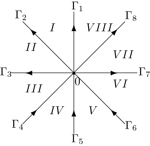

  

  The jump contour $\Sigma _{\mathrm {HG}}$ for $\Phi _{\mathrm {HG}}$. Each of the rays $\Gamma _{1},\ldots ,\Gamma _{8}$ forms an angle with $(0,+\infty )$ which is a multiple of $\frac{\pi }{4}$

• (c) As $z \rightarrow \infty$, $z \notin \Sigma _{\mathrm {HG}}$, we have

  $$\begin{aligned} \Phi _{\mathrm {HG}}(z) = \left( I + \sum _{k=1}^{\infty } \frac{\Phi _{\mathrm {HG},k}}{z^{k}} \right) z^{-\beta \sigma _{3}}e^{-\frac{z}{2}\sigma _{3}}M^{-1}(z), \end{aligned}$$

  (A.6)

  where

  $$\begin{aligned} \Phi _{\mathrm {HG},1} = \Big (\beta ^{2}-\frac{\alpha ^{2}}{4}\Big ) \begin{pmatrix} -1 &{} \tau (\alpha ,\beta ) \\ - \tau (\alpha ,-\beta ) &{} 1 \end{pmatrix}, \qquad \tau (\alpha ,\beta ) = \frac{- \Gamma \left( \frac{\alpha }{2}-\beta \right) }{\Gamma \left( \frac{\alpha }{2}+\beta + 1 \right) },\nonumber \\ \end{aligned}$$

  (A.7)

  and

  $$\begin{aligned} M(z) = \left\{ \begin{array}{l l} \displaystyle e^{\frac{i\pi \alpha }{4} \sigma _{3}}e^{- i\pi \beta \sigma _{3}}, &{} \displaystyle \frac{\pi }{2}< \arg z< \pi , \\ \displaystyle e^{-\frac{i\pi \alpha }{4} \sigma _{3}}e^{-i\pi \beta \sigma _{3}}, &{} \displaystyle \pi< \arg z< \frac{3\pi }{2}, \\ e^{\frac{i\pi \alpha }{4}\sigma _{3}} \begin{pmatrix} 0 &{} 1 \\ -1 &{} 0 \end{pmatrix}, &{} \displaystyle -\frac{\pi }{2}< \arg z< 0, \\ e^{-\frac{i\pi \alpha }{4}\sigma _{3}} \begin{pmatrix} 0 &{} 1 \\ -1 &{} 0 \end{pmatrix},&\displaystyle 0< \arg z < \frac{\pi }{2}. \end{array} \right. \end{aligned}$$

  (A.8)

  In (A.6), $z^{-\beta }$ has a cut along $i{\mathbb {R}}^{-}$, such that $z^{-\beta } \in {\mathbb {R}}$ as $z \in {\mathbb {R}}^{+}$.

  As $z \rightarrow 0$,

  $$\begin{aligned}&\Phi _{\mathrm {HG}}(z) = \left\{ \begin{array}{l l} \begin{pmatrix} {{\mathcal {O}}}(1) &{} {{\mathcal {O}}}(\log z) \\ {{\mathcal {O}}}(1) &{} {{\mathcal {O}}}(\log z) \end{pmatrix}, &{} \text{ if } z \in II \cup III \cup VI \cup VII, \\ \begin{pmatrix} {{\mathcal {O}}}(\log z) &{} {{\mathcal {O}}}(\log z) \\ {{\mathcal {O}}}(\log z) &{} {{\mathcal {O}}}(\log z) \end{pmatrix},&\text{ if } z \in I\cup IV \cup V \cup VIII, \end{array} \right. \nonumber \\&\Phi _{\mathrm {HG}}(z) = \left\{ \begin{array}{l l} \begin{pmatrix} {{\mathcal {O}}}(z^{\frac{\alpha }{2}}) &{} {{\mathcal {O}}}(z^{-\frac{\alpha }{2}}) \\ {{\mathcal {O}}}(z^{\frac{\alpha }{2}}) &{} {{\mathcal {O}}}(z^{-\frac{\alpha }{2}}) \end{pmatrix}, &{} \text{ if } z \in II \cup III \cup VI \cup VII, \\ \begin{pmatrix} {{\mathcal {O}}}(z^{-\frac{\alpha }{2}}) &{} {{\mathcal {O}}}(z^{-\frac{\alpha }{2}}) \\ {{\mathcal {O}}}(z^{-\frac{\alpha }{2}}) &{} {{\mathcal {O}}}(z^{-\frac{\alpha }{2}}) \end{pmatrix},&\text{ if } z \in I\cup IV \cup V \cup VIII, \end{array} \right. \nonumber \\&\Phi _{\mathrm {HG}}(z) = \begin{pmatrix} {{\mathcal {O}}}(z^{\frac{\alpha }{2}}) &{} {{\mathcal {O}}}(z^{\frac{\alpha }{2}}) \\ {{\mathcal {O}}}(z^{\frac{\alpha }{2}}) &{} {{\mathcal {O}}}(z^{\frac{\alpha }{2}}) \end{pmatrix}, \end{aligned}$$

  (A.9)

  where the first, second and third lines read for $\text {Re}\,\alpha = 0$, $\text {Re}\,\alpha > 0$ and $\text {Re}\,\alpha < 0$, respectively.

The unique solution to this RH problem is expressed in terms of hypergeometric functions. Since we will not use the explicit expression of the solution, we will not write it down here. In the case where $\alpha =0$, this RH problem was first solved in [49]. We refer the interested reader to [32, Section 4.2] and [42, Section 2.6] for more details and background on this RH problem for general values of $\alpha$ and $\beta$.

References

Arguin, L.-P., Belius, D., Bourgade, P.: Maximum of the characteristic polynomial of random unitary matrices. Commun. Math. Phys. 349, 703–751 (2017)
Basor, E.: Asymptotic formulas for Toeplitz determinants. Trans. Am. Math. Soc. 239, 33–65 (1978)
Basor, E.: A localization theorem for Toeplitz determinants. Indiana Univ. Math. J. 28, 975–983 (1979)
Berestycki, N., Webb, C., Wong, M.D.: Random hermitian matrices and gaussian multiplicative chaos. Probab. Theory Relat. Fields 172, 103–189 (2018)
Betea, D., Occelli, A.: Discrete and continuous Muttalib–Borodin processes I: the hard edge, arXiv:2010.15529
Bloom, T., Levenberg, N., Totik, V., Wielonsky, F.: Modified logarithmic potential theory and applications. Int. Math. Res. Not. IMRN 2017, 1116–1154 (2017)
Bogatskiy, A., Claeys, T., Its, A.: Hankel determinant and orthogonal polynomials for a Gaussian weight with a discontinuity at the edge. Commun. Math. Phys. 347, 127–162 (2016)
Borodin, A.: Biorthogonal ensembles. Nucl. Phys. B 536, 704–732 (1999)
Borot, G., Guionnet, A., Kozlowski, K.K.: Large-\(N\) asymptotic expansion for mean field models with Coulomb gas interaction. Int. Math. Res. Not. IMRN 2015, 10451–10524 (2015)
Böttcher, A., Silbermann, B.: Toeplitz operators and determinants generated by symbols with one Fisher–Hartwig singularity. Math. Nachr. 127, 95–123 (1986)
Bourgade, P., Mody, K., Pain, M.: Optimal local law and central limit theorem for \(\beta \)-ensembles. arXiv:2103.06841
Breuer, J., Duits, M.: Central limit theorems for biorthogonal ensembles and asymptotics of recurrence coefficients. J. Am. Math. Soc. 30, 27–66 (2017)
Charlier, C.: Asymptotics of Hankel determinants with a one-cut regular potential and Fisher–Hartwig singularities. Int. Math. Res. Not. IMRN 2019, 7515–7576 (2019)
Charlier, C.: Exponential moments and piecewise thinning for the Bessel point process. Int. Math. Res. Not. IMRN, rnaa054
Charlier, C.: Large gap asymptotics for the generating function of the sine point process. Proc. Lond. Math. Soc., plms.12393
Charlier, C.: Upper bounds for the maximum deviation of the Pearcey process. Rand. Mat. Theory Appl. https://doi.org/10.1142/S2010326321500398, arXiv:2009.13225
Charlier, C., Claeys, T.: Large gap asymptotics for Airy kernel determinants with discontinuities. Commun. Math. Phys. 375, 1299–1339 (2020)
Charlier, C., Claeys, T.: Global rigidity and exponential moments for soft and hard edge point processes. Prob. Math. Phys. arXiv:2002.03833
Charlier, C., Deaño, A.: Asymptotics for Hankel determinants associated to a Hermite weight with a varying discontinuity. SIGMA Symm. Integrabil. Geom. Methods Appl. 14, 43 (2018)
Charlier, C., Gharakhloo, R.: Asymptotics of Hankel determinants with a Laguerre-type or Jacobi-type potential and Fisher–Hartwig singularities. Adv. Math. 383, j.aim.2021.107672
Charlier, C., Lenells, J., Mauersberger, J.: Higher order large gap asymptotics at the hard edge for Muttalib–Borodin ensembles. Commun. Math. Phys. arXiv:1906.12130
Chhaibi, R., Madaule, T., Najnudel, J.: On the maximum of the C\(\beta \)E field. Duke Math. J. 167, 2243–2345 (2018)
Cheliotis, D.: Triangular random matrices and biorthogonal ensembles. Statist. Probab. Lett. 134, 36–44 (2018)
Claeys, T., Fahs, B.: Random matrices with merging singularities and the Painlevé V equation. SIGMA Symm. Integrabil. Geom. Methods Appl. 12, 44 (2016)
Claeys, T., Fahs, B., Lambert, G., Webb, C.: How much can the eigenvalues of a random Hermitian matrix fluctuate? Duke Math J. arxiv:1906.01561
Claeys, T., Girotti, M., Stivigny, D.: Large gap asymptotics at the hard edge for product random matrices and Muttalib–Borodin ensembles. Int. Math. Res. Not. IMRN 2019, 2800–2847 (2019)
Claeys, T., Glesner, G., Minakov, A., Yang, M.: Asymptotics for averages over classical orthogonal ensembles. Int. Math. Res. Not. arxiv:2008.07785
Claeys, T., Romano, S.: Biorthogonal ensembles with two-particle interactions. Nonlinearity 27(10), 2419–2444 (2014)
Claeys, T., Wang, D.: Random matrices with equispaced external source. Commun. Math. Phys. 328(3), 1023–1077 (2014)
Dai, D., Xu, S.-X., Zhang, L.: On the deformed Pearcey determinant. arXiv:2007.12691
Deift, P.: Orthogonal polynomials and random matrices: a Riemann-Hilbert approach. Am. Math. Soc. 3 (2000)
Deift, P., Its, A., Krasovky, I.: Asymptotics of Toeplitz, Hankel, and Toeplitz+Hankel determinants with Fisher–Hartwig singularities. Ann. Math. 174, 1243–1299 (2011)
Deift, P., Its, A., Krasovsky, I.: On the asymptotics of a Toeplitz determinant with singularities. MSRI Publications65 (2014), Cambridge University Press
Deift, P., Zhou, X.: A steepest descent method for oscillatory Riemann–Hilbert problems. Asymptotics for the MKdV equation. Ann. Math. 137, 295–368 (1993)
Ehrhardt, T.: A status report on the asymptotic behavior of Toeplitz determinants with Fisher–Hartwig singularities. Oper. Theory Adv. Appl. 124, 217–241 (2001)
Eichelsbacher, P., Sommerauer, J., Stolz, M.: Large deviations for disordered bosons and multiple orthogonal polynomial ensembles. J. Math. Phys. 52, 16 (2011)
Erdös, L., Yau, H.-T., Yin, J.: Rigidity of eigenvalues of generalized Wigner matrices. Adv. Math. 229, 1435–1515 (2012)
Fisher, M.E., Hartwig, R.E.: Toeplitz determinants: some applications, theorems, and conjectures. Adv. Chem. Phys. 15, 333–353 (1968)
Forrester, P.J., Ipsen, J.R.: Selberg integral theory and Muttalib–Borodin ensembles. Adv. Appl. Math. 95, 152–176 (2018)
Forrester, P.J., Liu, D.-Z.: Raney distributions and random matrix theory. J. Stat. Phys. 158, 1051–1082 (2015)
Forrester, P.J., Wang, D.: Muttalib–Borodin ensembles in random matrix theory-realisations and correlation functions. Electron. J. Probab. 22, 43 (2017)
Foulquié Moreno, A., Martinez-Finkelshtein, A., Sousa, V.L.: On a conjecture of A Magnus concerning the asymptotic behavior of the recurrence coefficients of the generalized Jacobi polynomials. J. Approx. Theory 162, 807–831 (2010)
Gakhov, F.D.: Boundary value problems, Dover Publications Inc., New York, (1990). Translated from the Russian, Reprint of the 1966 translation
Garoni, T.M.: On the asymptotics of some large Hankel determinants generated by Fisher–Hartwig symbols defined on the real line. J. Math. Phys. 46, 19 (2005)
Gautié, T., Le Doussal, P., Majumdar, S.N., Schehr, G.: Non-crossing Brownian paths and Dyson Brownian motion under a moving boundary. J. Stat. Phys. 177, 752–805 (2019)
Grela, J., Majumdar, S.N., Schehr, G.: Non-intersecting Brownian bridges in the flat-to-flat geometry. arXiv:2103.02545
Gustavsson, J.: Gaussian fluctuations of eigenvalues in the GUE. Ann. Inst. H. Poincare Probab. Statist. 41, 151–178 (2005)
Holcomb, D., Paquette, E.: The maximum deviation of the Sine-\(\beta \) counting process. Electron. Commun. Probab. 23, 13 (2018). (paper no. 58)
Its, A., Krasovsky, I.: Hankel determinant and orthogonal polynomials for the Gaussian weight with a jump. Contemp. Math. 458, 215–248 (2008)
Krasovsky, I.: Correlations of the characteristic polynomials in the Gaussian unitary ensemble or a singular Hankel determinant. Duke Math. J. 139, 581–619 (2007)
Kuijlaars, A.B.J.: A vector equilibrium problem for Muttalib–Borodin biorthogonal ensembles. SIGMA Symm. Integrabil. Geom. Methods Appl. 12, 15 (2016)
Kuijlaars, A.B.J., Molag, L.D.: The local universality of Muttalib–Borodin biorthogonal ensembles with parameter \(\theta = \frac{1}{2}\). Nonlinearity 32, 3023–3081 (2019)
Kuijlaars, A.B.J., McLaughlin, K.T.-R., Van Assche, W., Vanlessen, M.: The Riemann–Hilbert approach to strong asymptotics for orthogonal polynomials on \([-1,1]\). Adv. Math. 188, 337–398 (2004)
Kuijlaars, A.B.J., Stivigny, D.: Singular values of products of random matrices and polynomial ensembles. Rand. Mat. Theory Appl. 3, 22 (2014)
Lambert, G.: Limit theorems for biorthogonal ensembles and related combinatorial identities. Adv. Math. 329, 590–648 (2018)
Lambert, G.: Mesoscopic central limit theorem for the circular beta-ensembles and applications. Electron. J. Probab. 26, 33 (2021)
Molag, L.D.: The local universality of Muttalib–Borodin ensembles when the parameter \(\theta \) is the reciprocal of an integer. arXiv:2003.11299
Muttalib, K.A.: Random matrix models with additional interactions. J. Phys. A 28, L159–L164 (1995)
Paquette, E., Zeitouni, O.: The maximum of the CUE field. Int. Math. Res. Not. 2018(16), 5028–5119 (2018)
Saff, E.B., Totik, V.: Logarithmic Potentials with External Fields. Springer, New York (1997)
Soshnikov, A.: Gaussian fluctuation for the number of particles in Airy, Bessel, sine, and other determinantal random point fields. J. Stat. Phys. 100, 491–522 (2000)
Wang, D., Zhang, L.: A vector Riemann–Hilbert approach to the Muttalib–Borodin ensembles. arXiv:2103.10327
Widom, H.: Toeplitz determinants with singular generating functions. Am. J. Math. 95, 333–383 (1973)
Wu, X.-B., Xu, S.-X., Zhao, Y.-Q.: Gaussian unitary ensemble with boundary spectrum singularity and \(\sigma \)-form of the Painlevé II equation. Stud. Appl. Math. 140, 221–251 (2018)
Zhang, L.: Local universality in biorthogonal Laguerre ensembles. J. Stat. Phys. 161, 688–711 (2015)
Zhang, L.: On Wrights generalized Bessel kernel. Phys. D 340, 27–39 (2017)
Acknowledgements
The author is grateful to Tom Claeys for useful remarks. This work is supported by the European Research Council, Grant Agreement No. 682537.
Author information
Authors and Affiliations
Additional information
Publisher's Note
Springer Nature remains neutral with regard to jurisdictional claims in published maps and institutional affiliations.