Compact Proof Witnesses

Abstract

Proof witnesses are proof artifacts showing correctness of programs wrt. safety properties. The recent past has seen a rising interest in witnesses as (a) proofs in a proof-carrying-code context, (b) certificates for the correct functioning of verification tools, or simply (c) exchange formats for (partial) verification results. As witnesses in all theses scenarios need to be stored and processed, witnesses are required to be as small as possible. However, software verification tools – the prime suppliers of witnesses – do not necessarily construct small witnesses.

In this paper, we present a formal account of proof witnesses. We introduce the concept of weakenings, reducing the complexity of proof witnesses while preserving the ability of witnessing safety. We develop a weakening technique for a specific class of program analyses, and prove it to be sound. Finally, we experimentally demonstrate our weakening technique to indeed achieve a size reduction of proof witnesses.

1 Introduction

In the past years, automatic verification of programs with respect to safety properties has reached a level of maturity that makes it applicable to industrial-size programs. The annual software verification competition SV-COMP [4] demonstrates the advances of program verification, in particular its scalability. Software verification tools prove program correctness, most often for safety properties written into the program in the form of assertions. When the verification tool terminates, the result is typically a yes/no answer optionally accompanied by a counterexample. While this is the obvious result a verification tool should deliver, it became clear in recent years that all the information computed about a program during verification is too valuable to just be discarded at the end. Such information should better be stored in some form of proof.

Proofs are interesting for several reasons: (A) Proofs can be used in a proof-carrying code (PCC) context [25] where a program is accompanied by its proof of safety. Verifying this proof allows to more easily recheck the safety of the program, e.g., when its provider is untrusted. (B) A proof can testify that the verification tool worked correctly, and checking the proof gives confidence in its soundness [5]. (C) Verification tools are sometimes unable to complete proving (e.g., due to timeouts). A proof can then summarize the work done until the tool stopped (see e.g. [6]) so that other tools can continue the work. All these scenarios use proofs as witnesses of the (partial) correctness of the program.

For these purposes, witnesses need to be small. If the witness is very large, the gain of having a witness and thus not needing to start proving from scratch is lost by the time and memory required to read and process the witness. Our interest is thus in compact proof witnesses. However, the proof artifacts that software verification tools produce are often even larger than the program itself.

Large proofs are a well-known problem in PCC approaches (e.g. [1, 2, 22, 24, 26, 29]). To deal with the problem, Necula and Lee [24] (who employ other types of proofs than automatic verification tools produce) use succinct representations of proofs. A different practice is to store only parts of a proof and recompute the remaining parts during proof validation like done by Rose [28] or Jakobs [22]. An alternative approach employs techniques like lazy abstraction [9, 20] to directly construct small proofs. Further techniques as presented by Besson et al. [2] and Seo et al. [29] try to remove irrelevant information from proofs that are fixpoints. The latter two approaches have, however, only looked at proofs produced by path-insensitive program analyses.

In this paper, we first of all present a formal account of proof witnesses. We do so for verification tools generating for the safety analysis some form of abstract state space of the program, either by means of a path insensitive or a path sensitive analysis. We call this abstract reachability graph in the sequel, following the terminology for the software verification tool CPAchecker [8]. We formally state under what circumstances proof witnesses can actually soundly testify program safety. Based on this, we study weakenings of proof witnesses, presenting more compact forms of proofs while preserving being a proof witness. Next, we show how to compute weakenings for a specific category of program analyses. Finally, we experimentally show our weakening technique to be able to achieve size reduction of proof witnesses. To this end, we evaluated our weakening technique on 395 verification tasks taken from the SV-COMP [3] using explicit-state software model checking as analysis method for verification. Next to proof size reduction, we also evaluate the combination of our approach with lazy refinement [9] plus examine its performance in a PCC setting [22].

2 Background

Witnesses are used to certify safety of programs. In this section, we start with explaining programs and their semantics. For this presentation, we assume to have programs with assignments and assume statements (representing if and while constructs) and with integer variables only¹. We distinguish between boolean expressions used in assume statements, and abbreviate assume bexpr simply by bexpr, and arithmetic expressions aexpr used in assignments. The set $Ops$ contains all these statements, and the set $Var$ is the set of variables occuring in a program. Following Configurable Software Verification [7] – the technique the tool CPAchecker, in which we integrated our approach, is based on –, we model a program by a control-flow automaton (CFA) $P=(L,E_{ CFA }, \ell _0, L_{\mathrm {err}})$. The set $L$ represents program locations, $\ell _0$ is the initial program location, and $E_{ CFA }\subseteq L\times Ops\times L$ models the control-flow edges. The set $L_\mathrm {err}\subseteq L$ of error locations defines which locations are unsafe to reach. In the program, these safety properties are written as assert statements. Note that all safety properties can be encoded this way [23], and that we assume that all properties of interest are encoded at once.

Fig. 1.

Program $\mathsf {isZero}$ (i input variable) and its control-flow automaton

Figure 1 gives a small (completely artificial) program called $\mathsf {isZero}$ (which we use later for explanation) and its control-flow automaton. Here, location $\ell _{e}$ is the only error location. The program is called $\mathsf {isZero}$ since it tests whether the input $\texttt {i}$ is zero (which is recorded as value 1 in r). The assertion checks whether the number of assignments to r or checks on r is 3 when r is 1. This number is accumulated in the variable c.

The semantics of a program $P=(L,E_{ CFA },\ell _0,L_\mathrm {err})$ is defined by a labeled transition system $(L\times C,E_{ CFA },\rightarrow )$ made up of a set of concrete states $C$ plus locations L, the labels $E_{ CFA }$ (the control-flow edges of the program) and a transition relation $\mathop {\rightarrow } \subseteq (L\times C) \times E_{ CFA }\times (L\times C)$. We write $(\ell ,c)\mathop {\rightarrow }\limits ^{e}(\ell ',c')$ for $((\ell ,c),e,(\ell ',c'))\in \mathbin {\rightarrow }$. A concrete state in C is a mapping $c: Var \rightarrow \mathbb {Z}$. A transition $(\ell ,c)\xrightarrow {(\ell ,op,\ell ')}(\ell ',c')$ is contained in the transition relation $\rightarrow$ if either $op\equiv bexpr$, $c(bexpr)=true$ ² and $\forall v\in Var : c(v)=c'(v)$, or $op\equiv x:=aexpr$, $c'(x)=c(aexpr)$, and $\forall v\in Var \setminus \{x\}: c(v)=c'(v)$. We call $(\ell _0,c_0)\mathop {\rightarrow }\limits ^{e_1}(\ell _1,c_1)\dots \mathop {\rightarrow }\limits ^{e_n}(\ell _n,c_n)$ a path of P if $(\ell _i,c_i)\mathop {\rightarrow }\limits ^{e_i}(\ell _{i+1},c_{i+1})$, $1\le i< n$, is a transition in $T_P$. The set of all paths, i.e. (partial) program executions, of program $P$ is denoted by $paths_P$. Finally, a program is safe if no program execution reaches an error location, i.e., $\forall (\ell _0,c_0)\mathop {\rightarrow }\limits ^{e_1}(\ell _1,c_1)\dots \mathop {\rightarrow }\limits ^{e_n}(\ell _n,c_n)\in paths_P: \ell _n \notin L_\mathrm {err}$.

We build our technique for witness compaction on top of the configurable program analysis (CPA) framework of Beyer et al. [7] which allows to specify customized, abstract interpretation based program analyses. The advantage of using CPAs is that our results are not just valid for one analysis, but for a whole range of various analyses (namely those specifiable as CPAs). A CPA for a program $P$ is a four-tuple $\mathbb {A} = (D,\rightsquigarrow ,\mathsf {merge}, \mathsf {stop})$ containing

• 1. an abstract domain $D=(C, \mathcal {A},[\![\cdot ]\!])$ consisting of a set $C$ of concrete states, a complete lattice $\mathcal {A} = (A, \top , \bot , \sqsubseteq , \sqcup , \sqcap )$ on a set of abstract states $A$ and a concretization function $[\![\cdot ]\!]: A\rightarrow 2^{C}$, with

  

• 2. a transfer function $\mathop {\rightsquigarrow }\subseteq A\times E_{ CFA } \rightarrow A$ defining the abstract semantics: $\forall a \in A, e\in E_{ CFA }$ s.t. $\mathop {\rightsquigarrow }(a, e) = a'$

  $$\begin{aligned}\begin{gathered} \{c'\mid c\in [\![a]\!]\wedge \exists \ell , \ell ': (\ell ,c)\mathop {\rightarrow }\limits ^{e}(\ell ',c')\}\subseteq [\![a']\!], \end{gathered}\end{aligned}$$

• 3. a merge operator $\mathsf {merge}$ and a termination check operator $\mathsf {stop}$ steering the construction of the abstract state space, and satisfying (a) $\forall a,a' \in A: a'\sqsubseteq \mathsf {merge}(a,a')$ and (b) $\forall a\in A, S \subseteq A: \mathsf {stop}(a, S)\implies \exists a'\in S: a\sqsubseteq a'$. Both of these operators will play no role in the following, and are thus not further discussed here.

Based on a given analysis $\mathbb {A}$, an abstract state space of a given program is then constructed in the form of an abstract reachability graph (ARG). To this end, the initial abstract state $a_0 \in \mathcal{A}$ is fixed to be $\top$, and the root of the ARG becomes $(\ell _0,a_0)$. The ARG is then further constructed by examining the edges of the CFA and computing successors of nodes under the transfer function of the analysis $\mathbb {A}$. The stop operator fixes when to end such an exploration. An ARG for a program $P = (L,E_{ CFA },\ell _0,L_\mathrm {err})$ is thus a graph $G=(N,E_ ARG ,root)$ with nodes being pairs of locations and abstract values, i.e., $N \subseteq L \times A$ and edges $E_ ARG \subseteq N \times E_{ CFA } \times N$. We say that two nodes $n_1 = (\ell _1,a_1)$ and $n_2 = (\ell _2,a_2)$ are location equivalent, $n_1 =_{loc} n_2$, if $\ell _1 = \ell _2$. We lift the ordering on elements in A to elements in $L \times A$ by saying that $(\ell _1,a_1) \sqsubseteq (\ell _2,a_2)$ if $\ell _1 = \ell _2$ and $a_1 \sqsubseteq a_2$. We write $n \mathop {\rightarrow }\limits ^{e} n'$, $e \in E_{ CFA }$, if $(n,e,n') \in E_ ARG$, and $n \mathop {\rightsquigarrow }\limits ^{e} n'$ if $n=(\ell ,a)$, $n'=(\ell ',a')$, $e=(\ell ,op,\ell ') \in E_{ CFA }$ and $a \mathop {\rightsquigarrow }\limits ^{e} a'$.

3 Proof Witnesses and Weakenings

Abstract reachability graphs represent overapproximations of the state space of the program. They are used by verification tools for inspecting safety of the program: if no error location is reachable in the ARG, it is also unreachable in the program, and the tool can then testify safety. Thus, ARGs are excellent candidates for proof witnesses. However, our definition of an ARG only fixes the syntactical appearance and allows ARGs that are not necessarily proper proof witnesses (and real overapproximations), e.g., our definition allows that an ARG could simply have ignored the exploration of certain edges in the CFA.

Definition 1

An ARG G constructed by an analysis $\mathbb {A}$ is a proof witness for program P if the following properties hold:

• Rootedness. The root node root $(\ell _0,\top )$,

• Soundness. All successor nodes are covered:

  $$\begin{aligned} \forall n \in N: n \mathop {\rightsquigarrow }\limits ^{e} n'\ implies\ \exists n'': n \mathop {\rightarrow }\limits ^{e} n'' \wedge n' \sqsubseteq n'', \end{aligned}$$

• Safety. No error nodes are present: $\forall (\ell ,\cdot ) \in N: \ell \notin L_{err}$.

(Sound) verification tools construct ARGs which are indeed proof witnesses (unless the program is not safe). When such an ARG is used as a proof witness, safety of the program can then be checked by validating the above three properties for the ARG. Such checks are often less costly than building a new ARG from scratch. This makes proof witnesses excellent candidates for proofs in a proof-carrying code setting.

Proposition 1

If an ARG G is a proof witness for program P, then P is safe.

However, ARGs are often unnecessarily complex witnesses. They often store information about program variables that is either too detailed or even not needed at all. Our interest is thus in finding smaller witnesses. In terms of the analysis, too much detail means that the information stored for program locations is unnecessarily low in the lattice ordering $\sqsubseteq$. We build our compaction technique on the following assumption about the size of witnesses.

Assumption. The weaker (i.e., the higher in the lattice ordering) the abstract values stored for program locations, the more compact the witness.

As an example justifying this assumption take the weakest element $\top$: as it represents the whole set of concrete states, it brings us no specific information at all and can thus also be elided from a witness. This assumption is also taken in the work of Besson et al. [2]. We base the following approach on the assumption – which our experiments also confirm – and define weakenings for proof witnesses.

Definition 2

A function $w: L \times A \rightarrow L \times A$ is a weakening function for a domain $D = (C,\mathcal{A},[\![\cdot ]\!])$ and program $P= (L,E_{ CFA },\ell _0,L_\mathrm {err})$ if it satisfies the following two properties:

• $(\ell ,a) \sqsubseteq w(\ell ,a)$ (weakening),

• $w(\ell ,a) =_{loc} (\ell ,a)$ (location preserving).

A weakening function for D and P is consistent with the transfer function if the following holds:

• for all $e\in E_{ CFA }$, $n \in L \times A$: $w(n) \mathop {\rightsquigarrow }\limits ^{e}$ implies $n\mathop {\rightsquigarrow }\limits ^{e}$,

• for all $n_1 \in L \times A$: if $w(n_1) = n_1'$ and $n_1' \mathop {\rightsquigarrow }\limits ^{e} n_2'$, then for $n_2 \text{ s.t. } n_1 \mathop {\rightsquigarrow }\limits ^{e} n_2$: $n_2' \sqsubseteq w(n_2)$.

While formally being similar to widenings [13] used in program analysis during fixpoint computation, weakenings serve a different purpose. And indeed, widening functions are too limited for being weakenings as they do not take the program under consideration into account.

Weakening functions are applied to ARGs just by applying them to all nodes and edges: for an ARG G, $w(G)=(w(N),w(E),w(root))$, where $w(E) = \{ (w(n_1),e,w(n_2)) \mid (n_1,e,n_2) \in E_ ARG \}$. Note that $w(root) = root$ since the root already uses the top element in the lattice.

Theorem 1

If an ARG G is a proof witness for program P and w is a weakening function for D and P consistent with the transfer function, then w(G) is a proof witness for program P as well.

Proof

We use the following notation: $G=(N,E,root)$ is the ARG, $w(G) = (w(N),$ $w(E),w(root)) = (N',E',root')$ its weakening. We need to show the three properties of proof witnesses to be valid in w(G).

• Soundness. The most interesting property is soundness. We need to show that $\forall n_1' \mathop {\rightsquigarrow }\limits ^{e} n'_2, n_1' \in N'$, there is an $n_3' \in N': n_1' \mathop {\rightarrow }\limits ^{e} n_3' \wedge n_2' \sqsubseteq n_3'$.

  Let $n_1 \in N$ be the node with $w(n_1) = n_1'$.

  $$\begin{aligned}\begin{gathered} w(n_1) \mathop {\rightsquigarrow }\limits ^{e} n_2' \\ \Rightarrow \{ \text{ w } \text{ consistent } \text{ with } \text{ transfer } \text{ function } \} \\ \exists \hat{n}: n_1 \mathop {\rightsquigarrow }\limits ^{e} \hat{n} \\ \Rightarrow \{ \text{ soundness } \text{ of } \text{ G } \} \\ \exists n_2 \in N: n_1 \mathop {\rightarrow }\limits ^{e} n_2 \wedge \hat{n} \sqsubseteq n_2 \\ \Rightarrow \{ \text{ construction } \text{ of } G' \} \\ w(n_1) \mathop {\rightarrow }\limits ^{e} w(n_2) \text{ in } G' \\ \Rightarrow \{ \text{ w } \text{ consistent } \text{ with } \text{ transfer } \text{ function } \} \\ n_2' \sqsubseteq w(n_2) \end{gathered}\end{aligned}$$

  Thus, choose $n_3':= w(n_2)$.

• Rootedness, Safety. Both follow by w being a weakening function, and w(G) being constructed by applying w on all nodes of the ARG.

4 Variable-Separate Analyses

The last section introduced proof witnesses, and showed that we get a smaller, yet proper proof witness when using a weakening consistent with the transfer function. Next, we show how to define such weakening functions for a specific sort of program analyses $\mathbb {A}$. In the following, we study analyses that use mappings of program variables to abstract values as its abstract domain D. We call such analyses variable-separate because they separately assign values to variables. Examples of variable-separating analyses are constant propagation and explicit-state model checking (both assigning concrete values to variables), interval analysis (assigning intervals to variables), sign analysis (assigning signs to variables), or arithmetical congruence (assigning a congruence class $\bar{c}_m$ to variables, i.e., variable value is congruent to c modulo m).

Definition 3

A variable-separate analysis consists of a base domain $(B,\top _B,\bot _B$, $\sqsubseteq _B,\sqcup _B,\sqcap _B)$ that is a complete lattice equipped with an evaluation function $eval_B$ on variable-free expressions such that

• $eval_B(bexpr) \in 2^{\{ true,false \}} \setminus \emptyset$ and

• $eval_B(aexpr) \in B$,

for $vars(aexpr) = vars(bexpr) = \emptyset$.

B is lifted to the variable-separate analysis with domain $A = B^{ Var }$ where

• $a_1 \sqsubseteq _A a_2$ is obtained by pointwise lifting of $\sqsubseteq _B$:

  $\forall v\in Var : a_1(v) \sqsubseteq _B a_2(v)$,

• expression evaluation is obtained by replacing variables with their values: $a(expr) = eval_B(expr[v \mapsto a(v) \mid v \in vars(expr) ] )$,

• $a_1 \mathop {\rightsquigarrow }\limits ^{bexpr} a_2$ if $true \in a_1(bexpr)$ and

  

• $a_1 \mathop {\rightsquigarrow }\limits ^{x:=aexpr} a_2$ if $a_2(y) = a_1(y)$ for $y \ne x$ and $a_2(x) = a_1(aexpr)$.

Note that the execution of an assume statement (bexpr) further constrains the successor state to those satisfying bexpr. The analysis uses the meet operator $\sqcap$ for this. As an example analysis in our experiments, we use explicit-state model checking [15]. It tracks precise values of variables, however, if combined with lazy refinement [9] it does not track all but just some variables, and therefore does not plainly build the complete state space of a program.

Example 1

Explicit-state model checking uses the flat lattice $B=\mathbb {Z} \cup \{ \top , \bot \}$ with $\bot \sqsubseteq b$ and $b \sqsubseteq \top$ for all $b\in B$, all other elements are incomparable. The operators $\sqcup$ and $\sqcap$ are the least upper bound and greatest lower bounds operators, respectively. Assigning $\top$ to a variable amounts to not tracking the value of that variable or the analysis failed to determine a precise, concrete value. The evaluation function computes the usual arithmetic semantics (denoted $[\![expr ]\!]$), except on $\top$ elements (which can appear in expressions when variables are instantiated according to an abstract value).

$$ eval_B(bexpr) \ni \left\{ \begin{array}{ll} true &{} \text{ if } \exists z_i \in \mathbb {Z}: [\![bexpr[\top _i \mapsto z_i] ]\!] = true \\ false &{} \text{ if } \exists z_i \in \mathbb {Z}: [\![bexpr[\top _i \mapsto z_i] ]\!] = false \end{array} \right. $$

Here, we write $[\![expr[\top _i \mapsto z_i] ]\!]$ for replacing all $\top$ occurrences in expr by (possibly different) elements from $\mathbb {Z}$.

$$\begin{aligned} eval_B(aexpr) = {\left\{ \begin{array}{ll} [\![aexpr ]\!] &{} \text {if no } \top \text { in } aexpr \\ \top &{} \text {else} \end{array}\right. } \end{aligned}$$

Figure 2 shows the ARG computed for program $\mathsf {isZero}$ when using explicit-state model checking without lazy refinement. We directly elide variables which are mapped to $\top$ as these will not be stored in a proof witness.

Fig. 2.

ARG of program $\mathsf {isZero}$ using explicit-state model checking

Fig. 3.

Weakened witness of program $\mathsf {isZero}$

For variable-separate analyses, we obtain weakenings by computing the set of variables relevant at an ARG node. This is similar to the computation of live variables [27], where, however, the variables to be tracked are tailored towards not introducing new paths in the weakening that were not present in the ARG. The computation of relevant variables has similiarities with program slicing [30] as we compute backward dependencies of variables. For $(\ell ,a) \in N$, we define

• ,

• $-\ trans_{(\ell ,op,\ell ')}(V_{\ell '}) := \left\{ \begin{array}{l} (V_{\ell '} \setminus \{x\}) \cup vars(aexpr) \\ \quad \text{ if } op\equiv x:=aexpr \wedge x \in V_{\ell '} \\ V_{\ell '} \cup vars(bexpr) \\ \quad \text{ if } op\equiv bexpr \wedge vars(bexpr) \cap V_{\ell '} \ne \emptyset \\ V_{\ell '} \text{ else } \end{array} \right.$

The definition of init aims at keeping those variables for which the ARG has already determined that a syntactically possible outgoing edge is semantically impossible; the definition of trans propagates these sets backwards via dependencies. Together, this gives rise to a family of equations $(rel_{(\ell ,a)})_{(\ell ,a) \in N}$ for the nodes in the ARG:

$$\begin{aligned} rel_{(\ell ,a)} = \Big ( init(\ell ,a) \cup \bigcup _{\big ((\ell ,a),e,(\ell ',a')\big ) \in E_ ARG } trans_e(rel_{(\ell ',a')})\Big )\setminus \{ v\in Var \mid a(v) = \top \} \end{aligned}$$

Note that we remove all variables from this set that are assigned $\top$ in a, since no knowledge from previous nodes is required to compute this information. We use $(Rel_{(\ell ,a)})_{(\ell ,a) \in N}$ to stand for the smallest solution to this equation system that can be computed by a fixpoint computation starting with the emptyset of relevant variables for all nodes³.

Definition 4

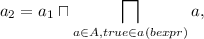
Let $(Rel_{(\ell ,a)})_{(\ell ,a) \in N}$ be the family of relevant variables. We define the weakening wrt. Rel for nodes $(\ell ,a) \in N$ as

$$ \mathsf {weaken}_{Rel}(\ell ,a) := (\ell ,a') \text{ with } a'(v) = \left\{ \begin{array}{ll} \top _B &{} \text{ if } v \notin Rel_{(\ell ,a)} \\ a(v) &{} \text{ else } \end{array} \right. $$

For all $(\ell ,a) \notin N$, we set $\mathsf {weaken}(\ell ,a) := (\ell ,a)$.

Figure 3 shows the weakened ARG for program $\mathsf {isZero}$. We see that in several abstract states fewer variables have to be tracked. Due to init, the weakened ARG tracks variables $r$ and $c$ at locations $\ell _6$ and $\ell _7$. Furthermore, it tracks those values required to determine the values of these variables at those locations.

The key result of this section states that this construction indeed defines a weakening function consistent with the transfer function.

Theorem 2

Let G be an ARG of program P constructed by a variable-separate analysis, $(Rel_n)_{n\in N}$ the family of relevant variables. Then $\mathsf {weaken}_{Rel}$ is a weakening function for G consistent with $\mathop {\rightsquigarrow }\limits ^{}$.

This theorem follows from the following observations and lemmas: (a) $(\ell ,a) \sqsubseteq _A \mathsf {weaken}_{Rel}(\ell ,a)$ follows from $\top _B$ being the top element in the lattice B, and (b) $\mathsf {weaken}_{Rel}(\ell ,a) =_{loc} (\ell ,a)$ by definition of $\mathsf {weaken}$.

Lemma 1

Let $n \in N$ be an ARG node, $e \in E_{ CFA }$ an edge. Then $\mathsf {weaken}_{Rel}(n) \mathop {\rightsquigarrow }\limits ^{e}$ implies $n \mathop {\rightsquigarrow }\limits ^{e}$.

Proof

Let $e=(\ell ,op,\ell ')$, $op = bexpr$, $n=(\ell ,a)$ (otherwise the CFA would already forbid an edge), $\mathsf {weaken}(\ell ,a) = (\ell ,a')$. Proof by contraposition.

Lemma 2

Let $n_1 \in N$ be a node of the ARG. If $\mathsf {weaken}(n_1) = n_1'$ and $n_1 \mathop {\rightsquigarrow }\limits ^{e} n_2$, then $\forall n_2'$ such that $n_1' \mathop {\rightsquigarrow }\limits ^{e} n_2'$ we get $n_2' \sqsubseteq \mathsf {weaken}(n_2)$.

Proof

Let $n_1=(\ell _1,a_1), n_2 = (\ell _2,a_2), n_1'=(\ell _1,a_1'), n_2' = (\ell _2,a_2')$, $e=(\ell _1,op,\ell _2)$. Let furthermore $V_2 = Rel_{(\ell _2,a_2)}$ and $V_1 = Rel_{(\ell _1,a_1)}$.

• Case 1. $op \equiv x:=aexpr$.

• $x \in V_2$: Then by definition of Rel, $vars(aexpr) \setminus \{ v \in Var \mid a_1(v) = \top \} \subseteq V_1$. We have to show $n_2' \sqsubseteq \mathsf {weaken}(n_2)$. We first look at x.

  $$\begin{aligned}\begin{gathered} a_2'(x) \\ = \{ \text{ def. } \mathop {\rightsquigarrow }\limits ^{} \} \\ a_1'(aexpr) \\ = \{ \text{ def. } \text{ weaken, } \quad vars(aexpr) \setminus \{ v \in Var \mid a_1(v) = \top \} \subseteq V_1 \ \} \\ a_1(aexpr) \\ = \{ \text{ def. } \mathop {\rightsquigarrow }\limits ^{} \} \\ a_2(x) \\ \sqsubseteq \{ \text{ def. } \text{ weaken } \} \\ \mathsf {weaken}(a_2)(x) \end{gathered}\end{aligned}$$

  Next $y \ne x$, $y \in V_1$.

  $$\begin{aligned}\begin{gathered} a_2'(y) \\ = \{ \text{ definition } \mathop {\rightsquigarrow }\limits ^{}\text{, } y\ne x \} \\ a_1'(y) \\ = \{ \text{ def. } \text{ weaken } \} \\ a_1(y) \\ = \{ \text{ def. } \mathop {\rightsquigarrow }\limits ^{} \} \\ a_2(y) \\ \sqsubseteq \{ \text{ def. } \text{ weaken } \} \\ \mathsf {weaken}(a_2)(y) \end{gathered}\end{aligned}$$

  Next $y\ne x, y \notin V_1$. Note that by definition of Rel, $y \notin V_2$, hence $a_1'(y) = \top _B = \mathsf {weaken}(a_2)(y)$.

• $x \notin V_2$: We have $a_2'(x) \sqsubseteq \mathsf {weaken}(a_2)(x)$ since $\mathsf {weaken}(a_2)(x) = \top _B$ by definition of weaken. The case for $y\ne x$ is the same as for $x\in V_2$.

• Case 2. $op \equiv bexpr$. Similar to case 1, using the fact that if $a_1(y) = a_1'(y)$ then

  

5 Experiments

The last section has introduced a technique for computation of weakenings. Next, we experimentally evaluate this weakening technique for the explicit-state model checking analysis. In our experiments, we wanted to study three questions:

• Q1. Does weakening reduce the size of proof witnesses?

• Q2. Does explicit-state model checking with lazy refinement [9] benefit from weakening?

• Q3. Do PCC approaches benefit from ARG weakenings?

To explain question 2: Lazy refinement already aims at “lazily” including new variables to be tracked, i.e., as few as possible. The interesting question is thus whether our weakenings can further reduce the variables. For question 3, we employed an existing ARG-based PCC technique [22]. To answer these questions, we integrated our ARG weakening within the tool CPAchecker [8] and evaluated it on category Control Flow and Integer Variables of the SV-COMP [3]. We excluded all programs that were not correct w.r.t. the specified property, or for which the verification timed out after 15 min, resulting in 395 programs (verification tasks) in total. For explicit-state model checking with and without lazy refinement we used the respective standard value analyses provided by CPAchecker. Both analyses generate ARGs.

We run our experiments within BenchExec [10] on an Intel$^{\textregistered }$ Xeon E3-1230 v5 @ 3.40 GHz and OpenJDK 64-Bit Server VM 1.8.0_121 restricting each task to 5 of 33 GB. To re-execute our experiments, start the extension of BenchExec bundled with CPAchecker ⁴ with pcc-slicing-valueAnalysis.xml.

Q1. We measure the size reduction of the proof witness for explicit-state model checking by the number of variable assignments $v\mapsto \mathbb {Z}$ stored in the weakened ARG divided by the number of these assignments in the original ARG (1 thus means “same number of variables”, <1 = “fewer variables”, >1 = “more variables”). In the left of Fig. 4, we see the results where the x-axis lists the verification tasks and the y-axis the size reduction. For the original ARG, the number of variable assignments was between 10 and several millions. Our experiments show that we always profit from ARG weakening. On average the proof size is reduced by about 60%.

Fig. 4.

Comparison of number of variable assignments in original and weakened ARG for explicit-state model checking without (left) and with lazy refinement (right)

Q2. The right part of Fig. 4 shows the same comparison as the diagram in the left, but for ARGs constructed by lazy refinement. Lazy refinement already tries to track as few variables as possible, just those necessary for proving the desired property. Still, our approach always reduces the proof size, however, not as much as before (which was actually expected).

Fig. 5.

Comparison of validation times for certificates from original and weakened ARG constructed by explicit-value state model checking with and without lazy refinement

Q3. Last, we used the weakenings within the PCC framework of [22]. This uses ARGs to construct certificates of program correctness. Although the certificate stores only a subset of the ARG’s nodes, the comparison of the number of variable assignments still looks similar to the graphics in Fig. 4. Thus, we in addition focused on the effect of our approach on certificate validation. Figure 5 shows the speed-up, i.e., the validation time for the certificate from the original ARG divided by the same time for the certificate from the weakened ARG, both for analyses with and without lazy refinement. In over 70% (50% for lazy refinement) of the cases, the speed-up is greater than 1, i.e., checking the certificate from the weakened ARG is faster. On average, checking the certificate constructed from the weakened ARG is 27% (21% for lazy refinement) faster.

All in all, the experiments show that weakenings can achieve more compact proof witnesses, and more compact witnesses help to speed up their processing.

6 Conclusion

In this paper, we presented an approach for computing weakenings of proof witnesses produced by software verification tools. We proved that our weakenings preserve the properties required for proof witnesses. We experimentally evaluated the technique using explicit-state model checking. The experiments show that the weakenings can significantly reduce the size of witnesses. Weakenings can thus successfully be applied in all areas in which proof witnesses are employed. In the future, we plan for more experiments with other program analyses.

Related Work. Our computation of relevant variables is similar to the computation of variables in slicing [30] or cone-of-influence reduction. Our “slicing criterion” and the dependencies are tailored towards the purpose of preserving properties of proof witnesses.

A number of other approaches exist that try to reduce the size of a proof. First, succinct representations [24, 26] were used in PCC approaches. Later, approaches have been introduced, e.g. in [1, 22, 28], that store only a part of the original proof. Our approach is orthogonal to these approaches. In the experiments we combined our technique with one such approach (namely [22]) and showed that a combination of proof reduction and weakenings is beneficial.

A large number of techniques in verification already try to keep the generated state space small by the analysis itself (e.g. symbolic model checking [12] or predicate abstraction [19]). Giacobazzi et al. [17, 18] describe how to compute the coarsest abstract domain, a so called correctness kernel, which maintains the behavior of the current abstraction. Further techniques like lazy refinement [9, 20] and abstraction slicing [11] (used in the certifying model checker SLAB [14]) try to reduce the size of the explored state space during verification, and thus reduce the proof size. In our experiments, we combined our technique with lazy refinement for explicit-state model checking [9] and showed that our technique complements lazy refinement.

Two recent approaches aim at reducing the size of inductive invariants computed during hardware verification [16, 21]. While in principle our ARGs can be transformed into inductive invariants and thus these approaches would theoretically be applicable to software verification techniques constructing ARGs, it is not directly straightforward how to encode arbitrary abstract domains of static analyses as SAT formulae. We see thus our technique as a practically useful reduction technique for proof witnesses of software verifiers constructing ARGs.

We are aware of only two techniques [2, 29] which also replace abstract states in a proof by more abstract ones. Both weaken abstract interpretation results, while we look at ARGs. Besson et al. [2] introduce the idea of a weakest fixpoint, explain fixpoint pruning for abstract domains in which abstract states are given by a set of constraints and demonstrate it with a polyhedra analysis. Fixpoint pruning repeatedly replaces a set of constraints – an abstract state – by a subset of constraints s.t. the property can still be shown. In contrast, we directly compute how to “prune” our abstract reachability graph. Seo et al. [29] introduce the general concept of an abstract value slicer. An abstract value slicer consists of an extractor domain and a backtracer. An extractor from the extractor domain is similar to our $\mathsf {weaken}$ operator and the task of the backtracer is related to the task of $trans$. In contrast to us, they do not need something similar to init since their abstract semantics never forbids successor nodes (and they just consider path-insensitive analyses).

Summing up, none of the existing approaches can be used for proofs in the form of abstract reachability graphs.

References

Albert, E., Arenas, P., Puebla, G., Hermenegildo, M.: Reduced certificates for abstraction-carrying code. In: Etalle, S., Truszczyński, M. (eds.) Logic Programming. LNCS, vol. 4079, pp. 163–178. Springer, Heidelberg (2006)
Besson, F., Jensen, T., Turpin, T.: Small witnesses for abstract interpretation-based proofs. In: Nicola, R. (ed.) ESOP 2007. LNCS, vol. 4421, pp. 268–283. Springer, Heidelberg (2007). doi:10.1007/978-3-540-71316-6_19
Beyer, D.: Status report on software verification. In: Ábrahám, E., Havelund, K. (eds.) TACAS 2014. LNCS, vol. 8413, pp. 373–388. Springer, Heidelberg (2014). doi:10.1007/978-3-642-54862-8_25
Beyer, D.: Reliable and reproducible competition results with benchexec and witnesses (report on SV-COMP 2016). In: Chechik, M., Raskin, J.-F. (eds.) TACAS 2016. LNCS, vol. 9636, pp. 887–904. Springer, Heidelberg (2016). doi:10.1007/978-3-662-49674-9_55
Beyer, D., Dangl, M., Dietsch, D., Heizmann, M.: Correctness witnesses: exchanging verification results between verifiers. In: Zimmermann et al. [31], pp. 326–337
Beyer, D., Henzinger, T.A., Keremoglu, M.E., Wendler, P.: Conditional model checking: a technique to pass information between verifiers. In: FSE, pp. 57:1–57:11. ACM, New York (2012)
Beyer, D., Henzinger, T.A., Théoduloz, G.: Configurable software verification: concretizing the convergence of model checking and program analysis. In: Damm, W., Hermanns, H. (eds.) CAV 2007. LNCS, vol. 4590, pp. 504–518. Springer, Heidelberg (2007). doi:10.1007/978-3-540-73368-3_51
Beyer, D., Keremoglu, M.E.: CPAchecker: a tool for configurable software verification. In: Gopalakrishnan, G., Qadeer, S. (eds.) CAV 2011. LNCS, vol. 6806, pp. 184–190. Springer, Heidelberg (2011). doi:10.1007/978-3-642-22110-1_16
Beyer, D., Löwe, S.: Explicit-state software model checking based on CEGAR and interpolation. In: Cortellessa, V., Varró, D. (eds.) FASE 2013. LNCS, vol. 7793, pp. 146–162. Springer, Heidelberg (2013). doi:10.1007/978-3-642-37057-1_11
Beyer, D., Löwe, S., Wendler, P.: Benchmarking and resource measurement. In: Fischer, B., Geldenhuys, J. (eds.) SPIN 2015. LNCS, vol. 9232, pp. 160–178. Springer, Cham (2015). doi:10.1007/978-3-319-23404-5_12
Brückner, I., Dräger, K., Finkbeiner, B., Wehrheim, H.: Slicing abstractions. In: Arbab, F., Sirjani, M. (eds.) FSEN 2007. LNCS, vol. 4767, pp. 17–32. Springer, Heidelberg (2007). doi:10.1007/978-3-540-75698-9_2
Burch, J., Clarke, E., McMillan, K., Dill, D., Hwang, L.: Symbolic model checking: 1020 states and beyond. Inf. Comput. 98(2), 142–170 (1992)
Cousot, P., Cousot, R.: Abstract interpretation: a unified lattice model for static analysis of programs by construction or approximation of fixpoints. In: POPL, pp. 238–252. ACM, New York (1977)
Dräger, K., Kupriyanov, A., Finkbeiner, B., Wehrheim, H.: SLAB: a certifying model checker for infinite-state concurrent systems. In: Esparza, J., Majumdar, R. (eds.) TACAS 2010. LNCS, vol. 6015, pp. 271–274. Springer, Heidelberg (2010). doi:10.1007/978-3-642-12002-2_22
D’Silva, V., Kroening, D., Weissenbacher, G.: A survey of automated techniques for formal software verification. TCAD 27(7), 1165–1178 (2008)
Ghassabani, E., Gacek, A., Whalen, M.W.: Efficient generation of inductive validity cores for safety properties. In: Zimmermann et al. [31], pp. 314–325
Giacobazzi, R., Ranzato, F.: Example-guided abstraction simplification. In: Abramsky, S., Gavoille, C., Kirchner, C., Meyer auf der Heide, F., Spirakis, P.G. (eds.) ICALP 2010. LNCS, vol. 6199, pp. 211–222. Springer, Heidelberg (2010). doi:10.1007/978-3-642-14162-1_18
Giacobazzi, R., Ranzato, F.: Correctness kernels of abstract interpretations. Inf. Comput. 237, 187–203 (2014)
Graf, S., Saidi, H.: Construction of abstract state graphs with PVS. In: Grumberg, O. (ed.) CAV 1997. LNCS, vol. 1254, pp. 72–83. Springer, Heidelberg (1997). doi:10.1007/3-540-63166-6_10
Henzinger, T.A., Jhala, R., Majumdar, R., Sutre, G.: Lazy abstraction. In: POPL, pp. 58–70. ACM, New York (2002)
Ivrii, A., Gurfinkel, A., Belov, A.: Small inductive safe invariants. In: Formal Methods in Computer-Aided Design, FMCAD 2014, Lausanne, Switzerland, 21–24 October 2014, pp. 115–122. IEEE (2014)
Jakobs, M.-C.: Speed up configurable certificate validation by certificate reduction and partitioning. In: Calinescu, R., Rumpe, B. (eds.) SEFM 2015. LNCS, vol. 9276, pp. 159–174. Springer, Cham (2015). doi:10.1007/978-3-319-22969-0_12
Jhala, R., Majumdar, R.: Software model checking. ACM Comput. Surv. 41(4), 21:1–21:54 (2009)
Necula, G., Lee, P.: Efficient representation and validation of proofs. In: LICS, pp. 93–104. IEEE (1998).
Necula, G.C.: Proof-carrying code. In: POPL, pp. 106–119. ACM, New York (1997)
Necula, G.C., Rahul, S.P.: Oracle-based checking of untrusted software. In: POPL, pp. 142–154. ACM, New York (2001)
Nielson, F., Nielson, H.R., Hankin, C.: Principles of program analysis, 1st edn. Springer, Berlin (2005). (corr. 2. print. edn.)
Rose, E.: Lightweight bytecode verification. J. Autom. Reason. 31(3–4), 303–334 (2003)
Seo, S., Yang, H., Yi, K., Han, T.: Goal-directed weakening of abstract interpretation results. In: TOPLAS, October 2007, vol. 29(6) (2007)
Weiser, M.: Program slicing. In: ICSE, pp. 439–449. IEEE Press, Piscataway (1981)
Zimmermann, T., Cleland-Huang, J., Su, Z. (eds.): Proceedings of the 24th ACM SIGSOFT International Symposium on Foundations of Software Engineering, FSE 2016, Seattle, WA, USA, 13–18 November 2016. ACM, New York (2016)
Acknowledgements
This work was partially supported by the German Research Foundation (DFG) within the Collaborative Research Centre “On-The-Fly Computing” (SFB 901). The experiments were run in the VerifierCloud hosted by Dirk Beyer and his group.
Author information
Authors and Affiliations
Corresponding author
Editor information
Editors and Affiliations
Rights and permissions
Copyright information
© 2017 Springer International Publishing AG
About this paper
Cite this paper
Jakobs, MC., Wehrheim, H. (2017). Compact Proof Witnesses. In: Barrett, C., Davies, M., Kahsai, T. (eds) NASA Formal Methods. NFM 2017. Lecture Notes in Computer Science(), vol 10227. Springer, Cham. https://doi.org/10.1007/978-3-319-57288-8_28
Download citation
DOI: https://doi.org/10.1007/978-3-319-57288-8_28
Published:
Publisher Name: Springer, Cham
Print ISBN: 978-3-319-57287-1
Online ISBN: 978-3-319-57288-8
eBook Packages: Computer ScienceComputer Science (R0)