Non-interactive Batch Arguments for NP from Standard Assumptions

Abstract

We study the problem of designing non-interactive batch arguments for $\mathsf {NP}$. Such an argument system allows an efficient prover to prove multiple $\mathsf {NP}$ statements, with size smaller than the combined witness length.

We provide the first construction of such an argument system for $\mathsf {NP}$ in the common reference string model based on standard cryptographic assumptions. Prior works either require non-standard assumptions (or the random oracle model) or can only support private verification.

At the heart of our result is a new dual mode interactive batch argument system for $\mathsf {NP}$. We show how to apply the correlation-intractability framework for Fiat-Shamir – that has primarily been applied to proof systems – to such interactive arguments.

1 Introduction

Consider the following scenario: Alice wants to convince Bob of the veracity of k statements $(x_1,\ldots ,x_k)$ in an $\mathsf {NP}$ language. A naïve solution is for Alice to send a witness $w_i$ for each of the k instances and for Bob to verify each pair $(x_i,w_i)$. This proof is non-interactive (i.e., consists of a single message) as well as publicly verifiable (i.e., anyone can verify its correctness). However, it is quite expensive, requiring communication that grows linearly with the combined length of the witnesses.

Can we do better? That is, can we non-interactively prove k $\mathsf {NP}$ statements with communication much smaller than $k\cdot m$, where $m=m(|x|)$ is the witness length? Addressing this question is the main focus of this work.

Batch Arguments. We study the problem of designing batch arguments (BARG) for $\mathsf {NP}$ in the common reference string (CRS) model. Such an argument system allows an efficient prover to compute a non-interactive and publicly verifiable “batch proof” of k $\mathsf {NP}$ instances, with size much smaller than $k\cdot m$. If any of the k instances is false, then no polynomial-time cheating prover must be able to produce an accepting proof.

In the interactive setting, the problem of batch proofs was first studied by Reingold, Rothblum and Rothblum [48] and more recently in [49, 50]. The focus of these works is on achieving statistical soundness, and we refer the reader to Sect. 1.2 for a discussion. In this work, we focus on the (harder) non-interactive setting but settle for the weaker notion of computational soundness.

Since verifying the membership of k $\mathsf {NP}$ instances is itself an $\mathsf {NP}$ problem, BARGs with poly-logarithmic communication can be obtained from succinct non-interactive arguments (SNARGs) for NP [3, 4, 18, 28, 44]. However, SNARGs for NP are presently only known to exist under strong, non-falsifiable assumptions [24, 45] (or the random oracle model). In the designated-verifier setting, Brakerski, Holmgren and Kalai [6] constructed two-message batch arguments for $\mathsf {NP}$ with communication proportional to the size of a single witness, assuming the existence of a computational private information retrieval scheme [13, 41]. The main drawback of their solution is that it requires private verification. Recently, Kalai, Paneth and Yang [34] constructed the first non-interactive publicly verifiable batch arguments for $\mathsf {NP}$, but rely on a new non-standard (but falsifiable) assumption on groups with bilinear maps.

This state of affairs motivates the following basic question:

Do there exist BARGs for $\mathsf {NP}$ based on standard assumptions?

1.1 Our Results

We provide the first construction of a publicly verifiable non-interactive batch argument system for $\mathsf {NP}$ in the CRS model from standard computational assumptions. Our scheme achieves non-adaptive computational soundness.

Theorem 1 (Informal)

Let ${\mathsf {C}\text {-}\mathsf {SAT}}$ be the circuit satisfiability language defined by a boolean circuit $C:\{0,1\}^{|x|} \times \{0,1\}^{|y|} \mapsto \{0,1\}$. Assuming standard computational assumptions, there exists a BARG for ${\mathsf {C}\text {-}\mathsf {SAT}}$ in the CRS model with non-adaptive soundness. The proof size for k statements is , where is the security parameter.

When the number of statements k is smaller than |C|, the size of the proof only grows with |C|; otherwise, it essentially only grows with k.

On our assumptions. Our construction relies on two essential cryptographic components:

• Somewhere-Extractable Linearly Homomorphic Commitment. The first building block for achieving our result is a new notion of somewhere-extractable linearly homomorphic commitment (SE-LHC) schemes (Sect. 4). We show an instantiation of SE-LHC assuming the hardness of the quadratic residuosity (QR) assumption.

• Correlation-Intractable Hash Functions for $\mathsf {TC}^0$. Our second cryptographic building block is a correlation-intractable hash function ($\mathsf {CIH}$) [12] for $\mathsf {TC}^0$ circuits. $\mathsf {CIH}$ for bounded-depth polynomial-size circuits are known from the learning with errors (LWE) assumption [10, 47]. Very recently, $\mathsf {CIH}$ for $\mathsf {TC}^0$ circuits were constructed based on the sub-exponential hardness of the Decisional Diffie-Hellman (DDH) assumption against polynomial-time adversaries [31].

Putting together the above, Theorem 1 can be instantiated based on QR and either LWE or sub-exponential DDH.

We refer the reader to Sect. 2 for an overview of our construction.

On adaptive soundness. Our construction in Theorem 1 achieves non-adaptive (computational) soundness. This seems inherent, as there are known barriers to constructing BARGs with adaptive soundness based on falsifiable assumptions. Specifically, Brakerski, Holmgren and Kalai [6] showed a transformation from adaptively-sound BARGs (with argument of knowledge property¹) to adaptively-sound SNARGs using RAM delegation schemes. This in turn allows for using the Gentry-Wichs [24] black-box lower bound for SNARGs.

1.2 Related Works

Batch verification is an interesting question for various cryptographic primitives, and can lead to practical benefits in some settings (see, e.g., [9]).

In the setting of interactive proofs, the problem of batch verification of $\mathsf {NP}$ has been recently studied in a sequence of works [48,49,50]. These works consider the class $\mathsf {UP}$, a subset of $\mathsf {NP}$, where each statement in the language has a unique witness of membership. To the best of our knowledge, no positive results are known in this regime for $\mathsf {NP}$. It should be noted that while there are lower bounds on the communication complexity of interactive proofs for languages in $\mathsf {NP}$ [25, 26], the lower bounds do not appear to directly extend to the $\mathsf {NP}$ batch language $L^{\otimes k}$ due to the additional structure inherent to $L^{\otimes k}$. We refer the reader to [48] for a detailed discussion on this topic.

If we consider computational soundness, where security holds only for computationally bounded cheating provers, Killian’s protocol [39] gives us an interactive batch argument based on collision resistance of hash functions. In the non-interactive setting, Brakerski, Holmgren and Kalai [6] construct privately-verifiable non-adaptive batch arguments (of knowledge) assuming computational private information retrieval schemes. Kalai, Paneth and Yang [34] construct a publicly-verifiable non-adaptive batch argument, but rely on a new (falsifiable) decisional assumption on groups with bilinear pairings. One can also generically use SNARGs to construct non-interactive batch arguments, but constructions of SNARGs are only known based on strong non-falsifiable assumptions (or in the random oracle mode).

Very recently, there have been works that consider the problem of batch verification for statistical zero-knowledge (SZK) proofs [37, 38]. The specific goals in these works are orthogonal to the problem we consider: the prover in these works is no longer required to be efficient, but it is imperative that the resultant batch protocol is also an SZK proof system.

2 Technical Overview

As established in the introduction, we want to design publicly verifiable non-interactive batch arguments for $\mathsf {NP}$. To this end, there exists a well-studied general paradigm one could follow: (i) First, construct an interactive public-coin proof system (P, V) for $\mathsf {NP}$; (ii) Next, apply the Fiat-Shamir (FS) round-collapsing transform [22] on (P, V) with respect to some hash function family $\mathcal {H}$ to obtain a non-interactive proof.

Originally, the soundness of the FS transformation was only established when modeling the hash family as a random oracle. But the transformation has garnered a lot of recent attention with an exciting line of work that demonstrate the soundness of the transformation when the hash function family is correlation intractable [12]. In particular, this idea has been used with much success in the context of non-interactive zero-knowledge arguments [7, 10, 11, 16, 17, 29, 31, 35, 47], (publicly verifiable) succinct non-interactive arguments of knowledge for log-space uniform computation [10, 32, 33, 36] and establishing the hardness of the complexity class PPAD [14, 32, 33, 36, 42].

Since this paradigm is central to our work as well, we start by describing the transformation, correlation intractability ($\mathsf {CI}$), and the role it plays in the soundness of the transformation.

2.1 Background

Fiat-Shamir Transformation and $\mathsf {CI}$. The Fiat-Shamir transform with respect to some hash family $\mathcal {H}$, utilizes a sampled hash function $h \leftarrow \mathcal {H}$ as the common reference string (CRS) to convert a public-coin interactive protocol into a non-interactive proof in the CRS model, where the verifier’s messages are derived (non-interactively) by the prover applying the hash function h to the transcript. For instance, consider the following flow of messages between the prover and the verifier, where the verifier’s message $\beta$ is a uniformly random string:

The prover computes the verifier’s message as , and the resultant non-interactive proof is the tuple $(\alpha ,\beta ,\gamma )$ - the verifier can recompute $\beta$ and check if the prover did indeed compute it correctly. Unlike soundness in the interactive setting, where a cheating prover has no control over the verifier’s message $\beta$, in the transformed non-interactive protocol, has some control over $\beta$. Specifically, can try different values of $\alpha$ to input into the hash function until it gets a $\beta$ that it considers favorable. Let’s formalize what we mean. For a statement $x \notin L$, when the prover evaluates the hash function h on $(x,\alpha )$, it wants to find an element from the following set of bad challenges,

(1)

Can we hope to enforce some restrictions on the hash family $\mathcal {H}$, such that it is intractable to find an $\alpha$ such that $h(x,\alpha ) \in \mathcal {B}_{x,\alpha }$, i.e. the hash evaluation doesn’t result in a bad challenge? This is exactly where the correlation intractability of the hash family $\mathcal {H}$ helps. Intuitively, $\mathcal {H}$ is a correlation intractable hash family ($\mathsf {CIH}$) for a function f, if the following holds for all probabilistic polynomial time adversary ($\mathsf {PPT}$) $\mathcal {A}$,

This yields the following idea - define a function $\mathsf {BAD}(\cdot )$, that on input $(x,\alpha )$, outputs an element in $\mathcal {B}_{x,\alpha }$. Let us for the moment assume that $\mathcal {B}_{x,\alpha }$ for all $\alpha$ and $x \notin L$ has at most a single element. If $\mathcal {H}$ is a $\mathsf {CIH}$ for , then any cheating prover that outputs an accepting transcript $(\alpha ,\beta ,\gamma )$ for $x \notin L$ must break the correlation intractability of $\mathcal {H}$ since $\beta \in \mathcal {B}_{x,\alpha }$ by definition.

But what about when $\mathcal {B}_{x,\alpha }$ consists of multiple elements? We want to argue that the cheating prover doesn’t output any element from $\mathcal {B}_{x,\alpha }$. If $|\mathcal {B}_{x,\alpha }|$ is polynomially bounded, we can argue this via a simple application of the union bound: modify $\mathsf {BAD}(\cdot ,\cdot )$ to additionally take in as input an index i, and output the i-th element of $\mathcal {B}_{x,\alpha }$ (for some ordering of the elements). Let , then by the union bound we have for any $\mathsf {PPT}$ adversary $\mathcal {A}$,²

While our description above is for a protocol with a single verifier message, this can be extended to multi-round protocols by further constraining the interactive protocol to satisfy additional properties such as round-by-round soundness [10]. We will elaborate on these properties soon, once we discuss our specific approach.

Clearly, the $\mathsf {BAD}$ functions we can support using the above methodology are constrained by the functions for which we can construct $\mathsf {CIH}$. The known $\mathsf {CIH}$ from standard assumptions are: bounded-depth polynomial size circuits from $\mathsf {LWE}$ [10, 47], linear approximable relations from trapdoor hash functions [7, 21], and $\mathsf {TC}^0$ circuits from sub-exponential $\mathsf {DDH}$ [31]. At the very least, we thus require $\mathsf {BAD}$ to be efficiently computable.

Putting together the above, we obtain the following design principles for constructing an interactive protocol which is “compatible” with the $\mathsf {CIH}$ framework for Fiat-Shamir (w.r.t. known constructions of $\mathsf {CIH}$):

• 1. The $\mathsf {BAD}$ function is efficiently computable.

• 2. For every $x \notin L$ and every $\alpha$, the size of $\mathcal {B}$ is polynomially bounded.

In this work, we follow the Fiat-Shamir paradigm as well to obtain our main result. In the following, we start by discussing potential choices for an interactive protocol that meets our desired efficiency goals while still being compatible with the $\mathsf {CIH}$ framework.

Considerations for the interactive protocol. Since the Fiat-Shamir transformation does not reduce the communication complexity of the interactive protocol, our starting point needs to be a protocol where the total communication between the prover and verifier is much smaller than O(km), where k denotes the number of instances, and m the length of a single witness. A natural candidate that satisfies our requirements is Killian’s protocol for languages in $\mathsf {NP}$ [39]. Specifically, it is a public-coin interactive protocol where the total communication between the prover and verifier is significantly smaller than the length of the witness. Thus by defining the following $\mathsf {NP}$ language, $L^{\otimes k} = \lbrace (x_1,\dots ,x_k)~:~\forall i \in [k], x_i \in L\rbrace$, Killian’s protocol gives us a public coin interactive argument with total communication significantly smaller than O(km). Unfortunately, a recent work of [2] established non-trivial barriers towards instantiating the hash function in the Fiat-Shamir transformation applied to Killian’s protocol.

There is in fact a broader point to consider: Kilian’s protocol is an argument, i.e. its soundness holds only against computationally bounded cheating provers. In general, successful applications of the Fiat-Shamir paradigm when used in conjunction with $\mathsf {CIH}$, have been largely restricted to interactive proofs, where the soundness holds against computationally unbounded cheating provers. Intuitively, this is because $\mathcal {B}$, as defined in Eq. 1, does not capture the computational resource bounds of a cheating prover. Specifically, $\mathcal {B}$ may contain exponentially many elements but does not capture the fact that for a computationally bounded cheating prover, finding the $\gamma$ corresponding to $\beta \in \mathcal {B}$ is intractable. And as we have already outlined above, we need $\mathcal {B}$ to be of polynomial size. In fact, there are examples of certain interactive arguments that are not sound on the application of the Fiat-Shamir transformation (see e.g. [1, 27]).

Given the above state of affairs, the natural approach is to consider public coin interactive batch proofs for $\mathsf {NP}$ that achieve the same succinctness properties as (non-interactive) BARGs. Presently, however, interactive batch proofs are only known for the class $\mathsf {UP}$, a subset of $\mathsf {NP}$ for which there is exactly one witness of membership for each statement [48,49,50]. Indeed, constructing such proofs for $\mathsf {NP}$ is an open problem.

2.2 Dual-Mode Interactive Batch Arguments

We therefore deviate from the above approach and instead define and construct a primitive we call dual-mode interactive batch arguments. Intuitively, these are interactive arguments in the common reference string (CRS) model, where the CRS can be generated in two computationally indistinguishable modes - (1) normal mode; and (2) trapdoor mode. We require that in the trapdoor mode, the protocol is sound against all (possibly unbounded) cheating provers; however, in the normal mode, it only achieves computational soundness.

This gives us the best of both worlds – we bypass the problem of constructing interactive batch proofs, but still retain the possibility of applying the Fiat-Shamir transform to the protocol when it is executed in the trapdoor mode (without running into the issues that arise for arguments). In order to apply the Fiat-Shamir transform, we require some additional properties from dual mode interactive batch arguments: specifically, we require such protocols to be Fiat-Shamir friendly, a notion we will elaborate on shortly.

We present a dual-mode interactive batch argument system for proving multiple instances of the $\mathsf {NP}$-complete problem $\mathsf {R1CS}$. An $\mathsf {R1CS}$ instance $\mathbbm {x}$ is defined to be the tuple , where $\text {io}$ denotes the public input and output of the instance, and $A,B,C \in \{0,1\}^{m \times m}$ are matrices. We say that a vector $w \in \{0,1\}^{m-|\text {io}|-1}$ is a witness for $\mathbbm {x}$ if $(A \cdot z) \circ (B \cdot z) = (C \cdot z)$, where $z=(\text {io},1,w)$, $\cdot$ is the matrix-vector product, and $\circ$ is the Hadamard (entry-wise) product.³

Background: Spartan Protocol. Our starting point is the Spartan protocol [51] which proves the satisfiability of a single $\mathsf {R1CS}$ instance $\mathbbm {x}$ with total communication sub-linear in the witness size |w|, i.e. the protocol is succinct. The Spartan protocol is defined over a field $\mathbb {F}$, such that $\log |\mathbb {F}| \approx \lambda$, and follows roughly the structure described below:

• 1. The prover first computes a commitment c to the witness w, that it sends to the verifier. In order to achieve communication succinctness, |c| must be sub-linear in m. (We shall see below that the commitment scheme needs to satisfy some additional properties.)

• 2. The verifier then sends a random element element $\tau \in \mathbb {F}^s$, where s is such that $m=2^s$.

• 3. It was shown in [51] that with probability $s/|\mathbb {F}|$ over the choice of $\tau$, any $\mathsf {R1CS}$ instances can then be reduced to the following check:

  $$\begin{aligned} \sum _{x \in \{0,1\}^s} \mathcal {G}_{\text {io},w,\tau }(x) = 0, \end{aligned}$$

  (2)

  where $\mathcal {G}_{\text {io},w,\tau }:\mathbb {F}^s \mapsto \mathbb {F}$ is a polynomial with degree 3 in each variable, and is determined entirely by $\mathbbm {x}$, the witness w and $\tau$. For the purpose of our discussion, the exact form of the polynomial is not immediately relevant. Note that without the witness w, the verifier does not have a representation of $\mathcal {G}_{\text {io},w,\tau }$, but we shall see shortly that it doesn’t matter.

  The above check is precisely the scenario where the sumcheck protocol [43, 52], an interactive protocol between a prover and verifier, is useful. In the sumcheck protocol, the prover is attempting to convince the verifier of the claim $\sum _{b_1,\cdots ,b_\ell \in \{0,1\}} g(b_1,\cdots ,b_\ell )=v$, where $g:\mathbb {F}^s \mapsto \mathbb {F}$ is an s variate polynomial of degree at most d in each variable, and $v \in \mathbb {F}$ is a publicly known value. The resultant interactive protocol is an s round public coin proof where the prover sends $O(d\cdot s)$ field elements. Importantly the verifier is only required to evaluate g at a single point $r^* \in \mathbb {F}^s$ at the end of the protocol, where $r^*$ determined solely by the verifier’s randomness in sumcheck protocol.

• 4. The prover and verifier run the sumcheck protocol for Eq. 2, at the end of which verifier needs to evaluate $\mathcal {G}_{\text {io},w,\tau }(\cdot )$ at the point $r^*$ (and compare against some value determined by the sumcheck protocol). But since the verifier does not have access to $\mathcal {G}_{\text {io},w,\tau }(\cdot )$, it asks the prover to send relevant information so that it can complete the check. Since the Spartan protocol requires this message from the prover to be succinct, the prover cannot send w in the clear.

  Fortunately, it turns out that the value that the prover needs to send is simply a linear combination of the bits of w where the linear coefficients are determined entirely by A, B, C, $\tau$ and $r^*$ i.e. let $\sum _{i \in [m]}\sigma _i\cdot w_i$ be the corresponding linear combination where the coefficients $\sigma _i$ are known to both the prover and verifier, and are even independent of $\text {io}$.⁴

• 5. The prover now opens the commitment c to $\sum _{i \in [m]}\sigma _i\cdot w_i$ such that the opening is succinct. This allows the verifier to complete its check.

Spartan provides various instantiations for the commitment scheme satisfying the above properties, where the commitment opening is an interactive protocol. The resulting protocol is computationally sound.

The Spartan protocol does not satisfy our desired properties from a dual-mode interactive batch argument. However, it serves as a useful starting point for us. In Spartan, the goal was to have the total communication be sub-linear in m, while in the batch setting, we are fine with total communication proportional to a single witness. This in turn means that we can consider commitment schemes where the commitment size is proportional to a single witness. Let us now see how we can use this insight to adapt the Spartan protocol to both make it suitable for batch verification, and achieve the notion of dual-mode batch arguments.

Our Construction. We now discuss the main steps in our interactive protocol, while highlighting the differences from the above discussion. We want to batch prove k instances $\lbrace \mathbbm {x}^{(j)}\rbrace _{j \in [k]}$ where the matrices A, B and C are the same across all instances, and only the public input-output $\text {io}$ varies across the instances. The reader may view this as multiple instances with the same relation circuit, but different statements. The description of the protocol now follows.

• 1. To commit to a batch of witnesses $\lbrace w^{(j)}\rbrace _{j \in [k]}$, we follow the batch commitment strategy in [48]: arrange the witnesses as rows of a $k \times m$ matrix, and commit to the column of each matrix, i.e. $\forall i \in [m]$, $c_i \leftarrow \mathsf {Com}(w^{(1)}_i,\dots ,w^{(k)}_i)$. If the k-tuple commitment has size , then the total commitment is of size $\widetilde{O}(m)$, ignoring polynomial factors in . This indicates that our commitment scheme must allow us to commit to the k-tuple succinctly.

• 2. Given that each instance has a different statement $\text {io}$ and witness w, each of the k instances define a different polynomial, giving rise to the k polynomials $\lbrace \mathcal {G}^{(j)}_{\text {io},w,\tau } \rbrace _{j \in [k]}$. The prover and verifier then run k sumcheck protocols in parallel with the same verifier randomness. As discussed earlier, at the end of the sumcheck protocols, the verifier needs to evaluate each of these polynomials at points $r^{*(j)}$ determined solely by the verifier’s randomness in the sumcheck protocol.

  Since the verifier uses the same randomness across all instances of the sumcheck protocol execution, the polynomials need to be evaluated at the same point $r^*$. Additionally, since the linear coefficients depend only on A, B, C, $\tau$ and $r^*$, this in turn implies that the linear coefficients for all the witnesses $w^{(j)}$ are the same: $(\sigma _1,\cdots ,\sigma _m)$.

• 3. As in Spartan, the prover now needs to send $\sum _{i \in [m]}\sigma ^{{(j)}}_i w^{(j)}_i$ to the verifier. For convenience, this can be be re-written as sending the k-tuple, $\sum _{i \in [m]}\sigma _i \cdot (w^{(1)}_i,\cdots ,w^{(k)}_i)$, where $\cdot$ indicates component-wise multiplication. If our commitment scheme satisfies linear homomorphism, i.e.

  $$ \mathsf {Com}(\sum _{i \in [m]}\sigma _i\cdot (w^{(1)}_i,\cdots ,w^{(k)}_i) ) = \sum _{i \in [m]}\sigma _i \mathsf {Com}(w^{(1)}_i,\dots ,w^{(k)}_i), $$

  then it suffices for the prover to open to the commitment $\sum _{i \in [m]}\sigma _i c_i$. Thus our commitment scheme must satisfy linear homomorphism (as described above), with the size of the opening proportional to the size of the underlying message.

Let us go back to our requirement from dual-mode interactive batch arguments. For the protocol to achieve statistical soundness in the trapdoor mode, we need at the very least, the commitment to be statistically binding. However, this seems at odds with our succinctness requirements since we want the total number of bits sent to be significantly smaller than the size of the message committed.

Key Tool: Somewhere-Extractable Linearly Homomorphic Commitments. We resolve this issue by utilizing a commitment scheme in the CRS model, where the CRS is generated in one of two computationally indistinguishable ways - (1) normal mode; or (2) extraction mode. In the extraction mode, the CRS generation algorithm takes as input an index $i^*$, and additionally outputs an extraction trapdoor ${\mathsf {td}}$ that is not a part of the CRS. We require that the commitment of the k-tuple in the extraction mode for index $i^*$, is statistically binding at the $i^*$-th index of the commitment. Further, there is an efficient algorithm $\mathsf {Ext}$ such that given the trapdoor ${\mathsf {td}}$, $\mathsf {Ext}$ extracts the underlying message at the $i^*$-th index, and this holds even if the commitment was “malformed”. Additionally, the extraction also satisfies linear homomorphism, i.e. $\sigma _1\cdot \mathsf {Ext}(c_1, {\mathsf {td}}) + \sigma _2\cdot \mathsf {Ext}(c_2, {\mathsf {td}}) = \mathsf {Ext}(\sigma _1 \cdot c_1 + \sigma _2 \cdot c_2, {\mathsf {td}})$. The linear homomorphism property of extraction ensures that once we extract from the commitments, the opening of the linear homomorphic evaluation can be computed solely from the linear coefficients - ensuring that the committer is bound to opening of the linear homomorphism.

If all m commitments are committed via the extraction mode CRS for index $i^*$, then the prover is statistically bound to $w^{(i^*)}$. Then intuitively, in the extraction mode, the security can be reduced to the soundness of the other components of the protocol for the $i^*$-th instance. The reduction to the check for polynomial $\mathcal {G}^{(i^*)}_{\text {io},w,\tau }$ (via [51]), and the sumcheck protocol are both statistically sound, thereby satisfying overall statistical soundness. Thus, by setting the trapdoor mode (resp., normal model) CRS to be the extraction mode (resp., normal mode) CRS of the commitment scheme, we obtain a dual-mode interactive batch argument. Note the added syntax for the trapdoor mode of the dual-mode interactive batch argument - it takes in as input an index $i^*$, and generates a trapdoor ${\mathsf {td}}$ (not be included in the CRS).

We now summarize our requirements of the commitment scheme from the above discussion:

• 1. Commitment scheme for k-tuples in the CRS model, with indistinguishable methods of generating the CRS - normal mode or extraction mode such that the commitment is statistically binding at the $i^*$-th index when the CRS is generated in the extraction mode on input $i^*$.

• 2. Efficient extraction of the message at $i^*$-th index in the extraction mode, given the trapdoor ${\mathsf {td}}$.

• 3. The commitment should allow for linear homomorphism (even over the extracted values).

• 4. The commitment should be succinct, while the opening should depend only on the size of the committed message.

We refer to such commitments as somewhere-extractable linearly homomorphic commitments. Our notion is similar to the notion of somewhere statistically-binding hash functions [30], but requires some additional properties. Later, in Sect. 2.4, we describe our construction of such commitment schemes based on the quadratic residuosity assumption. For now, we will simply assume that such commitment schemes exist.

One point of note is that since the CRS of the commitment scheme requires the index of the statement we want to prove soundness for, we can only achieve non-adaptive security. We will later show in the technical sections that this is in some sense the best that one can hope for.

Costs. From the description of the protocol, the communication cost for the commitment (and its opening) is $\widetilde{O}(m)$, while the communication cost from k sumcheck protocols is $\widetilde{O}(ks)=\widetilde{O}(k\log m)$, giving us a total communication cost of $\widetilde{O}(m+k\log m)$.

2.3 Fiat-Shamir Compatibility

As we have alluded to before, constructing a dual-mode interactive batch argument is an important first step towards a non-interactive protocol. But by itself, it is not enough. We need to show that our constructed protocol in Fiat-Shamir friendly. This has been recently formalized by [32] as the notion of Fiat-Shamir $(\mathsf {FS})$ compatibility, that extends our earlier discussion in Sect. 2.1 on the relationship between $\mathsf {CIH}$ and the Fiat-Shamir transform.

Let the prover’s i-th message in the protocol be denoted by $\alpha _i$, while the corresponding verifier message by $\beta _i$. The protocol transcript $\mathsf {trans}_i$ is defined to be , which collects all messages up to (and including) the i-th round messages. An interactive proof is said to be $\mathsf {FS}$ compatible if it follows the following two properties:

Round-by-round soundness: There is a function $\mathsf {State}$ that takes as input the statement x, and a transcript prefix , and outputs $\mathsf {Accept}$ or $\mathsf {Reject}$. We require some additional properties from $\mathsf {State}$: for every $x \notin L$, $\mathsf {State}(x,\emptyset ) = \mathsf {Reject}$, and for every full transcript $\mathsf {trans}$ the verifier rejects if $\mathsf {State}(x,\mathsf {trans}) = \mathsf {Reject}$. Perhaps, most importantly, we require that if $\mathsf {State}(x,\mathsf {trans}) = \mathsf {Reject}$, then for any prover message $\alpha$, $\mathsf {State}(x,\mathsf {trans}|\alpha |\beta )=\mathsf {Reject}$ with overwhelming probability over the choice of $\beta$.

Efficient $\mathsf {BAD}$ function: For every $x \notin L$, when $\mathsf {State}(x,\mathsf {trans}_i)=\mathsf {Reject}$, we require an efficiently computable function $\mathsf {BAD}$⁵ that outputs the “bad” verifier challenges $\beta$ that will result in $\mathsf {State}$ switching output to $\mathsf {Accept}$, i.e. if $\mathsf {State}(x,\mathsf {trans})=\mathsf {Reject}$, then $\mathsf {BAD}(x,\mathsf {trans}|\alpha )$ outputs a uniformly random element from the set $\mathcal {B}$ defined as

From our earlier design principles, we require the size of the set $\mathcal {B}$ to be polynomially bounded.

Before we proceed, let’s recall our discussion from Sect. 2.1 on Fiat-Shamir and $\mathsf {CI}$-hash functions. It is easy to see that the discussion there also applies here - as long as we can construct a $\mathsf {CIH}$ $\mathcal {H}$ that is $\mathsf {CI}$ for the circuits computing $\mathsf {BAD}$, then the Fiat-Shamir transformed protocol with respect to $\mathcal {H}$ is sound.

We know of the following $\mathsf {CI}$-hash functions based on standard assumptions⁶:

• $\mathsf {CI}$ for all a priori polynomially bounded circuits assuming $\mathsf {LWE}$ [47]; and

• $\mathsf {CI}$ for all of $\mathsf {TC}^0$ assuming sub-exponential security of $\mathsf {DDH}$ [31].

We want to be able to leverage both of these constructions for our final non-interactive batch argument. Since the size (and depth) of the circuit computing $\mathsf {BAD}$ directly corresponds to the functions for which we need $\mathsf {CI}$, to achieve a result based on sub-exponential security of $\mathsf {DDH}$, we need to show that the function $\mathsf {BAD}$ can be computed in $\mathsf {TC}^0$. We call such protocols to be strongly $\mathsf {FS}$ compatible.

Let us now demonstrate that our dual-mode protocol in the trapdoor mode is $\mathsf {FS}$-compatible. Recall that in the trapdoor mode an index $i^*$ is specified, and we shall prove $\mathsf {FS}$ compatibility when $\mathbbm {x}^{(i^*)} \notin L_{\mathsf {R1CS}}$. This is sufficient, since for a batch instance to be false, there is at least one index j such that $\mathbbm {x}^{(j)} \notin L$. In particular, this allows us to ignore the other sumcheck executions while establishing $\mathsf {FS}$ compatibility. We will further show that $\mathsf {BAD}$ can also be computed in $\mathsf {TC}^0$. Since we only focus on a single instance $\mathbbm {x}^{(i^*)}$, in what follows, we skip the index $i^*$ for the instance to simplify notation.

Round-by-Round soundness. The verifier messages can be split into two cases: (a) $\tau \in \mathbb {F}^s$; (b) verifer messages inside the sumcheck protocol. We only sketch here the main ideas and refer the reader to the technical sections for more details as our primary focus will be on the construction of the $\mathsf {BAD}$ function.

For the sumcheck, we rely on [32] that already establishes the sumcheck protocol to be round-by-round sound. The main difference is that [32] requires full knowledge of the polynomial over which the sumcheck is computed. In our setting, however, the polynomial $\mathcal {G}_{\text {io},w,\tau }$ is (partially) determined by the witness, which is sent within the commitment. We resolve this issue by using the trapdoor ${\mathsf {td}}$ to extract the $i^*$-th witness and compute the polynomial, since the CRS was generated in the trapdoor mode for $i^*$. For the verifier message $\tau$, we can rely on the Theorem underlying Spartan [51] that shows that any $\mathsf {R1CS}$ instance $\mathbbm {x}$ can be reduced to the sum $\sum _{x \in \{0,1\}^s} \mathcal {G}_{\text {io},w,\tau }(x)=0$ other than with probability $s/|\mathbb {F}|$ over the choice of $\tau$. The actual $\mathsf {State}$ computation for $\tau$ will be elaborated upon in the $\mathsf {BAD}$ function computation below.

Efficient $\mathsf {BAD}$ function. As described above, verifier messages can be split into two cases. From the definition of the $\mathsf {BAD}$ function, it suffices to build two separate functions, one for each cases. Let’s start with the simpler case of the sumcheck verifier messages.

In the sumcheck protocol, for each round $i \in [s]$, the prover sends a univariate polynomial $g^*_i:\mathbb {F}\mapsto \mathbb {F}$ of degree 3 to the verifier. If computed correctly, it should correspond to the polynomial $g_i$, defined as

The set of bad challenges in the i-th round are the verifier challenges $\beta _i$ such that both polynomials $g_i$ and $g_i^*$ evaluate to the same value on $\beta _i$, i.e. . Alternatively $\mathcal {B}$ consists of the roots of the polynomial $g_i - g^*_i$. Since $\mathcal {G}_{\text {io},w,\tau }$ is a polynomial that is degree 3 in each variable, $|\mathcal {B}| \le 3$.

Unlike [32], which demonstrate $\mathsf {BAD}$ function for the general sumcheck, we focus on the setting where the true polynomial $g_i$ can be computed in polynomial time (e.g. ). Thus on input, $(\mathbbm {x},\mathsf {trans}_{i-1}|\alpha _i)$, $\mathsf {BAD}$ (i) parses $\alpha _i$ as the polynomial $g^*_i$; (ii) computes the true polynomial $g_i$, using the trapdoor first to extract w and determine $\mathcal {G}_{\text {io},w,\tau }$ ; and (iii) use a polynomial time algorithm like Cantor-Zassenhaus to compute the (three) roots of $g_i - g_i^*$, and output one at random.

To describe the $\mathsf {BAD}$ function corresponding to $\tau$, we need to look at the polynomial $\mathcal {G}_{\text {io},w,\tau }$ implied by [51] (Theorem 2). So far we have focused on $\mathcal {G}_{\text {io},w,\tau }(x)$ as a polynomial over the variables x, with $\tau \in \mathbb {F}^s$ fixed. Let us now focus on the same polynomial over both x and $\tau$, i.e. for every $\tau$, $\mathcal {G}_{\text {io},w,\tau }(x) = \mathcal {G}'_{\text {io},w}(x,\tau )$. In fact [51] showed that $\mathcal {G}'_{\text {io},w}(x,\tau )$ is a polynomial over $x_1,\cdots ,x_s$ and $\tau _1,\cdots ,\tau _s$ that has degree 1 in each $\tau _i$ (see full version for details). Thus, we can rewrite $\sum _{x \in \{0,1\}^s}\mathcal {G}_{\text {io},w,\tau }(x)$ as a polynomial over $\tau _1,\cdots ,\tau _s$. Specifically, let

where Q is a polynomial over s variables $\tau _1,\cdots ,\tau _s$, with degree 1 in each $\tau _i$. Note that as in the case of $\mathcal {G}_{\text {io},w,\tau }$, Q is determined by the witness w that only the prover has access to. For $\mathbbm {x}$ and w such that $\mathcal {R}_\mathsf {R1CS}(\mathbbm {x},w)=1$, the correctly computed polynomial $Q_{\text {io},w}$ is the zero polynomial, i.e. $Q_{\text {io},w} \equiv 0$. The random $\tau \in \mathbb {F}^s$, sent by the verifier is to test whether $Q(\tau )=0$. If $Q\not \equiv 0$, then by the Schwartz-Zippel lemma, $Q(\tau )=0$ with probability at most $s/|\mathbb {F}|$ over the choice of $\tau$, which is negligible in for our choice of $\mathbb {F}$. This suggests the following strategy for $\mathsf {BAD}$, when $Q \not \equiv 0$, let . $\mathsf {BAD}$ then works as follows: (i) uses the trapdoor ${\mathsf {td}}$ to first extract w and determine Q; and (ii) solve for $\tau$ from $\mathcal {B}$ and output a random such $\tau$.

While this appears to work on the surface, on closer inspection it can be observed that while the Schwartz-Zippel lemma guarantees the probability to be at most $s/|\mathbb {F}|$, the size of the set $\mathcal {B}$ can be exponential ($|\mathcal {B}| \approx |\mathbb {F}^{s-1}|$). As indicated by our design goals at the start, this is undesirable and something we do not know how to work around.

We take an alternate approach. Instead of using a single hash function that outputs the vector $\tau \in \mathbb {F}^s$, we consider a sequence of hash functions $(h_1,\cdots ,h_s)$ that each output a single $\tau _i$. Specifically, for every i, .

Let $Q_{|_{\tau ^*_1,\cdots ,\tau ^*_{i-1}}}$ be the polynomial Q with the first $i-1$ variables fixed to be values $\tau ^*_1,\cdots ,\tau ^*_{i-1}$. If $Q\not \equiv 0$, then we want it to continue to be the case that for the prefix $\tau ^*_1,\cdots ,\tau ^*_{i-1}$, $Q_{|_{\tau ^*_1,\cdots ,\tau ^*_{i-1}}} \not \equiv 0$. This then lets us define the i-th bad set $\mathcal {B}_i$ when $Q_{|_{\tau _1,\cdots ,\tau _{i-1}}} \not \equiv 0$,

Before we describe the $\mathsf {BAD}$ function, let us take a moment to see how one determines whether $Q_{|_{\tau _1,\cdots ,\tau _{i-1},\tau }} \equiv 0$. This corresponds to all coefficients of the said polynomial to be 0. At a high level, from the description of Q, the coefficients are determined by the sum over $m=2^s$ values, which in turn is computable in polynomial time as . Then a bad $\tau$ simply corresponds to those elements in $\mathbb {F}$ that result in the coefficients becoming 0. Since the polynomial is linear in each variable, solving for such a $\tau$ corresponds to solving a linear system in $\mathbb {F}$. Correspondingly, for all i, the set $\mathcal {B}_i$ is of bounded polynomial size. We refer the reader to the full version for more details on these steps.

We are finally in a position to describe the $\mathsf {BAD}$ function, which on input $(\mathbbm {x},\tau _1,\cdots ,\tau _{i-1})$ (note that the prover message is empty) does the following: (i) use the trapdoor ${\mathsf {td}}$ to first extract w and determine Q, and then correspondingly $Q_{|_{\tau _1,\cdots ,\tau _{i-1},\tau }}$; and (ii) solve the linear equation in $\tau$ such that $Q_{|_{\tau _1,\cdots ,\tau _{i-1},\tau }} \equiv 0$, and output such a $\tau$ if it exists.

From our discussions above, $\mathsf {BAD}$ is in fact efficiently computable, and thus satisfies our requirement.

$\mathsf {BAD}$ has low depth. To base our non-interactive protocol on $\mathsf {CIH}$ for $\mathsf {TC}^0$, we need to demonstrate that the $\mathsf {BAD}$ function for both cases can be computed in $\mathsf {TC}^0$. In contrast to when we established that $\mathsf {BAD}$ was efficient, here, the simpler case is the $\mathsf {BAD}$ function for $\tau$. But before we proceed, we note that in both cases, we require trapdoor extraction, and thus we additionally require low-depth extraction property from our commitment scheme. We proceed with our discussion assuming this to be the case, and will provide more details when discussing out construction of the commitment scheme in Sect. 2.4.

$\tau$ $\mathsf {BAD}$ function: In the above description, we are only solving linear equations in $\mathbb {F}$, which can be computed in $\mathsf {TC}^0$, thus trivially giving us the required property.

Sumcheck $\mathsf {BAD}$ function: Unfortunately, things are not so simple for the $\mathsf {BAD}$ function in the sumcheck case. The $\mathsf {BAD}$ function as described, needs to compute a root of a degree 3 polynomial in $\mathbb {F}$. While we do know how to do this in polynomial time, for computing roots in low depth, we are only aware of root finding for degree 2 polynomials in $\mathbb {F}$ to be in $\mathsf {TC}^0$.

To circumvent this issue, we take a closer look at the polynomial $\mathcal {G}_{\text {io},w,\tau }$⁷.

It turns out that $\mathcal {G}_{\text {io},w,\tau }$ is of a special form (see full version for details), where we compute a sumcheck protocol for,

where f is a polynomial with individual degree 2, and each $h_{j,\tau }$ is a univariate polynomial in $x_j$ with degree 1. Moreover, the coefficients of $h_{i,\tau }$ are determined only by $\tau$, and therefore known to the verifier once it samples $\tau$. This suggests a slight modification of the sumcheck polynomial, where the prover in the i-th round sends the degree 2 polynomial $g^{* '}$ to the verifier which it has purportedly computed as,

The verifier then locally computes $h_{i,\tau }$, and computes $g_i$, Clearly, the three roots of the polynomial $g_i^* - g_i$ consist of the two roots of $g_i^{* '} - g'_i$ and the root of $h_{i,\tau }$. Thus, by modifying the sumcheck protocol as suggested above, we can then reduce the root computation in $\mathsf {BAD}$ to computation of roots for a degree 2 polynomial, and a degree 1 polynomial, both of which we can compute in $\mathsf {TC}^0$.

This establishes that our dual-mode protocol in the trapdoor mode is strongly $\mathsf {FS}$-compatible. [32] demonstrate that the Fiat-Shamir transformation with respect to $\mathcal {H}$ for any $\mathsf {FS}$-compatible protocol is sound as long as $\mathcal {H}$ is $\mathsf {CI}$ for polynomial size functions (larger than $\mathsf {BAD}$). We extend their proof to demonstrate that if we strengthen $\mathsf {FS}$ compatibility to strong $\mathsf {FS}$ compatibility, it suffices for $\mathcal {H}$ to be $\mathsf {CI}$ for $\mathsf {TC}^0$.

Next, we show how to leverage our protocol to construct a non-interactive batch argument (BARG).

Going from $\mathsf {FS}$-Compatibility to BARGs. In this final step, we finally construct our non-interactive arguments. We apply the Fiat-Shamir transform to the dual-mode interactive batch argument to achieve a publicly verifiable non-adaptive BARG in the CRS model. For soundness of the transform we rely on (i) mode indistinguishability property of the protocol to switch to the trapdoor mode; and (ii) then in the trapdoor mode, we rely on the $\mathsf {FS}$-compatibility that we have discussed above.

Communication sub-linear in k. The above construction has an additive term that is linear in k (recall that the communication cost is $\widetilde{O}(m+k\log m)$). We describe how one can generically make this sub-linear by using fairly standard techniques. The idea is to simply batch $k_1$ instances into a larger instance of the language that has a relation circuit of size $k_1|C| + k_1$, where |C| is the size of the underlying relation circuit. Then we apply our dual-mode batch argument for $k/k_1$ instances of $L^{\otimes k_1}$. By setting $k_1 \approx O(\sqrt{k})$, we get communication that is sub-linear in k. Note that from our earlier discussion $m \approx k_1|C|+k_1$.

2.4 Somewhere-Extractable Linearly Homomorphic Commitment

We now finally describe our construction of the somewhere-extractable linearly homomorphic commitment scheme. Over the course of the above discussion, we have accumulated various requirements that our commitment scheme must satisfy. We describe a construction that achieves these properties based on the quadratic residuosity (QR) assumption.

We start by focusing on the simpler goal of constructing a somewhere statistically binding commitment scheme building on ideas from the recent work on trapdoor hash functions [21].⁸ We will discuss how to achieve the extraction and linear homomorphism properties later.

Recall that, for any Blum integer $N = p\cdot q$, where p, q are primes such that $p \pmod {4} = q \pmod {4} = 3$, we denote $\mathbb {Z}_N^*$ as the multiplicative group modulo N, and $\mathbb {J}_N$ as the subgroup of $\mathbb {Z}_N^*$ with Jacobi symbol $+1$, and $\mathbb {QR}_N$ be the subgroup of quadratic residues. Let $\mathbb {H}= \{-1, +1\}$ also be a multiplicative group, then $\mathbb {J}_N = \mathbb {H}\times \mathbb {QR}_N$. We now describe the commitment scheme:

• The trapdoor mode commitment key for the coordinate $i^*$ consists of two arrays of group elements.

  $$\begin{aligned} \begin{bmatrix} \mathbf {g}\\ \mathbf {h}\end{bmatrix} = \begin{bmatrix} g_1 &{} g_2 &{} \ldots &{} g_{i^*} &{} \ldots &{} g_k\\ g_1^s &{} g_2^s &{} \ldots &{} -g_{i^*}^s &{} \ldots &{} g_k^s \end{bmatrix}, \end{aligned}$$

  where $s \leftarrow \lfloor (N-1)/2 \rceil$ is sampled uniformly at random, and the elements of the second row are the corresponding first row elements raised to the exponent s, except that we flip the sign on the $i^*$-th coordinate. In the normal mode, we do not flip the sign, i.e. let $\mathbf {h}= (\mathbf {g})^s$. The mode indistinguishability relies on the quadratic residuosity assumption⁹.

• To commit to a vector $\mathbf {x}= (x_1, x_2, \ldots , x_k)$ of length $k$, we compute $(c_g = \prod _{i = 1}^{k} g_i^{x_i}, c_h = \prod _{i = 1}^kh_i^{x_i})$. Then $c_h = c_g^s \cdot (-1)^{x_{i^*}}$. Hence, $x_{i^*}$ is statistical binding. Furthermore, the commitment size is compact, since it only contains two group elements.

Linear Homomorphism and Extraction. We now discuss how to achieve the desired extraction and the linear homomorphism properties. We observe that the commitment described above is essentially an encryption of $x_{i^*}$. Hence, one can use the trapdoor ${\mathsf {td}}= (p, q, s)$ to extract $x_{i^*}$. The linear homomorphism works as follows: if we denote the commitment of $\mathbf {x}$ under the key $(\mathbf {g}, \mathbf {h})$ as $(\mathbf {g}^\mathbf {x}, \mathbf {h}^\mathbf {x})$, then for any two commitments $(\mathbf {g}^\mathbf {x}, \mathbf {h}^\mathbf {x})$, $(\mathbf {g}^\mathbf {y}, \mathbf {h}^\mathbf {y})$, and any integers $a, b \in \mathbb {Z}$, we can compute

$$\begin{aligned} \left( (\mathbf {g}^\mathbf {x})^a \cdot (\mathbf {g}^\mathbf {y})^b = \mathbf {g}^{a\cdot \mathbf {x}+ b\cdot \mathbf {y}}, \quad (\mathbf {h}^\mathbf {x})^a \cdot (\mathbf {h}^\mathbf {y})^b = \mathbf {h}^{a\cdot \mathbf {x}+ b\cdot \mathbf {y}}\right) , \end{aligned}$$

which is exactly the commitment for $a\cdot \mathbf {x}+ b\cdot \mathbf {y}$.

However, if we use the above commitment scheme for our application to batch arguments, we face the following challenge: the field operation needs modulo 2 computation, but the honest prover can not hope to perform such computation, since the homomorphic operation is over $\mathbb {Z}$.

To overcome this issue, we have the honest prover do all the operations over the polynomial ring $\mathbb {Z}[\alpha ]$, instead of the field $\mathbb {F}$. Note that this modification does not affect completeness since the honest prover is essentially proving some polynomial identities (e.g. the $\mathsf {R1CS}$ instance $(A \cdot z) \circ (B \cdot z) = C \cdot z$ reduced from circuit satisfiability), and such identities hold regardless of whether the underlying variables are taken from a field or a ring. For soundness, we make the following observation: if a proof is accepted over the ring $\mathbb {Z}[\alpha ]$, then if we further perform modulo 2 operation, the proof must still be accepted. Hence the soundness can be reduced to the case when operations are over $\mathbb {F}$. See Sect. 5 for a more detailed discussion.

(Linearly Homomorphic) Extraction from any Commitment. The aforementioned extraction and linear homomorphism only works for “well-formed” commitments. In order to prove round-by-round soundness of our dual-mode interactive batch argument protocol, however, we need the extraction works for any (possibly not well-formed) commitment. Moreover, the linear homomorphism property must also hold over the extracted values.

To achieve such a property, we observe that for any (possibly not well-formed) commitments $c = (c_g, c_h) \in \mathbb {J}_N \times \mathbb {J}_N$, we can still compute $c_h / c_g^s$, which is also a group element in $\mathbb {J}_N$. From the decomposition $\mathbb {J}_N = \mathbb {H}\times \mathbb {QR}_N$, there exists a unique $m \in \mathbb {Z}_2$ and $g \in \mathbb {QR}_N$ such that $c_h / c_g^s = (-1)^m \cdot g$. Hence, we define the extracted message for c as m. Since N is a Blum integer, $|\mathbb {QR}_N| = (p-1)/2 \cdot (q-1)/2$ is an odd number. We let n denote $|\mathbb {QR}_N|$. Then, we extract m by computing

$$(c_h / c_g^s)^{n} = (-1)^m \cdot g^{n} = (-1)^m.$$

We show that this extraction can be decomposed to an off-line pre-precomputation phase and an online extraction phase, where the online extraction can be computed in $\mathsf {TC}^0$. We allow the off-line pre-precomputation to be deeper than $\mathsf {TC}^0$ circuits, since in our protocol, the pre-computation is always performed honestly by the prover and the verifier.

We now show that the linear homomorphism property also holds for the above extraction algorithm. For any two commitments $c = (c_g, c_h), d = (d_g, d_h)$, the extraction is a “linear operation” over $c_g, c_h$, i.e. if $\mathsf {Ext}(c, {\mathsf {td}}) = m_c$, then $(-1)^{m_c} = c_h^{n} c_g^{-sn}$. Similarly, if $\mathsf {Ext}(d, {\mathsf {td}}) = m_d$, then $(-1)^{m_d} = d_h^n d_g^{-s n}$. Now for any linear combination $a, b \in \mathbb {Z}$, when we extract from $a\cdot c + b\cdot d$, we compute $(c_h^a \cdot d_h^b)^n \cdot (c_g^a \cdot d_g^b)^{-s n} = (-1)^{a \cdot m_1 + b \cdot m_2}$. Hence, the extracted value for $a\cdot c + b\cdot d$ is $a \cdot m_1 + b \cdot m_2 \pmod {2}$, which establishes the linear homomorphism property.

For more details, see Sect. 4.2.

Full Version. Due to space constraints, preliminaries and details of the proofs have been omitted from this manuscript, and can be found in the full version of the paper [15].

3 Preliminaries

We defer most of the preliminaries to the full version, but describe here some notation that will be used in the rest of the paper.

We start with some basic notation: For any n length string a, we denote by $a_i$ the i-th position of the string. Often we will see i represented in the binary form, i.e. $i \in \{0,1\}^{\lceil |x| \rceil }$, in such a scenario we simply convert i to its integer representation to index into the string a. To concatenate two strings a and b, we denote it as (a, b). Lastly, we will consider matrices of the form $A \in \mathbb {F}^{m\times n}$, which we shall view as functions $A:\{0,1\}^{\lceil \log m \rceil }\times \{0,1\}^{\lceil \log n \rceil } \mapsto \mathbb {F}$, where A(i, j) corresponds to the element in A along the i-th row, and j-th column.

3.1 Complexity Problems

We define below the two relevant complexity problems, Boolean circuit satisfiability (${\mathsf {C}\text {-}\mathsf {SAT}}$) and satisfiability of systems of rank-1 quadratic equations over a finite field $\mathbb {F}$ ($\mathsf {R1CS}$). Our starting point will be ${\mathsf {C}\text {-}\mathsf {SAT}}$ instances, but our protocol will be designed for $\mathsf {R1CS}$ instances.

Definition 1

(Circuit-${\mathsf {C}\text {-}\mathsf {SAT}}$). A circuit satisfiability instance ${\mathsf {C}\text {-}\mathsf {SAT}}$ is a tuple (C, x), defined by a Boolean circuit $C:\{0,1\}^{|x|} \times \{0,1\}^{|y|} \mapsto \{0,1\}$ and a string $x \in \{0,1\}^{|x|}$.

A ${\mathsf {C}\text {-}\mathsf {SAT}}$ instance is said to be satisfiable if there exists a string $y \in \{0,1\}^{|y|}$ such that $C(x,y)=1$. We denote this as $\mathcal {R}_{\mathsf {C}\text {-}\mathsf {SAT}}((C,x),y)=1$.

Definition 2

($\mathsf {R1CS}$). An $\mathsf {R1CS}$ instance is a tuple $\mathbbm {x}= (\mathbb {F},A,B,C,\text {io},m,n)$ where (a) $\text {io}$ denotes the public input and output of the instance; (b) $A,B,C \in \mathbb {F}^{m \times m}$ with $m \ge |\text {io}| + 1$; and (c) there are at most n non-zero entries in each matrix.

An $\mathsf {R1CS}$ instance is said to be satisfiable if there exists a witness $w \in \mathbb {F}^{m-|\text {io}|-1}$ such that $(A \cdot z) \circ (B \cdot z) = (C \cdot z)$, where $z=(\text {io},1,w)$, $\cdot$ is the matrix-vector product and $\circ$ is the Hadamard (entry-wise) product. We denote this as $\mathcal {R}_{\mathsf {R1CS}}(\mathbbm {x},w)=1$.

Circuit-$\mathsf {SAT}$ to $\mathsf {R1CS}$. As discussed above, while our definition is for general $\mathsf {R1CS}$ instances, we shall consider instances generated via a reduction from ${\mathsf {C}\text {-}\mathsf {SAT}}$. Given a ${\mathsf {C}\text {-}\mathsf {SAT}}$ instance, one can convert it into an $\mathsf {R1CS}$ instance over $\mathbb {F}$ where $A,B,C \in \mathbb {F}^{m\times m}$ for $m = O(|C|)$ and $n=O(|C|)$, i.e. the matrices A, B and C are sparse. Furthermore, $\text {io}\in \{0,1\}^{|x|}$ and the witness $w \in \{0,1\}^{|C|-|x|}$.

We will use the following theorem from [51] that shows that any $\mathsf {R1CS}$ instance can be represented by sum over the Boolean hypercube (i.e. over $\{0,1\}^\ell$ for some $\ell$) of a low degree polynomial.

Theorem 2

([51]). For any $\mathsf {R1CS}$ instance $\mathbbm {x}= (\mathbb {F},A,B,C,\text {io},m,n)$ there exists a degree 3, $\log m$-variate polynomial $\mathcal {G}$ such that

$$ \sum _{x \in \{0,1\}^{\log m}}\mathcal {G}(x)=0 $$

if and only if there exists a witness w such that, except with soundness error negligible in , $\mathcal {R}_{\mathsf {R1CS}}(\mathbbm {x},w)=1$. Here $|\mathbb {F}|$ is exponential in and .

4 Somewhere-Extractable Linearly Homomorphic Commitments

In this section, we introduce the notion of somewhere-extractable linearly homomorphic commitment. In such a commitment scheme, one commits to a vector of values using a commitment key that can be generated using one of two indistinguishable modes: normal mode or extraction mode. Before going into the details, we give an overview of the desired properties from such a scheme:

• Somewhere Extraction: When generating the commitment key K in the extraction mode, a coordinate $i^*$ is chosen such that any commitment under the key K binds the least significant bit of the $i^*$-th coordinate of the committed message. Further, alongside the commitment key, the key generation algorithm in the extraction mode also outputs a trapdoor ${\mathsf {td}}$, which allows one to extract the least significant bit of the $i^*$-th coordinate of the message (i.e. extraction $\pmod {2}$). We denote this extraction algorithm as $\mathsf {Ext}(\cdot , {\mathsf {td}})$.

• Linear Homomorphism: Consider two commitments $c_1 = \mathsf {Com}(K, \mathbf {m}_1; r_1)$ and $c_2 = \mathsf {Com}(K, \mathbf {m}_2; r_2)$ under the same commitment key (in any mode) for messages $\mathbf {m}_1, \mathbf {m}_2$ with corresponding randomness $r_1, r_2$. For any integers a and b, given $c_1$ and $c_2$, there is a way to homomorphically obtain the commitment $\mathsf {Com}(K, a \cdot \mathbf {m}_1 + b \cdot \mathbf {m}_2; a \cdot r_1 + b \cdot r_2)$.

• Linearly Homomorphic Extraction: The aforementioned linear homomorphism only concerns well-formed commitments. However, we also need the linear homomorphism properties to hold for commitments that may not be well-formed. To this end, we introduce an extractable space $\mathcal {E}$, such that for any $c \in \mathcal {E}$, as the name suggests, we can use the extraction algorithm $\mathsf {Ext}$ to extract a message. Additionally, we require $\mathcal {E}$ to satisfy the following properties:

  • Public Verifiability: Given any c, it can be publicly verified if $c \in \mathcal {E}$.

  • Close Under Linear Homomorphism: The linear homomorphic operation is closed in $\mathcal {E}$, i.e. for any two elements in $\mathcal {E}$, the linear homomorphic evaluated commitment is also in $\mathcal {E}$.

  • Extraction is Linear Homomorphic: Most importantly, the extraction operation is linear homomorphic in $\mathcal {E}$, i.e. for any two elements $c_1, c_2 \in \mathcal {E}$, and any two integers $a_1, a_2$, we have

    $$ \mathsf {Ext}(a_1\cdot c_1 + a_2 \cdot c_2, {\mathsf {td}}) = a_1 \cdot \mathsf {Ext}(c_1, {\mathsf {td}}) + a_2 \cdot \mathsf {Ext}(c_2, {\mathsf {td}}) \pmod {2}$$

• Low-Depth Extraction: For our applications, we ideally want the extraction algorithm $\mathsf {Ext}$ be computed in low depth, specifically $\mathsf {TC}^0$. However, this is hard to achieve. Hence, we decompose the extraction algorithm to an offline pre-computation phase $\mathsf {PreComp}$, where $\mathsf {PreComp}$ is not allowed to use ${\mathsf {td}}$ but can be of polynomial depth, and a low-depth online-phase $\mathsf {Online}\mathsf {Ext}(\cdot , {\mathsf {td}})$. We only require that the online-phase of extraction $\mathsf {Online}\mathsf {Ext}(\cdot , {\mathsf {td}})$ be computed in $\mathsf {TC}^0$.

In Sect. 4.1 we formally define such a commitment scheme. In the full version we also we show an extension of the definition to a more general setting, where the commitments are over polynomials. Lastly, in Sect. 4.2, we construct such a commitment scheme from the quadratic residuosity assumption.

4.1 Definition

A somewhere-extractable linearly homomorphic commitment scheme is a tuple of algorithms $\mathsf {LHC}= (\mathsf {Gen}, \mathsf {Ext}\mathsf {Gen}, \mathsf {Com}, \mathsf {Ext}, \mathsf {Samp})$ described below, where $\mathsf {Samp}$ is a randomness sampling algorithm for the commitment.¹⁰

• $\mathsf {Gen}(1^\lambda , 1^k)$: On input the security parameter $\lambda$ and input length $k$, outputs a commitment key $K$.

• $\mathsf {Ext}\mathsf {Gen}(1^\lambda , 1^k, i^*)$: On input the security parameter $\lambda$, input length $k$ and an index $i^*\in [k]$, outputs an extractable commitment key $K$, and a trapdoor ${\mathsf {td}}$.

• $\mathsf {Com}(K, (x_1, x_2 \ldots , x_k); r)$: On input a commitment key $K$, $k$ integers $(x_1, x_2, \ldots , x_k) \in \mathbb {Z}^k$ and randomness $r \leftarrow \mathsf {Samp}(K)$ as input, outputs a commitment c.

• $\mathsf {Ext}(c, {\mathsf {td}})$: On input a commitment c and a trapdoor ${\mathsf {td}}$, output a message m. Further, this can be decomposed into two algorithms $\mathsf {PreComp}$ and $\mathsf {Online}\mathsf {Ext}$ described as follows:

  • $\mathsf {PreComp}(1^\lambda , c)$: On input the security parameter $\lambda$ and a commitment c, output a pre-processed value $c'$ that is to be used for online extraction.

  • $\mathsf {Online}\mathsf {Ext}(c', {\mathsf {td}})$: On input the pre-processed commitment $c'$ and a trapdoor ${\mathsf {td}}$, output a message $m \in \mathbb {F}_2$.

  For correctness, we require that $\mathsf {Ext}(c, {\mathsf {td}}) = \mathsf {Online}\mathsf {Ext}(\mathsf {PreComp}(1^\lambda , c), {\mathsf {td}})$. We also emphasize that $\mathsf {PreComp}$ does not take the trapdoor as input.

We require the algorithms to satisfy the following properties.

• Compactness: The size of the commitment is bounded by some fixed polynomial in the security parameter.

• Key Indistinguishability: For any integer $i^* \in [k]$, and any non-uniform PPT adversary $\mathcal {D}$, there exists a negligible function $\nu (\lambda )$ such that

  $$\begin{aligned} |\Pr \left[ K\leftarrow \mathsf {Gen}(1^\lambda , 1^k): \mathcal {D}(1^\lambda , K) = 1\right] - \\ \Pr \left[ K\leftarrow \mathsf {Ext}\mathsf {Gen}(1^\lambda , 1^k, i^*): \mathcal {D}(1^\lambda , K) = 1\right] | < \nu (\lambda ). \end{aligned}$$

• Linear Homomorphism: There exists a binary operation “$+$” over the commitments such that, for any key $K$, $a, b \in \mathbb {Z}$, and any integers vectors $\mathbf {x}, \mathbf {y}\in \mathbb {Z}^k$, and randomness $r, u \in \mathbb {Z}$, we have

  $$ a\cdot \mathsf {Com}(K, \mathbf {x}; r) + b\cdot \mathsf {Com}(K, \mathbf {y}; u) = \mathsf {Com}(K, a\cdot \mathbf {x}+ b\cdot \mathbf {y}; a\cdot r + b\cdot u). $$

• Extraction: The extraction algorithm $\mathsf {Ext}$ satisfies the following properties:

  • Somewhere $\mathbb {F}_2$-Extraction: For any $\mathbf {x}= (x_1, x_2, \ldots , x_k) \in \mathbb {Z}^k$, any $i^* \in [k]$, and any randomness $r \in \mathbb {Z}$,

    $$\begin{aligned} \Pr [(K, {\mathsf {td}}) \leftarrow \mathsf {Ext}\mathsf {Gen}(1^\lambda , 1^k, i^*), c = \mathsf {Com}(K, \mathbf {x}; r): \\ \mathsf {Ext}(c', {\mathsf {td}}) = x_{i^*} \bmod 2] = 1. \end{aligned}$$

  • Linearly Homomorphic Extraction: There exists an extractable space $\mathcal {E}$ and a polynomial time algorithm $\mathcal {E}\mathsf {Ver}$ such that, for any $c \in \{0, 1\}^*$,

    $$\Pr \left[ c \in \mathcal {E}\iff \mathcal {E}\mathsf {Ver}(1^\lambda , c) = 1\right] = 1.$$

    Furthermore, $\mathcal {E}$ is closed under linear combination, i.e. for any $a_1, a_2 \in \mathbb {Z}, c_1, c_2 \in \mathcal {E}$, we have $a_1 \cdot c_1 + a_2\cdot c_2 \in \mathcal {E}$, and

    $$\Pr \left[ \mathsf {Ext}(a_1 \cdot c_1 + a_2 \cdot c_2, {\mathsf {td}}) = a_1 \cdot \mathsf {Ext}(c_1, {\mathsf {td}}) + a_2 \cdot \mathsf {Ext}(c_2, {\mathsf {td}})\pmod {2}\right] = 1.$$

    In addition, every “well-formed” commitment is in $\mathcal {E}$. i.e. for any key $K$, input $\mathbf {x}\in \mathbb {Z}^k$, and randomness $r \in \mathbb {Z}$, we have $\mathsf {Com}(K, \mathbf {x}; r) \in \mathcal {E}$.

  • Low-Depth Online Extraction: The algorithm $\mathsf {Online}\mathsf {Ext}$ can be computed by $\mathsf {TC}^0$ circuits.

4.2 Construction

We present our construction of somewhere-extractable linearly homomorphic commitments in Fig. 1.

The reader may note that we have not split the extraction algorithm $\mathsf {Ext}$ in Fig. 1 as necessitated by the definition. Instead we defer the decomposition into $\mathsf {PreComp}$ and $\mathsf {Online}\mathsf {Ext}$ to the full version of the paper. We state below the theorem and defer the proof to the full version of the paper.

Theorem 3

The construction in Fig. 1 is a somewhere-extractable linearly homomorphic commitment based on the Quadratic Residuosity assumption.

Fig. 1.

Construction of somewhere-extractable linearly homomorphic commitment.

5 Dual Mode Interactive Batch Arguments for $\mathsf {NP}$

In this section, we define and construct dual mode interactive batch arguments for $\mathsf {NP}$. At a high-level, such an argument system allows for proving multiple instances of an $\mathsf {NP}$ language while incurring roughly the communication (and verification) cost of proving a single instance. We consider such protocols in the CRS model that may be executed in one of two modes – normal mode or trapdoor mode. The former corresponds to normal protocol execution while the latter mode is used in the security proof. Crucially, in the trapdoor mode, we require the protocol to satisfy non-adaptive statistical soundness.

Dual Mode Interactive Batch Arguments. We start by providing a formal definition. We shall denote by $\mathsf {Out}_A\langle A(a), B(b)\rangle$ the random variable that corresponds to the output of party A on execution of the protocol between A with input a, and B with input b. Here the probability is taken over the random coins of both A and B.

Definition 3 (Dual-Mode Interactive Batch Arguments)

A dual-mode interactive batch argument, denoted by a tuple of $\mathsf {PPT}$ algorithms , is an interactive protocol in the common reference string (CRS) model for an $\mathsf {NP}$ language $L$ defined by relation $\mathcal {R}_{L}$ if it satisfies the following properties:

• Completeness. For all $\mathbf {x}=(x_1,\ldots ,x_k)$ and $\mathbf {w}=(w_1,\ldots ,w_k)$ such that for each $i\in [k]$, $\mathcal {R}_{L}(x_i,w_i)=1$, it holds that:

  

• Dual Mode Indistinguishability. The two setup modes are computationally indistinguishable, i.e. ,

  

• Non-Adaptive Statistical Soundness in Trapdoor Mode. For every (possible unbounded) cheating prover and all $\mathbf {x}=(x_1,\ldots ,x_k)$ where $\exists i$ s.t. $x_i\notin L$, it holds that s.t. $x_{i^*}\notin L$:

  

Remark 1

The above definition implies (non-adaptive) soundness against $\mathsf {PPT}$ cheating provers in the normal mode. This is easily observed via a sequence of hybrids: (i) switch the $\mathsf {crs}$ being generated in the normal mode to the trapdoor mode for a randomly chosen index $i^*$ while relying on the computational indistinguishability. With probability at least 1/k the chosen index $i^*$ will be such that $x_{i^*}\notin L$; (ii) rely on the non-adaptive statistical soundness in the trapdoor mode.

Our Construction. We construct a dual mode interactive batch argument for $\mathsf {R1CS}$, where the instances are generated from instances of Boolean circuit satisfiability that all share the circuit C but have different statements x. (We refer the reader to the full version for the corresponding reduction from Boolean satisfiability to $\mathsf {R1CS}$.) This results in k instances of $\mathsf {R1CS}$,

$$\lbrace \mathbbm {x}^{(j)} \rbrace _{j \in [k]} = (\mathbb {F},A,B,C,\lbrace \text {io}^{(j)}\rbrace _{j \in [k]},m,n),$$

where all the $\text {io}^{j}$ are of the same length, and the instances share the same $\mathbb {F}$, A, B, C, m and n. Furthermore, as a consequence of the reduction, the witnesses to these instances $\lbrace w^{(j)}\rbrace _{j \in [k]}$ are all binary values, i.e. $\forall j \in [k]$, $w^{(j)} \in \{0,1\}^{m-|\text {io}|-1}$. We work with the field $\mathbb {F}$, which is an extension field of $\mathbb {F}_2$ of size . Specifically, for some irreducible polynomial $v(\alpha )$ in $\mathbb {F}_2$ of degree .¹¹

Our protocol relies on a single cryptographic component, namely, a somewhere-extractable linearly homomorphic commitment scheme $\mathsf {LHC}= (\mathsf {Gen},\mathsf {Ext}\mathsf {Gen},\mathsf {Com},\mathsf {Ext},\mathsf {Samp})$ (Sect. 4.1) which can be built (see Sect. 4.2) from the quadratic residuosity assumption. The dual mode property of our protocol comes exclusively from the use of this commitment scheme.

The formal description of the protocol is presented in Fig. 2.

Fig. 2.

Interactive Batch Argument for $\mathsf {R1CS}$.

Below, we provide an overview of our protocol, focusing on how we implement batching. We note that due to the lack of space, we omit some details regarding the underlying polynomials used in our construction, and refer the reader to the full version for the details.

• 1. Given k $\mathsf {R1CS}$ instances $\lbrace \mathbbm {x}^{(j)}\rbrace _{j \in [k]}$, the prover needs to commit to k witnesses $\lbrace w^{(j)}\rbrace _{j \in [k]}$, where the witnesses are all of the same size |w|. This is done by first representing the k witnesses as a matrix W, where each witness occupies a single row. The prover uses $\mathsf {LHC}$ to commit to |w| k-tuples corresponding to each column of the matrix W. From the compactness property of $\mathsf {LHC}$, the total size of the commitments sent by the prover is proportional to the size of a single witness |w|.

  An observant reader may note that the message space for a k-tuple commitment in $\mathsf {LHC}$ is $\mathbb {Z}^k$, and not $\mathbb {F}^k$ as we would like. Here we utilize the fact that the prover is committing to the witness whose values are only binary (as consequence of the reduction from ${\mathsf {C}\text {-}\mathsf {SAT}}$ to $\mathsf {R1CS}$, see Sect. 3.1)¹², and therefore the message space for the commitment of a k-tuple is $\{0,1\}^k \subset \mathbb {Z}^k$. This also explains why we commit to the witness w rather than its multilinear extension, since they are equivalent when the witness is a binary string. Let $\left\{ c_y \right\} _{y \in [|w|]}$ denote the commitments.

• 2. The prover and verifier run sumcheck protocols for polynomials $\lbrace \mathcal {G}_{\tau ,\text {io}}^{(j)}\rbrace _{j \in [k]}$ - there are k distinct polynomials since the witness (which determines the polynomial) for each $\mathsf {R1CS}$ instance is different. Specifically, the sumcheck protocol is to prove that the following sum

  

  is 0, where $\widetilde{F}_{\text {io}}$ is a polynomial that depends on $A,B,C,\text {io}$ and w. The prover and verifier run all k sumchecks in parallel, where the verifier uses the same randomness across all the sumcheck protocols.

• 3. At the end of the sumcheck protocol, the verifier needs to evaluate each polynomial $\lbrace \mathcal {G}_{\tau ,\text {io}}^{(j)}\rbrace _{j \in [k]}$ at a point $r^* \in \mathbb {F}^{\log m}$ determined by the sumcheck polynomial. Note that since the verifier used the same randomness across all the sumcheck protocols, it is the same value $r^*$ for all the polynomials $\lbrace \mathcal {G}^{(j)}\rbrace _{j \in [k]}$. Since $\widetilde{\text {eq}}(r^*,\tau )$ can be computed locally by the verifier, the check at the end of the sumcheck reduces to computing, for each $j \in [k]$,

  

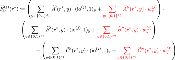
  The terms that depend solely on the instance and common input can be computed by the verifier locally. The remaining terms that depend on the witness, highlighted in above, are terms that the prover needs to send to the verifier. We denote these terms by $\lbrace \nu ^{(j)}_{A,2}, \nu ^{(j)}_{B,2}, \nu ^{(j)}_{C,2} \rbrace _{j \in [k]}$, where for each $j \in [k]$,

  

  There are two crucial observations to be made here: (i) for each fixed $r^*$, the above values are simply a linear combination of each individual witness $w^{(j)}$ (with appropriate coefficients); and (ii) the linear coefficients are the same for each witness, and in fact the linear coefficients depend only on the index of the witness.

• 4. The above observations allow the prover to open the commitments to $\lbrace \nu ^{(j)}_{A,2}, \nu ^{(j)}_{B,2}, \nu ^{(j)}_{C,2} \rbrace _{j \in [k]}$ by the linear homomorphism property of $\mathsf {LHC}$ since the property allows for the same linear coefficient to be applied all values in the k-tuple within the commitment.

  Specifically, the prover sends the values (and randomness) in the clear to the verifier, who then performs the same linear homomorphism over the committed values $\left\{ c_y \right\} _{y \in [|w|]}$ to check if the openings sent by the prover are correct before computing the checks necessitated by the sumcheck. While we remarked that the values that are inside the commitment are binary, this is not true of the linear coefficients that are in $\mathbb {F}$. But since $\mathbb {F}= \mathbb {F}_2[\alpha ]/(v(\alpha ))$, by the homomorphism with respect to polynomial property of $\mathsf {LHC}$ and that $\mathbb {F}_2[\alpha ]/(v(\alpha )) \subset \mathbb {Z}[\alpha ]/(v(\alpha ))$, it is fine that coefficients are in $\mathbb {F}$.

  Lastly it should be noted that the homomorphism properties are defined over $\mathbb {Z}[\alpha ]/(v(\alpha ))$ and not $\mathbb {F}_2[\alpha ]/(v(\alpha ))$, meaning there is no modular reduction in the coefficients of the resultant polynomial after the homomorphism operation, i.e. the length vector has elements in $\mathbb {Z}$ instead of $\mathbb {F}_2$. Therefore, to verify correctness of the commitment, the prover computes the values $\lbrace \nu ^{(j)}_{A,2}, \nu ^{(j)}_{B,2}, \nu ^{(j)}_{C,2} \rbrace _{j \in [k]}$ over $\mathbb {Z}[\alpha ]/(v(\alpha ))$, i.e. no modular reduction. The verifier does the commitment check over $\mathbb {Z}[\alpha ]/(v(\alpha ))$, but once the check passes successfully reduces to $\mathbb {F}_2[\alpha ]/(v(\alpha ))$¹³. While this increases the number of bits sent by the prover, we show in the full version of the paper that the increase is quite small, giving us the following theorem.

Theorem 4

Assuming the existence of somewhere-extractable linearly homomorphic commitments, the protocol in Fig. 2 is a dual-mode interactive batch argument for $\mathsf {R1CS}$ where

• Total communication cost is $O(m\lambda + (\lambda + k)\log m)$

• The verifier’s total run time is

where all instances have the same length $|\text {io}|$.

We defer the proof to the full version of the paper. Since we start with Boolean circuit satisfiability to generate $\mathsf {R1CS}$ instances, we get the following corollary with costs corresponding to the size the Boolean circuit.

Corollary 1

If we start with ${\mathsf {C}\text {-}\mathsf {SAT}}$ instances defined by a boolean circuit $C:\{0,1\}^{|x|} \times \{0,1\}^{|y|} \mapsto \{0,1\}$, then the protocol in Fig. 2 is a dual-mode interactive batch argument for ${\mathsf {C}\text {-}\mathsf {SAT}}$ where

• Total communication cost is

• The verifier’s total run time is

6 Non-interactive Batch Arguments for $\mathsf {NP}$

We now construct a non-interactive batch argument system for $\mathsf {NP}$. We start by formally defining this notion below.

Definition 4 (Non-interactive Batch Arguments)

A non-interactive batch argument for an $\mathsf {NP}$ language $L$ defined by relation $\mathcal {R}_{L}$ is a tuple of algorithms $(\mathsf {Gen},\mathsf {P},\mathsf {V})$ satisfying the following properties:

• Completeness: For all $\mathbf {x}=(x_1,\ldots ,x_k)$ and $\mathbf {w}=(w_1,\ldots ,w_k)$ such that for each $i\in [k]$, $\mathcal {R}_{L}(x_i,w_i)=1$, it holds that:

  

• (Non-adaptive) Soundness: For every PPT adversary $\mathsf {P}^*$ and all $\mathbf {x}=(x_1,\ldots ,x_k)$ where $\exists i$ s.t. $x_i\notin L$, it holds that:

  

In the full version, we show that the Fiat-Shamir transform w.r.t. $\mathcal {H}$ when applied to any strongly $\mathsf {FS}$ compatible protocol is sound as long as $\mathcal {H}$ is correlation intractable for $\mathsf {TC}^0$. Next, we construct a non-interactive batch argument system for $\mathsf {NP}$ by demonstrating that the above transformation remains sound when applied to our dual-mode interactive batch argument (Sect. 5), even though the aforementioned protocol does not satisfy strong $\mathsf {FS}$ compatibility. Finally, we show that we show that although our described protocol has a linear dependence on k, this can be made sub-linear.

References

Barak, B.: How to go beyond the black-box simulation barrier. In: 42nd FOCS, pp. 106–115. IEEE Computer Society Press, October 2001
Bartusek, J., Bronfman, L., Holmgren, J., Ma, F., Rothblum, R.D.: On the (in)security of Kilian-based SNARGs. In: Hofheinz, D., Rosen, A. (eds.) TCC 2019, Part II. LNCS, vol. 11892, pp. 522–551. Springer, Cham (2019). https://doi.org/10.1007/978-3-030-36033-7_20
Bitansky, N., Canetti, R., Chiesa, A., Tromer, E.: From extractable collision resistance to succinct non-interactive arguments of knowledge, and back again. In: Goldwasser, S. (ed.) ITCS 2012, pp. 326–349. ACM, January 2012
Bitansky, N., Canetti, R., Chiesa, A., Tromer, E.: Recursive composition and bootstrapping for SNARKS and proof-carrying data. In: Boneh, D., Roughgarden, T., Feigenbaum, J. (eds.) 45th ACM STOC, pp. 111–120. ACM Press, June 2013
Brakerski, Z., Goldwasser, S.: Circular and leakage resilient public-key encryption under subgroup indistinguishability - (or: Quadratic Residuosity Strikes Back). In: Rabin, T. (ed.) CRYPTO 2010. LNCS, vol. 6223, pp. 1–20. Springer, Heidelberg (2010). https://doi.org/10.1007/978-3-642-14623-7_1
Brakerski, Z., Holmgren, J., Kalai, Y.T.: Non-interactive delegation and batch NP verification from standard computational assumptions. In: Hatami, H., McKenzie, P., King, V. (eds.) 49th ACM STOC, pp. 474–482. ACM Press, June 2017
Brakerski, Z., Koppula, V., Mour, T.: NIZK from LPN and trapdoor hash via correlation intractability for approximable relations. In: Micciancio, D., Ristenpart, T. (eds.) CRYPTO 2020, Part III. LNCS, vol. 12172, pp. 738–767. Springer, Cham (2020). https://doi.org/10.1007/978-3-030-56877-1_26
Brakerski, Z., Lombardi, A., Segev, G., Vaikuntanathan, V.: Anonymous IBE, leakage resilience and circular security from new assumptions. In: Nielsen, J.B., Rijmen, V. (eds.) EUROCRYPT 2018, Part I. LNCS, vol. 10820, pp. 535–564. Springer, Cham (2018). https://doi.org/10.1007/978-3-319-78381-9_20
Camenisch, J., Hohenberger, S., Pedersen, M.Ø.: Batch verification of short signatures. J. Cryptol. 25(4), 723–747 (2012)
Canetti, R., et al.: Fiat-Shamir: from practice to theory. In: Charikar, M., Cohen, E. (eds.) 51st ACM STOC, pp. 1082–1090. ACM Press, June 2019
Canetti, R., Chen, Y., Reyzin, L., Rothblum, R.D.: Fiat-Shamir and correlation intractability from strong KDM-secure encryption. In: Nielsen, J.B., Rijmen, V. (eds.) EUROCRYPT 2018, Part I. LNCS, vol. 10820, pp. 91–122. Springer, Cham (2018). https://doi.org/10.1007/978-3-319-78381-9_4
Canetti, R., Goldreich, O., Halevi, S.: The random oracle methodology, revisited. J. ACM 51(4), 557–594 (2004)
Chor, B., Goldreich, O., Kushilevitz, E., Sudan, M.: Private information retrieval. In: 36th FOCS, pp. 41–50. IEEE Computer Society Press, October 1995
Choudhuri, A.R., Hubácek, P., Kamath, C., Pietrzak, K., Rosen, A., Rothblum, G.N.: Finding a Nash equilibrium is no easier than breaking Fiat-Shamir. In: Charikar, M., Cohen, E. (eds.) 51st ACM STOC, pp. 1103–1114. ACM Press, June 2019
Choudhuri, A.R., Jain, A., Jin, Z.: Non-interactive batch arguments for np from standard assumptions. Cryptology ePrint Archive, Report 2021/807 (2021). https://eprint.iacr.org/2021/807
Ciampi, M., Parisella, R., Venturi, D.: On adaptive security of delayed-input sigma protocols and Fiat-Shamir NIZKs. In: Galdi, C., Kolesnikov, V. (eds.) SCN 2020. LNCS, vol. 12238, pp. 670–690. Springer, Cham (2020). https://doi.org/10.1007/978-3-030-57990-6_33
Couteau, G., Katsumata, S., Ursu, B.: Non-interactive zero-knowledge in pairing-free groups from weaker assumptions. In: Canteaut, A., Ishai, Y. (eds.) EUROCRYPT 2020, Part III. LNCS, vol. 12107, pp. 442–471. Springer, Cham (2020). https://doi.org/10.1007/978-3-030-45727-3_15
Damgård, I., Faust, S., Hazay, C.: Secure two-party computation with low communication. In: Cramer, R. (ed.) TCC 2012. LNCS, vol. 7194, pp. 54–74. Springer, Heidelberg (2012). https://doi.org/10.1007/978-3-642-28914-9_4
Döttling, N., Garg, S.: Identity-based encryption from the Diffie-Hellman assumption. In: Katz, J., Shacham, H. (eds.) CRYPTO 2017, Part I. LNCS, vol. 10401, pp. 537–569. Springer, Cham (2017). https://doi.org/10.1007/978-3-319-63688-7_18
Döttling, N., Garg, S., Hajiabadi, M., Masny, D.: New constructions of identity-based and key-dependent message secure encryption schemes. In: Abdalla, M., Dahab, R. (eds.) PKC 2018, Part I. LNCS, vol. 10769, pp. 3–31. Springer, Cham (2018). https://doi.org/10.1007/978-3-319-76578-5_1
Döttling, N., Garg, S., Ishai, Y., Malavolta, G., Mour, T., Ostrovsky, R.: Trapdoor hash functions and their applications. In: Boldyreva, A., Micciancio, D. (eds.) CRYPTO 2019, Part III. LNCS, vol. 11694, pp. 3–32. Springer, Cham (2019). https://doi.org/10.1007/978-3-030-26954-8_1
Fiat, A., Shamir, A.: How to prove yourself: practical solutions to identification and signature problems. In: Odlyzko, A.M. (ed.) CRYPTO 1986. LNCS, vol. 263, pp. 186–194. Springer, Heidelberg (1987). https://doi.org/10.1007/3-540-47721-7_12
Garg, S., Hajiabadi, M.: Trapdoor functions from the computational Diffie-Hellman assumption. In: Shacham, H., Boldyreva, A. (eds.) CRYPTO 2018, Part II. LNCS, vol. 10992, pp. 362–391. Springer, Cham (2018). https://doi.org/10.1007/978-3-319-96881-0_13
Gentry, C., Wichs, D.: Separating succinct non-interactive arguments from all falsifiable assumptions. In: Fortnow, L., Vadhan, S.P. (eds.) 43rd ACM STOC, pp. 99–108. ACM Press, June 2011
Goldreich, O., Håstad, J.: On the complexity of interactive proofs with bounded communication. Inf. Process. Lett. 67(4), 205–214 (1998)
Goldreich, O., Vadhan, S.P., Wigderson, A.: On interactive proofs with a laconic prover. Comput. Complex. 11(1–2), 1–53 (2002)
Goldwasser, S., Kalai, Y.T.: On the (in)security of the Fiat-Shamir paradigm. In: 44th FOCS, pp. 102–115. IEEE Computer Society Press, October 2003
Goldwasser, S., Lin, H., Rubinstein, A.: Delegation of computation without rejection problem from designated verifier CS-Proofs. Cryptology ePrint Archive, Report 2011/456 (2011). http://eprint.iacr.org/2011/456
Holmgren, J., Lombardi, A.: Cryptographic hashing from strong one-way functions (or: One-way product functions and their applications). In: Thorup, M. (ed.) 59th FOCS, pp. 850–858. IEEE Computer Society Press, October 2018
Hubacek, P., Wichs, D.: On the communication complexity of secure function evaluation with long output. In: Roughgarden, T. (ed.) ITCS 2015, pp. 163–172. ACM, January 2015
Jain, A., Jin, Z.: Non-interactive zero knowledge from sub-exponential DDH. In: Canteaut, A., Standaert, F.-X. (eds.) EUROCRYPT 2021. LNCS, vol. 12696, pp. 3–32. Springer, Cham (2021). https://doi.org/10.1007/978-3-030-77870-5_1
Jawale, R., Kalai, Y.T., Khurana, D., Zhang, R.: SNARGs for bounded depth computations and PPAD hardness from sub-exponential LWE. In: STOC. ACM (2021)
Jawale, R., Khurana, D.: Lossy correlation intractability and PPAD hardness from sub-exponential LWE. Cryptology ePrint Archive, Report 2020/911 (2020). https://eprint.iacr.org/2020/911
Kalai, Y.T., Paneth, O., Yang, L.: How to delegate computations publicly. In: Charikar, M., Cohen, E. (eds.) 51st ACM STOC, pp. 1115–1124. ACM Press, June 2019
Kalai, Y.T., Rothblum, G.N., Rothblum, R.D.: From obfuscation to the security of Fiat-Shamir for proofs. In: Katz, J., Shacham, H. (eds.) CRYPTO 2017, Part II. LNCS, vol. 10402, pp. 224–251. Springer, Cham (2017). https://doi.org/10.1007/978-3-319-63715-0_8
Kalai, Y.T., Zhang, R.: SNARGs for bounded depth computations from sub-exponential LWE. Cryptology ePrint Archive, Report 2020/860 (2020). https://eprint.iacr.org/2020/860
Kaslasi, I., Rothblum, G.N., Rothblum, R.D., Sealfon, A., Vasudevan, P.N.: Batch verification for statistical zero knowledge proofs. In: Pass, R., Pietrzak, K. (eds.) TCC 2020, Part II. LNCS, vol. 12551, pp. 139–167. Springer, Cham (2020). https://doi.org/10.1007/978-3-030-64378-2_6
Kaslasi, I., Rothblum, R.D., Vasudevanr, P.N.: Public-coin statistical zero-knowledge batch verification against malicious verifiers. In: Canteaut, A., Standaert, F.-X. (eds.) EUROCRYPT 2021. LNCS, vol. 12698, pp. 219–246. Springer, Cham (2021). https://doi.org/10.1007/978-3-030-77883-5_8
Kilian, J.: A note on efficient zero-knowledge proofs and arguments (extended abstract). In: 24th ACM STOC, pp. 723–732. ACM Press, May 1992
Koppula, V., Lewko, A.B., Waters, B.: Indistinguishability obfuscation for turing machines with unbounded memory. In: Servedio, R.A., Rubinfeld, R. (eds.) 47th ACM STOC, pp. 419–428. ACM Press, June 2015
Kushilevitz, E., Ostrovsky, R.: Replication is NOT needed: SINGLE database, computationally-private information retrieval. In: 38th FOCS, pp. 364–373. IEEE Computer Society Press, October 1997
Lombardi, A., Vaikuntanathan, V.: Fiat-Shamir for repeated squaring with applications to PPAD-hardness and VDFs. In: Micciancio, D., Ristenpart, T. (eds.) CRYPTO 2020, Part III. LNCS, vol. 12172, pp. 632–651. Springer, Cham (2020). https://doi.org/10.1007/978-3-030-56877-1_22
Lund, C., Fortnow, L., Karloff, H.J., Nisan, N.: Algebraic methods for interactive proof systems. J. ACM 39(4), 859–868 (1992)
Micali, S.: CS proofs (extended abstracts). In: 35th FOCS, pp. 436–453. IEEE Computer Society Press, November 1994
Naor, M.: On cryptographic assumptions and challenges (invited talk). In: Boneh, D. (ed.) CRYPTO 2003. LNCS, vol. 2729, pp. 96–109. Springer, Heidelberg (2003). https://doi.org/10.1007/978-3-540-45146-4_6
Okamoto, T., Pietrzak, K., Waters, B., Wichs, D.: New realizations of somewhere statistically binding hashing and positional accumulators. In: Iwata, T., Cheon, J.H. (eds.) ASIACRYPT 2015, Part I. LNCS, vol. 9452, pp. 121–145. Springer, Heidelberg (2015). https://doi.org/10.1007/978-3-662-48797-6_6
Peikert, C., Shiehian, S.: Noninteractive zero knowledge for NP from (Plain) learning with errors. In: Boldyreva, A., Micciancio, D. (eds.) CRYPTO 2019, Part I. LNCS, vol. 11692, pp. 89–114. Springer, Cham (2019). https://doi.org/10.1007/978-3-030-26948-7_4
Reingold, O., Rothblum, G.N., Rothblum, R.D.: Constant-round interactive proofs for delegating computation. In: Wichs, D., Mansour, Y. (eds.) 48th ACM STOC, pp. 49–62. ACM Press, June 2016
Reingold, O., Rothblum, G.N., Rothblum, R.D.: Efficient batch verification for UP. In: Computational Complexity Conference. LIPIcs, vol. 102, pp. 22:1–22:23. Schloss Dagstuhl - Leibniz-Zentrum für Informatik (2018)
Rothblum, G.N., Rothblum, R.D.: Batch verification and proofs of proximity with polylog overhead. In: Pass, R., Pietrzak, K. (eds.) TCC 2020, Part II. LNCS, vol. 12551, pp. 108–138. Springer, Cham (2020). https://doi.org/10.1007/978-3-030-64378-2_5
Setty, S.: Spartan: efficient and general-purpose zkSNARKs without trusted setup. In: Micciancio, D., Ristenpart, T. (eds.) CRYPTO 2020, Part III. LNCS, vol. 12172, pp. 704–737. Springer, Cham (2020). https://doi.org/10.1007/978-3-030-56877-1_25
Shamir, A.: IP = PSPACE. J. ACM 39(4), 869–877 (1992)
Acknowledgments
Arka Rai Choudhuri, Abhishek Jain and Zhengzhong Jin are supported in part by NSF CNS-1814919, NSF CAREER 1942789 and Johns Hopkins University Catalyst award. Arka Rai Choudhuri and Abhishek Jain are also supported in part by the Office of Naval Research Grant N00014-19-1-2294. Arka Rai Choudhuri is also supported in part by NSF Grant CNS-1908181. Zhengzhong Jin is also supported in part by NSF CAREER 1845349.
Author information
Authors and Affiliations
Corresponding author
Editor information
Editors and Affiliations
Rights and permissions
Copyright information
© 2021 International Association for Cryptologic Research
About this paper
Cite this paper
Choudhuri, A.R., Jain, A., Jin, Z. (2021). Non-interactive Batch Arguments for NP from Standard Assumptions. In: Malkin, T., Peikert, C. (eds) Advances in Cryptology – CRYPTO 2021. CRYPTO 2021. Lecture Notes in Computer Science(), vol 12828. Springer, Cham. https://doi.org/10.1007/978-3-030-84259-8_14
Download citation
DOI: https://doi.org/10.1007/978-3-030-84259-8_14
Published:
Publisher Name: Springer, Cham
Print ISBN: 978-3-030-84258-1
Online ISBN: 978-3-030-84259-8
eBook Packages: Computer ScienceComputer Science (R0)