Fully Succinct Batch Arguments for $\textsf{NP}$ from Indistinguishability Obfuscation

Abstract

Non-interactive batch arguments for $\textsf{NP}$ provide a way to amortize the cost of $\textsf{NP}$ verification across multiple instances. In particular, they allow a prover to convince a verifier of multiple $\textsf{NP}$ statements with communication that scales sublinearly in the number of instances.

   In this work, we study fully succinct batch arguments for $\textsf{NP}$ in the common reference string (CRS) model where the length of the proof scales not only sublinearly in the number of instances T, but also sublinearly with the size of the $\textsf{NP}$ relation. Batch arguments with these properties are special cases of succinct non-interactive arguments (SNARGs); however, existing constructions of SNARGs either rely on idealized models or strong non-falsifiable assumptions. The one exception is the Sahai-Waters SNARG based on indistinguishability obfuscation. However, when applied to the setting of batch arguments, we must impose an a priori bound on the number of instances. Moreover, the size of the common reference string scales linearly with the number of instances.

   In this work, we give a direct construction of a fully succinct batch argument for $\textsf{NP}$ that supports an unbounded number of statements from indistinguishability obfuscation and one-way functions. Then, by additionally relying on a somewhere statistically-binding (SSB) hash function, we show how to extend our construction to obtain a fully succinct and updatable batch argument. In the updatable setting, a prover can take a proof $\pi$ on T statements $(x_1, \ldots , x_T)$ and “update” it to obtain a proof $\pi '$ on $(x_1, \ldots , x_T, x_{T + 1})$. Notably, the update procedure only requires knowledge of a (short) proof for $(x_1, \ldots , x_T)$ along with a single witness $w_{T + 1}$ for the new instance $x_{T + 1}$. Importantly, the update does not require knowledge of witnesses for $x_1, \ldots , x_T$.

1 Introduction

Non-interactive batch arguments (BARGs) provide a way to amortize the cost of $\textsf{NP}$ verification across multiple instances. Specifically, in a batch argument, the prover has a collection of $\textsf{NP}$ statements $x_1, \ldots , x_T$ and their goal is to convince the verifier that $x_i \in \mathcal {L}$ for all i, where $\mathcal {L}$ is the associated $\textsf{NP}$ language. The trivial solution is to have the prover send over the associated $\textsf{NP}$ witnesses $w_1, \ldots , w_T$ and have the verifier check each one individually. The goal in a batch argument is to obtain shorter proofs—namely, proofs whose size scales sublinearly in T.

In this work, we operate in the common reference string (CRS) model where we assume that there is a one-time (trusted) sampling of a structured reference string. Within this model, we focus on the setting where where the proof is non-interactive (i.e., the proof consists of a single message from the prover to the verifier) and publicly-verifiable (i.e., verifying the proof only requires knowledge of the associated statements and the CRS). Finally, we require soundness to hold against computationally-bounded provers; namely, our goal is to construct batch argument systems. Recently, there has been a flurry of work constructing batch arguments for $\textsf{NP}$ satisfying these requirements from standard lattice assumptions [CJJ21b, DGKV22], assumptions on groups with bilinear maps [WW22], and from a combination of subexponential hardness of the DDH assumption together with the QR assumption [CJJ21a].

This work: fully succinct batch arguments. The size of the proof in the aforementioned BARG constructions all scale linearly with the size of the $\textsf{NP}$ relation. In other words, to check T statements for an $\textsf{NP}$ relation that is computable by a circuit of size s, the proof sizes scale with $\textsf{poly} (\lambda , s) \cdot o(T)$, where $\lambda$ is the security parameter. In this work, we study the setting where the proof $\pi$ scales sublinearly in both the number of instances T and the size s of the $\textsf{NP}$ relation. More precisely, we require that $|\pi | = \textsf{poly} (\lambda , \log s, \log T)$, and we refer to batch arguments satisfying this property to be “fully succinct.” Our primary goal in this work is to minimize the communication cost (and in conjunction, the verifier cost) of batch $\textsf{NP}$ verification.

We note that this level of succinctness is typically characteristic of succinct non-interactive arguments (SNARGs), and indeed any SNARG directly implies a fully succinct batch argument. However, existing constructions of SNARGs either rely on random oracles [Mic95, BBHR18, COS20, CHM+20, Set20], the generic group model [Gro16], or strong non-falsifiable assumptions [Gro10, BCCT12, DFH12, Lip13, PHGR13, GGPR13, BCI+13, BCPR14, BISW17, BCC+17, BISW18, ACL+22]. Indeed, Gentry and Wichs [GW11] showed that no construction of an (adaptively-sound) SNARG for $\textsf{NP}$ can be proven secure via a black-box reduction to a falsifiable assumption [Nao03].

The only construction of (non-adaptively sound) SNARGs from falsifiable assumptions is the construction by Sahai and Waters based on indistinguishability obfuscation ($i\mathcal {O}$) [SW14] in conjunction with the recent breakthrough works of Jain et al.  [JLS21, JLS22] that base indistinguishability obfuscation on falsifiable assumptions. However, the Sahai-Waters SNARG from $i\mathcal {O}$ imposes an a priori bound on the number of statements that can be proven, and in particular, the size of the CRS grows with the total length of the statement and witness (i.e., the CRS consists of an obfuscated program that reads in the statement and the witness and outputs a signature on the statements if the input is well-formed). When applied to the setting of batch verification, this limitation means that we need to impose an a priori bound of the number of instances that can be proved, and the size of the CRS necessarily scales with this bound. Our goal in this work is to construct a fully succinct batch argument for $\textsf{NP}$ that supports an arbitrary number of instances from indistinguishability obfuscation and one-way functions (i.e., the same assumption as the construction of Sahai and Waters).

An approach using recursive composition. A natural approach to constructing a fully succinct batch argument that supports an arbitrary polynomial number of statements is to compose a SNARG with polylogarithmic verification cost (for a single statement) with a batch argument that supports an unbounded number of statements. Namely, to prove that $(x_1, \ldots , x_T)$ are true, the prover would proceed as follows:

• 1. First, for each statement $x_i \in \{0,1\}^\ell$, the prover constructs a SNARG proof $\pi _i$. If the SNARG has a polylogarithmic verification procedure, then the size of the SNARG verification circuit for checking $(x_i, \pi _i)$ is bounded by $\textsf{poly} (\lambda , \ell , \log s)$, where s is the size of the circuit for checking the underlying $\textsf{NP}$ relation.

• 2. Next, the prover uses a batch argument to demonstrate that it knows $(\pi _1, \ldots , \pi _T)$ where $\pi _i$ is an accepting SNARG proof on instance $x_i \in \{0,1\}^\ell$. This is a batch argument for checking T instances of the SNARG verification circuit, which has size $\textsf{poly} (\lambda , \ell , \log s)$. If the size of the batch argument scales polylogarithmically with the number of instances, then the overall proof has size $\textsf{poly} (\lambda , \ell , \log s, \log T)$.

Moreover, using a somewhere extractable commitment scheme [HW15, CJJ21b], it is possible to remove the dependence on the instance size $\ell$.¹ This yields a fully succinct batch argument with proof size $\textsf{poly} (\lambda , \log s, \log T)$. To argue (non-adaptive) soundness of this approach, we rely on soundness of the underlying SNARG and somewhere extractability of the underlying batch argument (i.e., a BARG where the CRS can be programmed to a specific (hidden) index $i^*$ such that there exists an efficient extractor that takes any accepting proof $\pi$ for a tuple $(x_1, \ldots , x_T)$ and outputs a valid witness $w_{i^*}$ for instance $x_{i^*}$). We can now instantiate the SNARG with polylogarithmic verification cost using the Sahai-Waters construction based on $i\mathcal {O}$ and one-way functions, and the somewhere extractable BARG for an unbounded number of instances with the recent lattice-based scheme of Choudhuri et al.  [CJJ21b]. This result provides a basic feasibility result for the existence of fully succinct batch arguments for $\textsf{NP}$. However, instantiating this compiler requires two sets of assumptions: $i\mathcal {O}$ and one-way functions for the underlying SNARG, and lattice-based assumptions for the BARG.

This work. In this work, we provide a direct route for constructing fully succinct BARGs that support an unbounded number of statements from $i\mathcal {O}$ and one-way functions. Notably, combined with the breakthrough work of Jain, Lin, and Sahai [JLS22], this provides an instantiation of fully succinct BARGs without lattice assumptions (in contrast to the generic approach above). Using our construction, proving T statements for an $\textsf{NP}$ relation of size s requires a proof of length $\textsf{poly} (\lambda )$. This is independent of both the number of statements T and the size s of the associated $\textsf{NP}$ relation. Like the scheme of Sahai and Waters, our construction satisfies non-adaptive soundness (and perfect zero-knowledge). We summarize this instantiation in the informal theorem below:

Theorem 1.1

(Fully Succinct BARG (Informal)). Assuming the existence of indistinguishability obfuscation and one-way functions, there exists a fully succinct, non-adaptively sound batch argument for $\textsf{NP}$. The batch argument satisfies perfect zero knowledge.

Updatable batch arguments. We also show how to extend our construction to obtain an updatable BARG through the use of somewhere statistically binding (SSB) hash functions [HW15, OPWW15]. In an updatable BARG, a prover is able to take an existing proof $\pi _T$ on statements $(x_1,\ldots ,x_T)$ along with a new statement $x_{T+1}$ with associated $\textsf{NP}$ witness $w_{T+1}$ and update $\pi$ to a new proof $\pi '$ on instances $(x_1,\ldots ,x_T,x_{T+1})$. Notably, the update algorithm does not require the prover to have a witness for any statement other than $x_{T+1}$. This is useful in settings where the full set of statements/witnesses are not fixed in advance (e.g., in a streaming setting). For example, a prover might want to compute a summary of all transactions that occur in a given day and then provide a proof that the summary reflects the complete set of transactions from the day. An updatable BARG would allow the prover to maintain just a single proof that authenticates all of the summary reports from different days, and moreover, the prover does not have to maintain the full list of transactions from earlier days to perform the update. We show how to obtain a fully succinct updatable BARG in Sect. 5, and we summarize this instantiation in the following theorem.

Theorem 1.2

(Updatable BARG (Informal)). Assuming the existence of indistinguishability obfuscation scheme and somewhere statistical binding hash functions, there exists a fully succinct, non-adaptively sound updatable batch argument for $\textsf{NP}$. The batch argument satisfies perfect zero knowledge.

1.1 Technical Overview

In this section, we provide an informal overview of the techniques that we use to construct fully succinct BARGs. Throughout this section, we consider the batch $\textsf{NP}$ language of Boolean circuit satisfiability. Namely, the prover has a Boolean circuit C and a collection of instances $x_1, \ldots , x_T$, and its goal is to convince the verifier that there exist witnesses $w_1, \ldots , w_T$ such that $C(x_i, w_i) = 1$ for all $i \in [T]$.

The Sahai-Waters SNARG. As a warmup, we recall the Sahai-Waters [SW14] construction of SNARGs from $i\mathcal {O}$ for a single instance (i.e., the case where $T = 1$). In this construction, the common reference string (CRS) consists of two obfuscated programs: $\textsf{Prove}$ and $\textsf{Verify}$. The $\textsf{Prove}$ program takes in the circuit C, the statement x, and the witness w, and outputs a signature $\sigma _x$ on x if $C(x, w) = 1$ and $\bot$ otherwise. The proof is simply the signature $\pi = \sigma _x$. The $\textsf{Verify}$ program takes in the description of the circuit C, the statement x, and the proof $\pi = \sigma _x$ and checks whether $\sigma _x$ is a valid signature on x or not. The signature in this case just corresponds to the evaluation of a pseudorandom function (PRF) on the input x. The key to the PRF is hard-coded in the obfuscated proving and verification programs. Security in turn, relies on the Sahai-Waters “punctured programming” technique.

Batch arguments for index languages. To construct fully succinct batch arguments, we start by considering the special case of an index language (similar to the starting point in the lattice-based construction of Choudhuri et al.  [CJJ21b]). In a BARG for an index language, the statements are simply the indices $(1, 2, \ldots , T)$. The prover’s goal is to convince the verifier that there exists $w_i$ such that $C(i, w_i) = 1$ for all $i \in [T]$. We start by showing how to construct a fully succinct BARG for index languages with an unbounded number of instances (i.e., an index language for arbitrary polynomial T). Our construction proceeds iteratively as follows. Like the Sahai-Waters construction, the CRS in our scheme consists of the obfuscation of the following two programs:

• The proving program takes in a circuit C, an index i, a witness $w_i$ for instance i and a proof $\pi$ for the first $i-1$ statements. The program checks if $C(i,w_i)=1$ and that the proof on the first $i-1$ statements is valid. When $i=1$, then we ignore the latter check. If both conditions are satisfied, the program outputs a signature on statement (C, i). Notably, the size of the prover program only scales with the size of the circuit and the bit-length of the number of instances (instead of linearly with the number of instances). Similar to the construction of Sahai and Waters, we define the “signature” on the statement (C, i) to be $\pi = \textsf{F}(k, (C, i))$, where $\textsf{F}$ is a puncturable PRF [BW13, KPTZ13, BGI14],² and k is a PRF key that is hard-coded in the proving program.

• To verify a proof on T statements (i.e., the instances $1, \ldots , T$), the verification program simply checks that the proof $\pi$ is a valid signature on the pair (C, T). Based on how we defined the proving program above, this corresponds to checking that $\pi = \textsf{F}(k, (C, T))$. Now, to argue soundness using the Sahai-Waters punctured programming paradigm, we modify this check and replace it with the check

  

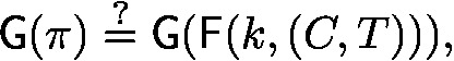
  where $\textsf{G}$ is a length-doubling pseudorandom generator. This will be critical for arguing soundness.

Soundness of the index BARG. To argue non-adaptive soundness of the above approach (i.e., the setting where the statement is chosen independently of the CRS), we apply the punctured programming techniques of Sahai and Waters [SW14]. Take any circuit $C^*$ and suppose there is an index $i^*$ where for all witnesses w, we have that $C^* (i^*, w) = 0$. Our soundness analysis proceeds in two steps:

• We first show that no efficient prover can compute an accepting proof $\pi$ on instances $(1, \ldots , i^*)$ for circuit $C^*$.

• Then, we show how to “propagate” the inability to construct a valid proof on index $i^*$ to all indices $i \ge i^*$. This in turn suffices to argue non-adaptive soundness for an arbitrary polynomial number of statements.

We now sketch the argument for the first step. In the following overview, suppose the output space of $\textsf{F}$ is $\{0,1\}^\lambda$ and suppose that $\textsf{G}:\{0,1\}^\lambda \rightarrow \{0,1\}^{2 \lambda }$ is length-doubling.

• The real CRS consists of obfuscations of the following proving and verification programs:

  

• First, instead of embedding the real PRF key k in the proving and verification programs, we embed a punctured PRF key $k'$ that is punctured on the input $(C^*, i^*)$. Whenever the proving and verification program needs to evaluate $\textsf{F}$ on the punctured point $(C^*, i^*)$, we hard-code the value $z = \textsf{F}(k, (C^*, i^*))$:

  

  Since the punctured PRF is functionality-preserving, on all inputs $(C, i) \ne (C^*, i^*)$, we have that $\textsf{F}(k, (C, i)) = \textsf{F}(k', (C, i))$. Since $z = \textsf{F}(k, (C^*, i^*))$, the input/output behavior of the verification program is unchanged. Next, $C(i^*, w) = 0$ for all w, so the input/output behavior of the proving program is also unchanged. Security of $i\mathcal {O}$ then ensures that the obfuscated proving and verification programs are computationally indistinguishable from those in the real scheme.

• Observe that both the proving and verification programs can be constructed given just the value of $\textsf{G}(z)$ without necessarily knowing z itself. We now replace the target value $\textsf{G}(z)$ with a uniform random string . This follows by (1) puncturing security of $\textsf{F}$ which says that the value of $z = \textsf{F}(k, (C^*, i^*))$ is computationally indistinguishable from a uniform string ; and (2) by PRG security since the distribution of $\textsf{G}(z)$ where is computationally indistinguishable from sampling a uniform random string . With these modifications, the proving and verification programs behave as follows:

  

• Since t is uniform in $\{0,1\}^{2\lambda }$, the probability that t is even in the image of $\textsf{G}$ is at most $2^{-\lambda }$. Thus, in this experiment, with probability $1 - 2^{-\lambda }$, there does not exist any accepting proof $\pi$ for input $(C^*, i^*)$. This means that we can now revert to using the PRF key k in both the proving and verification programs and simply reject all proofs on instance $(C^*, i^*)$. In other words, we can replace the proving and verification programs with obfuscations of the following programs by appealing to the security of $i\mathcal {O}$:

  

In this final experiment, there no longer exists an accepting proof $\pi$ on instances $(1, \ldots , i^*)$ for circuit $C^*$. Next, we show how to extend this argument to additionally remove accepting proofs on the batch of instances $(1, \ldots , i^*, i^*+ 1)$. We leverage a similar strategy as before:

• We replace the PRF key k with a punctured key $k'$ that is punctured at $(C^*, i^*+ 1)$ in both the proving and verification programs. Again, whenever the programs need to compute $\textsf{F}(k, (C^*, i^*+ 1))$, we substitute a hard-coded value $z = \textsf{F}(k, (C^*, i^*+ 1))$:

  

  Note that to simplify the notation, we merged the individual checks ($C = C^*$ and $i = i^*$) and ($C = C^*$ and $i - 1 = i^*$) in the proving program into a single check that outputs $\bot$ if satisfied.

• Observe once again that the description of the proving and verification programs only depends on $\textsf{G}(z)$ (and not z itself). By the same sequence of steps as above, we can appeal to puncturing security of $\textsf{F}$, pseudorandomness of $\textsf{G}$, and security of $i\mathcal {O}$ to show that the obfuscated proving and verification programs are computationally indistinguishable from the following programs:

  

We can repeat the above strategy any polynomial number of times. In particular, for any $T = \textsf{poly} (\lambda )$, we can replace the obfuscated programs in the CRS with the following programs:

By security of $i\mathcal {O}$, the puncturable PRF, and the PRG, this modified CRS is computationally indistinguishable from the real CRS. However, when the verification program is implemented as above, there are no accepting proofs on input $(C^*, i)$ for any $i^*\le i \le T$. Moreover, the size of the obfuscated programs only depends on $\log T$ (and not T). As such, the scheme supports an arbitrary polynomial number of statements. We give the full analysis in Sect. 3.

Adaptive soundness and zero knowledge. Using standard complexity leveraging techniques, we show how to extend our BARG for index languages with non-adaptive soundness into one with adaptive soundness in the full version of this paper. We note that due to the reliance on complexity leveraging, the resulting BARGs we obtain are no longer fully succinct; the proof size now scales with the size of the NP relation, but critically, still sublinearly in the number of instances. We also note that much like the construction of Sahai and Waters, both our fully succinct non-adaptive BARG and our adaptive BARG satisfy perfect zero-knowledge.

From index languages to general $\textsf{NP}$ languages. Next, we show how to bootstrap our fully succinct BARG for index languages to obtain a fully succinct BARG for $\textsf{NP}$ that supports an arbitrary polynomial number of statements. In this setting, the prover has a Boolean circuit C and arbitrary instances $x_1, \ldots , x_T$; the prover’s goal is to convince the verifier that for all $i \in [T]$, there exists $w_i$ such that $C(x_i, w_i) = 1$.

The key difference between general $\textsf{NP}$ languages and index languages is that the tuple of statements $(x_1, \ldots , x_T)$ no longer has a succinct description. This property was critical in our soundness analysis above. The soundness argument we described above works by embedding the instances $x_{i^*}, x_{i^*+ 1}, \ldots , x_T$ into the proving and verification programs (where $x_{i^*}$ denotes a false instance) and have the programs always reject proofs on these statements (with respect to the target circuit $C^*$). For index languages, these instances just correspond to the interval $[i^*+ 1, T]$, which can be described succinctly with $O(\log T)$ bits. When $x_{i^*}, x_{i^*+ 1}, \ldots , x_T$ are arbitrary instances, they do not have a short description, and we cannot embed these instances into the proving and verification programs without imposing an a priori bound on the number of instances.

Instead of modifying the above construction, we instead adopt the approach of Choudhuri et al.  [CJJ21b] who previously showed how to generically upgrade any BARG for index languages to a BARG for $\textsf{NP}$ by relying on somewhere extractable commitment schemes. If the underlying BARG for index languages supports an unbounded number of instances, then the transformed scheme also does. In our setting, we observe that if we only require (non-adaptive) soundness (as opposed to “somewhere extraction”), we can use a positional accumulator [KLW15] in place of the somewhere extractable commitment scheme. The advantage of basing the transformation on positional accumulators is that we can construct positional accumulators directly from indistinguishability obfuscation and one-way functions. Applied to the above index BARG construction (see also Sect. 3), we obtain a fully succinct batch argument for $\textsf{NP}$ from the same set of assumptions. In contrast, if we invoke the compiler of Choudhuri et al., we would need to additionally assume the existence of a somewhere extractable commitment scheme which cannot be based solely on indistinguishability obfuscation together with one-way functions in a fully black-box way [AS15].

Very briefly, in the Choudhuri et al. approach, to construct a batch argument on the tuple $(C, x_1, \ldots , x_T)$, the prover first computes a succinct hash y of the statements $(x_1, \ldots , x_T)$. Using y, they define an index relation where instance i is satisfied if there exists an opening $(x_i, \pi _i)$ to y at index i, and moreover, there exists a satisfying witness $w_i$ where $C(x_i, w_i) = 1$. The proof then consists of the hash y and a proof for the index relation. In this work, we show that using a positional accumulator to instantiate the hash function suffices to obtain a BARG with non-adaptive soundness. We provide the full details in Sect. 4.

Updatable BARGs for $\textsf{NP}$ . Our techniques also readily generalize to obtain an updatable batch argument (for general $\textsf{NP}$) from the same underlying set of assumptions. Recall that in an updatable BARG, a prover can take an existing proof $\pi$ on a tuple $(C, x_1, \ldots , x_T)$ together with a new statement $x_{T + 1}$ and witness $w_{T + 1}$ and extend $\pi$ to a new proof $\pi '$ on the tuple $(C, x_1, \ldots , x_T, x_{T + 1})$. One way to construct an updatable BARG is to recursive compose a succinct non-interactive argument of knowledge [BCCT13] or a rate-1 batch argument [DGKV22].³ Here, we opt for a more direct approach based on the above techniques, which does not rely on recursive composition.

First, our index BARG construction described above is already updatable. However, if we apply the Choudhuri et al.  [CJJ21b] transformation to obtain a BARG for $\textsf{NP}$, the resulting scheme is no longer updatable. This is because the transformation requires the prover to commit to the complete set of statements and then argue that the statement associated with each index is true (which in turn requires knowledge of all of the associated witnesses).

Instead, we take a different and more direct tree-based approach. For ease of exposition, suppose first that $T = 2^k$ for some integer k. Our construction will rely on a hash function H. Given a tuple of T statements $(x_1, \ldots , x_T)$, we construct a binary Merkle hash tree [Mer87] of depth k as follows: the leaves of the tree are labeled $x_1, \ldots , x_T$, and the value of each internal node v is the hash $H(v_1, v_2)$ of its two children $v_1$ and $v_2$. The output h of the hash tree is the value at the root node, and we denote this by writing $h = H_{\textsf{Merkle}}(x_1, \ldots , x_T)$. A proof on the tuple of instances $(x_1, \ldots , x_T)$ is simply a signature on the root node $H_{\textsf{Merkle}}(x_1, \ldots , x_T)$. Now, instead of providing an obfuscated program that takes a proof on index i and extends it into a proof on index $i + 1$, we define our obfuscated proving program to take in two signatures on hash values $h_1 = H_{\textsf{Merkle}}(x_1, \ldots , x_T)$ and $h_2 = H_{\textsf{Merkle}}(y_1, \ldots , y_T)$ and output a signature on the hash value $h = H(h_1, h_2) = H_{\textsf{Merkle}}(x_1, \ldots , x_T, y_1, \ldots , y_T)$. This new “two-to-one” obfuscated program allows us to merge two proofs on T instances into a single proof on 2T instances. More generally, the (obfuscated) proving program in the CRS now supports the following operations:

• Signing a single instance: Given a circuit C, a statement x, and a witness w, output a signature on (C, x, 1) if $C(x, w) = 1$ and $\bot$ otherwise. This can be viewed as a signature on a hash tree of depth 1.

• Merge trees: Given a circuit C, hashes $h_1, h_2$ associated with two trees of depth k, along with signatures $\sigma _1, \sigma _2$, check that $\sigma _1$ is a valid signature on $(C, h_1, k)$, and $\sigma _2$ is a valid signature on $(C, h_2, k)$. If both checks pass, output a signature on $(C, H(h_1, h_2), k + 1)$. This is a signature on a hash tree of depth $k + 1$.

To construct a proof on instances $(x_1, \ldots , x_T)$ using witnesses $(w_1, \ldots , w_T)$ for arbitrary T, we now proceed as follows:

• Run the (obfuscated) proving algorithm on $(C, x_1, w_1)$ to obtain a signature $\sigma$ on $(C, x_1, 1)$. The initial proof $\pi$ is simply the set $\{ (1, x_1, \sigma ) \}$.

• Suppose $\pi = \{ (i, h_i, \sigma _i) \}$ is a proof on the first $T - 1$ statements. To update the proof $\pi$ to a proof on the first T statements, first run the proving algorithm on $(C, x_T, w_T)$ to obtain a signature $\sigma$ on $(C, x_T, 1)$. Now, we apply the following merging procedure:

  • Initialize $(k, h', \sigma ') \leftarrow (1, x_T, \sigma )$ and $\pi ' \leftarrow \pi$.

  • While there exists $(i, h_i, \sigma _i) \in \pi '$ where $i = k$, run the (obfuscated) merge program on $(C, h_i, h', k, \sigma _i, \sigma ')$ to obtain a signature $\sigma ''$ on $(C, H(h_i, h'), k + 1)$. Remove $(i, h_i, \sigma _i)$ from $\pi '$ and update $(k, h', \sigma ') \leftarrow (k + 1, H(h_i, h'), \sigma '')$.

  • Add the tuple $(k, h', \sigma '')$ to $\pi '$ at the conclusion of the merging process.

  Observe that the update procedure only requires knowledge of the new statement $x_T$, its witness $w_T$, and the proof on the previous statements $\pi$; it does not require knowledge of the witnesses to the previous statements. Moreover, observe that the number of hash-signature tuples in $\pi$ is always bounded by $\log T$.

To verify a proof $\pi = \{ (i, h_i, \sigma _i) \}$ with respect to a Boolean circuit C, the verifier checks that $\sigma _i$ is a valid signature on $(C, h_i, i)$ for all tuples in $\pi$, and moreover, that each of the intermediate hash values $h_i$ are correctly computed from $(x_1, \ldots , x_T)$. Non-adaptive soundness of the above construction follows by a similar argument as that for our index BARG. Notably, we show that if an instance $x_{i^*}$ is false, then the proving program will never output a signature on input $(C, x_{i^*}, 1)$. Using the same punctured programming technique sketched above, we can again “propagate” the inability to compute a signature on the leaf node $i^*$ to argue that any efficient prover cannot compute a signature on any node that is an ancestor of $x_{i^*}$ in the hash tree. Here, we will need to rely on the underlying hash function being somewhere statistically binding [HW15, OPWW15]. By a hybrid argument, we can eventually move to an experiment where there are no accepting proofs on tuples that contain $x_{i^*}$, and soundness follows. We provide the formal description in Sect. 5.

2 Preliminaries

Throughout this work, we write $\lambda$ to denote the security parameter. We say a function f is negligible in the security parameter $\lambda$ if $f = o(\lambda ^{-c})$ for all $c \in {\mathbb N}$. We denote this by writing $f(\lambda ) = \textsf{negl} (\lambda )$. We write $\textsf{poly} (\lambda )$ to denote a function that is bounded by a fixed polynomial in $\lambda$. We say an algorithm is PPT if it runs in probabilistic polynomial time in the length of its input. By default, we consider non-uniform adversaries (indexed by $\lambda$) where the algorithm may additionally take in an advice string (of $\textsf{poly} (\lambda )$ length).

For a positive integer $n \in {\mathbb N}$, we write [n] to denote the set $\{ 1, \ldots , n \}$ and [0, n] to denote the set $\{ 0, \ldots , n \}$. For a finite set S, we write to denote that x is sampled uniformly at random from S. For a distribution $\mathcal {D}$, we write $x \leftarrow D$ to denote that x is sampled from D. We say an event E occurs with overwhelming probability if its complement occurs with negligible probability.

Some of our constructions in this work will rely on hardness against adversaries running in sub-exponential time or achieving sub-exponential advantage (i.e., success probability). To make this explicit, we formulate our security definitions in the language of $(\tau , \varepsilon )$-security, where $\tau = \tau (\lambda )$ and $\varepsilon = \varepsilon (\lambda )$. Here, we say a primitive is $(\tau , \varepsilon )$-secure if for all (non-uniform) polynomial time adversaries running in time $\tau (\lambda )$ and all sufficiently large $\lambda$, the adversary’s advantage is bounded by $\varepsilon (\lambda )$. For ease of exposition, we will also write that a primitive is “secure” (without an explicit $(\tau , \varepsilon )$ characterization) if for every polynomial $\tau = \textsf{poly} (\lambda )$, there exists a negligible function $\varepsilon (\lambda ) = \textsf{negl} (\lambda )$ such that the primitive is $(\tau , \varepsilon )$-secure. We now review the main cryptographic primitives we use in this work.

Definition 2.1

(Indistinguishability Obfuscation [BGI+01]). An indistinguishability obfuscator for a circuit class $\mathcal {C} = \{ \mathcal {C} _\lambda \}_{\lambda \in {\mathbb N}}$ is a PPT algorithm $i\mathcal {O} (\cdot , \cdot )$ with the following properties:

• Correctness: For all security parameters $\lambda \in \mathbb {N}$, all circuits $C \in \mathcal {C} _\lambda$, and all inputs x,

  $$\begin{aligned} \Pr [C'(x) = C(x) : C' \leftarrow i\mathcal {O} (1^\lambda , C)] = 1. \end{aligned}$$

• Security: We say that $i\mathcal {O}$ is $(\tau , \varepsilon )$-secure if for all adversaries $\mathcal {A}$ running in time at most $\tau (\lambda )$, there exists $\lambda _\mathcal {A} \in \mathbb {N}$, such that for all security parameters $\lambda >\lambda _\mathcal {A}$, all pairs of circuits $C_0, C_1 \in \mathcal {C} _\lambda$ where $C_0(x) = C_1(x)$ for all inputs x, we have,

  $$\begin{aligned} \textsf{Adv}_\mathcal {A} ^{i\mathcal {O}}:=\left| \Pr [\mathcal {A} (i\mathcal {O} (1^\lambda , C_0)) = 1] - \Pr [\mathcal {A} (i\mathcal {O} (1^\lambda , C_1)) = 1]\right| \le \varepsilon (\lambda ). \end{aligned}$$

Definition 2.2

(Puncturable PRF [BW13, KPTZ13, BGI14]). A puncturable pseudorandom function family on key space $\mathcal {K} = \{\mathcal {K} _\lambda \}_{\lambda \in \mathbb {N}}$, domain $\mathcal {X} = \{\mathcal {X} _\lambda \}_{\lambda \in \mathbb {N}}$ and range $\mathcal {Y} = \{\mathcal {Y} _\lambda \}_{\lambda \in \mathbb {N}}$ consists of a tuple of PPT algorithms $\varPi _{\textsf{PPRF}}= (\textsf{KeyGen}, \textsf{Eval}, \textsf{Puncture})$ with the following properties:

• $\textsf{KeyGen} (1^\lambda )\rightarrow K$: On input the security parameter $\lambda$, the key-generation algorithm outputs a key $K\in \mathcal {K} _\lambda$.

• $\textsf{Puncture} (K,S)\rightarrow K\{S\}$: On input the PRF key $K\in \mathcal {K} _\lambda$ and a set $S\subseteq \mathcal {X} _\lambda$, the puncturing algorithm outputs a punctured key $K\{S\}\in \mathcal {K} _\lambda$.

• $\textsf{Eval} (K,x)\rightarrow y$: On input a key $K\in \mathcal {K} _\lambda$ and an input $x\in \mathcal {X} _\lambda$, the evaluation algorithm outputs a value $y\in \mathcal {Y} _\lambda$.

In addition, $\varPi _{\textsf{PPRF}}$ should satisfy the following properties:

• Functionality-Preserving: For every polynomial $s = s(\lambda )$, every security parameter $\lambda \in {\mathbb N}$, every subset $S \subseteq \mathcal {X} _\lambda$ of size at most s, and every $x \in \mathcal {X} _\lambda \backslash S$,

  $$\begin{aligned} \Pr [\textsf{Eval} (K,x) = \textsf{Eval} (K\{S\}, x) : K \leftarrow \textsf{KeyGen} (1^\lambda ), K\{S\} \leftarrow \textsf{Puncture} (K,S)] = 1. \end{aligned}$$

• Punctured Pseudorandomness: For a bit $b \in \{0,1\}$ and a security parameter $\lambda$, we define the (selective) punctured pseudorandomness game $\varPi _{\textsf{PPRF}}$, between an adversary $\mathcal {A}$ and a challenger as follows:

  • At the beginning of the game, the adversary commits to a set $S \subseteq \mathcal {X}_\lambda$.

  • The challenger then samples a key $K \leftarrow \textsf{KeyGen} (1^\lambda )$, constructs the punctured key $K\{S\} \leftarrow \textsf{Puncture} (K,S)$, and gives $K\{S\}$ to $\mathcal {A}$.

  • If $b = 0$, the challenger gives the set $\{ (x_i, \textsf{Eval} (K, x_i)) \}_{x_i \in S}$ to $\mathcal {A}$. If $b = 1$, the challenger gives the set $\{ (x_i, y_i) \}_{x_i \in S}$ where each .

  • At the end of the game, the adversary outputs a bit $b' \in \{0,1\}$, which is the output of the experiment.

  We say that $\varPi _{\textsf{PPRF}}$ satisfies $(\tau , \varepsilon )$-punctured security if for all adversaries $\mathcal {A}$ running in time at most $\tau (\lambda )$, there exists $\lambda _\mathcal {A}$ such that for all security parameters $\lambda >\lambda _\mathcal {A}$,

  $$\begin{aligned} |\Pr [b' = 1 : b = 0] - \Pr [b' = 1 : b = 1]| \le \varepsilon (\lambda ) \end{aligned}$$

  in the punctured pseudorandomness security game.

For ease of notation, we will often write F(K, x) to represent $\textsf{Eval} (K,x)$.

Definition 2.3

(Pseudorandom Generator). A pseudorandom generator (PRG) on domain $\mathcal {X} = \{\mathcal {X} _\lambda \}_{\lambda \in \mathbb {N}}$ and range $\mathcal {Y} = \{\mathcal {Y} _\lambda \}_{\lambda \in \mathbb {N}}$ is a deterministic polynomial-time algorithm $\textsf{PRG} :\mathcal {X} \rightarrow \mathcal {Y}$. We say that the $\textsf{PRG}$ is $(\tau ,\varepsilon )$-secure if for all adversaries $\mathcal {A}$ running in time at most $\tau (\lambda )$, there exists $\lambda _\mathcal {A} \in \mathbb {N}$, such that for all security parameters $\lambda >\lambda _\mathcal {A}$, we have,

$$\begin{aligned} \textsf{Adv}_\mathcal {A} ^{\textsf{PRG}}:=\left| \Pr [\mathcal {A} (\textsf{PRG} (x)) = 1 :x\leftarrow \mathcal {X} _\lambda ] - \Pr [\mathcal {A} (y) = 1 : y\leftarrow \mathcal {Y} _\lambda ]\right| \le \varepsilon (\lambda ). \end{aligned}$$

2.1 Batch Arguments for $\textsf{NP}$

We now introduce the notion of a non-interactive batch argument (BARG) for $\textsf{NP}$. We focus specifically on the language of Boolean circuit satisfiability.

Definition 2.4

(Circuit Satisfiability). For a Boolean circuit $C :\{0,1\}^\ell \times \{0,1\}^m\rightarrow \{0,1\}$, and a statement $x \in \{0,1\}^n$, we define the language of Boolean circuit satisfiability $\mathcal {L}_{\textsf{CSAT}}$ as follows:

$$\begin{aligned} \mathcal {L}_{\textsf{CSAT}}=\{(C,x) \mid \exists w \in \{0,1\}^m: C(x,w)=1\}. \end{aligned}$$

Definition 2.5

(Batch Circuit Satisfiability). For a Boolean circuit $C :\{0,1\}^\ell \times \{0,1\}^m\rightarrow \{0,1\}$, positive integer $t\in {\mathbb N}$, and statements $x_1,\ldots ,x_t\in \{0,1\}^n$, we define the batch circuit satisfiability language as follows:

$$\mathcal {L}_{\textsf{BatchCSAT},t}=\{(C,x_1,\ldots ,x_t) \mid \forall i \in [t], \exists w_i\in \{0,1\}^m: C(x_i,w_i) = 1\}.$$

Definition 2.6

(Batch Argument for $\textsf{NP}$ ). A batch argument (BARG) for the language of Boolean circuit satisfiability consists of a tuple of PPT algorithms $\varPi _{\textsf{BARG}} = (\textsf{Gen},\textsf{P},\textsf{V})$ with the following properties:

• $\textsf{Gen} (1^\lambda ,1^\ell ,1^T,1^{s}) \rightarrow \textsf{crs}$: On input the security parameter $\lambda$, a bound on the instance size $\ell$, a bound on the number of statements T, and a bound on the circuit size $s$, the generator algorithm outputs a common reference string $\textsf{crs}$.

• $\textsf{P} (\textsf{crs},C,(x_1,\ldots ,x_t),(w_1,\ldots ,w_t)) \rightarrow \pi$: On input the common reference string $\textsf{crs}$, a Boolean circuit $C:\{0,1\}^\ell \times \{0,1\}^m\rightarrow \{0,1\}$, a list of statements $x_1,\ldots ,x_t\in \{0,1\}^\ell$, and a list of witnesses $w_1,\ldots ,w_t\in \{0,1\}^m$, the prove algorithm outputs a proof $\pi$.

• $\textsf{V} (\textsf{crs},C,(x_1,\ldots ,x_t),\pi ) \rightarrow \{0,1\}$: On input the common reference string $\textsf{crs}$, a Boolean circuit $C:\{0,1\}^\ell \times \{0,1\}^m\rightarrow \{0,1\}$, a list of statements $x_1,\ldots ,x_t\in \{0,1\}^\ell$, and a proof $\pi$, the verification algorithm outputs a bit $b \in \{0,1\}$.

Moreover, the BARG scheme should satisfy the following properties:

• Completeness: For all security parameters $\lambda \in {\mathbb N}$ and bounds $\ell \in {\mathbb N}$, $s\in {\mathbb N}$, $T \in {\mathbb N}$, $t\le T$, Boolean circuits $C:\{0,1\}^\ell \times \{0,1\}^m\rightarrow \{0,1\}$ of size at most $s$, all statements $x_1,\ldots ,x_t\in \{0,1\}^n$ and all witnesses $w_1,\ldots ,w_t$ where $C(x_i, w_i) = 1$ for all $i \in [t]$, it holds that

  $$ \Pr \left[ \textsf{V} (\textsf{crs}, C, (x_1,\ldots ,x_t), \pi )=1 : \begin{array}{c} \textsf{crs} \leftarrow \textsf{Gen} (1^\lambda ,1^\ell ,1^T,1^s) \\ \pi \leftarrow \textsf{P} (\textsf{crs},C,(x_1,\ldots ,x_t),(w_1,\ldots ,w_t)) \end{array} \right] = 1. $$

• Succinctness: We require $\varPi _{\textsf{BARG}}$ satisfy two notions of succinctness:

  • Succinct proof size: For all $t\le T$, it holds that $|\pi |=\textsf{poly} (\lambda ,\log t,s)$ in the completeness experiment defined above. Moreover, we say the proof is fully succinct if $|\pi |=\textsf{poly} (\lambda ,\log t,\log s)$.

  • Succinct verification time: For all $t\le T$, the running time of the verification algorithm $\textsf{V} (\textsf{crs}, C, (x_1,\ldots ,x_t),\pi )$ is $\textsf{poly} (\lambda ,t,\ell ) + \textsf{poly} (\lambda ,\log t, s)$ in the completeness experiment defined above.

• Soundness: We require two succinctness properties:

  • Non-adaptive soundness: For all polynomials $T=T(\lambda ),s=s(\lambda ),\ell =\ell (\lambda ), t=t(\lambda )$ where $t\le T$, and all PPT adversaries $\mathcal {A}$, there exists a negligible function $\textsf{negl} (\cdot )$ such that for all $\lambda \in {\mathbb N}$, all circuit families $C = \{ C_\lambda \}_{\lambda \in {\mathbb N}}$ where $C_\lambda :\{0,1\}^{\ell (\lambda )}\times \{0,1\}^{m(\lambda )}\rightarrow \{0,1\}$ is a Boolean circuit of size at most $s(\lambda )$, and all statements $x_1,\ldots ,x_t\in \{0,1\}^{\ell (\lambda )}$ where $(C_\lambda ,(x_1,\ldots ,x_t))\not \in \mathcal {L}_{\textsf{BatchCSAT},t}$,

    $$\begin{aligned} \Pr \begin{array}{c} \begin{array}{c}\textsf{V} (\textsf{crs},C_\lambda ,(x_1,\ldots ,x_t),\pi ) = 1 \end{array}: \begin{array}{c} \textsf{crs} \leftarrow \textsf{Gen} (1^\lambda ,1^\ell ,1^T,1^s);\\ \pi \leftarrow \mathcal {A} (1^\lambda ,\textsf{crs}, C_\lambda , (x_1, \ldots , x_t))\end{array} \end{array}=\textsf{negl} (\lambda ). \end{aligned}$$

  • Adaptive soundness: For a security parameters $\lambda$ and bounds $T, \ell , s$, we define the adaptive soundness experiment between a challenger and an adversary $\mathcal {A}$ as follows:

    *:

    The challenger samples $\textsf{crs} \leftarrow \textsf{Gen} (1^\lambda ,1^\ell ,1^T,1^s)$ and sends $\textsf{crs}$ to $\mathcal {A}$.

    *:

    Algorithm $\mathcal {A}$ outputs a Boolean circuit $C :\{0,1\}^\ell \times \{0,1\}^m\rightarrow \{0,1\}$ of size at most $s(\lambda )$, statements $x_1,\ldots ,x_t\in \{0,1\}^{\ell (\lambda )}$, and a proof $\pi$. Here, we require that $t \le T$.

    *:

    The experiment outputs $b=1$ if $\textsf{V} (\textsf{crs},C,(x_1,\ldots ,x_t),\pi ) = 1$ and $(C,(x_1,\ldots ,x_t))\not \in \mathcal {L}_{\textsf{BatchCSAT},T}$. Otherwise it outputs $b=0$.

    The scheme satisfies adaptive soundness if for every non-uniform polynomial time adversary $\mathcal {A}$, every polynomial $T=T(\lambda )$,$\ell =\ell (\lambda )$, and $s=s(\lambda )$, there exists a negligible function $\textsf{negl} (\cdot )$ such that, $\Pr [b=1]=\textsf{negl} (\lambda )$ in the adaptive soundness experiment.

• Perfect zero knowledge: The scheme satisfies perfect zero knowledge if there exists a PPT simulator $\mathcal {S}$ such that for all $\lambda \in {\mathbb N}$, all bounds $\ell \in {\mathbb N}$, $T \in {\mathbb N}$, $s \in {\mathbb N}$, all $t \le T$, all tuples $(C,x_1,\ldots ,x_t)\in \mathcal {L} _{\textsf{BatchCSAT},t}$, and all witnesses $(w_1,\ldots ,w_t)$ where $C(x_i,w_i)=1$ for all $i \in [t]$, the following distributions are identically distributed:

  • Real distribution: Sample $\textsf{crs} \leftarrow \textsf{Gen} (1^\lambda ,1^\ell ,1^T,1^s)$ and a proof $\pi \leftarrow \textsf{P} (\textsf{crs},C,(x_1,\ldots ,x_t),(w_1,\ldots ,w_t))$. Output $(\textsf{crs}, \pi )$.

  • Simulated distribution: Output $(\textsf{crs} ^*, \pi ^*) \leftarrow \mathcal {S} (1^\lambda ,1^\ell ,1^T,1^s,C,(x_1,\ldots ,x_t))$.

Definition 2.7

(BARGs for Unbounded Statements). We say that a BARG scheme $\varPi _{\textsf{BARG}} = (\textsf{Gen},\textsf{P},\textsf{V})$ supports an unbounded polynomial of statements if the algorithm $\textsf{Gen}$ in Definition 2.6 runs in time that is $\textsf{poly} (\lambda , \ell , s, \log T)$, and correspondingly, output a CRS of size $\textsf{poly} (\lambda , \ell , s, \log T)$. Notably, the dependence on the bound T is polylogarithmic. In this case, we implicitly set $T = 2^\lambda$ as the input to the $\textsf{Gen}$ algorithm. Observe that in this case, the $\textsf{P}$ and $\textsf{V}$ algorithms can now take any arbitrary polynomial number $t = t(\lambda )$ of instances as input where $t\le 2^\lambda$.

Batch arguments for index languages. Similar to [CJJ21b], we also consider the special case of batch arguments for index languages. We recall the relevant definitions here.

Definition 2.8

(Batch Circuit Satisfiability for Index Languages). For a positive integer $t\le 2^\lambda$, we define the batch circuit satisfiability problem for index languages $\mathcal {L}_{\textsf{BatchCSATindex},t}=\{(C, t) \mid \forall i\in [t], \exists w_i\in \{0,1\}^m: C(i,w_i) = 1\}$ where $C :\{0,1\}^{\lambda } \times \{0,1\}^m \rightarrow \{0,1\}$ is a Boolean circuit.⁴

Definition 2.9

(Batch Arguments for Index Languages). A BARG for index languages is a tuple of PPT algorithms $\varPi _{\mathsf {Index\textsf{BARG}}} = (\textsf{Gen},\textsf{P},\textsf{V})$ that satisfy Definition 2.7 for the index language $\mathcal {L} _{\textsf{BatchCSATindex},t}$. Since we are considering index languages, the statements always consist of the indices $(1, \ldots , t)$. As such, we can modify the $\textsf{P}$ and $\textsf{V}$ algorithms in Definition 2.6 to take as input the single index t (of length $\lambda$ bits) rather than the tuple of statements $(x_1, \ldots , x_t)$. Specifically, we modify the syntax as follows:

• $\textsf{P} (\textsf{crs}, C, t, (w_1,\ldots ,w_t)) \rightarrow \pi$: The prove algorithm takes as input the common reference string $\textsf{crs}$, a Boolean circuit $C:\{0,1\}^\lambda \times \{0,1\}^m\rightarrow \{0,1\}$, the index $t\in {\mathbb N}$, and a list of witnesses $w_1,\ldots ,w_t\in \{0,1\}^m$, and outputs a proof $\pi$.

• $\textsf{V} (\textsf{crs}, C, t, \pi ) \rightarrow \{0,1\}$: The verification algorithm takes as input the common reference string $\textsf{crs}$, a Boolean circuit $C:\{0,1\}^\lambda \times \{0,1\}^m\rightarrow \{0,1\}$, the index $t\in {\mathbb N}$, and a proof $\pi$, and outputs a bit $b \in \{0,1\}$.

The completeness and zero-knowledge properties are the same as those in Definition 2.6(adapted to the unbounded case where $T=2^\lambda$). We define soundness analogously, but require that the adversary outputs the statement index t in unary. Namely, the adversary is still restricted to choosing a polynomially-bounded number of instances $t = \textsf{poly} (\lambda )$ even if the upper bound on t is $T = 2^\lambda$. For succinctness, we require the following stronger property on the verification time:

• Succinct verification time: For all $t \le 2^\lambda$, the verification algorithm $\textsf{V} (\textsf{crs}, C, t, \pi )$ runs in time $\textsf{poly} (\lambda , s)$ in the completeness experiment.

3 Non-Adaptive Batch Arguments for Index Languages

In this section, we show how to construct a batch argument for index languages that can support an arbitrary polynomial number of statements. We show how to obtain a construction with non-adaptive soundness. As described in Sect. 1.1, we include two obfuscated programs in the CRS to enable sequential proving and batch verification:

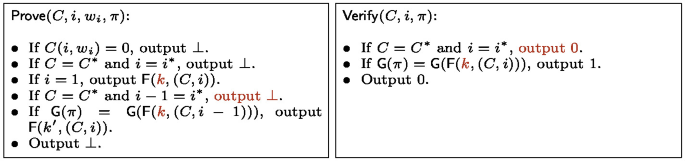
• The proving program takes as input a Boolean circuit $C :\{0,1\}^\lambda \times \{0,1\}^m\rightarrow \{0,1\}$, an instance number $i \in [2^\lambda ]$, a witness $w \in \{0,1\}^m$ for instance i as well as a proof $\pi$ for the first $i - 1$ instances. The program validates the proof on the first $i - 1$ instances and that $C(i, w) = 1$. If both checks pass, then the program outputs a proof for instance i. Otherwise, it outputs $\bot$.

• The verification program takes as input the circuit C, the final instance number $t \in [2^\lambda ]$, and a proof $\pi$. It outputs a bit indicating whether the proof is valid or not. In this case, outputting 1 indicates that $\pi$ is a valid proof on instances $(1, \ldots , t)$.

Construction 3.1

(Batch Argument for Index Languages). Let $\lambda$ be a security parameter and $s = s(\lambda )$ be a bound on the size of the Boolean circuit. We construct a BARG scheme that supports index languages with up to $T = 2^\lambda$ instances (i.e., which suffices to support an arbitrary polynomial number of instances) and circuits of size at most s. The instance indices will be taken from the set $[2^\lambda ]$. For ease of notation, we use the set $[2^\lambda ]$ and the set $\{0,1\}^\lambda$ interchangably in the following description. Our construction relies on the following primitives:

• Let $\textsf{PRF}$ be a puncturable PRF with key space $\{0,1\}^{\lambda }$, domain $\{0,1\}^{s}\times \{0,1\}^{\lambda }$ and range $\{0,1\}^{\lambda }$.

• Let $i\mathcal {O}$ be an indistinguishability obfuscator.

• Let $\textsf{PRG}$ be a pseudorandom generator with domain $\{0,1\}^{\lambda }$ and range $\{0,1\}^{2\lambda }$.

We define our batch argument $\varPi _{\textsf{BARG}}= (\textsf{Gen}, \textsf{P}, \textsf{V})$ for index languages as follows:

• $\textsf{Gen} (1^\lambda , 1^{s})$: On input the security parameter $\lambda$, and a bound on the circuit size $s$, the setup algorithm starts by sampling a PRF key $K \leftarrow \textsf{PRF}.\textsf{Setup} (1^{\lambda })$. The setup algorithm then defines the proving program $\textsf{Prove} [K]$ and the verification program $\textsf{Verify} [K]$ as follows:

  The setup algorithm constructs $\textsf{ObfProve} \leftarrow i\mathcal {O} (1^{\lambda },\textsf{Prove} [K])$ and $\textsf{ObfVerify} \leftarrow i\mathcal {O} (1^{\lambda },\textsf{Verify} [K])$. Note that both the proving circuit $\textsf{Prove} [K]$ and $\textsf{Verify} [K]$ are padded to the maximum size of any circuit that appears in the proof of Theorem 3.3. Finally, it outputs the common reference string $\textsf{crs} = (\textsf{ObfProve}, \textsf{ObfVerify})$.

• $\textsf{P} (\textsf{crs}, C, (w_1, \ldots , w_t))$: On input $\textsf{crs} = (\textsf{ObfProve},\textsf{ObfVerify})$, a Boolean circuit $C :\{0,1\}^\lambda \times \{0,1\}^m\rightarrow \{0,1\}$, and a collection of witnesses $w_1, \ldots , w_t \in \{0,1\}^m$, the prover algorithm does the following:

  • Compute $\pi _1\leftarrow \textsf{ObfProve} (C,1,w_1,\bot )$.

  • For $i = 2, \ldots , t$, compute $\pi _i \leftarrow \textsf{ObfProve} (C, i, w_i, \pi _{i-1})$.

  • Output $\pi _t$.

• $\textsf{V} (\textsf{crs}, C, t, \pi )$: On input $\textsf{crs} = (\textsf{ObfProve},\textsf{ObfVerify})$, a Boolean circuit $C :\{0,1\}^\lambda \times \{0,1\}^m\rightarrow \{0,1\}$, the instance count $t \in [2^\lambda ]$, and a proof $\pi \in \{0,1\}^{\lambda }$, the verification algorithm outputs $\textsf{ObfVerify} (C, t, \pi )$.

Fig. 1.

$\text {Program}~\textsf{Prove} [K]$

Fig. 2.

Program $\textsf{Verify} [K]$

Completeness and security analysis. We now state the completeness and security properties of Construction 3.1, but defer their proofs to the full version of this paper.

Theorem 3.2

(Completeness). If $i\mathcal {O}$ is correct, then Construction 3.1 is complete.

Theorem 3.3

(Soundness). If $\textsf{PRF}$ is functionality preserving and a secure puncturable PRF, $\textsf{PRG}$ is a secure PRG, and $i\mathcal {O}$ is secure, then Construction 3.1 satisfies non-adaptive soundness.

Theorem 3.4

(Succinctness). Construction 3.1 is fully succinct.

Theorem 3.5

(Zero Knowledge). Construction 3.1 satisfies perfect zero knowledge.

4 Non-Adaptive BARGs for $\textsf{NP}$ from BARGs for Index Languages

In this section, we describe an adaptation of the compiler of Choudhuri et al.  [CJJ21b] for upgrading a batch argument for index language to a batch argument for $\textsf{NP}$. The transformation of Choudhuri et al. relied on somewhere extractable commitments, which can be based on standard lattice assumptions [HW15, CJJ21b] or pairing-based assumptions [WW22]. Here, we show that the same transformation is possible using the positional accumulators introduced by Koppula et al.  [KLW15]. The advantage of basing the transformation on positional accumulators is that we can construct positional accumulators directly from indistinguishability obfuscation and one-way functions, so we can apply the transformation to Construction 3.1 from Sect. 3 to obtain a fully succinct batch argument for $\textsf{NP}$ from the same set of assumptions. A drawback of using positional accumulators in place of somewhere extractable commitments is that our transformation can only provide non-adaptive soundness, whereas the Choudhuri et al. transformation satisfies the stronger notion of semi-adaptive somewhere extractability.

Positional accumulators. Like a somewhere statistically binding (SSB) hash function [HW15], a positional accumulator allows a user to compute a short “digest” or “hash” y of a long input $(x_1, \ldots , x_t)$. The scheme supports local openings where the user can open y to the value $x_i$ at any index i with a short opening $\pi _i$. The security property is that the hash value y is statistically binding at a certain (hidden) index $i^*$. An important difference between positional accumulators and somewhere statistically binding hash functions is that positional accumulators are statistically binding for the hash y of a specific tuple of inputs $(x_1, \ldots , x_t)$ while SSB hash functions are binding for all hash values. We give the definition below. Our definition is a simplification of the corresponding definition of Koppula et al.  [KLW15, §4] and we summarize the main differences in Remark 4.3.

Definition 4.1

(Positional Accumulators [KLW15, adapted]). Let $\ell \in {\mathbb N}$ be an input length. A positional accumulator scheme for inputs of length $\ell$ is a tuple of PPT algorithms $\varPi _{\textsf{PA}} = (\textsf{Setup}, \textsf{SetupEnforce}, \textsf{Hash}, \textsf{Open}, \textsf{Verify})$ with the following properties:

• $\textsf{Setup} (1^\lambda , 1^\ell )\rightarrow \textsf{pp}$: On input the security parameter $\lambda$ and the input length $\ell$, the setup algorithm outputs a set of public parameters $\textsf{pp}$.

• $\textsf{SetupEnforce} (1^\lambda ,1^\ell ,(x_1,\ldots ,x_t),i^*)\rightarrow \textsf{pp}$: On input the security parameter $\lambda$, an input length $\ell$, a tuple of inputs $x_1,\ldots ,x_t\in \{0,1\}^\ell$, and an index $i^* \in [t]$, the enforcing setup algorithm outputs a set of public parameters $\textsf{pp}$.

• $\textsf{Hash} (\textsf{pp}, (x_1,\ldots ,x_t)) \rightarrow y$: On input the public parameters $\textsf{pp}$, a tuple of inputs $x_1\in \{0,1\}^\ell ,\ldots ,x_t\in \{0,1\}^\ell$, the hash algorithm outputs a value y. This algorithm is deterministic.

• $\textsf{Open} (\textsf{pp},(x_1,\ldots ,x_t),i)\rightarrow \pi$: On input the public parameters $\textsf{pp}$, a tuple of inputs $x_1\in \{0,1\}^\ell ,\ldots ,x_t\in \{0,1\}^\ell$ and an index $i\in [t]$, the opening algorithm outputs an opening $\pi$.

• $\textsf{Verify} (\textsf{pp},y,x,i,\pi )\rightarrow \{0,1\}$: On input the public parameters $\textsf{pp}$, a hash value y, an input $x\in \{0,1\}^\ell$, an index $i\in \{0,1\}^\lambda$, and an opening $\pi$, the verification algorithm outputs a bit $\{0,1\}$.

Moreover, the positional accumulator $\varPi _{\textsf{PA}}$ should satisfy the following properties:

• Correctness: For all security parameters $\lambda \in {\mathbb N}$ and input lengths $\ell \in \mathbb {N}$, all polynomials $t=t(\lambda )$, indices $i\in [t]$, and inputs $x_1,\ldots ,x_t\in \{0,1\}^\ell$, it holds that

  $$ \Pr \left[ \textsf{Verify} (\textsf{pp},y,x_i,i,\pi ) = 1 : \begin{array}{c} \textsf{pp} \leftarrow \textsf{Setup} (1^\lambda ,1^\ell ), \\ y \leftarrow \textsf{Hash} (\textsf{pp},(x_1,\ldots ,x_t)), \\ \pi \leftarrow \textsf{Open} (\textsf{pp},(x_1,\ldots ,x_t),i) \end{array} \right] = 1. $$

• Succinctness: The length of the hash value y output by $\textsf{Hash}$ and the length of the proof $\pi$ output by $\textsf{Open}$ in the completeness experiment satisfy $|y| = \textsf{poly} (\lambda , \ell )$ and $|\pi | = \textsf{poly} (\lambda , \ell )$.

• Setup indistinguishability: For a security parameter $\lambda$, a bit $b \in \{0,1\}$, and an adversary $\mathcal {A}$, we define the setup-indistinguishability experiment as follows:

  • Algorithm $\mathcal {A}$ starts by choosing inputs $x_1,\ldots ,x_t\in \{0,1\}^\ell$, and an index $i \in [t]$.

  • If $b = 0$, the challenger samples $\textsf{pp} \leftarrow \textsf{Setup} (1^\lambda , 1^\ell )$. Otherwise, if $b = 1$, the challenger samples $\textsf{pp} \leftarrow \textsf{SetupEnforce} (1^\lambda , 1^\ell , (x_1, \ldots , x_t), i)$. It gives $\textsf{pp}$ to $\mathcal {A}$.

  • Algorithm $\mathcal {A}$ outputs a bit $b' \in \{0,1\}$, which is the output of the experiment.

  We say that $\varPi _{\textsf{PA}}$ satisfies $(\tau , \varepsilon )$-setup-indistinguishability if for all adversaries running in time $\tau = \tau (\lambda )$, there exists $\lambda _\mathcal {A}\in {\mathbb N}$ such that for all $\lambda >\lambda _\mathcal {A}$

  $$\begin{aligned} |\Pr [b' = 1 \mid b = 0] - \Pr [b' = 1 \mid b = 1]| \le \varepsilon (\lambda ). \end{aligned}$$

  in the setup-indistinguishability experiment.

• Enforcing: Fix a security parameter $\lambda \in {\mathbb N}$, block size $\ell \in \mathbb {N}$, a polynomial $t=t(\lambda )$, an index $i^* \in [t]$, and a set of inputs $x_1,\ldots ,x_t$. We say that a set of public parameters $\textsf{pp}$ are “enforcing” for a tuple $(x_1, \ldots , x_t, i^*)$ if there does not exist a pair $(x, \pi )$ where $x \ne x_{i^*}$, $\textsf{Verify} (\textsf{pp}, y, x, i^*, \pi ) = 1$, and $y \leftarrow \textsf{Hash} (\textsf{pp}, (x_1, \ldots , x_t))$. We say that the positional accumulator is enforcing if for every polynomial $\ell = \ell (\lambda )$, $t= t(\lambda )$, index $i^* \in [t]$ and inputs $x_1,\ldots ,x_t\in \{0,1\}^\ell$, there exists a negligible function $\textsf{negl} (\cdot )$ such that for all $\lambda \in {\mathbb N}$,

  $$\begin{aligned}{} & {} \Pr [\textsf{pp} \text { is ``enforcing'' for }(x_1,\ldots ,x_T, i^*) : \\{} & {} \qquad \qquad \qquad \textsf{pp} \leftarrow \textsf{SetupEnforce} (1^\lambda ,1^\ell ,(x_1,\ldots ,x_t),i^*)] \ge 1 -\textsf{negl} (\lambda ), \end{aligned}$$

  where the probability is taken over the random coins of $\textsf{SetupEnforce}$.

Theorem 4.2

(Positional Accumulators [KLW15]). Assuming the existence of an indistinguishability obfuscation scheme and one-way functions, there exists a positional accumulator for arbitrary polynomial input lengths $\ell = \ell (\lambda )$.

Remark 4.3

(Comparison with [KLW15]). Definition 4.1 describes a simplified variant of the positional accumulator from Koppula et al.  [KLW15, §4]. Specifically, we instantiate their construction with an (implicit) bound of $T = 2^\lambda$ for the number of values that can be accumulated. The positional accumulators from Koppula et al. also supports insertions (i.e., “writes”) to the accumulator structure, whereas in our setting, all of the inputs are provided upfront (as an input to $\textsf{Hash}$).

Construction 4.4

(Batch Argument for $\textsf{NP}$ Languages). Let $\lambda$ be a security parameter and $s = s(\lambda )$ be a bound on the size of the Boolean circuit. We construct a BARG scheme that supports arbitrary $\textsf{NP}$ languages with up to $T = 2^\lambda$ instances (i.e., which suffices to support an arbitrary polynomial number of instances) and Boolean circuits of size at most s. For ease of notation, we use the set $[2^\lambda ]$ and the set $\{0,1\}^\lambda$ interchangably in the following description. Our construction relies on the following primitives:

• Let $\varPi _{\textsf{PA}} = (\textsf{PA}.\textsf{Setup}, \textsf{PA}.\textsf{SetupEnforce}, \textsf{PA}.\textsf{Hash}, \textsf{PA}.\textsf{Open}, \textsf{PA}.\textsf{Verify})$ be a positional accumulator for inputs of length $\ell$.

• Let $\varPi _\mathsf {Index\textsf{BARG}}=(\mathsf {Index\textsf{BARG}}.\textsf{Gen},\mathsf {Index\textsf{BARG}}.\textsf{P},\mathsf {Index\textsf{BARG}}.\textsf{V})$ be a BARG for index languages (that supports up to $T = 2^\lambda$ instances).⁵

We define our batch argument $\varPi _{\textsf{BARG}}= (\textsf{Gen}, \textsf{P}, \textsf{V})$ for batch circuit satisfiability languages as follows:

• $\textsf{Gen} (1^\lambda ,1^\ell ,1^{s})$: On input the security parameter $\lambda$, the statement length $\ell$, and a bound on the circuit size s, sample $\textsf{pp} \leftarrow \textsf{PA}.\textsf{Setup} (1^\lambda ,1^\ell )$. Let $s'$ be a bound on the size of the following circuit:

  Then, sample $\mathsf {Index\textsf{BARG}}.\textsf{crs} \leftarrow \mathsf {Index\textsf{BARG}}.\textsf{Gen} (1^\lambda ,1^{s'})$. Output the common reference string $\textsf{crs} = (\textsf{pp},\mathsf {Index\textsf{BARG}}.\textsf{crs})$.

• $\textsf{P} (\textsf{crs},C,(x_1,\ldots ,x_t),(w_1,\ldots ,w_t))$: On input the common reference string $\textsf{crs} = (\textsf{pp},\mathsf {Index\textsf{BARG}}.\textsf{crs})$, a Boolean circuit $C :\{0,1\}^\ell \times \{0,1\}^m \rightarrow \{0,1\}$, statements $x_1, \ldots , x_t\in \{0,1\}^\ell$, and witnesses $w_1, \ldots , w_t\in \{0,1\}^m$, compute $h\leftarrow \textsf{PA}.\textsf{Hash} (\textsf{pp},(x_1,\ldots ,x_t))$. Then, for each $i\in [t]$, let $\sigma _i\leftarrow \textsf{PA}.\textsf{Open} (\textsf{pp},(x_1,\ldots ,x_t),i)$ and let $w'_i = (x_i,\sigma _i,w_i)$. Output $\pi \leftarrow \mathsf {Index\textsf{BARG}}.\textsf{P} (\mathsf {Index\textsf{BARG}}.\textsf{crs},C'[\textsf{pp}, h, C],t,(w'_1,\ldots ,w'_t))$, where $C'[\textsf{pp},h,C]$ is the circuit for the index relation from Fig. 3.

• $\textsf{V} (\textsf{crs},C,(x_1,\ldots ,x_t),\pi )$: On input the common reference string $\textsf{crs} = (\textsf{pp},\mathsf {Index\textsf{BARG}}.\textsf{crs})$, the Boolean circuit $C :\{0,1\}^\ell \times \{0,1\}^m \rightarrow \{0,1\}$, instances $x_1, \ldots , x_t\in \{0,1\}^\ell$, and a proof $\pi$, the verification algorithm computes $h\leftarrow \textsf{PA}.\textsf{Hash} (\textsf{pp},(x_1,\ldots ,x_t))$ and outputs $\mathsf {Index\textsf{BARG}}.\textsf{V} (\mathsf {Index\textsf{BARG}}.\textsf{crs},C'[\textsf{pp}, h, C],t,\pi )$, where $C'[\textsf{pp},h,C]$ is the circuit for the index relation from Fig. 3.

Fig. 3.

The Boolean circuit $C'[\textsf{pp}, h, C]$ for an index relation

Completeness and security analysis. We now state the completeness and security properties of Construction 4.4, but defer their formal analysis to the full version of this paper.

Theorem 4.5

(Completeness). If $\varPi _\mathsf {Index\textsf{BARG}}$ is complete and $\varPi _\textsf{PA}$ is correct, then Construction 4.4 is complete.

Theorem 4.6

(Soundness). Suppose $\varPi _\mathsf {Index\textsf{BARG}}$ satisfies non-adaptive soundness, $\varPi _\textsf{PA}$ satisfies setup-indistinguishability and is enforcing. Then, Construction 4.4 satisfies non-adaptive soundness.

Theorem 4.7

(Succinctness). If $\varPi _\mathsf {Index\textsf{BARG}}$ is succinct (resp., fully succinct), $\varPi _\textsf{PA}$ is efficient, then Construction 4.4 is succinct (resp., fully succinct).

Theorem 4.8

(Zero Knowledge). If $\varPi _\mathsf {Index\textsf{BARG}}$ is perfect zero-knowledge, then Construction 4.4 is perfect zero-knowledge.

Remark 4.9

(Weaker Notions of Zero Knowledge). If $\varPi _\mathsf {Index\textsf{BARG}}$ satisfies computational (resp., statistical) zero-knowledge, then Construction 4.4 satisfies computational (resp., statistical) zero-knowledge. In other words, Construction 4.4 preserves the zero-knowledge property on the underlying index BARG.

5 Updatable Batch Argument for $\textsf{NP}$

We say that a BARG scheme is updatable if it supports an a priori unbounded number of statements (see Definition 2.7) and the prover algorithm is updatable. Formally, we replace the prover algorithm $\textsf{P}$ in the BARG with an $\textsf{UpdateP}$ algorithm. The $\textsf{UpdateP}$ algorithm takes in statements $(x_1,\ldots ,x_t)$, a proof $\pi _t$ on these t statements, a new statement $x_{t+1}$, along with an associated witness $w_{t+1}$, and outputs an “updated” proof $\pi _{t + 1}$ on the new set of statements $(x_1, \ldots , x_{t + 1})$. The updated proof should continue to satisfy the same succinctness requirements as before. We give the formal definition below:

Definition 5.1

(Updatable BARGs). An updatable batch argument (BARG) for the language of Boolean circuit satisfiability consists of a tuple of PPT algorithms $\varPi _{\textsf{BARG}} = (\textsf{Gen},\textsf{UpdateP},\textsf{V})$ with the following properties:

• $\textsf{Gen} (1^\lambda ,1^\ell ,1^{s}) \rightarrow \textsf{crs}$: On input the security parameter $\lambda \in {\mathbb N}$, a bound on the instance size $\ell \in {\mathbb N}$, and a bound on the maximum circuit size $s\in {\mathbb N}$, the generator algorithm outputs a common reference string $\textsf{crs}$.

• $\textsf{UpdateP} (\textsf{crs}, C, (x_1,\ldots ,x_t), \pi _t, x_{t+1}, w_{t+1}) \rightarrow \pi _{t + 1}$: On input the common reference string $\textsf{crs}$, a Boolean circuit $C :\{0,1\}^\ell \times \{0,1\}^m\rightarrow \{0,1\}$, a list of statements $x_1,\ldots ,x_t\in \{0,1\}^\ell$, a proof $\pi _t$, a new statement $x_{t+1}\in \{0,1\}^\ell$ and witness $w_{t+1}\in \{0,1\}^m$, the update algorithm outputs an updated proof $\pi _{t+1}$. Note that the list of statements $(x_1, \ldots , x_t)$ is allowed to be empty. We will write $\bot$ to denote an empty list of statements.

• $\textsf{V} (\textsf{crs},C,(x_1,\ldots ,x_t),\pi ) \rightarrow b$: On input the common reference string $\textsf{crs}$, a Boolean circuit $C :\{0,1\}^\ell \times \{0,1\}^m\rightarrow \{0,1\}$, a list of statements $x_1,\ldots ,x_t\in \{0,1\}^\ell$, and a proof $\pi$, the verification algorithm outputs a bit $b\in \{0,1\}$.

An updatable BARG scheme should satisfy the following properties:

• Completeness: For every security parameter $\lambda \in {\mathbb N}$ and bounds $t \in {\mathbb N}$, $\ell \in {\mathbb N}$, and $s\in {\mathbb N}$, Boolean circuits $C :\{0,1\}^\ell \times \{0,1\}^m\rightarrow \{0,1\}$ of size at most $s$, any collection of statements $x_1,\ldots ,x_t\in \{0,1\}^\ell$ and associated witnesses $w_1, \ldots , w_t \in \{0,1\}^m$ where $C(x_i, w_i) = 1$ for all $i \in [t]$, we have that

  $$\Pr \begin{array}{c}\begin{array}{l} \forall i \in [t]: \textsf{V} (\textsf{crs},C,(x_1,\ldots ,x_i),\pi _{i})=1\end{array}:\begin{array}{c}\textsf{crs} \leftarrow \textsf{Gen} (1^\lambda ,1^\ell ,1^s)\,, \pi _0 \leftarrow \bot , \\ \pi _i\leftarrow \textsf{UpdateP} (\textsf{crs},C,(x_1,\ldots ,x_{i-1}),\pi _{i-1},x_i,w_i) \\ \qquad \qquad \text {for all }i \in [t] \end{array}\end{array}=1. $$

• Succinctness: Similar to Definition 2.6, we require two succinctness properties:

  • Succinct proof size: There exists a universal polynomial $\textsf{poly} (\cdot , \cdot , \cdot )$, such that for every $i \in [t]$, $|\pi _{i}| = \textsf{poly} (\lambda , \log i, s)$ in the completeness experiment above.

  • Succinct verification time: There exists a universal polynomial $\textsf{poly} (\cdot , \cdot , \cdot )$ such that for all $i \in [t]$, the verification algorithm $\textsf{V} (\textsf{crs},C,(x_1,\ldots ,x_i),\pi _i)$ runs in time $\textsf{poly} (\lambda , i, \ell ) + \textsf{poly} (\lambda , \log i, s)$ in the completeness experiment above.

• Soundness: The soundness definition is defined exactly as in Definition 2.6.

• Perfect zero knowledge: The zero-knowledge definition is defined exactly as in Definition 2.6.

5.1 Updatable BARGs for $\textsf{NP}$ from Indistinguishability Obfuscation

We now give a direct construction of an updatable batch argument for NP languages from indistinguishability obfuscation together with somewhere statistically binding (SSB) hash functions [HW15]. We start with a construction that provides non-adaptive soundness. We then show to use complexity leveraging to obtain a construction with adaptive soundness.

Two-to-one somewhere statistically binding hash functions. Our construction will rely on a two-to-one somewhere statistically binding (SSB) hash function [OPWW15]. Informally, a two-to-one SSB hash function hashes two input blocks to an output whose size is comparable to the size of a single block. We recall the definition below:

Definition 5.2

(Two-to-One Somewhere Statistically Binding Hash Function [OPWW15]). Let $\lambda$ be a security parameter. A two-to-one somewhere statistically binding (SSB) hash function with block size $\ell _{\textsf{blk}}= \ell _{\textsf{blk}}(\lambda )$ and output size $\ell _{\textsf{out}}= \ell _{\textsf{out}}(\lambda , \ell _{\textsf{blk}})$ is a tuple of efficient algorithms $\varPi _{\textsf{SSB}}= (\textsf{Gen}, \textsf{GenTD}, \textsf{LocalHash})$ with the following properties:

• $\textsf{Gen} (1^\lambda , 1^{\ell _{\textsf{blk}}})\rightarrow \textsf{hk}$: On input the security parameter $\lambda$ and the block size $\ell _{\textsf{blk}}$, the generator algorithm outputs a hash key $\textsf{hk}$.

• $\textsf{GenTD} (1^\lambda ,1^{\ell _{\textsf{blk}}},i^*)\rightarrow \textsf{hk}$: On input a security parameter $\lambda$, a block size $\ell _{\textsf{blk}}$, and an index $i^* \in \{0,1\}$, the trapdoor generator algorithm outputs a hash key $\textsf{hk}$.

• $\textsf{LocalHash} (\textsf{hk},x_0,x_1)\rightarrow y$: On input a hash key $\textsf{hk}$ and two inputs $x_0, x_1 \in \{0,1\}^{\ell _{\textsf{blk}}}$, the hash algorithm outputs a hash $y\in \{0,1\}^{\ell _{\textsf{out}}}$.

Moreover, $\varPi _{\textsf{SSB}}$ should satisfy the following requirements:

• Succinctness: The output length $\ell _{\textsf{out}}$ satisfies $\ell _{\textsf{out}}(\lambda , \ell _{\textsf{blk}}) = \ell _{\textsf{blk}}\cdot (1+1/\varOmega (\lambda )) + \textsf{poly} (\lambda )$.

• Index hiding: For a security parameter $\lambda$, a bit $b \in \{0,1\}$, and an adversary $\mathcal {A}$, we define the index-hiding experiment as follows:

  • Algorithm $\mathcal {A}$ starts by choosing a block size $\ell _{\textsf{blk}}$, and an index $i \in \{0,1\}$.

  • If $b = 0$, the challenger samples $\textsf{hk} _0 \leftarrow \textsf{Gen} (1^\lambda , 1^{\ell _{\textsf{blk}}})$. Otherwise, if $b = 1$, the challenger samples $\textsf{hk} _1 \leftarrow \textsf{GenTD} (1^\lambda , 1^{\ell _{\textsf{blk}}}, i)$. It gives $\textsf{hk} _b$ to $\mathcal {A}$.

  • Algorithm $\mathcal {A}$ outputs a bit $b' \in \{0,1\}$, which is the output of the experiment.

  We say that $\varPi _{\textsf{SSB}}$ satisfies $(\tau , \varepsilon )$-index-hiding, if for all adversaries running in time $\tau = \tau (\lambda )$, there exists $\lambda _\mathcal {A}\in {\mathbb N}$ such that for all $\lambda >\lambda _\mathcal {A}$, $|\Pr [b' = 1 \mid b = 0] - \Pr [b' = 1 \mid b = 1]| \le \varepsilon (\lambda )$ in the index-hiding experiment.

• Somewhere statistically binding: Let $\lambda \in {\mathbb N}$ be a security parameter and $\ell \in {\mathbb N}$ be an input length. We say a hash key $\textsf{hk}$ is"statistically binding" at index $i \in \{ 0,1 \}$, if there does not exist two inputs $(x_0,x_1)$ and $(x^* _0,x^* _1)$ such that $x^* _{i}\ne x_{i}$ and $\textsf{Hash} (\textsf{hk},(x_0,x_1)) = \textsf{Hash} (\textsf{hk},(x^* _0,x^* _1))$. We then say that the hash function is somewhere statistically binding if for all polynomials $\ell _{\textsf{blk}}= \ell _{\textsf{blk}}(\lambda )$, there exists a negligible function $\textsf{negl} (\cdot )$ such that for all indices $i^*\in \{0,1\}$ and all $\lambda \in {\mathbb N}$,

  $$\begin{aligned} \Pr [\textsf{hk} \text { is statistically binding at index }i : \textsf{hk} \leftarrow \textsf{GenTD} (1^\lambda ,1^{\ell _{\textsf{blk}}},i)] \ge 1 -\textsf{negl} (\lambda ). \end{aligned}$$

Theorem 5.3

(Somewhere Statistically-Binding Hash Functions [OPWW15]). Under standard number-theoretic assumptions (e.g., DDH, DCR, LWE, or $\phi$-Hiding), there exists a two-to-one somewhere statistically binding hash function for arbitrary polynomial block size $\ell _{\textsf{blk}}=\ell _{\textsf{blk}}(\lambda )$.

Notation. Our updatable BARG construction uses a tree-based construction. Before describing the construction, we introduce some notation. First, for an integer $t < 2^{d}$, we write $\textsf{bin}_d(t)\in \{0,1\}^{d}$ to denote the d-bit binary representation of t. For two strings $\textsf{ind} \in \{0,1\}^*$, $\textsf{ind} '\in \{0,1\}^*$, let $\textsf{pad}(\textsf{ind})$ and $\textsf{pad}(\textsf{ind} ')$ be the respective strings padded with zeros to the length $\max \{|\textsf{ind} |,|\textsf{ind} '|\}$. We say $\textsf{ind} \le \textsf{ind} '$ if $\textsf{pad}(\textsf{ind})$ comes before $\textsf{pad}(\textsf{ind} ')$ lexicographically. For strings $s_1, s_2 \in \{0,1\}^*$, we write $s_1 \Vert s_2$ to denote their concatenation. We say that a string $x\in \{0,1\}^*$ is a prefix of a string $y\in \{0,1\}^*$ if there exists a string $z\in \{0,1\}^*$ such that $y=x\Vert z$.

Binary trees. A binary tree $\varGamma$ of height d consists of nodes where each node is indexed by a binary string of length at most d. We now define a recursive labeling scheme for the nodes of the tree; subsequently, we will refer to nodes by their labels.

• Root node: The root node is labeled with the empty string $\varepsilon$.

• Child nodes: The left child of node $\textsf{ind}$ has label $\textsf{ind} \Vert 0$ and the right child has label $\textsf{ind} \Vert 1$. We also say that node $\textsf{ind} \Vert 0$ is the “left sibling” of the node $\textsf{ind} \Vert 1$.

We define the level of a node $\textsf{ind}$ by $\textsf{level}(\textsf{ind})= d-|\textsf{ind} |$. In particular, the root node is at level d while the leaf nodes are at level 0. We write $\{0,1\}^{\le d}$ to denote the set of node labels associated in the binary tree (i.e., the set of all binary strings of length at most d). Finally, we can also associate each node in the binary tree with a value; formally, for a binary tree $\varGamma$ we write $\textsf{val}(\textsf{ind})$ to denote the value associated with the node $\textsf{ind}$. When we write $(\varGamma , \textsf{val}(\cdot ))$, we imply our binary tree has been initialized with the corresponding value function. Finally, we define the notion of a “path” and a “frontier” of a node in a binary tree $\varGamma$:

• Path of a node: We define the path associated with a node $\textsf{ind} \in \{0,1\}^{\le d}$ as

  $$\begin{aligned} \textsf{path}(\textsf{ind})=\{ \textsf{ind} ' \mid \textsf{ind} '\in \{0,1\}^{\le d}\text { and }\textsf{ind} '\text { is a prefix of }\textsf{ind} \}. \end{aligned}$$

  Namely, $\textsf{path}(\textsf{ind})$ consists of the nodes along the path from the root to $\textsf{ind}$.

• Frontier of a node: For any $\textsf{ind} \in \{0,1\}^{\le d}$, we define

  $$ \textsf{frontier}(\textsf{ind}) = \{ \textsf{ind} \} \cup \{ \textsf{ind} ' \in \{0,1\}^{\le d} \mid \textsf{ind} '\text { is a left sibling of a node in }\textsf{path}(\textsf{ind}) \}. $$

Construction 5.4

(Non-Adaptive Updatable Batch Argument for $\textsf{NP}$ ). Let $\lambda$ be a security parameter, $\ell = \ell (\lambda )$ be the statement size, and $s = s(\lambda )$ be a bound on the size of the Boolean circuit. We construct an updatable BARG scheme that supports $\textsf{NP}$ languages with up to $T = 2^\lambda$ instances of length $\ell$ and circuit size at most s. Note that setting $T = 2^\lambda$ means the construction support an arbitrary polynomial number of instances. Our construction relies on the following primitives:

• Let $\varPi _\textsf{SSB} =(\textsf{SSB}.\textsf{Gen},\textsf{SSB}.\textsf{GenTD},\textsf{SSB}.\textsf{LocalHash})$ be a two-to-one somewhere statistically binding hash function with output length $\ell _{\textsf{out}}= \ell _{\textsf{out}}(\lambda , \ell _{\textsf{blk}})$, where $\ell _{\textsf{blk}}$ denotes the block length. Our construction will consider a binary tree of depth $d = \lambda$, and we define a sequence of block lengths $\ell _{0}, \ldots , \ell _{d}$ where $\ell _{0}=\ell$ and for $j \in [d]$, let $\ell _{j} = \ell _{\textsf{out}}(\lambda , \ell _{j - 1})$.⁶ Let $\ell _{\max } = \max (\ell _{0}, \ldots , \ell _{j})$.

• Let $\varPi _\textsf{PRF} =(\textsf{PRF}.\textsf{Setup},\mathsf {PRF.Puncture},\mathsf {PRF.Eval})$ be a puncturable PRF with key space $\{0,1\}^{\lambda }$, domain $\{0,1\}^{\le s} \times \{0,1\}^{\le \ell _{\max }}\times \{0,1\}^{d}$ and range $\{0,1\}^{\lambda }$.

• Let $i\mathcal {O}$ be an indistinguishability obfuscator for general circuits.

• Let $\textsf{PRG}$ be a pseudorandom generator with domain $\{0,1\}^{\lambda }$ and range $\{0,1\}^{2\lambda }$.

We define our updatable batch argument $\varPi _{\textsf{BARG}}= (\textsf{Gen}, \textsf{UpdateP}, \textsf{Verify})$ for $\textsf{NP}$ languages as follows:

Fig. 4.

$\text {Program}~\textsf{Prove} [K,\textsf{hk} ]$

Fig. 5.

$\text {Program}~\textsf{Verify} [K]$

• $\textsf{Gen} (1^\lambda , 1^\ell , 1^{s})$: On input the security parameter $\lambda$, the statement size $\ell$, and a bound on the circuit size $s$, the setup algorithm starts by sampling a PRF key $K \leftarrow \textsf{PRF}.\textsf{Setup} (1^{\lambda })$. For $j\in [d]$, sample $\textsf{hk} _j\leftarrow \textsf{SSB}.\textsf{Gen} (1^\lambda ,1^{{\ell _{j-1}}})$, Let $\textsf{hk} \leftarrow (\textsf{hk} _1,\ldots ,\textsf{hk} _d)$ and define the proving program $\textsf{Prove} [K,\textsf{hk} ]$ and the verification program $\textsf{Verify} [K]$ as follows:

  The setup algorithm obfuscates the above programs to obtain $\textsf{ObfProve} \leftarrow i\mathcal {O} (1^{\lambda },\textsf{Prove} [K,\textsf{hk} ])$ and $\textsf{ObfVerify} \leftarrow i\mathcal {O} (1^{\lambda },\textsf{Verify} [K])$. Note that both the proving circuit $\textsf{Prove} [K,\textsf{hk} ]$ and $\textsf{Verify} [K]$ are padded to the maximum size of any circuit that appears in the proof of Theorem 5.6. Finally, it outputs the common reference string $\textsf{crs} = (\textsf{ObfProve}, \textsf{ObfVerify},\textsf{hk})$.

• $\textsf{UpdateP} (\textsf{crs},C,(x_1,\ldots ,x_t),\pi _t,x_{t+1},w_{t+1})$: On input a common reference string $\textsf{crs} = (\textsf{ObfProve},\textsf{ObfVerify},\textsf{hk})$, a Boolean circuit $C :\{0,1\}^{\ell } \times \{0,1\}^m\rightarrow \{0,1\}$, a set of statements $x_1,\ldots ,x_t,x_{t+1} \in \{0,1\}^{\ell }$, a proof $\pi _t = \{(\textsf{ind},\pi _\textsf{ind})\}_{\textsf{ind} \in \mathcal {I}}$ on the first t statements where $\mathcal {I}\subset \{0,1\}^{\le d}$, and a witness $w_{t+1} \in \{0,1\}^m$, the update algorithm proceeds as follows:

  • 1. If $t=0$, let $\textsf{ind} ^{(1)} = \textsf{bin}_d(0) = 0^d$. Let $\pi \leftarrow \textsf{ObfProve} (C, x_{1}, \bot , \textsf{ind} ^{(1)}, w_{1}, \bot )$ and output $\{(\textsf{ind} ^{(1)}, \pi )\}$.

  • 2. Otherwise, if $t\ne 0$, the update algorithm computes $\textsf{ind} ^{(t)} = \textsf{bin}_d(t-1)$ and checks that $\textsf{frontier}(\textsf{ind} ^{(t)}) = \mathcal {I}$. If the check fails, then the update algorithm outputs $\bot$.

  • 3. Next, the update algorithm constructs a binary tree $({\varGamma _{\textsf{hash}}},\textsf{val}_{\textsf{hash}}) \leftarrow \textsf{Hash} [\textsf{hk} ](x_1, \ldots , x_t)$ of depth d whose values correspond to the statements $(x_1, \ldots , x_t)$ and their hashes. Specifically, we define the $\textsf{Hash} [\textsf{hk} ]$ function as follows:

    Essentially, $\textsf{Hash} [\textsf{hk} ]$ computes a Merkle tree on the statements $(x_1, \ldots , x_t)$.

  • 4. The update algorithm then defines a binary tree ${\varGamma _{\textsf{proof}}}$ of depth d with the following value function $\textsf{val}_{\textsf{proof}}$:

    • For each index $\textsf{ind} \in \mathcal {I}$, let $\textsf{val}_{\textsf{proof}}(\textsf{ind}) = \pi _{\textsf{ind}}$.

    • Let $\textsf{ind} ^{(t+1)} = \textsf{bin}_d(t)$. Let $\textsf{val}_{\textsf{proof}}(\textsf{ind} ^{(t+1)}) = \textsf{ObfProve} (C,x_{t+1},\bot ,\textsf{ind} ^{(t+1)},w_{t+1},\bot )$.

    • For all other nodes $\textsf{ind} \notin \mathcal {I}$, let $\textsf{val}_{\textsf{proof}}(\textsf{ind}) = \bot$.

    The invariant will be that the nodes $\textsf{ind}$ associated with the frontier of leaf node $t$ (with index $\textsf{bin}_d(t - 1)$) are associated with a proof $\pi _\textsf{ind}$.

  • 5. Let $\textsf{ind} '$ be the longest common prefix to $\textsf{ind} ^{(t)}$ and $\textsf{ind} ^{(t+1)}$. Write $\textsf{ind} ^{(t)} = b_1\cdots b_d$ and $\textsf{ind} '=b_1\cdots b_\rho$, where $\rho = |\textsf{ind} '|$ denotes the length of the common prefix. If $\rho <d-1$, then we apply the following procedure for $k=d-1, \ldots , \rho +1$ to merge proofs:

    • Let $\textsf{ind} = b_1\cdots b_{K}$ and compute

      $$\begin{aligned} \textsf{val}_{\textsf{proof}}(\textsf{ind})\leftarrow \textsf{ObfProve} \left( C,h_1, h_2, \textsf{ind},\textsf{val}_{\textsf{proof}}(\textsf{ind} \Vert 0),\textsf{val}_{\textsf{proof}}(\textsf{ind} \Vert 1) \right) , \end{aligned}$$

      where $h_1 \leftarrow \textsf{val}_{\textsf{hash}}(\textsf{ind} \Vert 0)$ and $h_2 \leftarrow \textsf{val}_{\textsf{hash}}(\textsf{ind} \Vert 1)$.

  • 6. Output the updated proof, $\pi _{t+1}=\{ (\textsf{ind},\textsf{val}_{\textsf{proof}}(\textsf{ind})) \}_{\textsf{ind} \in \textsf{frontier}(\textsf{ind} ^{(t+1)})}$.

• $\textsf{V} (\textsf{crs}, C, (x_1,\ldots ,x_t), \pi )$: On input $\textsf{crs} = (\textsf{ObfProve},\textsf{ObfVerify},\textsf{hk})$, a Boolean circuit $C :\{0,1\}^\ell \times \{0,1\}^m\rightarrow \{0,1\}$, statements $x_1,\ldots ,x_t\in \{0,1\}^\ell$ and a proof $\pi =\{(\textsf{ind},\pi _\textsf{ind})\}_{\textsf{ind} \in \mathcal {I}}$ , the verification algorithm proceeds as follows:

  • 1. The algorithm constructs a binary tree $({\varGamma _{\textsf{hash}}},\textsf{val}_{\textsf{hash}}) \leftarrow \textsf{Hash} [\textsf{hk} ](x_1, \ldots , x_t)$ (defined in Fig. 6) of depth d whose values correspond to the statements $(x_1, \ldots , x_t)$ and their hashes.

  • 2. Let $\textsf{ind} ^{(t)} = \textsf{bin}_d(t-1)$. If $\mathcal {I}\ne \textsf{frontier}(\textsf{ind} ^{(t)})$, output $\bot$.

  • 3. Finally, the verification algorithm checks that $\textsf{ObfVerify} (C,\textsf{val}_{\textsf{hash}}(\textsf{ind}),\textsf{ind},\pi _\textsf{ind})=1$ for all $\textsf{ind} \in \textsf{frontier}(\textsf{ind} ^{(t)})$. If any checks fail, output 0. Otherwise output 1.

Fig. 6.

The function $\textsf{Hash} [\textsf{hk} ](x_1, \ldots , x_t)$

Completeness and security analysis. We now state the completeness and security properties of Construction 5.4, but defer their proofs to the full version of this paper.

Theorem 5.5

(Completeness). If $i\mathcal {O}$ is correct, then Construction 5.4 is complete.

Theorem 5.6

(Soundness). If $\varPi _\textsf{PRF}$ is correct and a secure puncturable PRF, $\textsf{PRG}$ is a secure PRG, $\varPi _\textsf{SSB}$ is a secure statistically binding two-to-one SSB hash and $i\mathcal {O}$ is secure, then Construction 5.4 satisfies non-adaptive soundness.

Theorem 5.7

(Succinctness). If $\varPi _\textsf{SSB}$ is succinct, then, Construction 5.4 is fully succinct.

Theorem 5.8

(Zero-knowledge). Construction 5.4 satisfies perfect zero-knowledge.

Combining Theorems 5.5 to 5.8, we obtain the following corollary:

Corollary 5.9

(Non-Adaptive Updatable BARGs). Assuming the existence of a secure indistinguishability obfuscation scheme and of somewhere extractable hash functions, there exists an updatable batch argument for $\textsf{NP}$.

References

Albrecht, M.R., Cini, V., Lai, R.W.F., Malavolta, G., Thyagarajan, S.: Lattice-based SNARKs: publicly verifiable, preprocessing, and recursively composable. In: CRYPTO (2022)
Asharov, G., Segev, G.: Limits on the power of indistinguishability obfuscation and functional encryption. In: FOCS, pp. 191–209 (2015)
Eli, B.-S., Bentov, I., Horesh, Y., Riabzev, M.: Scalable, transparent, and post-quantum secure computational integrity. IACR Cryptol. ePrint Arch. (2018)
Bitansky, N., et al.: The Hunting of the SNARK. J. Cryptology 30(4), 989–1066 (2016). https://doi.org/10.1007/s00145-016-9241-9
Bitansky, N., Canetti, R., Chiesa, A., Tromer, E.: From extractable collision resistance to succinct non-interactive arguments of knowledge, and back again. In: ITCS (2012)
Bitansky, N., Canetti, R., Chiesa, A., Tromer, E.: Recursive composition and bootstrapping for SNARKS and proof-carrying data. In: STOC, pp. 111–120 (2013)
Bitansky, N., Canetti, R., Ishai, Y., Ostrovsky, R., Paneth, O.: Succinct non-interactive arguments via linear interactive proofs. In: TCC (2013)
Bitansky, N., Canetti, R., Paneth, O., Rosen, A.: On the existence of extractable one-way functions. In: STOC (2014)
Barak, B., et al.: On the (im)possibility of obfuscating programs. In: CRYPTO, pp. 1–18 (2001)
Boyle, E., Goldwasser, S., Ivan, I.: Functional signatures and pseudorandom functions. In: PKC, pp. 501–519 (2014)
Boneh, D., Ishai, Y., Sahai, A., Wu, D.J.: Lattice-based SNARGs and their application to more efficient obfuscation. In: EUROCRYPT (2017)
Boneh, D., Ishai, Y., Sahai, A., Wu, D.J.: Quasi-optimal snargs via linear multi-prover interactive proofs. In: EUROCRYPT, pp. 222–255 (2018)
Boneh, D., Waters, B.: Constrained pseudorandom functions and their applications. In: ASIACRYPT, pp. 280–300 (2013)
Chiesa, A., Hu, Y., Maller, M., Mishra, P., Vesely, N., Ward, N.P.: Marlin: Preprocessing zkSNARKs with universal and updatable SRS. In: EUROCRYPT (2020)
Choudhuri, A.R., Jain, A., Jin, Z.: Non-interactive batch arguments for NP from standard assumptions. In: CRYPTO, pp. 394–423 (2021)
Choudhuri, A.R., Jain, A., Jin, Z.: Snargs for \(\cal{P}\) from LWE. In: FOCS, pp. 68–79 (2021)
Chiesa, A., Ojha, D., Spooner, N.: Post-quantum and transparent recursive proofs from holography. In: EUROCRYPT, Fractal (2020)
Damgård, I., Faust, S., Hazay, C.: Secure two-party computation with low communication. In: TCC (2012)
Devadas, L., Goyal, R., Kalai, Y., Vaikuntanathan, V.: Rate-1 non-interactive arguments for batch-NP and applications. IACR Cryptol. ePrint Arch. (2022)
Gennaro, R., Gentry, C., Parno, B., Raykova, M.: Quadratic span programs and succinct NIZKs without PCPs. In: EUROCRYPT (2013)
Groth, J.: Short pairing-based non-interactive zero-knowledge arguments. In: ASIACRYPT (2010)
Groth, J.: On the size of pairing-based non-interactive arguments. In: EUROCRYPT (2016)
Gentry, C., Wichs, D.: Separating succinct non-interactive arguments from all falsifiable assumptions. In: STOC, pp. 99–108 (2011)
Hubácek, P., Wichs, D.: On the communication complexity of secure function evaluation with long output. In: ITCS, pp. 163–172 (2015)
Jain, A., Lin, H., Sahai, A.: Indistinguishability obfuscation from well-founded assumptions. In: STOC, pp. 60–73 (2021)
Jain, A., Lin, H., Sahai, A.: Indistinguishability obfuscation from LPN over f_p, dlin, and prgs in nc\({\hat{\,}}\)0. In: EUROCRYPT (2022)
Koppula, V., Lewko, A.B., Waters, B.: Indistinguishability obfuscation for turing machines with unbounded memory. In: STOC, pp. 419–428 (2015)
Kiayias, A., Papadopoulos, S., Triandopoulos, S., Zacharias, T.: Delegatable pseudorandom functions and applications. In: ACM CCS, pp. 669–684 (2013)
Lipmaa, H.: Succinct non-interactive zero knowledge arguments from span programs and linear error-correcting codes. In: ASIACRYPT (2013)
Merkle, R.C.: A digital signature based on a conventional encryption function. In: CRYPTO, pp. 369–378 (1987)
Micali, S.: Computationally-sound proofs. In: Proceedings of the Annual European Summer Meeting of the Association of Symbolic Logic (1995)
Naor, M.: On cryptographic assumptions and challenges. In: CRYPTO (2003)
Okamoto, T., Pietrzak, K., Waters, B., Wichs, D.: New realizations of somewhere statistically binding hashing and positional accumulators. In: ASIACRYPT, pp. 121–145 (2015)
Parno, B., Howell, J., Gentry, C., Raykova, M.: Nearly practical verifiable computation. In: IEEE Symposium on Security and Privacy, Pinocchio (2013)
Setty, S.T.V.: Spartan: efficient and general-purpose zkSNARKs without trusted setup. In: CRYPTO (2020)
Sahai, A., Waters, B.: How to use indistinguishability obfuscation: deniable encryption, and more. In: STOC (2014)
Waters, B., Wu, D.J.: Batch arguments for NP and more from standard bilinear group assumptions. In: CRYPTO (2022)
Acknowledgments
We thank the anonymous TCC reviewers for helpful feedback on this work. B. Waters is supported by NSF CNS-1908611, a Simons Investigator award, and the Packard Foundation Fellowship. D. J. Wu is supported by NSF CNS-2151131, CNS-2140975, a Microsoft Research Faculty Fellowship, and a Google Research Scholar award.
Author information
Authors and Affiliations
Corresponding author
Editor information
Editors and Affiliations
Rights and permissions
Copyright information
© 2022 The Author(s), under exclusive license to Springer Nature Switzerland AG
About this paper
Cite this paper
Garg, R., Sheridan, K., Waters, B., Wu, D.J. (2022). Fully Succinct Batch Arguments for \(\textsf{NP}\) from Indistinguishability Obfuscation. In: Kiltz, E., Vaikuntanathan, V. (eds) Theory of Cryptography. TCC 2022. Lecture Notes in Computer Science, vol 13747. Springer, Cham. https://doi.org/10.1007/978-3-031-22318-1_19
Download citation
DOI: https://doi.org/10.1007/978-3-031-22318-1_19
Published:
Publisher Name: Springer, Cham
Print ISBN: 978-3-031-22317-4
Online ISBN: 978-3-031-22318-1
eBook Packages: Computer ScienceComputer Science (R0)