
Abstract
We present a 2-party private set intersection (PSI) protocol which provides security against malicious participants, yet is almost as fast as the fastest known semi-honest PSI protocol of Kolesnikov et al. (CCS 2016).
Our protocol is based on a new approach for two-party PSI, which can be instantiated to provide security against either malicious or semi-honest adversaries. The protocol is unique in that the only difference between the semi-honest and malicious versions is an instantiation with different parameters for a linear error-correction code. It is also the first PSI protocol which is concretely efficient while having linear communication and security against malicious adversaries, while running in the OT-hybrid model (assuming a non-programmable random oracle).
State of the art semi-honest PSI protocols take advantage of cuckoo hashing, but it has proven a challenge to use cuckoo hashing for malicious security. Our protocol is the first to use cuckoo hashing for malicious-secure PSI. We do so via a new data structure, called a probe-and-XOR of strings (\(\mathsf{PaXoS}\)), which may be of independent interest. This abstraction captures important properties of previous data structures, most notably garbled Bloom filters. While an encoding by a garbled Bloom filter is larger by a factor of \(\varOmega (\lambda )\) than the original data, we describe a significantly improved \(\mathsf{PaXoS}\) based on cuckoo hashing that achieves constant rate while being no worse in other relevant efficiency measures.
The first and fourth authors are supported by the BIU Center for Research in Applied Cryptography and Cyber Security in conjunction with the Israel National Cyber Bureau in the Prime Minister’s Office and by a grant from the Israel Science Foundation. The second and third authors are supported by NSF award 1617197, a Google faculty award, and a Visa faculty award. Part of the work was done while the fourth author is at Bar-Ilan University. This research is based upon work supported in part by the Office of the Director of National Intelligence (ODNI), Intelligence Advanced Research Projects Activity (IARPA), via 2019-19-020700006. The views and conclusions contained herein are those of the authors and should not be interpreted as necessarily representing the official policies, either expressed or implied, of ODNI, IARPA, or the U.S. Government. The U.S. Government is authorized to reproduce and distribute reprints for governmental purposes notwithstanding any copyright annotation therein.
You have full access to this open access chapter, Download conference paper PDF
1 Introduction
Private set intersection (PSI) allows two parties with respective input sets X and Y to compute the intersection of the two sets without revealing anything else about their inputs. PSI and its variants have numerous applications, such as for contact discovery, threat detection, advertising, etc. (see e.g., [14, 31] and references within). Privately computing the size of the intersection (known as ‘PSI cardinality’) is also important for computing conditional probabilities, which are useful for computing different analytics of private distributed data.
While there are generic methods for secure multi-party computation of any function (MPC), finding a specific protocol for PSI is interesting in its own sake since generic MPC protocols are relatively inefficient for computing PSI: generic MPC operates on a circuit representation of the computed functionality, while the intersection functionality can be represented only by relatively large circuits (the naive circuit for computing the intersection of two sets of size n is of size \(O(n^2)\); a circuit based on sorting networks is of size \(O(n\log n)\) [12]; and new results reduce the circuit to size O(n) by utilizing different hashing schemes, but seem to be hard to be adapted to the malicious setting [28, 29].)
There has been tremendous progress in computing PSI in the semi-honest model, where the parties are assured to follow the protocol (see [19, 26, 28]). However, protocols for the malicious setting, where parties can behave arbitrarily, are much slower, with the protocol of Rosulek and Rindal [34] being the best in terms of concrete efficiency. Protocols in both settings reduce the computation of PSI to computing many oblivious transfers (OT), which can be implemented extremely efficiently using oblivious transfer extension [1, 15]. The protocols also benefit from hashing the items of the input sets to many bins, and computing the intersection separately on each bin. In the semi-honest setting it was possible to use Cuckoo hashing, which is a very efficient hashing method that maps each item to one of two possible locations [17, 25]. However, it was unknown how to use Cuckoo hashing in the malicious setting: the problem was that a malicious party Alice can learn the location to which an input element of Bob is mapped. The choice of this location by Bob leaks information about the other inputs of Bob, including items which are not in the intersection.
1.1 Our Contributions
Our protocol is the first to use Cuckoo hashing for PSI in the malicious setting. This is done by introducing a new data structure, called a probe-and-XOR of strings (\(\mathsf{PaXoS}\)). This is a randomized function, mapping n binary strings to m binary strings, where each of the n original strings can be retrieved by XOR’ing a specific subset of the m strings. \(\mathsf{PaXoS}\) can be trivially implemented using a random \(m\times n\) matrix, but then the encoding and decoding times are prohibitively high when n is large. We show how to implement PaXoS using a Cuckoo graph (a graph representing the mapping in Cuckoo hashing), with efficient encoding and decoding algorithms. This is essentially equivalent to Cuckoo hashing where instead of storing an item in one of two locations, we set the values of these two locations such that their XOR is equal to the stored value. As a side-effect, this does away with the drawback of using Cuckoo hashing in malicious PSI. Namely, parties do not need to choose one of two locations in which an input item is stored, and thus there is no potential information leakage by Cuckoo hashing.
Our protocol uses a PaXoS data structure D as a key-value store, mapping the inputs values (aka keys) of one of the parties to values which are encoded as linear combinations of the string in D. It then uses the OT extension protocol of Orrù et al. [23] (OOS), to build a PSI protocol from this data structure. The OOS protocol is secure against malicious adversaries, and is parameterized by a linear error-correcting code. Our PSI construction is unique in that the only difference between the semi-honest and malicious instantiations is only in the parameters of this code.
The semi-honest instantiation improves over the state of the art KKRT protocol [19] by 25% in concrete communication cost, while having a comparable running time. More importantly, the malicious instantiation has only slightly higher overhead than the best semi-honest protocol, and significantly better performance than the state of the art for malicious security [34] (about \(8{\times }\) less communication, and \(3{\times }\) faster computation). Source code is available at github.com/cryptobiu/PaXoS_PSI.
From a theory perspective, we introduce the first concretely efficient protocol in the OT-hybrid model (assuming a non-programmable random oracle), which is secure in the malicious setting and has linear communication. The previous state-of-the-art [34] has \(O(n \log n)\) communication complexity.
1.2 Related Work
We focus on the discussion of the state-of-the-art of semi-honest PSI protocols. We note that the earliest PSI protocols, based on Diffie-Hellman assumptions, can be traced back to the 1980s [13, 20, 35], and refer the reader to [30] for an overview of the different PSI paradigms for PSI. Protocols [26] based on oblivious transfer extension have proven to be the fastest in practice.
A more popular public-key based approach to low-communication PSI is based on Diffie-Hellman key agreement, and presented in the 1980s [13, 21] in the random oracle model. The high-level idea is for the parties to compute the intersection of \(\{(H(x_i)^k)^r \mid x \in X\}\) and \(\{(H(y_i)^r)^k \mid y \in Y\}\) in the clear, where r and k are secrets known by receiver and sender, respectively. However, This protocol requires O(n) exponentiations.
Current state-of-the-art semi-honest PSI protocols in the two-party setting are [19, 26, 31]. They all rely on oblivious transfer. Most work on concretely efficient PSI is in the random oracle model, and with security against semi-honest, rather than malicious, adversaries. Some notable exceptions are [7, 11, 16] in the standard model, and [4, 7, 33, 34] with security against malicious adversaries.
We refer the reader to the full paper [27] for a detailed and technical comparison of the many different protocol paradigms for PSI.
1.3 Organization
In Sect. 2 we present the preliminaries required in order to understand our techniques (linear codes, correlation-robustness, oblivious transfer and PSI). We then introduce the notion of Probe and Xor of Strings (\(\mathsf{PaXoS}\)) in Sect. 3 and show an efficient construction of a \(\mathsf{PaXoS}\) in Sect. 5. In Sect. 4 we present and prove our PSI protocol, which is obtained from any \(\mathsf{PaXoS}\). We show our main construction of an efficient \(\mathsf{PaXoS}\) in Sect. 3.2 (and an alternative, more compact one, in the full paper [27]). We present a detailed, qualitative as well as experimental, comparison to previous work in Sects. 6 and 7.
2 Preliminaries
We denote the computational and statistical security parameters by \(\kappa \) and \(\lambda \) respectively. We say that a function \(\mu :\mathbb {N}\rightarrow \mathbb {N}\) is negligible if for every positive polynomial \(p(\cdot )\) and all sufficiently large \(\kappa \) it holds that \(\mu (\kappa )<\frac{1}{p(\kappa )}\). For a bit string x (or a vector) of length m, we refer to the j-th coordinate of x by \(x_j\). A matrix is denoted by a capital letter. For a matrix X, we refer to the j-th row of X by \(x_j\) and the j-th column of X by \(x^j\). For two bit strings a, b with \(|a|=|b|\), \(a\wedge b\) (resp. \(a\oplus b\)) denotes the bitwise-AND (resp. bitwise-XOR) of a and b.
Error-correcting codes. A binary linear code \(\mathcal{C}\) with length \(n_\mathcal{C}\), dimension \(k_\mathcal{C}\) and minimum distance \(d_\mathcal{C}\) is denoted \([n_\mathcal{C},k_\mathcal{C},d_\mathcal{C}]\). So \(\mathcal{C}: \mathbb {F}_2^{k_\mathcal{C} } \rightarrow \mathbb {F}_2^{n_\mathcal{C} }\) is a linear map such that for every nonzero \(m \in \mathbb {F}_2^{k_\mathcal{C}}\), the Hamming weight of \(\mathcal{C}(m)\) is at least \(d_\mathcal{C}\).
Code-correlation-robustness of random oracles. Our construction uses the fact that when H is a random oracle, C is a linear code with minimum distance \(\kappa \), and s is secret, terms of the form \(H(a \oplus C(b)\wedge s)\) look random. This property was introduced in [18] as a generalization of correlation-robust hashing (from [15]), and a variant is also used in the context of PSI in [19]. It is described in the following lemma.
Lemma 1
([18]). Let C be a linear error correcting code [n, k, d] with \(d\ge \kappa \). Let H be a random oracle and let \(s \leftarrow \{0,1\}^n\) be chosen uniformly at random. Then for all \(a_1, \ldots , a_m \in \{0,1\}^n\) and nonzero \(b_1, \ldots , b_m \in \{0,1\}^k\), the following values are indistinguishable from random:
Proof
(Proof Sketch). If C has minimum distance \(\kappa \), then any nonzero codeword \(C(b_i)\) has hamming weight at least \(\kappa \), so the term \(C(b_i) \wedge s\) involves at least \(\kappa \) unknown bits of the secret s. Hence, each argument of the form \(H( a_i \oplus C(b_i)\wedge s)\) has at least \(\kappa \) bits of entropy, from the point of view of the distinguisher, so it is negligibly likely that the distinguisher will ever query H at such a point.
Oblivious transfer. Oblivious Transfer (OT) is a central cryptographic primitive in the area of secure computation. It was introduced by Rabin [6, 32]. 1-out-of-2 OT is a two-party protocol between a sender, who inputs two messages \(v_0,v_1\), and a receiver who inputs a choice bit b and learns as output \(v_b\) and nothing about \(v_{1-b}\). The sender remains oblivious as what message was received by the receiver. The general case of 1-out-of-N OT on \(\tau \)-bit strings is defined as the functionality:
where \(v_0,\ldots ,v_{N-1}\in \{0,1\}^\tau \) are the sender’s inputs and \(c\in \{0,\ldots ,N-1\}\) is the receiver’s input. We denote by \(\mathcal{F}_{N\text {-}\mathsf{OT}}^{\tau , m}\) the functionality that runs \(\mathcal{F}_{N\text {-}\mathsf{OT}}\) for m times on messages in \(\{0,1\}^\tau \). An important variant is the random OT functionality, denoted \(\mathcal{F}_{N\text {-}\mathsf{ROT}}^{\tau , m}\) in which the sender provides no input, but receives from the functionality as output random messages \((v_0,\ldots ,v_{N-1})\) (or a key which enables to compute these messages).
The OOS oblivious transfer functionality. We will use a specific construction, by Orrù, Orsini and Scholl [23] (hereafter referred to as OOS) that realizes \(\mathcal{F}_{N\text {-}\mathsf{ROT}}^{\tau , m}\), and supports an exponentially large N, e.g. \(N=2^\tau \). OOS is parameterized with a binary linear code \([n_\mathcal{C},k_\mathcal{C},d_\mathcal{C}]\) where \(k_\mathcal{C}=\tau \) and \(d_\mathcal{C}\ge \kappa \). OOS features a useful homomorphism property that we use in our PSI construction (see Sect. 4).
Specifically, we describe OOS as the functionality:
where \(r_i= q_i \, \oplus \, s\wedge \mathcal{C}(d_i)\), \(s,q_i\in \mathbb {F}_2^{n_\mathcal{C}}\) and \(d_i\in \mathbb {F}_2^{k_\mathcal{C}}\) for every \(i\in [m]\).
These outputs can be used for m instances of 1-out-of-N OT as follows. The random OT values for the ith OT instance are \(H(q_i \oplus s \wedge C(x))\), where H is a random oracle and x ranges over all N possible \(\tau \)-bit strings. The sender can compute any of these values as desired, whereas the receiver can compute only \(H(r_i) = H(q_i \oplus s \wedge \mathcal C(d_i))\), which is the OT value corresponding to choice index \(d_i\). The fact that other OT values \(H(q_i \oplus s\wedge \mathcal C(d'))\), for \(d' \ne d_i\), are pseudorandom is due to Lemma 1. Specifically, we can write
and observe that \(\mathcal {C}(d_i \oplus d')\) has Hamming weight at least \(d_\mathcal{C}\ge \kappa \). Hence Lemma 1 applies. Note that the “raw outputs” of the OOS functionality are XOR-homomorphic in the following sense: for every \(i,j\in [m]\),
In this expression we use the fact that \(\mathcal C\) is a linear code.
Secure computation and 2-party PSI. Informally, security is defined in the real/ideal paradigm [9, Chapter 7]. A protocol is secure if, for any attack against the protocol, there is an equivalent attack in an “ideal” world where the function is computed by a trusted third party. More formally, a functionality is a trusted third party who cannot be corrupted and who carries out a specific task in response to invocations (with arguments) from parties. This is considered as the ideal world. Parties interact with each other according to some prescribed protocol; in other words, the parties execute a protocol in the real world. Parties, who execute some protocol, may interact/invoke functionalities as well, in which case we consider this to be a hybrid world. A semi-honest adversary may corrupt parties and obtain their entire state and all subsequent received messages; a malicious adversary may additionally cause them deviate, arbitrarily, from their interaction with each other and with a functionality (i.e. modify/omit messages, etc.). In this work there are only two parties, sender and receiver, and the adversary may statically corrupt one of them (at the onset of the execution).
We denote by \(\textsc {ideal}_{f,\mathcal{A}}(x,y)\) the joint execution of some task f by an ideal world functionality, under inputs x and y of the receiver and sender, resp., in the presence of an adversary \(\mathcal{A}\). In addition, we denote by \(\textsc {real}_{\pi ,\mathcal{A}}(x,y)\) the joint execution of some task f by a protocol \(\pi \) in the real world, under inputs x and y of the receiver and sender, resp., in the presence of an adversary \(\mathcal{A}\).
Definition 2
A protocol \(\pi \) is said to securely compute f (in the malicious model) if for every probabilistic polynomial time adversary \(\mathcal{A}\) there exists a probabilistic polynomial time simulator \(\mathcal{S}\) such that
We consider a 2-party PSI functionality, described in Fig. 1, that does not strictly enforce the size of a corrupt party’s input set. In other words, while ostensibly running the protocol on sets of size n, an adversary may learn as much as if he used a set of bounded size \(n' > n\) in the ideal world (typically, \(n'=c\cdot n\) for some constant c, This is the case in this work as well). This property is shared by several other 2-party malicious PSI protocols [33, 34].
3 Probe-and-XOR of Strings (PaXoS)
3.1 Definitions
Our main tool is a mapping which has good linearity properties.
Definition 3
A \((n,m,2^{-\lambda })\)-probe and XOR of strings (\(\mathsf{PaXoS}\)) is an oracle function \(\varvec{v}^H : \{0,1\}^* \rightarrow \{0,1\}^m\) such that for any distinct \(x_1, \ldots , x_n \in \{0,1\}^*\),
where the probability is over choice of random function H, and linear independence is over the vector space \((\mathbb {Z}_2)^m\), i.e. for \(x\in \{0,1\}^*\) we look at \(\varvec{v}^H(x)\) as a vector from \((\mathbb {Z}_2)^m\). We often let H be implicit and eliminate it from the notation.
In other words, this is a randomized function mapping n binary strings to binary vectors of length m, satisfying the property that the output strings are independent except with probability \(2^{-\lambda }\).

Ideal functionality for 2-party PSI.
We would like the output/input rate, m/n, to be as close as possible to 1. A random mapping would satisfy the PaXoS definition and will have a good rate, but will be bad in terms of encoding/decoding efficiency properties that will be defined in Sect. 3.4.
A PaXoS has the implicit property that the mapping is independent of the inputs. Namely, the goal is not to find a function that works well for a specific set of inputs, but rather to find a function that works well with high probability for any input set. This is crucial in terms of privacy, since the function must not depend on any input, as this would leak information about the input.
3.2 PaXoS as Key-Value Mapping
A key-value store, or mapping, is a database which maps a set of keys to corresponding values.Footnote 1 A \(\mathsf{PaXoS}\) leads to a method for encoding a key-value mapping into a concise data structure, as follows:
-
 Given n items \((x_i, y_i)\) with \(x_i\in \{0,1\}^*\) and \(y_i \in \{0,1\}^\ell \), denote by M the \(n\times m\) matrix where the ith row is \(\varvec{v}(x_i)\). One can solve for a data structure (matrix) \(D = (d_1, \ldots , d_m)^\top \in (\{0,1\}^\ell )^m\) such that \(M\times D = (y_1,\ldots ,y_n)^\top \). Namely, the following linear system of equations (over the field of order \(2^\ell \)) is satisfied: $$ \begin{bmatrix} - ~ \varvec{v}(x_1) ~ - \\ - ~ \varvec{v}(x_2) ~ - \\ \vdots \\ - ~ \varvec{v}(x_n) ~ - \end{bmatrix} \times \begin{bmatrix} d_1 \\ d_2 \\ \vdots \\ d_m \end{bmatrix} = \begin{bmatrix} y_1 \\ y_2 \\ \vdots \\ y_n \end{bmatrix} $$
When the \(\varvec{v}(x_i)\)’s are linearly independent, a solution to this system of equations must exist. Therefore, when \(\varvec{v}(\cdot )\) is a \(\mathsf{PaXoS}\), the system has a solution except with probability \(1/2^\lambda \).
-
 Given a data structure \(D \in (\{0,1\}^\ell )^m\) and a “key” \(x \in \{0,1\}^*\), we can retrieve its corresponding “value” via $$ y = \langle \varvec{v}(x), D \rangle \overset{\text {def}}{=} \bigoplus _{j : \varvec{v}(x)_j = 1} d_j $$
In other words, probing D for a key x amounts to computing the XOR of specific positions in D, where the choice of positions is defined by \(\varvec{v}(x)\) and depends only on x (not D). It is easy to see that when x is among the \(x_i\) values that was used to create D as above, then y obtained this way is equal to the corresponding \(y_i\). However, the \(\mathsf{PaXoS}\) can be probed on any key x.
 Given n items
  Given a data structure
 It is often more convenient to discuss \(\mathsf{PaXoS}\) in terms of the corresponding \(\mathsf{Encode} \)/\(\mathsf{Decode} \) algorithms than the \(\varvec{v}\) mapping.
3.3 Homomorphic Properties
The \(\mathsf{Decode} \) algorithm enjoys the following homomorphic properties. Let \(D = (d_1, \ldots , d_m) \in (\{0,1\}^\ell )^m\). Then:
-
For any linear map \(L: \{0,1\}^\ell \rightarrow \{0,1\}^{\ell '}\), extend the notation L(D) to mean \((L(d_1), \ldots , L(d_m))\). Then we have
$$\mathsf{Decode} (L(D),x) = L( \mathsf{Decode} (D,x) ).$$ -
If D and \(D'\) have the same dimension, then define \(D \oplus D' = (d_1 \oplus d'_1, \ldots , d_m \oplus d'_m)\). Then we have
$$\mathsf{Decode} (D,x) \oplus \mathsf{Decode} (D',x) = \mathsf{Decode} (D \oplus D', x).$$ -
With \(s \in \{0,1\}^\ell \), define \(D \wedge s = (d_1 \wedge s, d_2 \wedge s, \ldots , d_m \wedge s)\), where “\(\wedge \)” refers to bitwise-AND. Then we have
$$\mathsf{Decode} (D \wedge s, x) = \mathsf{Decode} (D,x) \wedge s.$$
3.4 Efficiency Measures
The following measures of efficiency are relevant in our work, and are crucial for the efficiency of the resulting PSI protocols:
-
Rate: The \(\mathsf{Encode} \) algorithm must encode n values \((y_1, \ldots , y_n)\), which have total length \(n\ell \) bits, into a data structure D of total length \(m\ell \) bits. The ratio n/m defines the rate of the \(\mathsf{PaXoS}\) scheme, with rate 1 being optimal and constant rate being desirable.
-
Encoding complexity: What is the computational cost of the \(\mathsf{Encode} \) algorithm, as a function of the number n of key-value pairs? In general, solving a system of n linear equations requires \(O(n^3)\) computation using Gaussian elimination. However, the structure of the \(\varvec{v}(x)\) constraints may lead to a more efficient method for solving the system. We strive for an encoding procedure that is linear in n, for example \(O(n \lambda )\) where \(\lambda \) is the statistical security parameter.
-
Decoding complexity: What is the computational cost of the \(\mathsf{Decode} \) algorithm? The cost is proportional to the Hamming weight of the \(\varvec{v}(k)\) vectors—i.e., the number of positions of D that are XOR’ed to give the final result. We strive for decoding which is sublinear in n, for example \(O(\lambda )\) or \(O(\log n)\).Footnote 2
3.5 Examples and Simple Constructions
Below are some existing concepts that fall within the abstraction of a \(\mathsf{PaXoS}\):
Random Boolean Matrix. A natural approach is to let \(\varvec{v}(x)\) simply be a random vector for each distinct x.Footnote 3 It is elementary to show that a random boolean matrix of dimension \(n \times (n+\lambda )\) has full rank with probability at least \(1-1/2^\lambda \). This leads to a \((n,m,2^{-\lambda })\)-\(\mathsf{PaXoS}\) scheme with \(m = n+\lambda \).
This scheme has excellent rate \(n/(n+\lambda )\) (which is likely optimal), but poor efficiency of encoding/decoding. Encoding corresponds to solving a random linear system of equations, requiring \(O(n^3)\) if done via Gaussian elimination. Decoding one item requires computing the XOR of \(\sim n/2\) positions from the data structure.
Garbled Bloom Filter. A garbled Bloom filter works in the following way: Let \(h_1, \ldots , h_\lambda \) be random functions with range \(\{1,\ldots ,m\}\). To query the data structure at a key x, compute the XOR of positions \(h_1(x), \ldots , h_\lambda (x)\) in the data structure. In our terminology, \(\varvec{v}(x)\) is the vector that is 1 at position i if and only if \(\exists j : h_j(x)=i\).
Garbled Bloom Filters were introduced by Dong, Chen, Wen in [5]. They showed that if the Bloom filter has size \(m = \varTheta (\lambda n)\) then the \(\mathsf{Encode} \) algorithm succeeds with probability \(1- 1/2^\lambda \). The concrete error probability is identical to the false-positive probability of a standard Bloom filter.
Garbled Bloom filters are an instance of \((n,m,2^{-\lambda })\)-\(\mathsf{PaXoS}\) with \(m = \varTheta (\lambda n)\) and therefore rate \(\varTheta (1/\lambda )\). Items can be inserted into the garbled Bloom filter in an online manner, leading to a total cost of \(O(n\lambda )\) to encode n items. Decoding requires taking the XOR of at most \(\lambda \) positions per item.
Garbled Cuckoo table. We introduce in Sect. 5 a new PaXoS construction, garbled Cuckoo table, with a size which is almost optimal, and optimal encoding and decoding times.
It is also worth mentioning a variant of Bloomier filters that was introduced in [3], is similar to our garbled Cuckoo table construction, and yet is insecure for our purposes. The construction of [3] works for a specific input set S. It chooses random hash functions and generates a graph by mapping the items of S to edges. The construction works well if the graph is acyclic. If the graph contains cycles then a new set of hash functions is chosen, until finding hash functions which map S to an acyclic graph. This construction is not a PaXoS since the choice of hash functions depends on the input and therefore leaks information about it. (Our garbled Cuckoo table construction, on the other hand, chooses the hash functions independently of the inputs, and works properly, except with negligible probability, even if the graph has cycles (Fig. 2).)

A comparison between the different PaXoS schemes, where n is the number of items, \(\lambda \) is a statistical security parameter (e.g., \(\lambda =40\)), \(\epsilon \) is the a Cuckoo hash parameter (typically \(\epsilon =0.4\)), and d is an upper bound the number of cycles of a Cuckoo hash graph (\(d = \log n\) except with negligible probability, and therefore for all reasonable input sizes \(d< \lambda \)).
4 PSI from PaXoS
In this section we describe a generic construction of PSI from \(\mathsf{PaXoS}\).
4.1 Overview
The fastest existing 2-party PSI protocols [19, 34] are all based on efficient OT extension and its variants. The leading OT extension protocol for malicious security is due to Orrù et al. [23] (hereby called OOS), and it serves as the basis of our PSI protocol.
The OOS OT extension protocol implements the OOS functionality defined in Sect. 2, and provides many instances of 1-out-of-N OT of random strings, where N can even be exponentially large. Our PSI protocol involves the internals of the OOS protocol to some extent, so let us start by reviewing the relevant details. Suppose we are interested in 1-out-of-N OT for \(N=2^t\). In OOS, the sender chooses a string s and receives a string \(q_i\) for each OT instance. In this OT instance, the sender can derive N random values as follows:
where C is a linear error-correcting code with t input/data bits, H is a correlation-robust hash function, and “\(\wedge \)” denotes bitwise-AND (whenever we write \(a \oplus b \wedge s\) we mean \(a \oplus (b\wedge s)\)).
The receiver has a “choice string” \(d_i \in \{0,1\}^t\) for each instance, and as a result of the OOS protocol he receives
Clearly \(H(r_i)\) is one of the N random values that the sender can compute for this OT instance. The security of the OOS protocol is that the \(N-1\) other values look pseudorandom to the receiver, given \(r_i\), despite the fact that the same s is used in all OT instances.
One important property of the OOS values is that they enjoy an XOR-homomorphic property:
Note that we use the fact that C is a linear code. The fact that these values have such a homomorphic property was already pointed out and used in the OOS protocol as a way to check consistency for a corrupt receiver. Our main contribution is to point out how to leverage this homomorphic property for PSI as well.
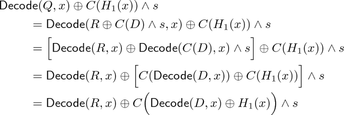
Suppose the receiver uses the strings of a \(\mathsf{PaXoS}\) \(D= (d_1, \ldots , d_m)\) as its OOS inputs, and the parties further interpret their OOS outputs \(Q = (q_1, \ldots , q_m)\) (for the sender) and \(R = (r_1, \ldots , r_m)\) (for the receiver) as \(\mathsf{PaXoS}\) data structures as well. Then we find that the identity \(r_i = q_i \oplus C(d_i)\wedge s\) facilitates the homomorphic properties of \(\mathsf{PaXoS}\):
Suppose the receiver encodes the \(\mathsf{PaXoS}\) D so that \(\mathsf{Decode} (D,x)\) is something “recognizable” (say, x itself) for every item x in his PSI input set. Then the expression above is something that both parties can compute: the receiver computes it as \(\mathsf{Decode} (R,x)\), and the sender computes it as \(\mathsf{Decode} (Q,x) \oplus C(x)\wedge s\).
Hence, we can obtain a PSI protocol by having the sender send \(H( \mathsf{Decode} (Q,x) \oplus C(x) \wedge s)\) for each of her items x. The receiver compares these values to \(H( \mathsf{Decode} (R,y))\) for each of his items y, to determine the intersection.
4.2 Protocol Details
Our full protocol follows the general outline described above, but with some minor technical changes to facilitate the security proof.
One change is that instead of generating a \(\mathsf{PaXoS}\) D where \(\mathsf{Decode} (D,x)=x\), the receiver arranges for \(\mathsf{Decode} (D,x) = H_1(x)\) (for x in his input set) where \(H_1\) is a random oracle. This modification allows the simulator to extract a malicious receiver’s effective input set by observing D (used as input to OOS) and the receiver’s queries to \(H_1\).
Also, instead of sending values of the form \(H( \mathsf{Decode} (Q,x) \oplus C(H_1(x)) \wedge s)\), we have the sender send values of the form \(H( x, \mathsf{Decode} (Q,x) \cdots )\). That is, the item x is included in the clear as an additional argument to H (named \(H_2\) in our construction to avoid confusion with \(H_1\)). Additionally, H (\(H_2\)) is a (non-programmable) random oracle. As above, this allows the simulator to extract a malicious sender’s effective input by observing its random-oracle queries.
The protocol is described formally in Fig. 3.
4.3 Security Analysis
Recall that we are using as our definition an ideal PSI functionality (Fig. 1) that does not strictly enforce the size of a corrupt party’s set. In other words, a corrupt party may provide more items (\(n'\)) than they claim (n). We prove security of our construction without making explicit reference to the relationship between \(n'\) and n. That is, in the proofs below we show that a simulator is able to extract some set (of size polynomial in the security parameter) in the ideal interaction, but the proofs do not explicitly bound the size of these sets.
The protocol contains several parameters \(\ell _1\) and \(\ell _2\) which affect the value of \(n'\) that can be proven. We discuss how to choose these parameters, and the resulting \(n'\) that one obtains, in Sect. 4.4.
Theorem 4
The protocol of Fig. 3 is a secure 2-party PSI protocol against malicious adversaries in the random oracle model.
We prove the theorem in the following two lemmas:

Our \(\mathsf{PaXoS}\)-PSI protocol
Lemma 5
The protocol of Fig. 3 is secure against a malicious receiver in the random oracle model.
Proof
The simulator for a corrupt receiver behaves as follows:
-
It observes the receiver’s input D to OOS, and also observes all of the receiver’s queries to random oracle \(H_1\).
-
The simulator computes \(\tilde{Y} = \{ y \mid y \text { was queried to }H_1 \text { and } \mathsf{Decode} (D,y) = H_1(y) \}\) and sends this to the ideal functionality as the receiver’s effective input.
-
Upon receiving from the ideal functionality the intersection \(Z = X \cap \tilde{Y}\), the simulator simulates the sender’s message M as \(\{ H_2( z, \mathsf{Decode} (R,z)) \mid z \in Z \}\) along with \(|X \setminus Z|\) additional random values.
We prove the indistinguishability of this simulation in the following sequence of hybrids:
-
Hybrid 1: Same as the real protocol interaction, but the simulator maintains a list L of all queries that the adversary makes to random oracle \(H_1\). When the adversary selects its OOS input D, the simulator checks all \(y\in L\) and defines the set \(\tilde{Y} = \{ y \in L \mid \mathsf{Decode} (D,y) = H_1(y) \}\). This hybrid is indistinguishable from the real protocol interaction, since the only difference is in internal bookkeeping information that is not used.
-
Hybrid 2: Same as Hybrid 1, except that immediately after defining \(\tilde{Y}\), the simulator aborts if the honest sender holds an \(x \in X\) where \(\mathsf{Decode} (D,x) = H_1(x)\) but \(x \not \in \tilde{Y}\). It suffices to show that the probability of this artificial abort is negligible.
-
Case \(x \in L\): then \(H_1(x)\) was known at the time \(\tilde{Y}\) was defined. Therefore it is by construction that \(x \in \tilde{Y} \Leftrightarrow \mathsf{Decode} (D,x) =H_1(x)\). In other words, the abort does not happen in this case
-
Case \(x \not \in L\): then \(H_1(x)\) is independent of D, and thus \(\mathsf{Decode} (D,x) = H_1(x)\) with probability \(1/2^{\ell _1}\) where \(\ell _1\) is the output length of \(H_1\).
If \(\ell _1 = \lambda + \log _2 n\) then by a union bound over at most n possible sender’s values \(x \in X\), the abort probability is indeed bounded by \(1/2^\lambda \).
-
-
Hybrid 3: Same as Hybrid 2, except we can rewrite the computation that defines the sender’s message M. Observe that
In particular, the term inside C is zero if and only if \(\mathsf{Decode} (D,x) = H_1(x)\). Furthermore, because of the artificial abort introduced in the previous hybrid, this happens for \(x \in X\) if and only if \(x \in X \cap \tilde{Y}\). Hence, we can rewrite the sender’s message M as:
$$\begin{aligned} M&= \{ H_2( x, \mathsf{Decode} (Q,x) \oplus C(H_1(x))\wedge s ) \mid x \in X \} \\&= \{ H_2( x, \mathsf{Decode} (R,x) ) \mid x \in X \cap \tilde{Y} \} \\&\qquad \cup \, \{ H_2( x, \mathsf{Decode} (R,x) \oplus C(\delta _x)\wedge s ) \mid x \in X \setminus \tilde{Y} \} \end{aligned}$$where the \(\delta _x := \mathsf{Decode} (D,x) \oplus H_1(x)\) values are guaranteed to be nonzero. This hybrid is identical to the previous one, as we have only rewritten the same computation in an equivalent way.
-
Hybrid 4: Same as Hybrid 3, except we replace every term of the form \(H_2( x, \mathsf{Decode} (R,x) \oplus C(\delta _x)\wedge s )\) with random. The two hybrids are indistinguishable by Lemma 1 since \(C(\delta _x)\) are nonzero codewords and hence have Hamming weight at least \(\kappa \). Now note that the sender’s message M is generated as:
$$ M = \{ H_2( x, \mathsf{Decode} (R,x) ) \mid x \in X \cap \tilde{Y} \} \cup \{ m_1, \ldots , m_{|X \setminus \tilde{Y}|} \} $$where each \(m_i\) is uniformly chosen in \(\{0,1\}^{\ell _2}\).
-
Hybrid 5: Same as Hybrid 4, except the simulator no longer artificially aborts in the manner introduced in Hybrid 2. The hybrids are indistinguishable for the same reasoning as before. Now the simulator does not use the items of \(X \setminus \tilde{Y}\) at all. We conclude the proof by observing that this hybrid exactly describes the final ideal-world simulation: the simulator extracts \(\tilde{Y}\), sends it to the ideal PSI functionality, receives \(Z = X \cap \tilde{Y}\), and uses it to simulate the sender’s message M.

Lemma 6
The protocol of Fig. 3 is secure against a malicious sender in the random oracle model.
Proof
The simulator for a corrupt sender behaves as follows:
-
It observes the sender’s input s and output Q from OOS, and also observes all of the sender’s queries to random oracle \(H_2\).
-
When the sender produces protocol message M, the simulator computes
$$\tilde{X} = \{ x \mid x \text { was queried to }H_2\text { and } H_2( x, \mathsf{Decode} (Q,x) \oplus C(H_1(x))\wedge s ) \in M \}$$and sends this to the ideal functionality as the sender’s effective input.
We prove the indistinguishability of this simulation in the following sequence of hybrids:
-
Hybrid 1: Same as the real protocol interaction, except that the simulator observes the sender’s input s and output Q for OOS, and additionally observes all queries made to random oracle \(H_2\). The simulator defines a set L of all the values x such that the adversary queried \(H_2\) on the “correct” value \((x, \mathsf{Decode} (Q,x) \oplus C(H_1(x))\wedge s)\). When the sender gives protocol message M, the simulator defines the set \(\tilde{X} := \{ x \in L \mid H_2(x, \mathsf{Decode} (Q,x) \oplus C(H_1(x))\wedge s ) \in M \}\). This hybrid is identical to the real protocol interaction, since the only change is to record bookkeeping information that is not used.
-
Hybrid 2: Same as Hybrid 1, except the simulator aborts if the honest receiver holds \(y \in Y \setminus \tilde{X} \) where \(H_2(y, \mathsf{Decode} (Q,y) \oplus C(H_1(y)) \wedge s ) \in M\). There are two cases for why such a y may not be in \(\tilde{X}\):
-
Case \(y \in L\): then the value \(H_2(y, \mathsf{Decode} (Q,y) \oplus C(H_1(y)) \wedge s)\) was defined at the time \(\tilde{X}\) was computed, and y was excluded because the correct value was not in M. The simulator will never abort in this case.
-
Case \(y \not \in L\): the adversary never queried \(H_2\) at \(H_2(y, \mathsf{Decode} (Q,y) \oplus C(H_1(y)) \wedge s)\) before sending M, so this output of \(H_2\) is random and independent of M. The probability that this \(H_2\)-output appears in M is thus \(|M|/2^{\ell _2}\) where \(\ell _2\) is the output length of \(H_2\).
Overall, the probability of such an artificial abort is bounded by \(n|M|/2^{\ell _2} \le n^2 / 2^{\ell _1} \le 1/2^\lambda \) (since \(\ell _1 < \ell _2\) and \(\ell _1 \ge \lambda +2\log n\)). Hence the two hybrids are indistinguishable.
-
-
Hybrid 3: Same as Hybrid 2, except we change the way the honest receiver’s output is computed. In Hybrid 2, the honest receiver computes output as in the protocol specification:
$$ \{ y \in Y \mid H_2(y, \mathsf{Decode} (R,y)) \in M \} $$In this hybrid we make the honest receiver compute its output as, simply, \(\tilde{X} \cap Y\). These two expressions are in fact equivalent, from the definition of \(\tilde{X}\), the artificial abort introduced in the previous expression, and the equivalence of \(\mathsf{Decode} (R,y)\) and \(\mathsf{Decode} (Q,y) \oplus C(H_1(y))\wedge s\) discussed in the previous proof.
-
Hybrid 4: Same as Hybrid 3, except we remove the artificial abort condition that was introduced in Hybrid 2. The hybrids are indistinguishable for the same reason as before. Note that in this hybrid, the simulator does not use the honest receiver’s input Y except to compute the receiver’s final output. We conclude the proof by observing that this hybrid exactly describes the ideal world simulation: The simulator observes s, Q and the sender’s oracle queries to determine a set \(\tilde{X}\). It sends \(\tilde{X}\) to the ideal functionality and \(\tilde{X} \cap Y\) is delivered to the receiver.
4.4 Choosing Parameters
The protocol contains several parameters:
-
A linear binary code \(C: \{0,1\}^{\ell _1} \rightarrow \{0,1\}^t\).
-
Random oracle output lengths \(\ell _1, \ell _2\).
As shown in the security proof, the following facts must be true in order for security to hold:
-
C must have minimum distance at least \(\kappa \) (the computational security parameter).
-
\(\ell _1, \ell _2 \ge \lambda + 2\log n\), where \(\lambda \) is the statistical security parameter.
However, the parameters \(\ell _1, \ell _2\) also have an effect on the size of the corrupt party’s set, as extracted by the simulator. In particular, increasing these values causes the protocol to more tightly enforce the size (\(n'\)) of the corrupt party’s input set.
We note that the communication cost of the protocol is roughly \(\ell _2\) bits per item from the sender and roughly t bits per item from the receiver (sent as part of the OOS protocol, where t is the length of the code used in the OOS protocol).
Semi-honest security. To instantiate our protocol for semi-honest security, it is enough to set \(\ell _1 = \ell _2 = \lambda + 2\log n\), the minimum possible value for security. The issue of extracting a corrupt party’s input, which involves further increasing \(\ell _1, \ell _2\), is not relevant in the semi-honest case.
It therefore suffices to identify linear (binary) codes with suitable minimum distance, for the different values of \(\ell _1\) that result. We identify good choices in Fig. 4, all of which are the result of concatenating a Reed-Solomon code with a small (optimal) binary code.

Parameters for semi-honest instantiation of \(\mathsf{PaXoS}\)-PSI, with \(\kappa =128\) and \(\lambda =40\).
Malicious sender’s set size. Consider a malicious sender and recall how the simulator extracts an effective input for that sender. The sender gives protocol message M and the simulator extracts via
where L is the set of x values such that the adversary has queried \(H_2(x,\cdot )\). The protocol limits the protocol message M to have n items, but still \(\tilde{X}\) may have many more than n items if the adversary manages to find collisions in \(H_2\). If we set \(\ell _2\) (the output length of \(H_2\)) to be \(2\kappa \), then collisions are negligibly likely and indeed \(|\tilde{X}| \le n\) except with negligible probability.
While it is possible to set \(\ell _2 < 2\kappa \), doing so has less impact on the protocol than the other parameters (\(\ell _1\) and hence t). One can reduce \(\ell _2\) only very slightly before the adversary can find a very large amount (e.g., superlinear in n) of collisions. For these reasons, we recommend setting \(\ell _2 = 2\kappa \) in our malicious instantiation.
Malicious receiver’s set size. Consider a malicious receiver and recall how the simulator extracts an effective input for that receiver. The simulator observes the receiver’s input D (a \(\mathsf{PaXoS}\)) to OOS and also observes all queries made to the random oracle \(H_1\). Then the simulator extracts via:
where L is the set of queries made to \(H_1\). The question becomes: as a function of |D| and \(\ell _1\) (the output length of \(H_1\)), what is an upper bound on the number of items in \(\tilde{Y}\)?
In the full version [27] we prove the following, using an information-theoretic compression argument:
Claim
Suppose an adversary makes q queries to random oracle \(H_1\) with output length \(\ell _1\) and then generates a \(\mathsf{PaXoS}\) D of size m (hence \(m \ell _1\) bits) total. Fix a value \(n'\) and let \(\mathcal E\) denote the event that \(\mathsf{Decode} (D,y) = H_1(y)\) for at least \(n'\) values y that were queried to \(H_1\). Then
The idea behind the proof is that if a \(\mathsf{PaXoS}\) D happens to encode many \(H_1(y)\) values, then D could be used to compress \(H_1\). However, this is unlikely due to \(H_1\) being a random object and therefore incompressible.
For reference, we have computed some concrete parameter settings so that \(\Pr [\mathcal E] < 2^{-40}\) (the probability that the simulator extracts more than \(n'\) items). The values are given in Fig. 5. We consider an adversary making \(q=2^{128}\) queries to \(H_1\), which is rather conservative (in terms of security). In practice significantly smaller parameters may be possible.Footnote 4 Note that if the \(\mathsf{PaXoS}\) has size m, then a compression argument such as the one we use only starts to apply when \(n' > m\). Hence all of our bounds are expressed as \(n' = cm\) where \(c>1\) is a small constant.
Recall that \(\ell _1\) is the input length to the linear code C, so increasing it has the effect of increasing t (the codeword length) as well. We include good choices of codes (achieving minimum distance \(\kappa =128\)) in the figure as well.

Parameters for malicious \(\mathsf{PaXoS}\)-PSI with \(\kappa =128\) and \(\Pr [{\text {simulator extracts}} > n' {\text { items from malicious receiver}}] < 1/2^{40}\), where adversary makes \(2^{128}\) queries to \(H_1\).
5 Garbled Cuckoo Table
We introduce a new approach for \(\mathsf{PaXoS}\) that enjoys the best of all worlds: it has the same asymptotic encoding and decoding costs as a garbled Bloom filter, but with constant rate (e.g., \(\sim 1/(2+\epsilon )\)) rather than a \(O(1/\lambda )\) rate. Furthermore, it has a linear time construction, just like the modified Bloomier filter of [3], but with the advantage of having the hash function(s) independent of the keys/values.
5.1 Overview
Our construction uses ideas from both garbled Bloom filters as well as Cuckoo hashing. Recall that in Cuckoo hashing, it is typical to have only 2 hash functions \(h_1, h_2\), where an item x is associated with positions \(h_1(x)\) and \(h_2(x)\) in the data structure.
So as a starting point, consider a garbled Bloom filter with just 2 hash functions rather than \(\lambda \). Such a data structure corresponds to the decoding function \(\mathsf{Decode} (D,x) = d_{h_1(x)} \oplus d_{h_2(x)}\).Footnote 5 (Using the PaXoS key-value mapping terminology of Sect. 3.2, the vector \(\varvec{v}(x)\) has only two non-zero entries, in locations \(h_1(x)\) and \(h_2(x)\).) Given n key-value pairs \((x_i,y_i)\), how can we generate a data structure \(D = (d_1, \ldots , d_m)\) that encodes them in this way?
An important object in analyzing our construction is the cuckoo graph. The vertices in the cuckoo graph are numbered 1 through m, and correspond to the positions in the data structure D. The (undirected) edges of the graph correspond to items that are meant to be inserted. An item x corresponds to the edge \(\{h_1(x), h_2(x)\}\). (The graph may contain self-loops and repeated edges.) We refer to such graphs with m vertices and n edges as (n, m)-cuckoo graphs and note that the distribution over such graphs is independent of X. We write \(G_{h_1,h_2,X}\) to refer to the specific (n, m)-cuckoo graph corresponding to a particular set of hash functions and keys X. All properties of our \(\mathsf{PaXoS}\) can be understood in terms of properties of random (n, m)-cuckoo graphs.
In the simplest case, suppose that \(G_{h_1,h_2,X}\) happens to be a tree. Our goal is to encode the items X into the data structure D. Each node g in the graph corresponds to a row \(d_g\) of D. Then we can do this encoding in linear time as follows: We choose an arbitrary root vertex r of the tree and set \(d_r\) of the data structure arbitrarily. We then traverse the tree, say, in DFS or BFS order. Each time we visit a vertex j for the first time, we set its corresponding value \(d_j\) in the data structure, to agree with the edge we just traversed. This is done as follows.
Recall that each edge ij corresponds to a key-value pair (x, y) in the sense that \(\{i,j\} = \{h_1(x),h_2(x)\}\) and our goal is to arrange that \(d_i \oplus d_j = y\). As we cross an edge from i to j in the traversal, we have the invariant that position \(d_i\) in the data structure has been already fixed but \(d_j\) is still undefined. Hence, we can always set \(d_j := d_i \oplus y\).
Handling Cycles. When \(m = O(n)\), corresponding to a \(\mathsf{PaXoS}\) of constant rate, the corresponding Cuckoo graph is unlikely to be acyclic [10]. In this case the encoding procedure that we just outlined does not work, since when the graph traversal closes a circuit it encounters a vertex whose value has already been defined and cannot be set to satisfy the constraint imposed by the current edge.
We can handle acyclic Cuckoo graphs by adding \(d+\lambda \) additional entries to the data structure D. We first describe an analysis where d is an upper bound on the size \(\chi \) of the 2-core of the graph, and then an analysis where d is an upper bound on the cyclomatic number \(\sigma \) of the graph. (These bounds are \(O((\log n)^{1+\omega (1)})\) and \(\log n\), respectively.) We recall below the definitions of both these values, and note that \(\sigma < \chi \) always.
The 2-core of a graph is the maximum subgraph where each node has degree at least 2 (namely, the subgraph containing all cycles, as well as all paths connecting cycles). We use \(\chi \) to denote the number of edges in the 2-core. The cyclomatic number of a graph is the minimum number of edges to remove to leave an acyclic graph. Equivalently, it is the number of non-tree edges (back edges) in a DFS traversal of the graph. We use \(\sigma \) to denote the cyclomatic number. The cyclomatic number is equal to the minimal number of independent cycles in the graph, and is therefore smaller than or equal to the number of cycles. It is also always strictly less than the size of the 2-core.
The construction. D will be structured as \(D = L \Vert R\), where \(|L|=m\) (the number of vertices in the Cuckoo graph) and \(|R| = d + \lambda \). Each decoding/constraint vector \(\varvec{v}(x)\) then has the form \(\varvec{v}(x) = \varvec{l}(x) \Vert \varvec{r}(x)\), where \(\varvec{l}(x)\) determines the positions of L to be XOR’ed and \(\varvec{r}(x)\) determines the positions of R to be XOR’ed. We will let L correspond to the simple Cuckoo hashing idea above, so each \(\varvec{l}(x)\) vector is zeroes everywhere except for two 1s. We will let \(\varvec{r}(x)\) be determined uniformly at random for each x (similar to the random matrix construction of a \(\mathsf{PaXoS}\)).
To encode n key-value pairs into the data structure in this way, first consider the system of linear equations induced by the constraints \(\langle \varvec{v}(x_i) , D \rangle = y_i\), restricted to only the \(\chi \) items (edges) in the 2-core. (Once we set values that encode the items in the 2-core, we will be able to encode the other items using graph traversal as in an acyclic graph.) These constraints refer to a vertex u of G only if that vertex is in the 2-core. We get \(\chi \) equations over \(m+d+\lambda \) variables, where the coefficients of the last \(d+\lambda \) variables (the \(\varvec{r}(x)\) part) are random. If we set d to be an upper bound on \(\chi \) then we get that the system has a solution with probability \(1-2^{-\lambda }\).
So, using a general-purpose linear solver we can find values for R and for the subset of L corresponding to the vertices in the 2-core, that satisfies these constraints. This can be done in \(O((d+\lambda )^3)\) time. For vertices u outside of the 2-core, the value of \(d_u\) in the data structure remains undefined. But after removing the 2-core, the rest of the graph is such that these values in the data structure can be fixed according to a tree traversal process:
Every edge not in the 2-core can be oriented away from all cycles (if an edge leads to a cycle in both directions, then that edge would have been part of the 2-core). We traverse those edges following the direction of their orientation. Let edge \(i \rightarrow j\) correspond to a key-value pair (x, y). Let \(d_j\) denote the position in D (in its “L region”) corresponding to vertex j. By our invariant, \(d_j\) is not yet fixed when we traverse \(i \rightarrow j\). Yet it is the only undefined value relevant to the constraint \(\langle \varvec{v}(x), D \rangle = y\), so we can satisfy the constraint by solving for \(d_j\). Hence with a linear pass over all remaining items, we finish constructing the data structure D.
The total cost of encoding is therefore \(O((d+\lambda )^3 + n\lambda )\). We explained above that we can set d to be an upper bound on the size of the 2-core.Footnote 6 As we shall see (in Sect. 5.2), it is possible to set d to be the cyclomatic number of the Cuckoo graph, which is logarithmic in n. Therefore the dominating part of the expression is \(n\lambda \).
5.2 Details
The garbled-cuckoo construction is presented formally in Fig. 6.

Garbled Cuckoo \(\mathsf{PaXoS}\)
Analysis & Costs. In the full version of the paper [27] we show that the number \(\sigma \) of cycles is smaller than \(\log n +O(1)\) except with negligible probability. Therefore we can set \(d=(1+\varepsilon )\log n\).Footnote 7 This bound also applies to the cyclomatic number (which is always smaller than or equal to the number of cycles). Theorem 7 shows that it is sufficient to set d to be equal to this upper bound on the cyclomatic number.
Recall that each item is mapped to a row \(\varvec{l}(x_i) \Vert \varvec{r}(x_i)\) which contains an \(\varvec{l}(x_i)\) part with two 1 entries, and a random binary vector \(\varvec{r}(x_i)\) of length \(\lambda +d\). We set \(\lambda = 40\), and therefore for all practical input sizes we get that \(d < \lambda \). We conclude that the number of 1 entries in the row vector is \(O(\lambda )\).
The encoding processes each of n edges once during the traversal. The computation involves XORing the locations pointed to by 1 entries in the row. The overhead of encoding all rows is \(O(n\lambda )\). The decoding of a single item involves XORing the rows pointed by the two rows to which it is mapped, and is \(O(\lambda )\).
Theorem 7
When setting \(d=(1+\varepsilon )\log n\), the garbled cuckoo \(\mathsf{PaXoS}\) of Fig. 6 with parameter \(\lambda \) is a \((n,m,\epsilon +2^{-\lambda })\)-\(\mathsf{PaXoS}\) where
Proof
As discussed above, we use here an upper bound d for the cyclomatic number of the graph. Setting the bound to \(d=(1+\varepsilon )\log n\) works excepts with a negligible failure probability.
The proof bounds the probability that the \(\mathsf{Encode} \) algorithm fails to satisfy the linear constraints \(\langle \varvec{v}(x_i), D \rangle = y_i\) for every i. For items \(x_i\) that do not correspond to edges in the 2-core, Step 4 of \(\mathsf{Encode} \) satisfies the appropriate linear constraint, by construction. For items in the 2-core, their linear constraints are fixed all at once in Step 3 of \(\mathsf{Encode} \). Hence, the construction only fails if Step 3 fails. Step 3 solves for the following system of equations:
We interpret \(\{ \varvec{l}(x_i) \Vert \varvec{r}(x_i)\}_{x_i \in \tilde{E}}\) as a matrix \(M_L | M_R\) where the first m columns (i.e., \(M_L\)) are \(\{ \varvec{l}(x_i)\}_{x_i \in \tilde{E}}\) and the remaining \(d+\lambda \) columns (i.e., \(M_R\)) are \(\{ \varvec{r}(x_i)\}_{x_i \in \tilde{E}}\). We therefore ask whether the rows of the matrix \(M_L | M_R\) are linearly independent.
There are up to d cycles in the graph, denoted as \(C_1,\ldots ,C_d\). Let us focus on the matrix \(M_L\), and more specifically on the rows corresponding an arbitrary cycle \(C_i\) (each of these rows has two 1 entries, at the locations of the vertices touching the corresponding edge). It is easy to see that there is a single linear combination \(D_i\) of these rows which is 0 (the XOR of all these rows). Any linear combination of \(D_1,\ldots ,D_d\) is 0, and these are the only linear combinations of rows which are equal to 0. Therefore there are at most \(2^d\) such combinations and the kernel of \(M_L\) is of dimension at most d.
Our goal is to find the probability of the existence of a zero linear combination of the rows of \(M_L|M_R\), rather than the rows of \(M_L\) alone. Since in \(M_R\) each row contains \(d+\lambda \) random bits, this probability is at most \(2^{-\lambda }\). \(\square \)
5.3 Comparison
Our construction shares many features with garbled Bloom filters (GBF), and indeed is somewhat inspired by them. Both our construction and GBF involve probing about the same number of positions per item (\(\frac{\lambda +\chi +2}{2}\) in average vs. \(O(\lambda )\)), however we are able to obtain constant rate while GBFs have rate \(O(1/\lambda )\). We point out that GBFs inherit from standard Bloom filters their support for fully online insertion; that is, their analysis proves that items can be added to a GBF in any order. Our approach builds the data structure in a very particular order (according to a global tree or tree-like structure of a graph). This qualitative difference seems important for achieving constant rate.
We also use much of the analysis techniques and terminology from cuckoo hashing (especially cuckoo hashing with a stash). However, one important difference with typical cuckoo hashing is that our construction can handle multiple cycles in a connected component of the cuckoo graph. Indeed, usual cuckoo hashing (without a stash) succeeds if each connected component of the graph has at most one cycle. The items in a cycle can be handled by arbitrarily assigning an orientation to the cycle, and assigning each edge (item) to its forward endpoint (position in the table). In our case, if some items form a cycle, their corresponding constraint vectors become linearly dependent and we cannot solve the system of linear equations. In general, our approach has a larger class of subgraphs which present a “barrier” to the process (where graphs with only 1 cycle are a barrier for us but not for standard cuckoo hashing), making the analyses slightly different.
5.4 An Alternative Construction
In full version of the paper [27] we describe a modified construction which is based on a DFS traversal of the graph, and has a similar overhead to the construction described in this section.
6 A Theoretical Comparison
In Table 1 we show the theoretical communication complexity of our protocol compared with the Diffie-Hellman based PSI, the KKRT protocol [19] and the SpoT protocol [26] in the semi-honest setting, and the Rindal-Rosulek [34] and Ghosh-Nilges [8] protocols in the malicious setting. This comparison measures how much communication the protocols require on an idealized network where we do not care about protocol metadata, realistic encodings, byte alignment, etc. In practice, data is split up into multiples of bytes (or CPU words), and different data is encoded with headers, etc.—empirical measurements of such real-world costs are given later in Sect. 7.
PaXoS PSI has linear communication complexity. Let us clarify our claim of “linear communication.” Consider the insecure intersection protocol where Alice sends H(x) for every x in her set. H could have output length equal to security parameter, giving \(O(n\cdot \kappa )\) communication. But with semi-honest parties H can also have output length as small as \(\lambda +2\log (n)\) to ensure correctness with probability \(1-1/2^\lambda \). When viewed this way, it looks like the protocol has complexity \(O(n \log n)\)! However, if \(1/2^\lambda \) is supposed to be negligible then certainly \(\log n \ll \lambda \), so one could still write \(O(n\cdot \lambda )\).
If we let L be a length that depends on the security parameters and \(\log n\) (which is inherent to all intersection protocols, secure or not), then insecure PSI and PaXoS-PSI have complexity \(O(L\cdot n)\), while previous OT-based malicious PSI [34] has complexity \(O(L\cdot n\log n)\) or even \(O(L\cdot n\kappa )\) [33]. For comparison, semi-honest KKRT [19] protocol has complexity \(\omega (L\cdot n)\) (from the stash growing as \(\omega (1)\)) and semi-honest PRTY [26] has complexity \(O(L\cdot n)\).
In [26] and in this work, L can depend on the security parameter alone, leading to a \(O(n\cdot \kappa )\) communication, which we would characterize as linear in n. But when choosing concrete parameters (just like in the insecure protocol) L can be made smaller by involving a \(O(\log n)\) term. Again, this is endemic to all intersection protocols.
7 Implementation and Evaluation
7.1 Implementation Details
We now present a comparison based on implementations of all protocols. We used the implementation of KKRT [19], RR [34], HD-PSI, spot-low, spot-fast [26] from the open source-codeFootnote 8 provided by the authors.
We evaluate the DH-PSI protocol, instantiated with two different elliptic curves: Curve25519 [2] and Koblitz-283. Curve25519 elements are 256 bits while K-283 elements are 283 bits. Using the Miracl library, K-283 operations are faster than Curve25519, giving us a tradeoff of running time vs. communication for DH-PSI.
All OT-based PSI protocols [19, 26, 34] (including our protocols) require the same underlying primitives: a Hamming correlation-robust function H, a pseudorandom function F, and base OTs for OT extension. We instantiated these primitives exactly as in previous protocols (e.g, KKRT, RR): both H and F instantiated using AES, and base OTs instantiated using Naor-Pinkas [22]. We use the implementation of base OTs from the libOTe libraryFootnote 9. All protocols use a computational security parameter of \(\kappa = 128\) and a statistical security parameter \(\lambda = 40\).
For our own protocols, we implemented two variants of our \(\mathsf{PaXoS}\). We implemented the DFS traversal of the cuckoo graph (see the full version [27]) using the boost library. We used additional libraries linbox, gmp, ntl, givaro iml, blas for solving systems for linear equations and generating the required concatenated linear codes needed for the 2-core based variant of Sect. 5. We use 2n bins in our DFS based \(\mathsf{PaXoS}\), and 2.4n bin in our 2-core based variant.
7.2 Experimental Setup
We performed a series of benchmarks on the Amazon web services (AWS) EC2 cloud computing service. We used the M5.large machine class with 2.5 GHz Intel Xeon and 8 GB RAM.6
We tested the protocols over three different network settings: LAN – two machines in the same region (N.Virginia) with bandwidth 4.97 GiB/s; WAN1 – one machine in N.Virginia and the other in Oregon with bandwidth 155 MiB/s; and WAN2 – one machine in N.Virginia and the other in Sydney with bandwidth 55 MiB/s. All experiments are performed with a single thread (with an additional thread used for communication). Find the result of the WAN2 setting in the full version of the paper [27].
7.3 Experimental Results
A detailed benchmark for set sizes \(n = \{2^{12}, 2^{16}, 2^{20}\}\) is given in Table 2.
Semi-honest PSI Comparison. Our best protocol in terms of communication is PaXoS-DFS. The communication of this protocol is less than 10% larger than that of KKRT [19], and slightly more than twice the communication of SpOT-low.
Our best protocol in terms of run time is PaXoS 2-core. In the LAN setting for \(2^{20}\) inputs, it runs only 18% slower than KKRT. In the two WAN settings it is about 80% slower.
Malicious PSI Comparison. The communication of both implementations of our protocol is better than that of RR. For \(2^{20}\) items, PaXoS-DFS uses almost 8 times less communication, and PaXoS 2-core uses 6.5 less communication.
In terms of run time, PaXoS 2-core is faster than RR by a factor of about 2.5 on a LAN, and factors of 3.7–4 in the two WAN settings. The larger improvement in the WAN settings is probably due to the larger effect that the improvement in the communication has over a WAN.
Semi-honest vs. Malicious. In both our implementations of PaXoS the malicious implementation uses only about 25% more communication than the semi-honest implementation. In the LAN setting, our malicious protocols run about 4% slower than our corresponding semi-honest protocols.
Notes
- 1.
A hash table is a simple key-value mapping, but it encounters issues such as collisions. More importantly for our application, a hash table explicitly reveals whether an item is encoded in it and therefore has a privacy leakage.
- 2.
When defining the cost of encoding and decoding we ignore the length (m) of the y-values.
- 3.
I.e., \(\varvec{v}^H(x) = H(x)\) where H is a random oracle with m output bits.
- 4.
For example, considering an adversary who makes \(q=2^{80}\) queries to \(H_1\) leads to \(\ell _1\) in the range of 70 to 90, and codeword length t in the range of 460 to 510.
- 5.
For now, we ignore the case where \(h_1(x) = h_2(x)\).
- 6.
Such an upper bound for the case of Cuckoo hashing can be derived from [24, Lemma 3.4], but that analysis assumes that the graph has 8n edges, and shows that an upper bound of size d fails with probability \(n/2^{-\varOmega (d)}\). Therefore we must set \(d=(\log n)^{1+\epsilon }\) to get a negligible failure probability.
- 7.
The parameter \(\varepsilon \) used here is independent of the parameter \(\epsilon \) used in Cuckoo hashing.
- 8.
- 9.
References
Asharov, G., Lindell, Y., Schneider, T., Zohner, M.: More efficient oblivious transfer and extensions for faster secure computation. In: ACM CCS, pp. 535–548 (2013)
Bernstein, D.J.: Curve25519: new Diffie-Hellman speed records. In: Yung, M., Dodis, Y., Kiayias, A., Malkin, T. (eds.) PKC 2006. LNCS, vol. 3958, pp. 207–228. Springer, Heidelberg (2006). https://doi.org/10.1007/11745853_14
Charles, D., Chellapilla, K.: Bloomier filters: a second look. In: Halperin, D., Mehlhorn, K. (eds.) ESA 2008. LNCS, vol. 5193, pp. 259–270. Springer, Heidelberg (2008). https://doi.org/10.1007/978-3-540-87744-8_22
Chen, H., Huang, Z., Laine, K., Rindal, P.: Labeled PSI from fully homomorphic encryption with malicious security. In: Proceedings of the 2018 ACM SIGSAC Conference on Computer and Communications Security, CCS 2018, Toronto, ON, Canada, 15–19 October 2018, pp. 1223–1237 (2018)
Dong, C., Chen, L., Wen, Z.: When private set intersection meets big data: an efficient and scalable protocol. In: ACM CCS 2013, pp. 789–800 (2013)
Even, S., Goldreich, O., Lempel, A.: A randomized protocol for signing contracts. Commun. ACM 28, 637–647 (1985)
Freedman, M.J., Nissim, K., Pinkas, B.: Efficient private matching and set intersection. In: Cachin, C., Camenisch, J.L. (eds.) EUROCRYPT 2004. LNCS, vol. 3027, pp. 1–19. Springer, Heidelberg (2004). https://doi.org/10.1007/978-3-540-24676-3_1
Ghosh, S., Nilges, T.: An algebraic approach to maliciously secure private set intersection. In: Ishai, Y., Rijmen, V. (eds.) EUROCRYPT 2019. LNCS, vol. 11478, pp. 154–185. Springer, Cham (2019). https://doi.org/10.1007/978-3-030-17659-4_6
Goldreich, O.: Foundations of Cryptography, Volume 2: Basic Applications. Cambridge University Press, Cambridge (2004)
Havas, G., Majewski, B.S., Wormald, N.C., Czech, Z.J.: Graphs, hypergraphs and hashing. In: van Leeuwen, J. (ed.) WG 1993. LNCS, vol. 790, pp. 153–165. Springer, Heidelberg (1994). https://doi.org/10.1007/3-540-57899-4_49
Hazay, C., Lindell, Y.: Efficient protocols for set intersection and pattern matching with security against malicious and covert adversaries. J. Cryptology 23(3), 422–456 (2010). https://doi.org/10.1007/s00145-008-9034-x
Huang, Y., Evans, D., Katz, J.: Private set intersection: are garbled circuits better than custom protocols? In: NDSS (2012)
Huberman, B.A., Franklin, M.K., Hogg, T.: Enhancing privacy and trust in electronic communities. In: EC, pp. 78–86 (1999)
Ion, M., et al.: Private intersection-sum protocol with applications to attributing aggregate ad conversions. ePrint Archive 2017/738 (2017)
Ishai, Y., Kilian, J., Nissim, K., Petrank, E.: Extending oblivious transfers efficiently. In: Boneh, D. (ed.) CRYPTO 2003. LNCS, vol. 2729, pp. 145–161. Springer, Heidelberg (2003). https://doi.org/10.1007/978-3-540-45146-4_9
Jarecki, S., Liu, X.: Efficient oblivious pseudorandom function with applications to adaptive OT and secure computation of set intersection. In: Reingold, O. (ed.) TCC 2009. LNCS, vol. 5444, pp. 577–594. Springer, Heidelberg (2009). https://doi.org/10.1007/978-3-642-00457-5_34
Kirsch, A., Mitzenmacher, M., Wieder, U.: More robust hashing: cuckoo hashing with a stash. SIAM J. Comput. 39(4), 1543–1561 (2009)
Kolesnikov, V., Kumaresan, R.: Improved OT extension for transferring short secrets. In: Canetti, R., Garay, J.A. (eds.) CRYPTO 2013. LNCS, vol. 8043, pp. 54–70. Springer, Heidelberg (2013). https://doi.org/10.1007/978-3-642-40084-1_4
Kolesnikov, V., Kumaresan, R., Rosulek, M., Trieu, N.: Efficient batched OPRF with applications to PSI. In: ACM CCS (2016)
Meadows, C.: A more efficient cryptographic matchmaking protocol for use in the absence of a continuously available third party. In: IEEE S&P (1986)
Meadows, C.A.: A more efficient cryptographic matchmaking protocol for use in the absence of a continuously available third party. In: Proceedings of the 1986 IEEE Symposium on Security and Privacy, Oakland, California, USA, 7–9 April 1986, pp. 134–137 (1986)
Naor, M., Pinkas, B.: Efficient oblivious transfer protocols. In: Kosaraju, S.R. (ed.) 12th SODA, pp. 448–457. ACM-SIAM, January 2001
Orrú, M., Orsini, E., Scholl, P.: Actively secure 1-out-of-N OT extension with application to private set intersection. In: Handschuh, H. (ed.) CT-RSA 2017. LNCS, vol. 10159, pp. 381–396. Springer, Cham (2017). https://doi.org/10.1007/978-3-319-52153-4_22
Pagh, A., Pagh, R.: Uniform hashing in constant time and optimal space. SIAM J. Comput. 38(1), 85–96 (2008)
Pagh, R., Rodler, F.F.: Cuckoo hashing. J. Algorithms 51(2), 122–144 (2004)
Pinkas, B., Rosulek, M., Trieu, N., Yanai, A.: SpOT-light: lightweight private set intersection from sparse OT extension. In: Boldyreva, A., Micciancio, D. (eds.) CRYPTO 2019. LNCS, vol. 11694, pp. 401–431. Springer, Cham (2019). https://doi.org/10.1007/978-3-030-26954-8_13
Pinkas, B., Rosulek, M., Trieu, N., Yanai, A.: PSI from PaXoS: fast, malicious private set intersection. ePrint archive 2020/193 (2020)
Pinkas, B., Schneider, T., Tkachenko, O., Yanai, A.: Efficient circuit-based PSI with linear communication. In: Ishai, Y., Rijmen, V. (eds.) EUROCRYPT 2019. LNCS, vol. 11478, pp. 122–153. Springer, Cham (2019). https://doi.org/10.1007/978-3-030-17659-4_5
Pinkas, B., Schneider, T., Weinert, C., Wieder, U.: Efficient circuit-based PSI via cuckoo hashing. In: Nielsen, J.B., Rijmen, V. (eds.) EUROCRYPT 2018. LNCS, vol. 10822, pp. 125–157. Springer, Cham (2018). https://doi.org/10.1007/978-3-319-78372-7_5
Pinkas, B., Schneider, T., Zohner, M.: Faster private set intersection based on OT extension. In: USENIX 2014, pp. 797–812 (2014)
Pinkas, B., Schneider, T., Zohner, M.: Scalable private set intersection based on OT extension. ACM Trans. Priv. Secur. 21(2), 7:1–7:35 (2018)
Rabin, M.O.: How to exchange secrets with oblivious transfer. ePrint Archive 2005/187 (2005)
Rindal, P., Rosulek, M.: Improved private set intersection against malicious adversaries. In: Coron, J.-S., Nielsen, J.B. (eds.) EUROCRYPT 2017. LNCS, vol. 10210, pp. 235–259. Springer, Cham (2017). https://doi.org/10.1007/978-3-319-56620-7_9
Rindal, P., Rosulek, M.: Malicious-secure private set intersection via dual execution. In: Thuraisingham, B.M., Evans, D., Malkin, T., Xu, D. (eds.) ACM CCS 2017, pp. 1229–1242. ACM Press, October 2017
Shamir, A.: On the power of commutativity in cryptography. In: de Bakker, J., van Leeuwen, J. (eds.) ICALP 1980. LNCS, vol. 85, pp. 582–595. Springer, Heidelberg (1980). https://doi.org/10.1007/3-540-10003-2_100
Author information
Authors and Affiliations
Corresponding authors
Editor information
Editors and Affiliations
Rights and permissions
Copyright information
© 2020 International Association for Cryptologic Research
About this paper

Cite this paper
Pinkas, B., Rosulek, M., Trieu, N., Yanai, A. (2020). PSI from PaXoS: Fast, Malicious Private Set Intersection. In: Canteaut, A., Ishai, Y. (eds) Advances in Cryptology – EUROCRYPT 2020. EUROCRYPT 2020. Lecture Notes in Computer Science(), vol 12106. Springer, Cham. https://doi.org/10.1007/978-3-030-45724-2_25
Download citation
DOI: https://doi.org/10.1007/978-3-030-45724-2_25
Published:
Publisher Name: Springer, Cham
Print ISBN: 978-3-030-45723-5
Online ISBN: 978-3-030-45724-2
eBook Packages: Computer ScienceComputer Science (R0)
