
Abstract
The development of intravital microscopy has provided unprecedented capacity to study the tumor microenvironment in live mice. The dynamic behavior of cancer, stromal, vascular, and immune cells can be monitored in real time, in situ, in both primary tumors and metastatic lesions, allowing treatment responses to be observed at single cell resolution and therapies tracked in vivo. These features provide a unique opportunity to elucidate the cellular mechanisms underlying the biology and treatment of cancer. We describe here a method for imaging the microenvironment of subcutaneous tumors grown in mice using intravital microscopy.
Access provided by CONRICYT – Journals CONACYT. Download protocol PDF
Key words
- Tumor microenvironment
- Intravital microscopy
- Multiphoton imaging
- Confocal imaging
- Mouse models
- Subcutaneous tumors
1 Introduction
The tumor microenvironment (TME) is a complex structure comprising both malignant and non-malignant cells, often supported by a dense matrix of extracellular protein and a disorganized network of blood vessels [1–3]. Indeed, cancer biology is increasingly being viewed through the lens of the TME as a tissue. Within the TME, various behaviors of noncancer cells such as inflammatory and immune cells and their interactions with malignant cells are now recognized as “hallmarks of cancer” [4]. Increasingly, new treatments are being developed to target noncancer cells within the TME, such as the antiangiogenesis and immunotherapy classes of medicines [5–8]. Developing these therapies effectively, however, is predicated upon a deep appreciation of how cancer and noncancer cells function and interact within the TME. Unfortunately, until recently, our ability to study cellular behavior within the TME was limited to snapshots in time provided by biochemical or histological analyses.
Microscopic imaging of the TME in vivo using intravital microscopy (IVM) represents a powerful new technique for overcoming this limitation [9–11]. IVM enables the visualization of fluorescently labeled cells within the TME over space and time. With IVM, individual cancer and noncancer cells can be tracked, their interactions with one another analyzed, and their behavior studied—all in live mice [12, 13]. IVM can reveal cellular responses within the TME relevant to most, if not all hallmarks of cancer, from deregulated cell growth to metastasis to angiogenesis to the recruitment of inflammatory cells [14]. Treatment responses can be monitored at the cellular level, and indeed many therapies themselves can be labeled and tracked at high resolution [15]. Moreover, as Turnkey systems are now available from a variety of commercial venders, IVM is an accessible technique for most modern cancer biology laboratories [16].
The general principle behind IVM is that cells labeled with fluorescent reporters, typically conjugated to an antibody injected into the mouse or genetically expressed in a reporter mouse strain, can be visualized in situ by exciting fluorophores within the tumor and collecting and separating the specific fluorescence signal from the out-of-focus light. Accomplishing this with sufficient spatial and temporal resolution to observe individual moving cells, without damaging the tissue, is typically achieved using a scanning or spinning-disk confocal fluorescence microscope or a multiphoton fluorescence microscope, equipped with a variety of detectors and filters. In general, confocal platforms are cheaper, easier to use, and more amenable to multiplexing (visualizing multiple markers in the same animal), but limited by an imaging depth of approximately 70–100 μm in most tumors. Thus, although the tumor surface, its vasculature and the leukocytes within are easily imaged using a confocal platform, limitations in imaging depth prevent clear visualization of the TME much beyond the surface. In contrast, multiphoton microscopes provide an imaging depth of 300–500 μm in most tumors, which enables deeper and more complete imaging of the TME. The downside of this platform, however, is its expense and operational complexity.
Below we provide a detailed method for performing IVM of the microenvironment in transplantable tumors established subcutaneously in mice. While we have developed our protocol in the CT26 model system, we have validated it in B16, 4T1 , and EMT6 tumors and feel confident that it can be applied to most other subcutaneous models. Moreover, while we do not provide a method for imaging orthotopic , visceral tumors by IVM, others have imaged cancers growing in the liver, brain, and lung, amongst other places, demonstrating that IVM can be used to image primary and metastatic lesions in most organs.
2 Materials
2.1 Tumor Cell Implantation
-
1.
Tumor-derived cell line.
-
2.
Phosphate buffered saline (NaCl 9 g/L, KH2PO4 144 mg/L, Na2HPO4 795 mg/L).
-
3.
Insulin syringe (0.3 cc 31G).
-
4.
Gauze .
-
5.
Single-edged razor .
2.2 Intravital Imaging System Set-Up
-
1.
Inverted confocal fluorescence microscope, preferentially resonant scanning with spectral detection and multiphoton laser (see Note 1 ).
-
2.
Computer with appropriate microscope drivers and image capture software (see Note 2 ).
-
3.
Heated microscope stage .
-
4.
Glass coverslip (thickness 0.12–0.19 mm).
-
5.
Blenderm® tape .
2.3 Anesthesia and Tail Vein Catheter Insertion
-
1.
Ketamine .
-
2.
Xylazine.
-
3.
0.9 % saline.
-
4.
100 U heparin solution in 0.9 % saline.
-
5.
1 mL slip tip syringe.
-
6.
Polyethylene tubing (Ø 0.28 mm, 15–20 cm length).
-
7.
30G × 1/2 in. needles (×2).
-
8.
Hemostat .
-
9.
Heat lamp .
-
10.
70 % ethanol .
-
11.
Gauze .
-
12.
Transpore® tape .
2.4 Surgical Tools and Other Instruments
-
1.
Sterile (autoclaved) scissors.
-
2.
Small sterile (autoclaved) forceps with blunt, bent tip (×2).
-
3.
Surgical board (20 cm × 20 cm plastic board).
-
4.
Needle holder.
-
5.
Sutures (PERMA-HAND silk 5-0, c-31 reverse cutting).
-
6.
Small vessel cauterizer .
-
7.
Fiber-optic positionable surgical lamp .
-
8.
30G × 1/2 in. needles.
-
9.
Transpore® tape .
-
10.
35 mm petri dish .
-
11.
Glass slides (25 × 75 mm).
-
12.
Mineral oil.
-
13.
Cotton swabs .
-
14.
30 mL syringe filled with sterile 0.9 % saline.
-
15.
70 % ethanol .
-
16.
Kimwipes® tissues, gauze .
2.5 Injection of Labeling Antibodies
-
1.
1 mL slip-tip syringe.
-
2.
Pipette, filter tips (2–20 μL).
-
3.
1.5 mL microfuge tube .
-
4.
Desired fluorescently conjugated antibodies.
3 Methods
3.1 Establishing the Tumor
-
1.
Shave the hair around the injection site (see Note 3 and Fig. 1a, b) using a single-edge razor .
Fig. 1 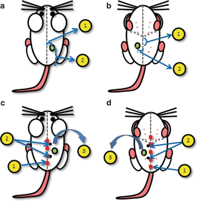
Schematics for the location of tumor implantation and surgery . (a) Schematic for tumor cell injection into the dorsal flank at a location (1) 5–10 mm lateral to midline and (2) 20–30 mm cranial to base of tail. (b) Schematic for tumor cell injection into the fourth mammary fat pad at a location (1) 10–20 mm caudal to xyphoid process of sternum and (2) 5–10 mm lateral to midline. (c) Surgical schematic for dorsal tumors: (1) midline incision from 5 mm above base of tail to near apex of shoulder, (2) location of two suture attachment points along midline incision used to stabilize the tissue, (3) separation skin flap from underlying tissue and reflection. (d) Surgical schematic for ventral tumors: (1) midline incision from 5 mm above pubic symphysis to 10 mm above xyphoid process of sternum, (2) location of two suture attachment points along midline incision used to stabilize the tissue, (3) separation skin flap from underlying tissue and reflection
-
2.
Wash and resuspend the tumor cells in cold PBS at the desired concentration (see Note 4 ). Keep the cells on ice until the injection.
-
3.
Slowly draw up 50 μL of cell suspension into an insulin syringe.
-
4.
Inject the cell suspension into the animal’s flank at the desired location (see Note 3 and Fig. 1a, b). Pinch the skin between your index finger and thumb, and gently pull it away from the mouse’s body. Inject the cell suspension slowly and evenly into the pouch created by your fingers. This should lead to a single bubble of cells beneath the skin.
-
5.
Begin measuring the tumor’s size 4 days after injection, using skin calipers. Tumors are ready for IVM when they reach 4 × 4 mm–6 × 6 mm which, depending on the tumor cell line used and the number of cells injected, is usually between 5 and 10 days post-implantation (see Note 5 ).

3.2 Setting Up the Imaging System
-
1.
Turn on the Compact Supply Unit, Metal-Halide Power Supply, confocal imaging components and computer. Open the software (see Note 6 ).
-
2.
Fix a microscope cover glass (thickness 0.12–0.19 mm) using surgical Blenderm® tape so that it overlays the imaging port located within the heating stage .
-
3.
Turn on the heated stage power supply. Set the temperature to 37 °C.
3.3 Anesthetizing the Mouse and Inserting Tail Vein Catheter (See Note 7 )
-
1.
Prepare the anesthetic solution in saline (0.9 %): a mixture of ketamine (final concentration 200 μg/g mouse) and xylazine (final concentration 10 μg/g mouse).
-
2.
Inject the anesthetic mix into the intraperitoneal (i.p.) cavity using an insulin syringe.
-
3.
After 10 min, verify the depth of anesthesia by checking the animal’s reflexes (toe-pinch withdrawal reflex—pinching with your fingertips or forceps the footpad of the mouse). The catheter insertion and surgery should not be started until the animal is deeply anesthetised and no longer demonstrates the toe-pinch withdrawal reflex.
-
4.
To assemble the venous catheter, a 1 mL syringe, polyethylene tubing (Ø 0.28 mm, length 15 cm) and two 30G × 1/2 in. needles are required. Using a hemostat , bend one of the needles back and forth until it cleanly breaks off from the hub. Insert the blunt end of the needle into one end of the catheter tubing. The needle insertion is aided by holding it with a hemostat or forceps. Fill a 1 mL slip-tip syringe with 100 U heparin in 0.9 % saline and attach the second 30G needle. Slip the tubing over the second needle and dispense the contents of the syringe to fill the tubing with heparin containing saline and remove air bubbles.
-
5.
Position the anesthetised mouse on its side so the tail vein (located laterally on the tail) is positioned facing up. Clean the tail with 70 % alcohol .
-
6.
Warm the tail using a heating lamp or warm water, to dilate the vein.
-
7.
Using your dominant hand to hold the catheter, grasp the tail between the thumb and index finger of your other hand, thumb on top, then pull back slightly so the tail is taut. Using forceps, hold the catheter needle bevel up and pierce the skin at a flat angle. Advance the needle ahead several mm into the vein.
-
8.
To verify the catheter was properly inserted and the vein was not perforated, draw back on the syringe to check for a “flash” of blood entering the catheter. If blood is observed, dispense a small amount of saline into the tail vein. The plunger will move easily and the dark colored vein will become clear if the catheter was positioned correctly .
-
9.
Secure the catheter in place with Transpore® tape .
3.4 Preparing the Tumor for Imaging
-
1.
Place the mouse onto the surgical board . Turn the surgical board so that the head of the mouse is facing away from you. Use surgical tape to fix the front and back feet (see Note 8 ). Check the mouse’s vital signs. Administer anesthetic as needed to ensure the maintenance of an appropriate level of sedation.
-
2.
Disinfect the surgical area by cleaning with gauze soaked in 70 % alcohol . Dip a cotton tip swap into mineral oil and apply oil onto the surgical area to coat the animal’s fur. This will help prevent hair from contaminating the surgical incision.
-
3.
Make an initial incision through the skin:
-
4.
Using forceps and scissors carefully separate the skin and tumor from the underlying tissues. Ensure this “skin flap” remains attached, laterally, to maintain blood supply (see Note 9 ).
-
5.
Fix the tissue stabilization pedestal (35 mm petri dish or customer-built Plexiglas platform) with Transpore® tape alongside of the mouse at the position of the tumor.
-
6.
Extend the skin flap with the tumor over the tissue stabilization pedestal and secure it along the edge using 5.0 sutures with a needle holder and tape (Fig. 2).
Fig. 2 
Tumor preparation for imaging. Arrow indicates dorsal tumor implants (a, c), and ventral tumor implants (b, d). Reflected skin flaps are stretched over a pedestal (an overturned 35 mm petri dish ) and secured using the attached sutures . This positioning of the skin flap allows for surgical removal of connective tissue overlaying the tumor. Once the tumor area has been prepared, the sutures are released (not removed) and the animal is transferred to the microscope stage
-
7.
Carefully remove the connective tissue overlaying the tumor without disrupting or damaging the vasculature. To do this, gently loosen the tension placed on the sutures stretching and securing the skin, lift the connective tissue immediately adjacent to the tumor with forceps , and carefully dissect out the membrane-like connective tissue with scissors. Ensure that no vessels are damaged or cut during this process. (see Notes 10 and 11 ).
-
8.
Check tumor vasculature for bleeding and cauterize vessels as needed. Rinse the tumor with 0.9 % saline and remove excess saline with Kimwipes® tissues .
-
9.
Remove the tape securing the animal to the surgical board and transfer the mouse to the microscope stage.
-
(a)
For dorsal tumors, place the mouse on its back with the skin flap reflected out sideways so that the subcutaneous surface of the tumor is in contact with the microscope stage (Fig. 3a, c).
Fig. 3 
Tumor positioning on the microscope stage for imaging. Dorsal (a) and ventral (b) tumor preparation, top view. Dorsal (c) and ventral (d) tumor preparation, viewed from underneath the microscope stage to illustrate the positioning of the skin flap, arrow indicates tumor. Once the animal is placed on the stage, the skin flap is extended and secured/stabilized using the attached sutures. A glass microscope slide is placed over the outside of skin flap to slightly flatten the tissue and to further stabilize the preparation
-
(b)
For ventral tumors, place the mouse on its abdomen with the skin flap reflected out sideways so that the subcutaneous surface of the tumor is in contact with the microscope stage (Fig. 3b, d).
-
(a)
-
10.
Take a glass microscope slide and position it over the skin flap so that it overlays the outside of the skin and is in direct contact with the fur. This should slightly flatten the tumor surface against the microscope stage. The slide itself should not contact the hind limbs (see Note 12 and Fig. 3). Make sure the tumor feeding vessels are adequately perfused and not restricted by the pressure of the microscope slide. This is accomplished by looking at blood flow through the microscope, which is approximated by visualizing the shadows of red blood cells and leukocyte.


3.5 Injecting Antibodies and Imaging
-
1.
Prepare a mixture of antibodies in a 1.5 mL microfuge tube using pipette and filter tips (see Notes 13 – 17 ).
-
2.
Draw back the plunger of a slip-tip 1 mL insulin syringe to get a 200 μL air space and then load antibody mix into the tip syringe using a pipette. The antibody mix will remain as a single volume of liquid held by surface tension within the tip of the syringe.
-
3.
Connect the syringe containing you antibodies to the tail vein catheter. Slowly push the plunger until the antibodies are injected into the catheter, stopping once the preloaded air space located behind the antibody mixture reaches the needle supporting the catheter. Remove the syringe used for administering the antibodies and replace it with a syringe containing heparinized 0.9 % saline. Avoid the introduction of air bubbles. Dispense 100 μL of saline to flush the antibody mix out of the catheter tubing to ensure the animal receives the full administration of labeling antibodies.
-
4.
Make sure the surgical preparation is stable. If necessary, tighten the stabilization sutures or reposition the glass slide flattening the tissue. Ensure the animal is continually anesthetised. Additional anesthesia can be injected via the catheter .
-
5.
Image the TME using the appropriate microscope settings (see Notes 2 and 14 ; Figs. 3 and 4; Supplemental Videos 1, 2, and 3).
Fig. 4 
Representative imaging of tumor microenvironment . (a) Low magnification image of vesicular stomatitis virus (VSV) infection (green) of tumor (red), Ly6G+ (cyan), F4/80+ (blue) cells, and the tumor vasculature (magenta), scale bar 200 μm. Image is a composite of 25 higher magnification images tiled and stitched. (b) 3D-reconstruction of tumor microenvironment: tumor cells (red), vessels (gray), VSV infection (green), collagen/second harmonic (cyan). Image is composed of a z-stack of ten optical sections (8 μm per section) (also suppl. Video 1). (c) IVM of lymphocyte populations within the tumor vasculature: CD4 (green), CD8 (blue) and NK cells (red), scale bar 30 μm (also suppl. Video 2). (d) IVM of CD11b (red) and Ly6G (green) stained cells within tumor vasculature, scale bar 25 μm, (also suppl. Video 3)
-
6.
Optimal imaging strategies and microscope configuration is dependent on the specific questions being addressed with IVM and the desired data to be obtained.
-
(a)
Some tumors have a high degree of background autofluorescence . In these tumors, it may be essential to select labeling fluorophores and reporter dyes that are spectrally distinct and separate from the wavelength(s) associated with the observed autofluorescence. As this phenomenon is tissue-specific, empirical determination of autofluorescence spectrums must be completed for each new tumor imaged.
-
(b)
Imaging fast moving cells/processes (such as cells within a tumor vessel) requires rapid image acquisition (high frame rate). To achieve this, platforms such as resonant scanners or spinning-disk are required. Rapid image acquisition requires extensive exposure of fluorophores to excitation lasers resulting in the potential for photo-bleaching. As such, care must be taken to select stable fluorophores (see Note 16 ).
-
(c)
Extended, time-lapsed imaging can be used to document slower processes (cell migration within the TME, cellular recruitment to a tissue following treatment). Imaging processes that occur over hours allows for much slower image acquisition rates (one frame every few minutes). This approach allows for smaller data files and protects photo-sensitive dyes, allowing for longer optimal imaging windows.
-
(d)
Visualizing deep within the TME is optimally achieved with an MP imaging platform. Several factors must be considered and controlled. Increasing laser power is required as imaging progresses deeper through a tissue. Increased laser power has the potential to cause thermal damage to the tissue resulting in cellular death and sterile inflammation . Optimal deep imaging is achieved with fluorophores that excite/emit towards the near-IR range of the spectrum as these wavelengths are less susceptible to absorption/scattering by the tissue.
-
(e)
Capturing multiple focal planes (z-stacks ) and reassembling them into a single image allows for the generation of 3D reconstructions of the TME. To ensure optimal 3D model generation, rapid image acquisition is required so that the cells within the TME do not move during capture of the focal planes. Additionally, the use of MP imaging generally results in higher resolution 3D models as this imaging modality captures thinner optical sections at each focal plane with less out-of-focus light originating from above or below the imaging plane.
-
(a)

4 Notes
-
1.
For the described experiments, we used a Leica SP8 inverted microscope (Leica Microsystems, Concord, Ontario, Canada), equipped with 405-, 488-, 552-, and 638-nm excitation lasers, 8 kHz tandem scan head, and spectral detectors (conventional PMT and hybrid HyD detectors) for superficial imaging (up to 100 μm). This platform is also equipped with a tuneable multiphoton (MP) laser (700–1040 nm) (Newport Corporation, Irvine, CA) and external PMT and HyD detectors (Leica) for imaging deeper into the tumors (up to 500 μm). Spectral detection combined with resonant scanning confocal allows for multicolor imaging of moving cells (both in simultaneous and sequential mode). This permits the study of interactions between tumor cells and different populations of host immune and non-immune cells within the TME.
-
2.
For the described experiments we used Leica Application System X Version 1.8.1.0.13370. The dye separation software is useful for 5–6 color imaging.
-
3.
For most subcutaneous tumor model systems, inject the cells directly under the skin of the right or left hind flank, 10–15 mm lateral to the midline, 20–30 mm superior to the base of the animal’s tail (Fig. 1a). For orthotopic models of breast cancer, inject the cells into the right or left mammary fat pad, 5–10 mm lateral to the midline, 20–30 mm caudal to xyphoid process (Fig. 1b). This specific location is crucial for optimal surgical access and intravital imaging.
-
4.
Tumor cell concentration depends on the aggressiveness of the cell line and the rate of tumor growth. To get palpable tumors within 5 days, we use 2 × 10⁶ cells/mL for 4T1 and EMT6 and 2 × 10⁷ cells/mL for B16 and CT26 cell lines .
-
5.
Many tumors are not sufficiently vascularized for high-quality IVM before 4–5 days post-implantation. After 10 days post-implantation, the thick capsule established by many tumors impedes clear visualization of the TME .
-
6.
For MP imaging, specific equipment start-up procedures must be followed to ensure optimal performance. The Electro-Optical Modulator must be switched on first as it requires at least 15 min to “warm up” before achieving full modulation depth. The super-HyD detector’s power and cooling unit should be turned on before the Compact Supply Unit to protect the circuitry.
-
7.
A jugular vein catheter can be substituted for tail vein cannulation.
-
8.
Place the mouse onto its dorsum for imaging tumors growing in mammary fat pad or onto its abdomen for imaging tumors growing on the back.
-
9.
A stable surgical preparation depends upon a clean separation of tumor from the muscles and other underlying tissues. For best results:
-
(a)
The tumors should be smaller than ~6 × 6 mm, as larger tumors are more likely to grow into deeper tissues, which makes the tumor preparation more difficult;
-
(b)
The tumor cells should be injected at the specific anatomical sites outlined in Fig 1a, b, to allow for ease of surgical access.
-
(a)
-
10.
Dissecting away the connective tissue from the tumor is crucial for successful imaging. For best results:
-
(a)
The tumors should be smaller than ~6 × 6 mm, as larger tumors develop a thick capsule.
-
(b)
Use a dissecting microscope to visualize the overlaying connective tissue that must be removed.
-
(c)
Frequently moisten the surface with 0.9 % saline to preserve tissue health and aid in removal of connective tissue.
-
(a)
-
11.
Dissecting the connective tissue overlaying the mammary fat pads is more surgically challenging than from tumors grown on the flank, due to increased vasculature and propensity for bleeding.
-
12.
The application of a microscope slide helps to gently flatten the tumor, which increases the imageable area and allows for deeper imaging. Additionally, this approach helps stabilize the surgical preparation, reducing movement in the tissue being imaged. Optimal imaging is dependent on injecting tumor cells at specific anatomical location (see Note 7 ), as cells injected too proximal or distal to the mid-line will establish tumors that are more challenging to surgically prepare. Additionally, Transpore® tape can be used to stabilize the microscope slide, but care must be taken to ensure that tumor feeding blood vessels are not restricted by the additional pressure. Tumors should not be bigger than ~6 × 6 mm post-implantation as it is more challenging to “flatten” larger solid tumors without blocking at least some blood vessels.
-
13.
Although the antibody concentration should be adjusted individually, 5–10 μg per mouse can be used as a starting point .
-
14.
The selection of fluorophores will depend upon the microscope configuration and imaging conditions. In our system, we can use up to 6 colors on the confocal platform and four colors by MP imaging. For confocal IVM, we have found that combining BV421 (BD Biosciences), QD655 (Life Technologies) (excited by 405 laser), Alexa 488 , phycoerythrin (PE) , PerCP-Cy 5.5 (excited by 488 laser), and Alexa 647 (excited by 638-laser) provides excellent 6-color imaging. Four-color MP imaging at 980 nm-excitation wavelength can be achieved using BV421, Alexa 488, PE and QD655 together with the following filter sets; dichroic 560 nm followed by light path 1—dichroic 495 nm followed by a 460/50 nm filter for BV421 and a 525/50 nm filter for Alexa 488, and light path 2—620 nm dichroic followed by a 575/15 nm filter for PE and a 661/20 nm filter for QD 655.
-
15.
Administration of fluorophore-conjugated antibodies for in vivo labeling of cells has the potential for biological effects (blocking the function of specific proteins (i.e., adhesion molecules), cellular activation through Fc-receptors , complement activation, cellular depletion). As such, each antibody used for in vivo labeling must be fully characterized and vetted in carefully controlled experiments prior to drawing conclusions from IVM.
-
16.
Care must be taken when selecting fluorophores to ensure adequate photo-stability and limit quenching during periods of extended imaging. Some fluorophores, such as PE, are susceptible to photo-bleaching. Such fluorophores are not amendable to the repeated and extended excitation associated with long-term time-lapsed imaging. Better alternatives include the broad class of sulfonated dyes (e.g., Alexa Fluor®) or nanocrystal based dyes (e.g., Qdots®). These fluorophores demonstrate remarkable photo-stability and intense brightness making them optimal for IVM. Additionally, when multiplexing imaging, selection of dyes that are spectrally distinct and with limited emission overlap is important for efficient separation of individual fluorescent signals.
-
17.
The use of fluorescently conjugated antibodies to label cells and structures in vivo is dependent on permeability of the tissue to the labeling antibody. Poorly perfused or dense tumors, or tumors with a thick, impenetrable capsule frequently afford poor access for vascular-administered antibodies resulting in suboptimal (or complete absence of) labeling of desired targets. Some of these limitations can be overcome by using cells expressing genetically encoded fluorescent reporter proteins although this approach has its own potential limitations (changes in expression level of reporter genes following a specific treatment, lack of cell-lineage specificity) .
References
Elinav E, Nowarski R, Thaiss CA, Hu B, Jin C, Flavell RA (2013) Inflammation-induced cancer: crosstalk between tumours, immune cells and microorganisms. Nat Rev Cancer 13:759–771
Cook J, Hagemann T (2013) Tumour-associated macrophages and cancer. Curr Opin Pharmacol 13:595–601
Turley SJ, Cremasco V, Astarita JL (2015) Immunological hallmarks of stromal cells in the tumour microenvironment. Nat Rev Immunol 15:669–682
Hanahan D, Weinberg RA (2011) Hallmarks of cancer: the next generation. Cell 144:646–674
Pardoll DM (2012) The blockade of immune checkpoints in cancer immunotherapy. Nat Rev Cancer 12:252–264
Topalian SL, Weiner GJ, Pardoll DM (2011) Cancer immunotherapy comes of age. J Clin Oncol 29:4828–4836
Norden AD, Drappatz J, Wen PY (2009) Antiangiogenic therapies for high-grade glioma. Nat Rev Neurol 5:610–620
Smyth MJ, Ngiow SF, Ribas A, Teng MWL (2015) Combination cancer immunotherapies tailored to the tumour microenvironment. Nat Rev Clin Oncol 13:143–158. doi:10.1038/nrclinonc.2015.209
Moalli F, Proulx ST, Schwendener R, Detmar M, Schlapbach C, Stein JV (2015) Intravital and whole-organ imaging reveals capture of melanoma-derived antigen by lymph node subcapsular macrophages leading to widespread deposition on follicular dendritic cells. Front Immunol 6:114
Zal T, Chodaczek G (2010) Intravital imaging of anti-tumor immune response and the tumor microenvironment. Semin Immunopathol 32:305–317
Mempel TR, Bauer CA (2009) Intravital imaging of CD8+ T cell function in cancer. Clin Exp Metastasis 26:311–327
Lohela M, Werb Z (2010) Intravital imaging of stromal cell dynamics in tumors. Curr Opin Genet Dev 20:72–78
Deguine J, Breart B, Lemaître F, Di Santo JP, Bousso P (2010) Intravital imaging reveals distinct dynamics for natural killer and CD8(+) T cells during tumor regression. Immunity 33:632–644
Ellenbroek SIJ, van Rheenen J (2014) Imaging hallmarks of cancer in living mice. Nat Rev Cancer 14:406–418
Breart B, Lemaître F, Celli S, Bousso P (2008) Two-photon imaging of intratumoral CD8+ T cell cytotoxic activity during adoptive T cell therapy in mice. J Clin Invest 118:1390–1397
Phan TG, Bullen A (2010) Practical intravital two-photon microscopy for immunological research: faster, brighter, deeper. Immunol Cell Biol 88:438–444
Author information
Authors and Affiliations
Corresponding authors
Editor information
Editors and Affiliations
1 Electronic Supplementary Material
Below is the link to the electronic supplementary material.
4D multiphoton imaging of tumor microenvironment. Multiphoton intravital imaging of tumor cells (red), vessels (gray), virus infection (green), collagen/second harmonic (cyan). Image is composed of a z-stack of ten optical sections (8 μm per section) (MP4 2372 kb)
Spinning-disk imaging of lymphocyte populations within tumor vasculature. Spinning-disk confocal intravital imaging of CD4 (green), CD8 (blue) and NK cells (red) within the vasculature of a B16 tumor (MP4 761 kb)
Resonant-scanning confocal imaging of leukocytes within the tumor vasculature. Intravital imaging of cells stained for CD11b (red) and Ly6G (green) stained cells within vasculature or a CT26 tumor (MP4 3930 kb)
Rights and permissions
Copyright information
© 2016 Springer Science+Business Media New York
About this protocol
Cite this protocol
Naumenko, V., Jenne, C., Mahoney, D.J. (2016). Intravital Microscopy for Imaging the Tumor Microenvironment in Live Mice. In: Ursini-Siegel, J., Beauchemin, N. (eds) The Tumor Microenvironment. Methods in Molecular Biology, vol 1458. Humana Press, New York, NY. https://doi.org/10.1007/978-1-4939-3801-8_16
Download citation
DOI: https://doi.org/10.1007/978-1-4939-3801-8_16
Published:
Publisher Name: Humana Press, New York, NY
Print ISBN: 978-1-4939-3799-8
Online ISBN: 978-1-4939-3801-8
eBook Packages: Springer Protocols