Curved Steel–Concrete-Steel Sandwich Shell Under Blast

Abstract

The Finite Element (FE) method was employed to study the responses of curved SCS sandwich shells under blast loading, and their failure modes under close- and far-field blast loading were also obtained. The effects of rise height and rear to front plate thickness ratio on the blast responses of curved SCS sandwich shells were studied. In addition to the numerical studies, the single-degree-of-freedom (SDOF) model of the curved SCS sandwich shell subjected to uniformly distributed blast loading was developed, based on which the dimensionless Pressure-Impulse (P-I) diagram was constructed. In addition, the pressure and impulse asymptotes were also formulated as the geometric and material properties of the curved SCS sandwich shell by employing the energy balance principle. Finally, the procedures of using the dimensionless P-I diagram for conducting blast resistant design of the curved SCS sandwich shell were presented.

10.1 Introduction

The impact and blast resistant performances of flat steel–concrete-steel (SCS) sandwich panels were extensively studied (Anandavalli et al. 2012; Wang et al. 2015; Liew and Wang 2011), and they showed high performance in resisting impact and blast loading owing to the high ductility, spalling protection, buckling resistance and energy absorption. Recently, the curved SCS sandwich shell was appealing in resisting blast loading, since the curved shell normally outperformed flat shell under blast loading via developing compressive force along the shell. Therefore, the curved SCS sandwich shell has high potential application as blast resistant wall, as illustrated in Fig. 10.1. Up to date, several studies on punching resistance of the curved SCS sandwich shell under concentrated load were conducted (Yan et al. 2016a, b; Huang and Liew 2015). However, minimal reported works on the curved SCS sandwich shell under blast loading were found in the open literature, and the blast resistant design method of such structure was also not available.

Fig. 10.1

Curved SCS sandwich shell as blast resistant wall

The equivalent single-degree-of-freedom (SDOF) method was widely used as a simple alternative to predict the dynamic response of continuous member subjected to blast loading (Biggs 1964; Wang and Xiong 2015; Rigby et al. 2014; Morison 2006; Carta and Stochino 2013). This method was also adopted by many design guidelines (UFC 2008; ASCE 2010, 2011) to evaluate the blast-induced damage level of a structure, since it could capture the global structural response with reasonable accuracy. Another simple method to predict the damage level of a structure under blast loading is Pressure-Impulse (P–I) diagram which is an iso-damage curve for a particular structural member loaded with a particular blast load history (Mays and Smith 1995). There are mainly two methods to establish P–I diagrams, i.e., SDOF method (Li and Meng 2002a, b; Fallah and Louca 2006; Krauthammer et al. 2008; Dragos and Wu 2013) and Finite Element (FE) method (Shi et al. 2008; Mutalib and Hao 2011). As for the SDOF method, the pressure and impulse asymptotes of a P–I diagram can be directly expressed as the formulae in terms of structural parameters, such as stiffness, mass, and allowable maximum displacement, etc. Support rotation or ductility ratio was generally adopted by the design guidelines to gauge the damage level of a structure (UFC 2008; ASCE 2010, 2011), and they could be directly obtained via employing the SDOF method. Hence, support rotation or ductility ratio was normally adopted as the damage level indicator for the P–I diagram generated via employing the SDOF method. This is reasonable for the structural members like beams and slabs, but not appropriate for the column whose failure is generally governed by its residual axial strength. Therefore, the FE method with easier output of residual axial strength is preferred for establishing the P–I diagram of the column. Shi et al. (2008) and Mutalib and Hao (2011) utilized the FE method to generate the P–I diagram for reinforced concrete (RC) columns and Fiber-Reinforced Polymer (FRP) strengthened RC columns, respectively. In their studies, the residual axial strength was applied as the damage level indicator, which was more representative as compared to support rotation or ductility ratio. Parametric studies and curve-fitting might be required to establish the relationship between pressure/impulse asymptotes and structural parameters.

In this chapter, The FE method was employed to study the responses of curved SCS sandwich shells under blast loading, and their failure modes under close- and far-field blast loading were also obtained. The effects of rise height (or rise to span ratio) and rear to front plate thickness ratio on the blast responses of curved SCS sandwich shells were studied. In addition to the numerical study, the SDOF model of the curved SCS sandwich shell subjected to uniformly distributed blast loading was developed, based on which the dimensionless P–I diagram was constructed. In addition, the pressure and impulse asymptotes were also formulated as the geometric and material properties of the curved SCS sandwich shell via applying the energy balance principle.

10.2 FE Model Establishment and Verification

The explicit code in LS-DYNA was adopted in this section to simulate the dynamic responses of curved SCS sandwich shells under blast loading, and the accuracies of the established FE models were verified with the available experimental results.

10.2.1 FE Model of Curved SCS Sandwich Shell

In this study, quarter FE model of the curved SCS sandwich shell was established in Fig. 10.2 owing to the symmetry of geometry and applied blast loading. The nodes on the end plate were restricted from translation to simulate the fixed boundary condition. The steel plates were meshed using S/R Hughes-Liu shell element, and eight-node solid element with reduced integration in combination with hourglass control was employed for the concrete core (Hallquist 2006).

Fig. 10.2

copyright 2022, with permission from Elsevier

Quarter FE model of curved SCS sandwich shell, reprinted from Wang et al. (2016),

Traditional FE modeling of the SCS sandwich shell was employing solid elements for steel plates, concrete core and shear connectors (Foundoukos and Chapman 2008; Clubley et al. 2003). This detailed FE modeling approach inevitably resulted in finer meshes at shear connectors as well as steel plates adjacent to shear connectors (Foundoukos and Chapman 2008), which leaded to smaller time step and longer computing time. Anandavalli et al. (2012) employed more uniform meshing approach, i.e., using shell and link elements for the steel plates and shear connectors, respectively. In this study, a simplified approach was employed, i.e., using Hughes-Liu beam elements for shear connectors and assuming the perfect bond between concrete core and shear connectors. This approach was also used to model RC structures against blast loading, and the predictions were proven to be acceptable (Li et al. 2015; Chen et al. 2015). Figure 10.3 illustrates the modeling of the connection between steel plates and shear connectors. The circular rigid panel (with same diameter of the shear connector) is attached to the shear connector through shared node, and meanwhile tied to the steel plate. This connection modeling approach can avoid stress concentration at the steel plate caused by directly sharing the node between the shear connector and steel plate. The geometry of the curved SCS sandwich shell in this study is given in Table 10.1. Blast load was generated using keyword *LOAD_BLAST_ENHANCED (LBE) via the CONWEP feature in LS-DYNA (Hallquist 2013). The blast pressure was applied onto the front plate of the curved SCS sandwich shell and can be determined based on the amount of TNT charge, standoff distance and angle of incidence, as given below

$$P\left( t \right) = P_{r} \cos^{2} \theta + P_{i} \left( {1 + \cos^{2} \theta - 2\cos \theta } \right)$$

(10.1)

Fig. 10.3

copyright 2022, with permission from Elsevier

Simplified FE model of shear connectors, reprinted from Wang et al. (2016),

Table 10.1 Geometry of curved SCS sandwich shell (Unit: mm)

where P_r is reflected pressure, P_i is incident pressure and θ is angle of incidence.

The Continuous Surface Cap (CSC) model in LS-DYNA (Hallquist 2006) was adopted to model the behavior of concrete. This material model was developed by US Federal Highway Administration to simulate the concrete-like material subjected to high rate loading, like impact and blast (FHWA 2007a, b). The main parameters of concrete used in this analysis are given in Table 10.2. As for the simulation of steel, the Piecewise Linear Plasticity material model in LS-DYNA was employed. The material properties of steel were obtained from the tensile coupon test, and the input true stress–effective plastic strain curve is shown in Fig. 10.4. In this material model, the Cowper-Symonds model (Cowper and Symonds 1958) is used to scale the yield stress, as defined in Eq. (1.8), and the strain rate parameters C and P were 40.4 s⁻¹ and 5 for the mild steel (Jones 1988).

Table 10.2 Material properties of concrete in FE analysis

Fig. 10.4

copyright 2022, with permission from Elsevier

True stress–effective plastic strain curve for mild steel, reprinted from Wang et al. (2016),

10.2.2 FE Model Verification

There is no available experimental data on curved SCS sandwich panel subjected to blast loading in the open literature. Hence, the field blast test on the flat SCS sandwich panel (Liew and Wang 2011; Kang et al. 2013), which has similar configuration of the curved SCS sandwich shell, was adopted to validate the established FE model, and the comparisons between the FE and test results were presented in Sect. 9.2. In order to calibrate the proposed FE modeling approach of shear connectors, the static test on SCS sandwich beams with shear connectors friction-welded to the steel plates (Xie et al. 2007) was employed. The same material models, element formulations and mesh size in Sect. 10.2.1 were used herein. The geometry of the SCS beam is shown in Fig. 10.5, and the material properties are given in Table 10.3. The load–displacement response of the SCS sandwich beam under concentrated load from the test (Xie et al. 2007) is compared with the FE results with different modeling approaches of shear connectors, as shown in Fig. 10.6. All the three modeling approaches can yield similar ultimate strength. However, the discrepancy is observed at the initial loading stage, i.e., “solid elements modeling approach” by Foundoukos and Chapman (2008) shows stiffer response as compared to the test results, and “shell and link modeling approach” by Anandavalli et al. (2012) shows softer response. It is noted that the proposed “shell and beam modeling approach” shows better agreement with the test results, which validates the proposed FE modeling approach of shear connectors.

Fig. 10.5

Details of SCS sandwich beam (Unit: mm)

Table 10.3 Material properties of steel and concrete (Xie et al. 2007)

Fig. 10.6

Load–displacement response of SCS sandwich beam

10.3 Curved SCS Sandwich Shell Without Shear Connectors

The responses of the curved SCS sandwich shell without shear connectors under blast loading were first examined to obtain the dynamic response characteristics and failure modes, which will be compared with those of the curved SCS sandwich shell with shear connectors in the next section. The blast load with TNT charge weight of 20 kg and standoff distance of 0.5 m was applied to the front plate of the curved SCS shell.

Figure 10.7 shows the deformation evolution of the curved SCS sandwich shell without shear connectors, and separation between faceplates and concrete core is observed owing to the absence of shear connectors. The blast load duration is very short (about 0.5 ms), which leads to an impulsive response regime of the shell (i.e., the shell only develops negligible deformation before the blast load decaying to zero). Hence, the blast energy is first transferred to the shell as kinetic energy, and the kinetic energy will be finally dissipated by the shell as internal energy. The resistance to mass ratio of the faceplate is initially higher than that of concrete core and the same to acceleration, which results in the front plate separating from concrete core after blast pressure decaying to zero. The separation between the rear plate and concrete core is also observed with relatively large deflection, which can be attributed to the reduced resistance of the rear plate after buckling. This is also demonstrated in Fig. 10.8, i.e., the increasing rate of internal energy of the rear plate slows down when the midpoint displacement exceeds 200 mm. Figure 10.8 also shows that the concrete core dissipates the majority of blast energy. In addition, the ultimate energy absorption capacity of the concrete core is reached, as shown in Fig. 10.9. The relatively smaller blast energy dissipated by faceplates can be attributed to (1) smaller volume of faceplates as compared to concrete core, (2) early separation of the front plate and (3) buckling of the rear plate for large deflection.

Fig. 10.7

copyright 2022, with permission from Elsevier

Deformation of curved SCS sandwich shell without shear connectors under blast loading, reprinted from Wang et al. (2016),

Fig. 10.8

copyright 2022, with permission from Elsevier

Internal energy–midpoint displacement curves, reprinted from Wang et al. (2016),

Fig. 10.9

copyright 2022, with permission from Elsevier

Contours of damage parameter of concrete core, reprinted from Wang et al. (2016),

10.4 Curved SCS Sandwich Shell with Shear Connectors

The separation between faceplates and concrete core was observed for the curved SCS sandwich shell without shear connectors subjected to blast loading, which limited the blast resistant capacity of the curves SCS sandwich shell. Hence, shear connectors were introduced into the curved SCS sandwich shell to improve its blast resistant performance, and the effect of shear connectors on the blast response of the curved SCS sandwich shell was also discussed. Then, the failure modes of the curved SCS sandwich shell with shear connectors under close- and far-field blast loading were discussed. In addition, the effects of rise height (or rise to span ratio) and rear to front plate thickness ratio on the blast responses of curved SCS sandwich shells were also investigated.

10.4.1 Influence of Shear Connectors

The same blast load with 20 kg TNT charge detonated at 0.5 m away was applied to the curved SCS sandwich shell with shear connectors. Figure 10.10 presents the midpoint displacements of the front and rear plates for the two curved SCS shells. Significant reduction of displacement is observed for the curved SCS shell with shear connectors, especially for displacement of the rear plate. In addition, comparable displacement of the front and rear plate can be seen for the shell with shear connectors, which demonstrates that shear connectors can bond the faceplates to concrete core and improve blast resistance of the curved SCS sandwich shell. The amount of blast energy dissipated by the front plate, concrete core and rear plate for the two shells is presented in Fig. 10.11. The portion of blast energy dissipated by faceplates of the curved SCS shell with shear connectors is 35.5% higher than that of the shell without shear connectors. This is because shear connectors can prevent separation of faceplates from concrete core and enforce them deforming together to dissipate blast energy. In addition, higher blast energy dissipated by the rear plate as compared to the front plate is observed for both the two curved SCS shells, which is due to relatively larger deformation of the rear plate.

Fig. 10.10

copyright 2022, with permission from Elsevier

Displacement–time history of curved SCS sandwich panel, reprinted from Wang et al. (2016),

Fig. 10.11

copyright 2022, with permission from Elsevier

Comparison of internal energy of curved SCS sandwich shell with and without shear connectors, reprinted from Wang et al. (2016),

Unlike steel material, the strength of concrete under compression is much higher than that under tension, and the same to energy absorption capacity. In view of this, the curved SCS sandwich shell is superior to its flat counterpart through enforcing more portion of concrete core under compression. In CSC material model, a damage parameter, d, is employed to evaluate the damage level of concrete for single element. In this study, the average damage, d_a, defined in Eq. (10.2), is utilized to evaluate the global damage level of concrete core.

$$d_{a} = \frac{{\sum_{i = 1}^{n} {d_{i} } }}{n}$$

(10.2)

where d_i is the damage parameter of element i, and n is the total number of concrete elements. Figure 10.12 shows the internal energy versus average damage curves of concrete core for the two curved SCS shells with and without shear connectors. The two curves are found to be close when the average damage value is small. However, the concrete core of the curved SCS shell without shear connectors shows significant increase in global damage with only slight increase in internal energy, which is due to the increasing portion of concrete core under tension after separation between faceplates and concrete core. Hence, the utilization of shear connectors to increase the energy absorption capacity of concrete core is demonstrated.

Fig. 10.12

copyright 2022, with permission from Elsevier

Internal energy–average damage curves of concrete core, reprinted from Wang et al. (2016),

10.4.2 Influence of Blast Loading

In order to obtain the failure modes of curved SCS sandwich shell with shear connectors under blast loading, the blast detonations with TNT charge weight of 20, 25 and 35 kg and standoff distance of 0.5 m were selected to represent close-field blast loading, and the blast detonations with TNT charge weight of 5000, 6500 and 7500 kg and standoff distance of 10 m were selected to represent far-field blast loading.

Figure 10.13a shows the failure mode of the curved SCS sandwich shell with shear connectors under close-field blast loading, and separation of the rear plate from concrete core can be observed after tearing failure of the rear plate. However, different failure mode is observed for the curved SCS sandwich shell under far-field blast loading, as shown in Fig. 10.13b, i.e., the buckling of faceplates appears at the end of the shell first, and the subsequent buckling of the front plate is observed at the mid-span. The loading duration of close-field blast loading is significantly shorter as compared to far-filed blast loading and can be considered to act in an impulsive manner, the curved SCS sandwich shell under close-field blast loading generally experiences higher acceleration, which is prone to trigger a failure mode of separation between the rear plate and concrete core. As for the curved SCS sandwich shell under far-field blast loading, whose loading duration is longer and can be considered to act in a quasi-static or dynamic manner, the shell is prone to deform as that under quasi-static loading, showing buckling failure of faceplates.

Fig. 10.13

copyright 2022, with permission from Elsevier

Failure modes of curved SCS sandwich shell with shear connectors: a close-field and b far-field blast loading, reprinted from Wang et al. (2016),

Figure 10.14 presents the internal energy (or blast energy dissipation) ratios of concrete core to faceplates, and comparable amount of blast energy dissipated by concrete core and faceplates can be observed. For the close-field blast loading with standoff distance of 0.5 m, the blast energy dissipated by faceplates shows increase with increasing TNT charge weight before failure of the shell (from 20 to 25 kg TNT charge). However, more blast energy dissipated by concrete core is observed for the shell after failure (35 kg TNT charge), which can be attributed to the reduced blast energy dissipated by the rear plate after separating from concrete core. For the far-field blast loading with standoff distance of 10 m, the percentage of blast energy dissipated by concrete core shows increase with increasing TNT charge weight. Figure 10.14 also shows that the percentage of blast energy dissipated by faceplates of the shell under close-field blast loading is lower as compared to that under far-field blast loading at the same external work level, which can be attributed to the reduced blast energy absorption capacity of the rear plate after separation. As mentioned previously, the energy absorption capacity of concrete varies with loading path (e.g., compression or tension), and the average damage, d_a, is proposed to evaluate the global damage level of concrete core. Herein, the ratio of internal energy per unit volume to average damage is used to evaluate the energy absorption efficiency of concrete core. It can be seen in Fig. 10.15 that the energy absorption efficiency of concrete core shows increase with increasing average damage. In addition, the energy absorption efficiency of concrete core for close-field blast loading case is lower as compared to far-field blast loading case at the same average damage level, which indicates that more portion of concrete core is under tension after occurrence of separation between the rear plate and concrete core.

Fig. 10.14

copyright 2022, with permission from Elsevier

Internal energy ratio of concrete to faceplates versus external work, reprinted from Wang et al. (2016),

Fig. 10.15

copyright 2022, with permission from Elsevier

Energy absorption efficiency of concrete core versus average damage, reprinted from Wang et al. (2016),

10.4.3 Influence of Rise Height

The curved SCS sandwich shells with span of 1.2 m and four different rise heights (0, 0.3, 0.45 and 0.56 m) were subjected to close- (25 kg TNT charge with standoff distance of 0.5 m) and far-field (5000 kg TNT charge with standoff distance of 10 m) blast loading, and the external work, blast energy absorption and damage of the shell were discussed and presented as followings.

The effect of rise height on the dynamic responses of curved SCS sandwich shells under blast loading are illustrated in Table 10.4. The external work done by blast loading generally exhibits decrease with increasing rise height for both close- and far-field blast loading, i.e., the external work is reduced by 49.7% and 78.3% for close- and far-field blast loading, respectively, by increasing rise height from 0 m to 0.56 m. Since the external work done by blast loading will be dissipated by the shell as internal energy, the decrease in external work with increasing rise height also leads to the decrease in damage of concrete core and faceplates, as shown in Table 10.4. Herein, the average damage, d_a, defined in Eq. (10.2) is used to evaluate the global damage of concrete core, and the average effective plastic strain, ε_ap, defined in Eq. (10.3) (Wang and Liew 2015) is used to evaluate the global damage of faceplates.

$$\varepsilon_{ap} = \frac{{\sum_{i = 1}^{n} {\varepsilon_{pi} } }}{n}$$

(10.3)

Table 10.4 Summaries of FE results with varied rise heights

where $\varepsilon_{pi}$ is the effective plastic strain of element i, and n is the total number of faceplate elements. Table 10.4 shows that both the damages of concrete core and faceplates are reduced significantly by increasing rise height from 0 to 0.45 m. However, further increasing rise height from 0.45 to 0.56 m shows little effect on the damages of concrete core and faceplates. The effect of rise height on the energy absorption efficiency of concrete core is also illustrated in Table 10.4, and the highest energy absorption efficiency of concrete core is observed for the curved SCS sandwich shell with rise height of 0.45 m.

10.4.4 Influence of Rear to Front Plate Thickness Ratio

The rear plate of the curved SCS sandwich shell experienced higher damage as compared to the front plate from previous FE simulations, and the effect of rear to front plate thickness ratio was discussed. The dynamic responses of curved SCS sandwich shells with three different combinations of rear and front plate thickness (i.e., rear/front plate thickness of 3/5, 4/4 and 5/3 mm), under close- (25 kg TNT charge with standoff distance of 0.5 m) and far-field (5000 kg TNT charge with standoff distance of 10 m) blast loading were studied, and the external work, blast energy absorption and damage of the shell were discussed.

The effect of rear to front plate thickness ratio on the dynamic responses of curved SCS sandwich shells is shown in Table 10.5. The increase in external work with increasing rear to front plate thickness ratio is observed for the shell under close-field blast loading, whereas the external work shows decrease with increasing rear to front plate thickness ratio for the shell under far-field blast loading. However, the variation in external work by increasing rear to front plate thickness ratio from 3/5 to 5/3 is not significant. Table 10.5 also shows that the damages of concrete core and faceplates generally decrease with increasing rear to front plate thickness ratio. This is because the rear plate experiences higher damage than that of front plate, and increasing rear plate thickness is more effective in improving blast resistance of the curved SCS sandwich shell. The effect of rear to front plate thickness ratio on the energy absorption efficiency of concrete core is also presented in Table 10.5, and slight increase in energy absorption efficiency is observed by increasing rear to front plate thickness ratio from 3/5 to 5/3 (i.e., 11.0% and 7.8% increase in energy absorption efficiency for close- and far-field blast loading, respectively). This demonstrates the improvement of blast resistance of the curved SCS sandwich shell by employing thicker rear plate.

Table 10.5 Summaries of FE results with varied rear to front plate thickness ratios

10.5 SDOF Model for Curved SCS Sandwich Shell

The SDOF method was adopted to obtain the blast responses of curved SCS sandwich shells, and subsequently the dimensionless P–I diagram was constructed. The curved SCS sandwich shell under uniformly distributed blast loading can be equivalent to a SDOF system, and the procedures to establish the equation of motion (EOM) are described as follows: (a) assuming a reasonable deflection shape function, which can be obtained by applying an uniformly distributed loading on the shell in a static manner (Biggs 1964); (b) establishing the relationship between strain and mid-span displacement; (c) deriving the internal energy, kinetic energy of curved SCS sandwich shell in terms of mid-span displacement and velocity, respectively, and substituting them together with the potential energy of applied blast loading into the Lagrange’s equation of motion.

10.5.1 Deflection Shape Function

For a one-way supported curved SCS sandwich shell under uniformly distributed loading shown in Fig. 10.16, it can be simplified as an arch, as the displacement in the radial direction is predominant and its value along the width direction is almost the same. Hence, the deflection shape function of the arch under uniform line load can be adopted to represent the deflection shape function of the curved SCS sandwich shell under uniformly distributed loading. As shown in Fig. 10.17 for the elastic arch under uniform line load, q, in the radial direction, the radial displacement (inwardly positive), w(θ), and tangential displacement, v(θ), are given as follows (Dym and Williams 2011):

$$w\left( \theta \right) = \frac{{qR^{4} }}{EI}\left\{ {\left[ {\left( {\frac{{1 + \overline{I}}}{2}} \right)\theta \sin \theta } \right]C_{1} - \overline{I}C_{2} + \left( {\overline{I}\cos \theta } \right)C_{3} + \overline{I}} \right\}$$

(10.4)

$$v\left( \theta \right) = \frac{{qR^{4} }}{EI}\left\{ {\left[ {\left( {1 - \overline{I}} \right)\sin \theta - \left( {1 + \overline{I}} \right)\theta \cos \theta } \right]\frac{{C_{1} }}{2} - \left( {\overline{I}\theta } \right)C_{2} + \left( {\overline{I}\sin \theta } \right)C_{3} } \right\}$$

(10.5)

Fig. 10.16

Simplification of curved shell to an arch

Fig. 10.17

Geometry of arch

where q is uniform line load, R is radius of arch, E is Young’s modulus, I is second moment of area, $\overline{I} = {{h^{2} } \mathord{\left/ {\vphantom {{h^{2} } {12R^{2} }}} \right. \kern-\nulldelimiterspace} {12R^{2} }}$ (h is thickness of arch), C₁, C₂ and C₃ are unknown constants and can be determined by applying boundary conditions. For an arch with fixed ends, the following boundary conditions are applied:

$$w\left( \alpha \right) = 0,v\left( \alpha \right) = 0,\left. {\frac{dw}{{d\theta }}} \right|_{\theta = \alpha } = 0$$

(10.6)

Then, the constants C₁, C₂ and C₃ can be determined by substituting the boundary conditions in Eq. (10.6) into Eqs. (10.4) and (10.5) as follows:

$$C_{1} = \frac{{\overline{I}\alpha }}{{\sin \alpha - \frac{{1 + \overline{I}}}{2}\alpha \left( {\frac{\alpha }{\sin \alpha } + \cos \alpha } \right)}}$$

(10.7)

$$C_{2} = \frac{\sin \alpha }{{\sin \alpha - \frac{{1 + \overline{I}}}{2}\alpha \left( {\frac{\alpha }{\sin \alpha } + \cos \alpha } \right)}}$$

(10.8)

$$C_{3} = \frac{{\frac{{1 + \overline{I}}}{2}\alpha \left( {1 + \alpha \cot \alpha } \right)}}{{\sin \alpha - \frac{{1 + \overline{I}}}{2}\alpha \left( {\frac{\alpha }{\sin \alpha } + \cos \alpha } \right)}}$$

(10.9)

The deflection shape function in the radial direction, ϕ(θ), can be determined via dividing the radial displacement, w(θ), by the mid-span displacement of the arch, w(0), i.e.,

$$\phi \left( \theta \right) = \frac{{\sin \alpha \cdot \theta \cdot \sin \theta + \left( {\sin \alpha + \alpha \cdot cos\alpha } \right) \cdot \cos \theta - \alpha - \sin \alpha \cdot \cos \alpha }}{{\left( {1 - \cos \alpha } \right)\left( {\sin \alpha - \alpha } \right)}}$$

(10.10)

It is noted in Eq. (10.10) that the radial deflection shape function varies with angle α, which is also illustrated in Fig. 10.18. In order to simplify the calculations of axial strain, internal energy, kinetic energy and potential energy in the following sections, a deflection shape function without the variable of angle α in Eq. (10.11) is proposed, considering its minimal effect on the deflection shape function induced by the variation of angle α from 10° to 90°. It was also noted by Baker et al. (1983) that the effect of deflection shape function on the structural response under blast loading was not significant if the adopted deflection shape functions were in accordance with the actual boundary condition. Hence, the simplified deflection shape function in Eq. (10.11), showing only minimal difference with the original ones, is adopted in the following calculations.

$$\phi \left( \theta \right) = \frac{1}{2}\left[ {1 + \cos \left( {\frac{\pi }{\alpha }\theta } \right)} \right]$$

(10.11)

Fig. 10.18

Deflection shape with varying angle α

10.5.2 Strain–Displacement Relationship

Establishing the relationship between strain and mid-span displacement is a primary to derive the internal energy in terms of mid-span displacement. In this study, the uniformly distributed compressive strain on the entire arch is assumed in order to provide a simple close-form solution of internal energy and arithmetic expression of dimensionless P–I diagram. In addition, the geometry requirements of arch are also presented in this section to bring down the errors induced by this assumption.

10.5.2.1 Strain Calculation

By employing the simplified deflection shape function in Eq. (10.11), the radial displacement of an arch can be expressed as:

$$w\left( \theta \right) = \frac{1}{2}\left[ {1 + \cos \left( {\frac{\pi }{\alpha }\theta } \right)} \right]w_{m}$$

(10.12)

where w_m is the mid-span displacement. According to Fig. 10.17, the developed length of arch can be determined as:

$$L_{d} = \int\limits_{{{\pi \mathord{\left/ {\vphantom {\pi 2}} \right. \kern-\nulldelimiterspace} 2} - \alpha }}^{{{\pi \mathord{\left/ {\vphantom {\pi 2}} \right. \kern-\nulldelimiterspace} 2}}} {\sqrt {r^{2} + r^{^{\prime}2} } d\beta }$$

(10.13)

where $r = R - \frac{1}{2}\left\{ {1 + \cos \left[ {\frac{\pi }{\alpha }\left( {\frac{\pi }{2} - \beta } \right)} \right]} \right\}w_{m}$ is radius of arch after deformation, and $r^{\prime} = \frac{dr}{d\beta }$. Since it is difficult to obtain the close-form solution of the developed length, L_d, from Eq. (10.13), the following approximation is adopted to obtain the developed length of arch as:

$$L_{d} \approx \int\limits_{{{\pi \mathord{\left/ {\vphantom {\pi 2}} \right. \kern-\nulldelimiterspace} 2} - \alpha }}^{{{\pi \mathord{\left/ {\vphantom {\pi 2}} \right. \kern-\nulldelimiterspace} 2}}} {\left( {\frac{{r^{^{\prime}2} }}{2R} + r} \right)d\beta } = R\alpha \left( {\frac{1}{4}B_{1}^{2} B_{2}^{2} + 1 - B_{1} } \right)$$

(10.14)

where $B_{1} = {{w_{m} } \mathord{\left/ {\vphantom {{w_{m} } {2R}}} \right. \kern-\nulldelimiterspace} {2R}}$, $B_{2} = {{\pi^{2} } \mathord{\left/ {\vphantom {{\pi^{2} } {2\alpha }}} \right. \kern-\nulldelimiterspace} {2\alpha }}$. By adopting the assumption that compressive strain is uniformly distributed, the axial strain induced by shortening of arch, ε_c, can be determined as:

$$\varepsilon_{c} = \frac{{L_{o} - L_{d} }}{{L_{o} }} = \frac{{w_{m} }}{2R} - \frac{1}{16}\left( {\frac{{w_{m} \pi }}{R\alpha }} \right)^{2} \;\left( {\text{Positive in compression}} \right)$$

(10.15)

where L_o = Rα is original length of arch.

10.5.2.2 Geometry Requirements

In reality, the axial strain induced by shortening of arch, ε_c, is not uniformly distributed. Hence, the difference between the maximum and minimum axial strain along the arch needs to be limited to an acceptable value to bring down the errors induced by this assumption. The axial stress resultant of arch can be written as (Dym and Williams 2011):

$$N\left( \theta \right) = \frac{EA}{R}\left( {\frac{dv\left( \theta \right)}{{d\theta }} - w\left( \theta \right)} \right)$$

(10.16)

where A is cross-section area of arch. Then, substituting Eqs. (10.4) and (10.5) into Eq. (10.16) leads to

$$N\left( \theta \right) = - \frac{{qR^{3} A\overline{I}}}{I}\left( {1 + C_{1} \cos \theta } \right)$$

(10.17)

Since the first term in Eq. (10.17) is only related to geometry of the arch and applied load, the axial strain, ε_c, can be written as:

$$\varepsilon_{c} \left( \theta \right) = \overline{\varepsilon }\left( {1 + C_{1} \cos \theta } \right)$$

(10.18)

where $\overline{\varepsilon }$ is a function of applied load, geometry and material properties of arch. It is noted that the axial strain varies along the arch, ranging from $\overline{\varepsilon }\left( {1 + C_{1} \cos \alpha } \right)$ at end to $\overline{\varepsilon }\left( {1 + C_{1} } \right)$ at mid-span. Hence, the induced strain error, $er_{\varepsilon }$, can be determined as:

$$er_{\varepsilon } = \left| {\frac{{\varepsilon_{\max } - \varepsilon_{\min } }}{{\varepsilon_{\min } }}} \right| = \left| {\frac{{C_{1} \left( {\cos \alpha - 1} \right)}}{{1 + C_{1} }}} \right|$$

(10.19)

where ε_max and ε_min are the maximum and minimum axial strain along the arch, respectively. It is noted that $er_{\varepsilon }$ is a function of α and h/R, and therefore the $er_{\varepsilon }$ in terms of α and h/R are plotted in Fig. 10.19 to facilitate the selection of acceptable geometry of the arch (i.e., the arch with suitable α and h/R satisfying the allowable strain error). Figure 10.19 shows that both increasing angle α and decreasing h/R lead to the decrease of strain error.

Fig. 10.19

Effect of α and h/R on the strain error

Since the compressive strength of concrete is much higher than tensile strength, the continuous compression of arch subjected to blast loading is preferred. Therefore, it is needed to ensure the monotonic increase of axial strain with increasing mid-span displacement before the arch reaching allowable maximum deformation, which leads to the following relationship:

$$\frac{{w_{\max } }}{R} \le 4\left( {\frac{\alpha }{\pi }} \right)^{2}$$

(10.20)

where w_max is the allowable maximum mid-span displacement of the arch.

In this calculation, only the axial strain induced by shortening of arch, ε_c, is considered, and the axial strain induced by bending, ε_b, is neglected. Similarly, a geometry limit needs to be provided to ensure the resultant axial stress of ε_c and ε_b is in compression on the entire arch. According to Fig. 10.17, the curvature of arch with thickness of h can be calculated as:

$$k_c \left( \beta \right) = \frac{{\left\vert {r^2 + 2r^{{\prime}2} - rr^{\prime} } \right\vert }}{{\left( {r^2 + r^{{\prime}2} } \right)^{3 / 2} }} = \frac{1}{R}f_1 \left( {{{w_m } / R},\alpha ,\beta } \right)$$

(10.21)

where $f_{1} \left( {{{w_{m} } \mathord{\left/ {\vphantom {{w_{m} } R}} \right. \kern-\nulldelimiterspace} R},\alpha ,\beta } \right)$ is a function with w_m/R, α and β as independent variables. Then, the axial strain induced by bending at the outmost layer of arch is

$$\varepsilon_{b} = \frac{h}{2}\Delta k_{c} = \frac{h}{2R}f_{2} \left( {{{w_{m} } \mathord{\left/ {\vphantom {{w_{m} } R}} \right. \kern-\nulldelimiterspace} R},\alpha ,\beta } \right)$$

(10.22)

It is noted that the maximum axial strain induced by bending, $\varepsilon_{b,\max }$, along the arch locates at the fixed end (i.e., β = π/2-α), and therefore $\varepsilon_{b,\max }$ can be expressed as a function with w_m/R and α as independent variables, i.e.,

$$\varepsilon_{b,\max } = \frac{h}{2}\Delta k_{c} = \frac{h}{2R}f_{3} \left( {{{w_{m} } \mathord{\left/ {\vphantom {{w_{m} } R}} \right. \kern-\nulldelimiterspace} R},\alpha } \right)$$

(10.23)

The requirement of no tensile axial strain on the arch leads to

$$\left| {\frac{{\varepsilon_{b,\max } }}{{\varepsilon_{c} }}} \right| = \frac{h}{2R}f_{4} \left( {{{w_{m} } \mathord{\left/ {\vphantom {{w_{m} } R}} \right. \kern-\nulldelimiterspace} R},\alpha } \right) \le 1$$

(10.24)

It is noted that $f_{4} \left( {{{w_{m} } \mathord{\left/ {\vphantom {{w_{m} } R}} \right. \kern-\nulldelimiterspace} R},\alpha } \right)$ shows increase with increasing w_m/R. Hence, the allowable maximum mid-span displacement, w_max, is used to replace w_m in Eq. (10.24), and this can ensure no tensile axial strain on the arch with mid-span displacement less than w_max. For the curved SCS sandwich shell studied in this chapter, the ultimate strain of concrete, ε_u, can be chosen as a failure threshold of curved SCS sandwich shell under blast loading. From Eq. (10.15), the w_m/R corresponding to ε_u can be determined as:

$$\frac{{w_{\max } }}{R} = 4\left( {\frac{\alpha }{\pi }} \right)^{2} \left[ {1 - \sqrt {1 - \left( {\frac{\pi }{\alpha }} \right)^{2} \varepsilon_{u} } } \right]$$

(10.25)

Substituting Eq. (10.25) into Eq. (10.24) and setting ε_u = 0.0035 (with concrete grade no higher than C50/60) (Eurocode 2004) leads to the allowable maximum ratio of thickness to radius, (h/R)_max, with only α as the independent variable. By utilizing curve fitting method, the expression of (h/R)_max in terms of angle α can be obtained in Eq. (10.26), and the fitted curved is shown in Fig. 10.20.

$$\frac{h}{R} \le \left( \frac{h}{R} \right)_{\max } = \left( {8.925\alpha^{2} - 324.9\alpha + 7308} \right) \times 10^{ - 5} \;\left( {\alpha\, {\text{in}}^{0} } \right)$$

(10.26)

Fig. 10.20

Relationship between (h/R)_max and angle α

10.5.3 Equation of Motion

As for the curved SCS sandwich shell with the geometry shown in Fig. 10.21 subjected to uniformly distributed blast loading, the equation of motion can be formulated in Eq. (10.27) by applying the Lagrange’s equation.

$$\frac{d}{dt}\left( {\frac{dK}{{d\dot{w}_{m} }}} \right) + \frac{{d\left( {U + V} \right)}}{{dw_{m} }} = 0$$

(10.27)

Fig. 10.21

Geometry of curved SCS sandwich shell

where K is kinetic energy, U is internal energy, V is potential energy, and w_m is mid-span displacement. The kinetic energy of the curved SCS sandwich shell can be calculated as:

$$K = \frac{1}{2}\int\limits_{0}^{\alpha } {m\left[ {\phi \left( \theta \right)\dot{w}_{m} } \right]^{2} d\theta }$$

(10.28)

where m is mass per unit radian of the curved SCS sandwich shell and given in Eq. (10.29), and $\dot{w}_{m}$ is the velocity at mid-span and can be obtained by differentiating the mid-span displacement, w_m, with respect to time, t.

$$m = \left[ {\frac{1}{2}\rho_{c} \left( {r_{out}^{2} - r_{in}^{2} } \right) + \rho_{s} \left( {t_{in} r_{inm} + t_{out} r_{outm} } \right)} \right]W_{d}$$

(10.29)

where $\rho_{c}$ and $\rho_{s}$ are densities of concrete and steel, respectively, W_d is width of curved SCS sandwich shell, and other geometric parameters can be found in Fig. 10.21.

According to the assumption on axial strain in Sect. 10.5.2, i.e., the axial strain of concrete, ε_c, is uniformly distributed on the entire concrete core, the differential of internal energy of concrete core, U_c, with respect to mid-span displacement, w_m, can be formulated as:

$$\frac{{dU_{c} }}{{dw_{m} }} = V_{c} \frac{{du_{c} }}{{d\varepsilon_{c} }}\frac{{d\varepsilon_{c} }}{{dw_{m} }}$$

(10.30)

where $V_{c} = {1 \mathord{\left/ {\vphantom {1 2}} \right. \kern-\nulldelimiterspace} 2}\left( {r_{out}^{2} - r_{in}^{2} } \right)W_{d}$ is volume of concrete core, and u_c is internal energy per unit volume of concrete core. The differential of u_c with respect to ε_c can be determined as:

$$\frac{{du_{c} }}{{d\varepsilon_{c} }} = \sigma_{c} \left( {\varepsilon_{c} } \right)$$

(10.31)

where $\sigma_{c} \left( \varepsilon \right)$ specifies the relationship between compressive stress and strain of concrete and can be expressed in Eq. (10.32) according to Eurocode 2 (2004).

$$\sigma_{c} \left( {\varepsilon_{c} } \right) = \frac{{k{{\varepsilon_{c} } \mathord{\left/ {\vphantom {{\varepsilon_{c} } {\varepsilon_{o} }}} \right. \kern-\nulldelimiterspace} {\varepsilon_{o} }} - \left( {{{\varepsilon_{c} } \mathord{\left/ {\vphantom {{\varepsilon_{c} } {\varepsilon_{o} }}} \right. \kern-\nulldelimiterspace} {\varepsilon_{o} }}} \right)^{2} }}{{1 + \left( {k - 2} \right){{\varepsilon_{c} } \mathord{\left/ {\vphantom {{\varepsilon_{c} } {\varepsilon_{o} }}} \right. \kern-\nulldelimiterspace} {\varepsilon_{o} }}}}f_{cm} \;for\;\left| \varepsilon \right| < \left| {\varepsilon_{u} } \right|$$

(10.32)

where k, f_cm, ε_o and ε_u are constants for specified concrete grade, and can be found in Eurocode 2. From Eq. (10.15), the differential of ε_c with respective to w_m can be obtained as:

$$\frac{{d\varepsilon_{c} }}{{dw_{m} }} = \frac{1}{{2R_{c} }} - \frac{{w_{m} \pi^{2} }}{{8R_{c}^{2} \alpha^{2} }}$$

(10.33)

where R_c is radius at the middle layer of concrete core, as shown in Fig. 10.21.

Similar to the calculation of dU_c/dw_m, the differential of internal energy of inner and outer steel plate with respect to mid-span displacement (dU_si/dw_m and dU_so/dw_m) can be calculated as well. Herein, the elastic–plastic-hardening constitutive model in Eq. (10.34) is employed to determine the stress–strain relationship of steel.

$$\sigma_{s} \left( {\varepsilon_{s} } \right) = \left\{ \begin{gathered} E_{s} \varepsilon_{s} \begin{array}{*{20}c} {\begin{array}{*{20}c} {} & {} & {} \\ \end{array} } & {} & {} & {\varepsilon_{s} \le \varepsilon_{y} } \\ \end{array} \hfill \\ E_{s} \varepsilon_{y} + \alpha_{E} E_{s} \left( {\varepsilon_{s} - \varepsilon_{y} } \right)\begin{array}{*{20}c} {} & {\varepsilon_{s} > \varepsilon_{y} } \\ \end{array} \hfill \\ \end{gathered} \right.$$

(10.34)

where $E_{s}$, $\varepsilon_{y}$, $\alpha_{E}$ are Young’s modulus, yield strain and hardening coefficient of steel. Hence, the differential of internal energy of the curved SCS sandwich shell with respect to mid-span displacement, dU/dw_m, can be obtained by summing the terms of concrete core, inner and outer steel plate as:

$$\frac{dU}{{dw_{m} }} = \frac{{dU_{c} }}{{dw_{m} }} + \frac{{dU_{si} }}{{dw_{m} }} + \frac{{dU_{so} }}{{dw_{m} }}$$

(10.35)

where U_c, U_si and U_so are internal energy of concrete core, inner and outer steel plate, respectively.

The potential energy of blast loading can be calculated as:

$$V = - W_{d} \int\limits_{0}^{\alpha } {P\left( t \right)r_{p} \phi \left( \theta \right)w_{m} \left( t \right)d\theta }$$

(10.36)

where P(t) is applied blast pressure–time history, and r_p is the radius at outmost layer of the outer steel plate, as shown in Fig. 10.21. Then, the equation of motion of the curved SCS sandwich shell can be obtained by substituting Eqs. (10.28), (10.35) and (10.36) into Eq. (10.27). The fourth-order Runge–Kutta time stepping procedure was employed to solve the equation of motion and obtain the maximum mid-span displacement of the curved SCS sandwich shell under blast loading.

10.6 P–I Diagram for Curved SCS Sandwich Shell

Figure 10.22 shows a typical P–I diagram, and the pressure and impulse asymptotes are two vital parameters that define the limiting values for pressure and impulse, respectively. As seen in Fig. 10.22, the response behavior of a structure subjected to blast loading can be categorized into impulsive, dynamic and quasi-static response regimes in accordance with the ratio of blast load duration to the natural period of the structure. The pressure and impulse asymptotes (quasi-static and impulsive response regimens) can be determined via employing the energy balance method, and the responses in the dynamic response regime can be obtained by employing the SDOF model presented in Sect. 10.5.

Fig. 10.22

Typical P–I diagram

10.6.1 Internal Energy–Displacement Relationship

The internal energy per unit width of concrete core can be calculated as:

$$\overline{U}_{c} \left( {w_{m} } \right) = \overline{V}_{c} u_{c}$$

(10.37)

where $\overline{V}_{c} = {1 \mathord{\left/ {\vphantom {1 2}} \right. \kern-\nulldelimiterspace} 2}\left( {r_{out}^{2} - r_{in}^{2} } \right)$ is the volume per unit width of concrete core, and u_c is the internal energy per unit volume of concrete core, which can be calculated as:

$$\begin{gathered} u_{c} \left( {\varepsilon_{c} } \right) = \int\limits_{0}^{{\varepsilon_{c} }} {\sigma_{c} d\varepsilon } \hfill \\ \begin{array}{*{20}r} \hfill {} \\ \end{array} \begin{array}{*{20}r} \hfill {} \\ \end{array} \begin{array}{*{20}r} \hfill {} \\ \end{array} \begin{array}{*{20}r} \hfill {} \\ \end{array} = \varepsilon_{o} f_{cm} \left[ {\frac{{\left( {k - 1} \right)^{2} {{\varepsilon_{c} } \mathord{\left/ {\vphantom {{\varepsilon_{c} } {\varepsilon_{o} }}} \right. \kern-\nulldelimiterspace} {\varepsilon_{o} }}}}{{\left( {k - 2} \right)^{2} }} - \frac{{\left( {{{\varepsilon_{c} } \mathord{\left/ {\vphantom {{\varepsilon_{c} } {\varepsilon_{o} }}} \right. \kern-\nulldelimiterspace} {\varepsilon_{o} }}} \right)^{2} }}{{2\left( {k - 2} \right)}} - \frac{{\left( {k - 1} \right)^{2} \ln \left( {\left( {k - 2} \right){{\varepsilon_{c} } \mathord{\left/ {\vphantom {{\varepsilon_{c} } {\varepsilon_{o} }}} \right. \kern-\nulldelimiterspace} {\varepsilon_{o} }} + 1} \right)}}{{\left( {k - 2} \right)^{3} }}} \right] \hfill \\ \end{gathered}$$

(10.38)

Then, substituting $\varepsilon_{c} = \frac{{w_{m} }}{{2R_{c} }} - \frac{{w_{m}^{2} \pi^{2} }}{{16R_{c}^{2} \alpha^{2} }}$ into Eq. (10.38) leads to the expression of internal energy per unit volume of concrete core in terms of mid-span displacement, $u_{c} \left( {w_{m} } \right)$. Similar to the calculation of internal energy per unit width of concrete core, the internal energy per unit width of inner and outer steel plate ($\overline{U}_{si} \left( {w_{m} } \right)$ and $\overline{U}_{so} \left( {w_{m} } \right)$) can be calculated as well. Herein, the relationship between internal energy per unit volume of steel plate and strain can be determined in Eq. (10.39) by employing the elastic–plastic-hardening constitutive model in Eq. (10.34).

$$u_s \left( {\varepsilon_s } \right) = \int\limits_0^{\varepsilon_s } {\sigma_s d\varepsilon^{\prime} } = \left\{ \begin{gathered} 0.5E\varepsilon_s^2 \begin{array}{*{20}c} {} & {} & {} & {\begin{array}{*{20}c} {} & {} & {} & {\begin{array}{*{20}c} {\begin{array}{*{20}c} {\begin{array}{*{20}c} {} & {} \\ \end{array} } & {} \\ \end{array} } & {\varepsilon_s \le \varepsilon_y } \\ \end{array} } \\ \end{array} } \\ \end{array} \hfill \\ 0.5\alpha_E E\varepsilon_s^2 + E\left( {1 - \alpha_E } \right)\left( {\varepsilon_y \varepsilon_s - 0.5\varepsilon_y^2 } \right)\begin{array}{*{20}c} {} & {\varepsilon_s > \varepsilon_y } \\ \end{array} \hfill \\ \end{gathered} \right.$$

(10.39)

Then, the internal energy per unit width of curved SCS sandwich shell can be obtained by summing the internal energy contributed by concrete core, inner and outer steel plate as:

$$\overline{U}\left( {w_{m} } \right) = \overline{U}_{c} \left( {w_{m} } \right) + \overline{U}_{si} \left( {w_{m} } \right) + \overline{U}_{so} \left( {w_{m} } \right)$$

(10.40)

where $\overline{U}_{c} \left( {w_{m} } \right)$, $\overline{U}_{si} \left( {w_{m} } \right)$ and $\overline{U}_{so} \left( {w_{m} } \right)$ are internal energy per unit width of concrete core, inner steel plate and outer steel plate, respectively.

10.6.2 Dimensionless Pressure and Impulse

The blast pressure profile is required when constructing the dimensionless P–I diagram. In this study, a triangular blast pressure profile with zero rise time given in Eq. (10.41) was adopted.

$$P\left( t \right) = \left\{ \begin{gathered} P_{\max } \left( {1 - {t \mathord{\left/ {\vphantom {t {t_{d} }}} \right. \kern-\nulldelimiterspace} {t_{d} }}} \right)\begin{array}{*{20}c} {} & {t < t_{d} } \\ \end{array} \hfill \\ 0\begin{array}{*{20}c} {\begin{array}{*{20}c} {} & {} \\ \end{array} } & {} & {} & {t \ge t_{d} } \\ \end{array} \hfill \\ \end{gathered} \right.$$

(10.41)

where P_max is peak pressure and t_d is loading duration.

When loading duration is much longer than the natural period of the curved SCS sandwich shell, i.e., $t_{d} > > T$, the load can be considered to act in a quasi-static manner since the structure will reach its maximum displacement long before the load has diminished. Equating the external work done per unit width by blast loading with the internal energy per unit width of the curved SCS sandwich shell leads to

$$\overline{U}\left( {w_{m} } \right) = \frac{1}{2}P_{\max } r_{p} w_{m} \alpha$$

(10.42)

Then, rewriting Eq. (10.42) gives a modified pressure asymptote as

$$\frac{{P_{\max } }}{{{{2\overline{U}\left( {w_{m} } \right)} \mathord{\left/ {\vphantom {{2\overline{U}\left( {w_{m} } \right)} {r_{p} w_{m} \alpha }}} \right. \kern-\nulldelimiterspace} {r_{p} w_{m} \alpha }}}} = 1 = \overline{P}$$

(10.43)

where $\overline{P}$ can be treated as the dimensionless pressure with the dimensionless pressure asymptote to be one.

When loading duration is much shorter than the natural period of the curved SCS sandwich shell, i.e., $t_{d} < < T$, the load can be considered to act in an impulsive manner. The blast energy initially transfers to the structure as kinetic energy and is finally absorbed by the structure as internal energy. Applying Momentum Theorem leads to

$$\frac{1}{4}P_{\max } r_{p} \alpha t_{d} = \frac{3}{8}\alpha \overline{m}\dot{w}_{m}$$

(10.44)

where $\overline{m} = {m \mathord{\left/ {\vphantom {m {W_{d} }}} \right. \kern-\nulldelimiterspace} {W_{d} }}$. The mid-span velocity of the curved SCS sandwich shell, $\dot{w}_{m}$, can be determined from Eq. (10.44), and the velocity of the curved SCS shell, $\dot{w}\left( \theta \right)$, can also be obtained by applying the deflection shape function, ϕ(θ). Then, the kinetic energy per unit width of the curved SCS sandwich shell can be obtained as:

$$\overline{E}_{k} = \frac{{\alpha r_{p}^{2} I^{2} }}{{3\overline{m}}}$$

(10.45)

where $I = 0.5P_{\max } t_{d}$ is impulse. Equating $\overline{E}_{k}$ with $\overline{U}\left( {w_{m} } \right)$ gives the follow relationship:

$$\frac{{\sqrt \alpha r_{p} I}}{{\sqrt {3\overline{m}\overline{U}\left( {w_{m} } \right)} }} = 1 = \overline{I}$$

(10.46)

where $\overline{I}$ can be treated as the dimensionless impulse with the dimensionless impulse asymptote to be one.

10.6.3 Dimensionless P–I Diagram Establishment

With the SDOF model in Sect. 10.5 to obtain the maximum mid-span displacement of the curved SCS sandwich shell under blast loading, the procedures to construct the dimensionless P–I diagram are described as follows:

• (1) Select the curved SCS sandwich shells with varying parameters, including geometry (angle α, radius, steel plate and concrete core thickness), material (steel and concrete grade) and blast loading (peak pressure and loading duration). It should be noted that the adopted geometry of the curved SCS sandwich shell must satisfy the geometry requirement specified in Sect. 10.5.

• (2) Obtain the maximum mid-span displacements of curved SCS sandwich shells with varying geometries, materials and blast loadings via employing the SDOF model and plot the pairs of dimensionless pressures, $\overline{P}$, and impulses, $\overline{I}$, in Fig. 10.23. (The dimensionless pressure and impulse are defined in Eqs. (10.43) and (10.46), respectively)

  Fig. 10.23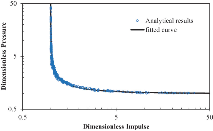

  

  Dimensionless P–I diagram from analytical model

• (3) Fit the dimensionless pressure and impulse data in Fig. 10.23 and yield the formula of dimensionless P–I diagram in Eq. (10.47).

  $$\ln \left( {\overline{P} - 1} \right) + 0.039\ln^{2} \left( {\overline{I} - 1} \right) + 0.864\ln \left( {\overline{I} - 1} \right) + 1.288 = 0$$

  (10.47)

Owing to the limitation of the established SDOF model, which cannot capture the strain rate effect, stress wave effect, confinement effect on concrete strength, etc., the FE model was adopted herein to improve the accuracy of the dimensionless P–I diagram constructed based on the SDOF method. Figure 10.24 plots the dimensionless pressures and impulses obtained from FE analyses. It is noted that the dimensionless P–I diagram constructed from SDOF method yields higher damage level as compared to that from the FE results. This is because the FE model can capture the strain rate effect, confinement effect on concrete strength, etc., and these contribute to the blast resistant improvement of the curved SCS sandwich shell. Hence, the new dimensionless P–I diagram given in Eq. (10.48) is generated by fitting the FE results to provide more accurate predictions on the damage level of the curved SCS sandwich shell under uniformly distributed blast loading.

$$\ln \left( {\overline{P} - 1.24} \right) + 0.04\ln^{2} \left( {\overline{I} - 1.38} \right) + 0.9\ln \left( {\overline{I} - 1.38} \right) - 0.1 = 0$$

(10.48)

Fig. 10.24

Modified dimensionless P–I diagram with FE analyses

10.7 Blast Resistant Design Approach

The procedures of using the dimensionless P–I diagram to perform the blast resistant design for the curved SCS sandwich shell are presented as follows:

• (1) Determine the peak pressure and loading duration for a given blast loading;

• (2) Determine the maximum mid-span displacement based on the allowable damage level;

• (3) Choose the geometric and material properties of the curved SCS sandwich shell and the geometry has to satisfy the requirement specified in Sect. 10.5.

• (4) Calculate the dimensionless pressure and impulse from Eqs. (10.43) and (10.46), respectively, with the specified geometric and material properties, maximum mid-span displacement, peak pressure and loading duration from steps (1)–(3);

• (5) Check the location of dimensionless pressure and impulse with dimensionless P–I diagram plotted in Eq. (10.47). If the data point locates below the curve, the SCS sandwich shell experiences less damage than the allowable damage level. Otherwise, the curved SCS sandwich shell exceeds the allowable damage level, and it is necessary to change the material or geometric properties of the curved SCS sandwich shell and repeat the steps (3)–(5).

Since the ductility of concrete is much lower as compared to steel and the concrete core with larger volume is the main part for resisting blast load, two damage levels of the curved SCS sandwich shell subjected to blast loading are suggested based on the compressive strain of concrete, i.e., ε_max = ε_o (damage level I) and ε_u (damage level II), where ε_o and ε_u are the strain at peak stress and ultimate strain of concrete, respectively, and their values can be found from Eurocode 2 with specified concrete grade.

In order to simplify the calculation of internal energy as well as the formula of dimensionless P–I diagram, the assumption on axial strain is employed, and the corresponding geometry requirement on the curved SCS sandwich shell for bringing down the induced error is presented in Sect. 10.5. Herein, the procedures to select the suitable geometry of the curved SCS sandwich shell are illustrated in Fig. 10.25 and described as follows:

Fig. 10.25

Flow chart for determining the geometry of the curved SCS sandwich shell

• (1) Determine the concrete core thickness, t_c, radius, R_c and anlge α.

• (2) Check the strain error allowance by utilizing Fig. 10.19 and check the ratio of thickness to radius, t_c/R_c, with the allowable value in Eq. (10.26). If any of them is not satisfied, it is needed to increase α or decrease t_c/R_c and redo the checking.

• (3) Check the geometric parameters with Eq. (10.20). If not satisfied, it is needed to increase α or R_c and redo the checking at current step.

10.8 Summary

In this chapter, the curved SCS sandwich shell was proposed to resist blast loading, and its blast response was numerically studied. In addition, a dimensionless P–I diagram of the curved SCS sandwich shell was constructed based on the SDOF model to facilitate the blast resistant design of such structure. The main findings from this chapter are summarized as follows:

• (1) The separation between faceplates and concrete core was observed for the curved SCS sandwich shell without shear connectors under close-field blast loading. With regard to the failure modes of the curved SCS sandwich shell with shear connectors, separation of the rear plate from concrete core was observed for the shell under close-field blast loading, whereas buckling of faceplates was observed for the shell under far-field blast loading.

• (2) The blast-induced deformation of the curved SCS sandwich shell with shear connectors could be significantly reduced as compared to the shell without shear connectors, which could be attributed to the improved bonding behavior between faceplates and concrete core.

• (3) The external work done by blast loading could be significantly reduced by increasing rise height. Both the damages of concrete core and faceplates could be reduced significantly by increasing rise height from 0 to 0.45 m, and further increasing rise height from 0.45 to 0.56 m showed little effect on their damages. Moreover, the highest energy absorption efficiency of concrete core was observed for the curved SCS sandwich shell with rise height of 0.45 m.

• (4) The damages of concrete core and faceplates generally showed decrease with increasing rear to front plate thickness ratio. The energy absorption efficiency of concrete core showed slight increase with increasing rear to front plate thickness ratio.

• (5) The constructed dimensionless P–I diagram using SDOF model yielded slightly higher damage as compared to the FE predictions, and therefore the FE model was employed to improve the accuracy of the dimensionless P–I diagram. In addition, the blast resistant design procedures were presented for the curved SCS sandwich shell by utilizing the dimensionless P–I diagram.

References

Anandavalli N, Lakshmanan N, Rajasankar J et al (2012) Numerical studies on blast loaded steel-concrete composite panels. JCES 1(3):102–108
ASCE (2010) Design of blast-resistant buildings in petrochemical facilities. Am Soc Civ Eng
ASCE (2011) Blast protection of buildings. ASCE/SEI 59–11. Am Soc Civ Eng
Baker WE, Cox PA, Westine PS et al (1983) Explosion and hazards and evaluation. Elsevier Scientific Publishing Compay, Amsterdam
Biggs JM (1964) Introduction to structural dynamics. McGraw-Hill, New York
Carta G, Stochino F (2013) Theoretical models to predict the flexural failure of reinforced concrete beams under blast loads. Eng Struct 49:306–315
Chen W, Hao H, Chen S (2015) Numerical analysis of prestressed reinforced concrete beam subjected to blast loading. Mater Des 65: 662–674
Clubley SK, Moy SSJ, Xiao RY (2003) Shear strength of steel-concrete-steel composite panels. Part II–detailed numerical modelling of performance. J Constr Steel Res 59:795–808
Cowper GR, Symonds PS (1958) Strain hardening and strain rate effects in the impact loading of cantilever beams. Applied Mathematics Report, Brown University
Dragos J, Wu C (2013) A new general approach to derive normalised pressure impulse curves. Int J Impact Eng 62:1–12
Dym CL, Williams HE (2011) Stress and displacement estimates for arches. J Struct Eng 137(1):49–58
Eurocode 2 (2004) Design of concrete structures – Part 1–1: General rules and rules for buildings. BS EN 1992–1–1, London
Fallah AS, Louca LA (2006) Pressure-impulse diagrams for elastic-plastic-hardening and softening single-degree-of-freedom models subjected to blast loading. Int J Impact Eng 34:823–842
Federal Highway Administration (2007a) Evaluation of LS-DYNA concrete material model 159
Federal Highway Administration (2007b) Users manual for LS-DYNA concrete material model 159
Foundoukos N, Chapman JC (2008) Finite element analysis of steel-concrete-steel sandwich beams. J Constr Steel Res 64:947–961
Hallquist JO (2006) LS-DYNA theory manual. Livermore Software Technology Corporation (LSTC). Livermore, California
Hallquist JO (2013) LS-DYNA keyword user’s manual. Livermore Software Technology Corporation (LSTC). Livermore, California
Huang Z, Liew JYR (2015) Nonlinear finite element modeling and parametric study of curved steel-concrete-steel double skin composite panels infilled with ultra-lightweight cement composite. Constr Build Mater 95:922-938
Jones N (1988) Structural impact, Cambridge University Press, Cambridge/NewYork
Kang WK, Lee SC, Liew JYR (2013) Analysis of steel-concrete composite column subject to blast. P I Civil Eng-Str B 166:15–27
Krauthammer T, Astarlioglu S, Blasko J et al (2008) Pressure-impulse diagrams for the behaviour assessment of structural components. Int J Impact Eng 35:771–783
Liew JYR, Wang TY (2011) Novel steel-concrete-steel sandwich composite plates subjected to impact and blast load. Adv Struct Eng 14(4):673–686
Li QM, Meng H (2002a) Pressure-impulse diagram for blast loads based on dimensional analysis and single-degree-of-freedom mode. J Eng Mech 1(87):87–92
Li QM, Meng H (2002b) Pulse loading shape effects on pressure-impulse diagram of an elastic-plastic, single-degree-of-freedom structural model. Int J Mech Sci 44:1985–1998
Li X, Chen JF, Lu Y et al (2015) Modelling static and dynamic FRP-concrete bond behaviour using a local concrete damage model. Adv Struct Eng 18(1):45–58
Mays G, Smith PD (1995) Blast effects on buildings: Design of buildings to optimize resistance to blast loading. T. Telford, London
Morison CM (2006) Dynamic response of walls and slabs by single-degree-of-freedom analysis-a critical review and revision. Int J Impact Eng 32:1214–1247
Mutalib AA, Hao H (2011) Development of P-I diagrams for FRP strengthened RC columns. Int J Impact Eng 38:290–304
Rigby SE, Tyas A, Bennett T (2014) Elastic-plastic response of plates subjected to cleared blast loads. Int J Impact Eng 66:37–47
Shi Y, Hao H, Li ZX (2008) Numerical derivation of pressure-impulse diagrams for prediction of RC column damage to blast loads. Int J Impact Eng 35:1213–1227
UFC 3–340–02 (2008) Structures to resist the effects of accidental explosions. US Department of Army, Navy and the Air Force, Washington, DC
Wang Y, Liew JYR (2015) Blast performance of water tank with energy absorbing support. Thin Wall Struct 96:1–10
Wang Y, Liew JYR, Lee SC (2015) Theoretical models for axially restrained steel-concrete-steel sandwich panels under blast loading. Int J Impact Eng 76:221–231
Wang Y, Xiong MX (2015) Analysis of axially restrained water storage tank under blast loading. Int J Impact Eng 86:167–178
Wang Y, Zhai X (2019) Development of dimensionless P-I diagram for curved SCS sandwich shell subjected to uniformly distributed blast pressure. Front Struct Civ Eng 13(6):1432–1445
Wang Y, Zhai X, Lee SC et al (2016) Response of curved steel-concrete-steel shells subjected to blast loading. Thin Wall Struct 108:185–192
Xie M, Foundoukos N, Chapman JC (2007) Static tests on steel-concrete-steel sandwich beams. J Constr Steel Res 63:735–750
Yan JB, Liew JYR, Zhang MH et al (2016a) Punching shear resistance of steel-concrete-steel sandwich composite shell structure. Eng Struct 117:470–485
Yan JB, Xiong MX, Qian X et al (2016b) Numerical and parametric study of curved steel-concrete-steel sandwich composite beams under concentrated loading. Mater Struct 49(10):3981–4001
Author information
Authors and Affiliations
Corresponding author
Rights and permissions
Copyright information
© 2023 The Author(s), under exclusive license to Springer Nature Singapore Pte Ltd.
About this chapter
Cite this chapter
Wang, Y. (2023). Curved Steel–Concrete-Steel Sandwich Shell Under Blast. In: Innovations in Impact and Blast Protections. Springer, Singapore. https://doi.org/10.1007/978-981-19-4375-1_10
Download citation
DOI: https://doi.org/10.1007/978-981-19-4375-1_10
Published:
Publisher Name: Springer, Singapore
Print ISBN: 978-981-19-4374-4
Online ISBN: 978-981-19-4375-1
eBook Packages: EngineeringEngineering (R0)